Article

Comparative Assessment of Five Machine Learning Algorithms for Supervised Object-Based Classification of Submerged Seagrass Beds Using High-Resolution UAS Imagery

1
Section for Coastal Ecology, National Institute of Aquatic Resources, Technical University of Denmark, 2800 Kgs. Lyngby, Denmark
2
Department of Biology, University of Southern Denmark, 5230 Odense, Denmark
*
Author to whom correspondence should be addressed.
Remote Sens. 2023, 15(14), 3600; https://doi.org/10.3390/rs15143600
Submission received: 3 June 2023 / Revised: 15 July 2023 / Accepted: 17 July 2023 / Published: 19 July 2023

Abstract

:
Knowledge about the spatial distribution of seagrasses is essential for coastal conservation efforts. Imagery obtained from unoccupied aerial systems (UAS) has the potential to provide such knowledge. Classifier choice and hyperparameter settings are, however, often based on time-consuming trial-and-error procedures. The presented study has therefore investigated the performance of five machine learning algorithms, i.e., Bayes, Decision Trees (DT), Random Trees (RT), k-Nearest Neighbor (kNN), and Support Vector Machine (SVM) when used for the object-based classification of submerged seagrasses from UAS-derived imagery. The influence of hyperparameter tuning and training sample size on the classification accuracy was tested on images obtained from different altitudes during different environmental conditions. The Bayes classifier performed well (94% OA) on images obtained during favorable environmental conditions. The DT and RT classifier performed better on low-altitude images (93% and 94% OA, respectively). The kNN classifier was outperformed on all occasions, while still producing OA between 89% and 95% in five out of eight scenarios. The SVM classifier was most sensitive to hyperparameter tuning with OAs ranging between 18% and 97%; however, it achieved the highest OAs most often. The findings of this study will help to choose the appropriate classifier and optimize related hyperparameter settings.

Graphical Abstract

1. Introduction

Seagrass beds are a key habitat in many coastal marine environments, providing a wide range of important ecosystem services such as improving water quality by growth-dependent nutrient uptake [1]; providing sediment stabilization [2]; supporting complex food webs [3]; and serving as a shelter, hatching, and nursery grounds for many species [4,5,6]. Despite being protected in many coastal waters, seagrass habitats around the world are in decline due to both natural and anthropogenic stressors [7,8,9,10]. Knowledge about the spatial distribution, habitat structure, and health status of seagrass beds is essential for the successful implementation of coastal conservation and restoration plans [11,12]. Different monitoring techniques are being used to measure these parameters, ranging from in-water methods involving diver observations, photos, and/or video recordings, to air- and space-borne remote sensing [13]. While in-water methods provide data of very high spatial resolution, they are often highly limited in spatial extent, time-consuming, and labor-intensive. Traditional air- and space-borne remote sensing techniques on the other hand have the ability to map large areas at a lower cost per unit area [14], but are, however, often lacking the spatial resolution required to solve specific monitoring tasks. In recent years, unoccupied aerial systems (UAS) have received attention due to their potential of compromising between the survey methods by performing monitoring tasks with a high spatial and temporal resolution over relatively large areas in a cost- and time-effective way [15,16,17]. The high spatial resolution of the data provided by UASs further allows for alternative methods of image analysis by, for example, adopting an object-based image analysis (OBIA) approach instead of using traditional pixel-based methods. With pixel-based methods, the basic analysis unit is limited to individual pixels, i.e., artificial square cells. OBIA on the other hand, groups neighboring pixels of similar character into meaningful objects in the image segmentation process and uses those as basic analysis units instead [18,19]. This is especially useful when working with data of high spatial resolution where a real-world object is usually depicted by multiple pixels, making it impossible for a single pixel alone to reflect the object’s characteristics [20]. By grouping pixels to image objects, not only spectral but also spatial, contextual, and texture features as well as hierarchical relationships of complex land-cover classes can be used to aid the classification process [18]. OBIA has therefore, on many occasions, proven to produce better results in the classification of high spatial resolution data than traditional pixel-based methods [18,21,22,23], including in shallow water marine habitats [24]. Although OBIA can improve the classification accuracy of remotely sensed data of high spatial resolution, the user is confronted with a number of challenges due to the many factors that influence the final classification result [25]. Therefore, OBIA requires careful consideration before implementation. First, meaningful image objects have to be created in the segmentation process. Then, the number and arrangement of required training and validation samples must be evaluated. Once the samples are collected, object features that represent the characteristics of the targeted classes in the most appropriate way are selected. These object features are then used to train a chosen classification algorithm, which allows for further fine-tuning of the classification algorithm’s hyperparameter. Finally, an appropriate accuracy assessment method must be implemented to evaluate the classification outcome. Numerous studies have focused on eliminating uncertainties regarding the segmentation process [26,27,28], sample schemes [29], feature selection [30,31], and accuracy assessments [32]. Also, the performance of different machine learning classifiers on high-resolution imagery was tested by many [33,34,35,36,37]. However, few have used UAS-derived imagery for a comparison of classifier performances [38,39,40], and even fewer have investigated the effect of the classifiers’ hyperparameter settings on classification accuracies [41,42]. Due to variations between study areas, data collection procedures, and environmental conditions during data collection, it is difficult to derive generalized conclusions regarding the optimal choice of classification algorithm and hyperparameter settings for a specific task. A certain approach may result in a high classification accuracy in one scenario while performing poorly in another [43]. While numerous studies have shown that an OBIA approach is indeed very useful for analyzing imagery of coastal vegetation, e.g., [24,44,45,46], the existing literature often lacks an explanation of the intricate steps taken in the OBIA workflow and the reasoning behind using a particular classification algorithm and related hyperparameter settings. By highlighting the importance of creating a solid foundation for image classification within the OBIA workflow, this study for the first time assesses the classification accuracy of five well-established machine learning classifiers—Bayes, Decision Trees (DT), Random Trees (RT), k-Nearest Neighbor (kNN) and Support Vector Machine (SVM)—using different hyperparameter settings on UAS-derived imagery of a submerged seagrass bed. The results will serve as a justification for specific classification parameter choices of future investigations and decrease the time spent on trial-and-error procedures. To cover different potential scenarios of seagrass monitoring tasks, images obtained from different altitudes (100 m, 30 m) during flights conducted during different environmental conditions (favorable, unfavorable) were used along with training sample sets of different sizes (250, 50). The overall objective of the study was to establish, which classifier performs best in a specific combination of environmental conditions, flight altitude, and available training sample set, while the more specific aim was to analyze, how tuning of the classifiers hyperparameter affects the classification accuracy.

2. Materials and Methods

2.1. Data Collection and Processing
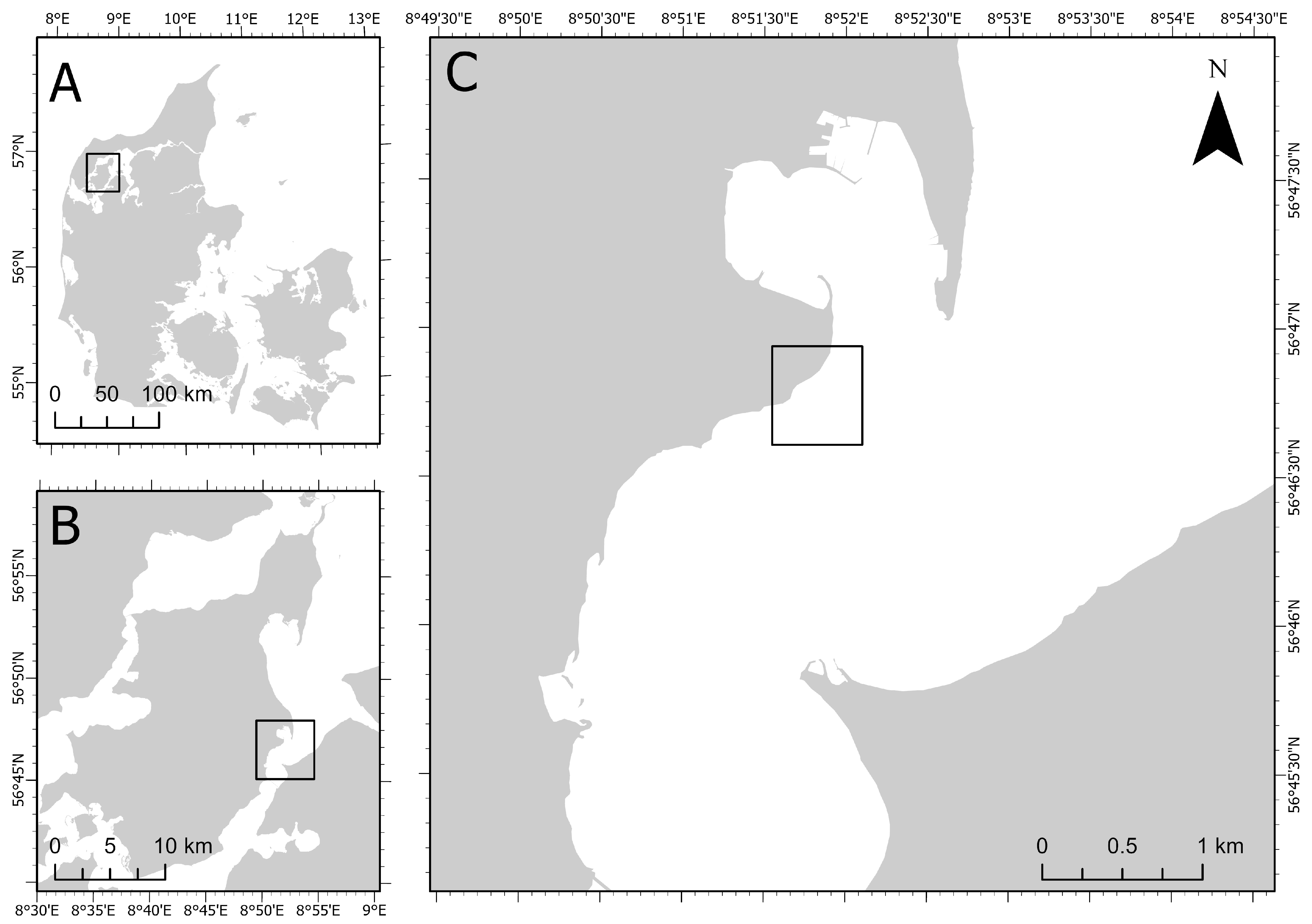
2.1.1. Study Area

The study area was situated along the eastern coast of the island Mors in the Limfjorden, Denmark (56°46′48.1″N 8°51′43.6″E) (Figure 1).
In this area, Zostera marina beds grow on a sandy bottom to a maximum depth of 2.5 m. In the past, seagrass distribution in the Limfjorden, as well as in many other Danish estuaries, has been severely affected by oxygen depletion and reduced benthic light availability caused by high nutrient loadings and resulting phytoplankton blooms [47]. Even though nutrient loadings have decreased in recent years, seagrass populations have not recovered, which explains the relatively shallow maximum growth depth of Z. marina in the study area. Other pressure factors such as waves, ice cover during winter, high water temperatures during summer, sediment perturbation by lugworms as well as anthropogenically induced destruction from fishing gear and boating result in the partial fragmentation of seagrass beds.

2.1.2. UAS Flights

The UAS platform used in this study was a consumer-grade, low-weight quadcopter of the type DJI® Phantom 4 RTK. The payload was a 20 million effective pixels 1-inch CMOS sensor-equipped RGB camera with an 84° field of view, 8.8 mm/24 mm focal length, and f. 2.8–11 aperture. In total, four flights were conducted in 2021. Two on 7 April and two on 9 September. At each date, the first flight was performed at an altitude of 100 m and the second flight at 30 m, resulting in a Ground Sample Distance (GSD) of 27.41 mm and single image dimensions of 150 × 100 m as well as 8.22 mm GSD and single image dimensions of 45 × 30 m, respectively. All images were taken with a nadir-viewing angle (90°). Image front and side overlaps were set to 75% and flight speed to 3.5 m/s during flights at 100 m altitude and 1.5 m/s during flights at 30 m altitude. One pre-programmed flight path was used for each altitude. All flights were planned and executed using the flight mission planning software UgCS® ver. 4.7.685 [48]. The flight altitudes and flight dates were chosen in order to represent four different monitoring scenarios: landscape scale studies flown at high-altitude during favorable environmental conditions (100 m_fav), landscape scale studies flown at high-altitude during less-favorable environmental conditions (100 m_unfav), small scale studies flown at low-altitude during favorable environmental conditions (30 m_fav) and small scale studies flown at low-altitude during less-favorable environmental conditions (30 m_unfav).

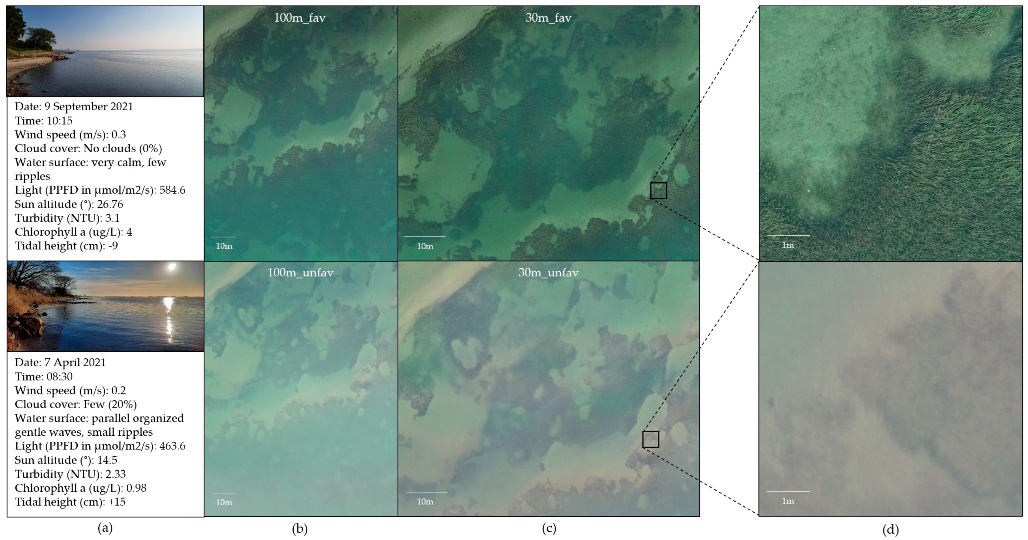
2.1.3. Environmental Conditions during UAS Flights

On both flight dates, the environmental conditions allowed visual detection of seagrass on the obtained images until the maximum depth limit. Even tough turbidity (measured with a portable turbidimeter [Hach 2100], using three samples from three locations in the study area following UAS data collection) and chlorophyll-a (measured with a spectrophotometer [photoLab 7100] using three samples from three locations in the study area following UAS data collection) concentrations were with 3.1 NTU and 4 µg/L slightly higher on 9 September (vs. 2.3 NTU and 1 µg/L on 7 April ), the overall conditions on 7 April were less favorable for UAS-based seagrass monitoring due to other factors that negatively affected the image quality, namely seagrass density, tidal height, and light conditions. Being early in the growth season, the density of seagrass was still low, resulting in a lower contrast to the surrounding sandy bottom. Contrasts were even further decreased by a tidal height of +15 cm and low light conditions with a Photosynthetic Photon Flux Density (PPFD) (measured at the shore using a handheld digital PPFD meter [Apogee Instruments MQ-500] during UAS data collection) of 319.9 µmol/m2/s. Conditions on 9 September were, on the contrary, favorable for UAS-based seagrass monitoring. A high shoot density, a tidal height of −9 cm, and a PPFD of 584.6 µmol/m2/s created a strong contrast between seagrass and sand and allowed for good visibility of details. The stronger contrast between seagrass and sand in the images obtained on 9 September is also reflected in the classes’ mean brightness values, which differed by 21.8 on the high-altitude image and 19.9 on the low-altitude image. On the images obtained on 7 April, the mean brightness values of seagrass and sand differed only by 15.7 on the high-altitude image and 12.1 on the low-altitude image. See Figure 2 for further details and visualization of the environmental conditions during the UAS flights.

2.1.4. Production of Georeferenced Orthomosaics

Both flights conducted at 100 m altitude produced 156 images each, while 415 images were obtained during the 30 m altitude flights. One georeferenced orthomosaic was created for each of the four flights by stitching the obtained images using the image processing software Agisoft Metashape Professional® ver. 1.7.4 [49]. The actual spatial resolution of the generated orthomosaics resulting from the 100 m altitude flights conducted in April and September was 2.9 cm/pixel and 3.1 cm/pixel, respectively. The orthomosaics resulting from the 30 m altitude flights conducted in April and September had a spatial resolution of 0.87 cm/pixel and 0.84 cm/pixel, respectively. For better comparability of the classification outcomes, one rectangular Region of Interest (ROI) was defined for each altitude. The ROI used for the 100 m altitude flights (ROI_1) covered 1.6 ha and resulted in dimensions of 5745 × 6241 pixels and 5171 × 5617 pixels for the images based on the flights conducted in April and September, respectively. The ROI used for the 30 m altitude flights (ROI_2) covered 1 ha and resulted in dimensions of 15,814 × 14,962 pixels and 16,489 × 15,601 pixels for the images based on the flights conducted in April and September, respectively. ROI_2 lies completely within the extent of ROI_1. The outlines of Figure 2b,c delineate the ROIs.

2.2. Object-Based Image Analysis

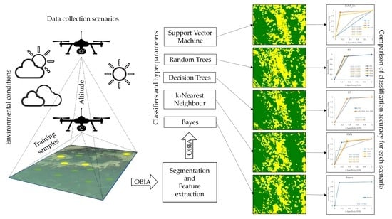
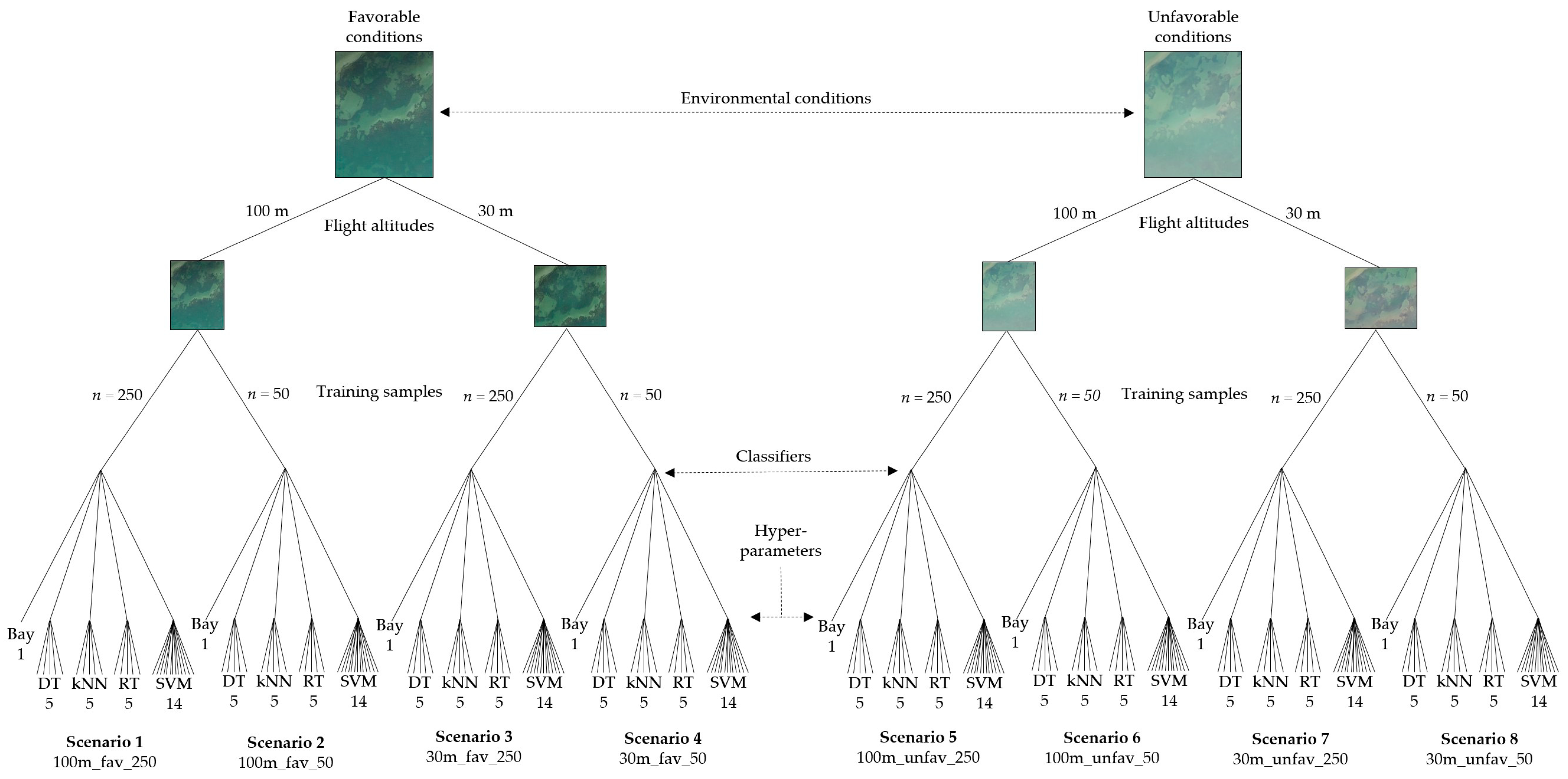
2.2.1. Experimental Setup

To assess the performance of different classification parameter settings in an OBIA approach, the results of 240 classifications were compared. These were obtained by testing five machine learning classifiers (Bayes, DT, SVM, RT, kNN) with different hyperparameter settings, using two different training sample set sizes (250, 50) and images obtained from two different altitudes (100 m, 30 m) during UAS flights conducted at different environmental conditions (favorable, unfavorable). The classification results obtained using the same values for sample set size, flight altitude, and environmental conditions were grouped into one scenario, resulting in eight scenarios. Each scenario produced 30 classification results (1 × Bayes, 5 × DT, 5 × kNN, 5 × RT, 14 × SVM). See Figure 3 for an illustration of the schematic diagram producing the 240 classification results grouped into eight scenarios.
To obtain the 240 classification results, a number of preparatory steps were taken. First, meaningful objects were created in the image segmentation process. Then, the number and arrangement of training and validation samples were defined. After sample collection, object features that represented the characteristics of the targeted classes were selected. It followed the choice of a classification algorithm with different hyperparameter settings and, finally, the classification outcomes were compared by performing an accuracy assessment.

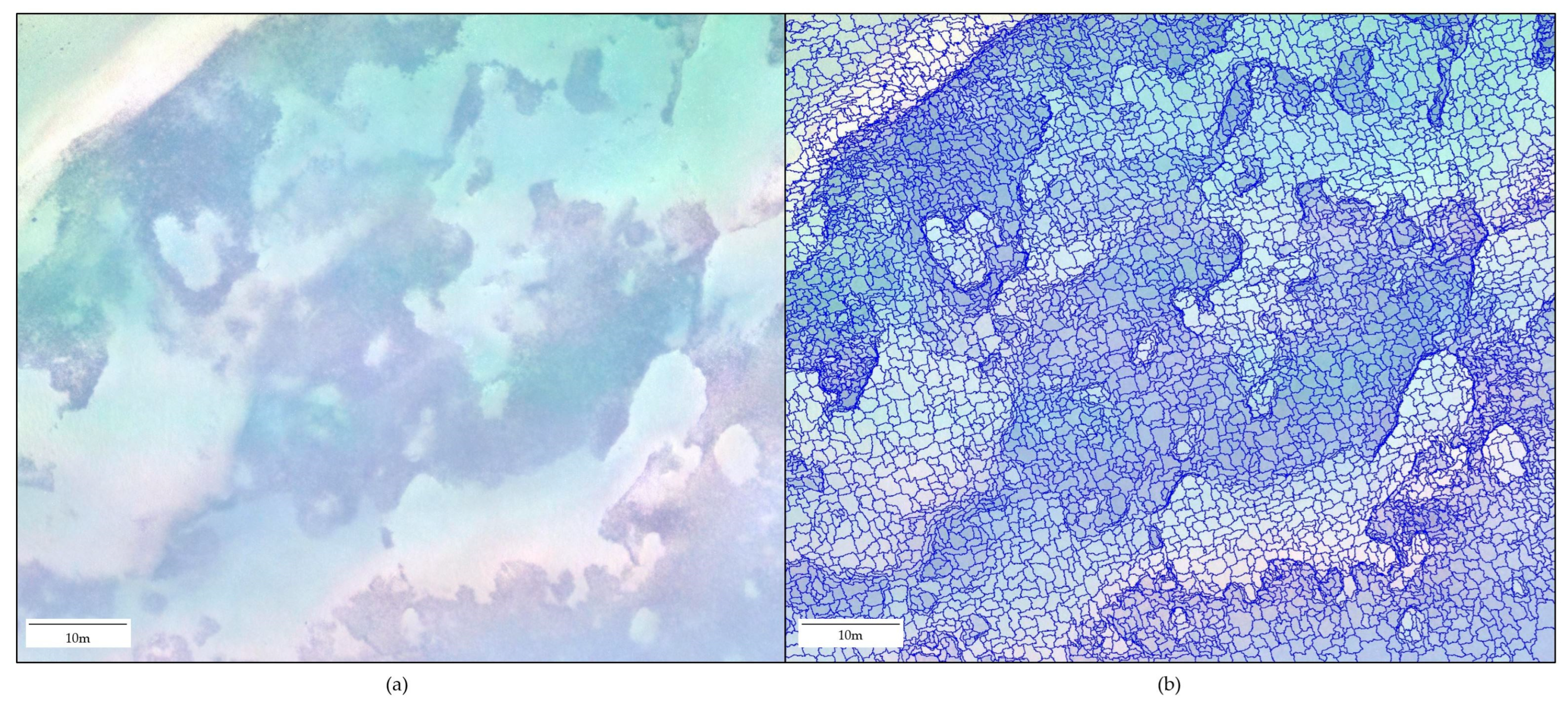
2.2.2. Image Segmentation

The first step of OBIA is the segmentation of the image into meaningful image objects by clustering pixels based on their spatial characteristics and spectral features [18]. The main goal of the segmentation is to create spatially continuous and homogeneous regions that represent the real-world objects of interest in the most appropriate way. In this study, the multiresolution segmentation algorithm in the eCognition Developer software ver. 10.1 [50] was used to create such meaningful image objects. This algorithm was introduced by Baatz and Schäpe [51] and is a widely used region-based segmentation procedure. Starting with a single pixel, the algorithm creates image objects in a bottom-up approach by pairwise clustering those neighboring objects, which results in the smallest growth of the internal spectral heterogeneity. Image objects grow until a certain heterogeneity threshold is reached, which is based on a user-defined scale parameter value. In order to set the most appropriate value for this key parameter, the Estimation-of-Scale-Parameter (ESPII) tool was used in this study, which is a fully automated, objective, and statistically based method introduced by Drǎguţ et al. [28], and further developed by Drǎguţ et al. [26]. By detecting scale shifts based on the idea of local variance of object heterogeneity within a scene, the tool calculates three optimal scales, ranging from fine scales to broader scales [28]. From these suggested scale parameter values, the one resulting in the lowest over or under-segmentation was then chosen by the authors based on a visual assessment of the segmented image objects. To obtain the scale parameter suggestions, all ESPII tool-specific parameters were set to default, except the “Use of hierarchy”, which was set to 0 (0 = No). The calculated value was then used in the multiresolution segmentation algorithm to set the scale parameter. The segmentation was performed on all three spectral bands (red, green, and blue). The shape parameter, which defines the ratio between shape characteristics and spectral features contributing to the homogeneity criterion, was set to 0.1, giving spectral features more weight. The compactness parameter, which defines the relationship between the compactness and smoothness of objects, was set to the medium value 0.5. The same approach was used to perform the image segmentation for all four images.

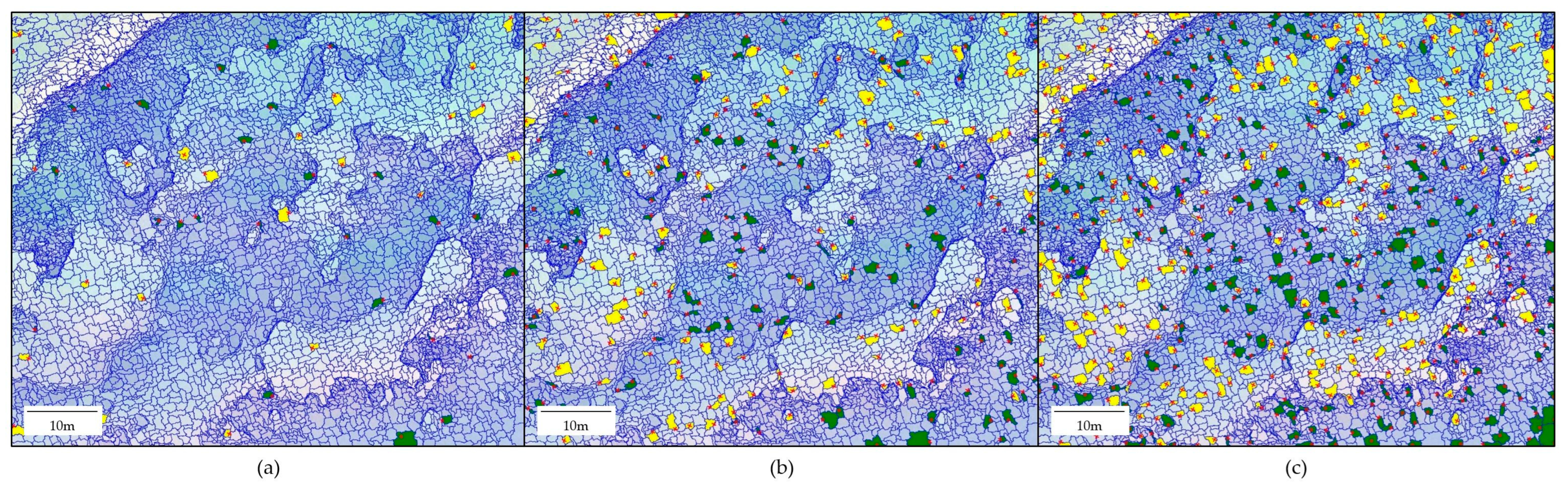
2.2.3. Training and Validation Sample Selection

Once the segmentation process was completed, subsets of the created image objects were assigned to training and validation sample sets. For the two targeted classes in this study, seagrass and sand, a “small” training sample set containing 50 samples and a “large” training sample set containing 250 samples were collected for each of the four images. The samples were distributed randomly stratified with the largest possible distance and proportionally by class using ArcGIS Pro, ver. 2.9.2. This required an a priori classification of the study area, which was performed manually based on expert knowledge and visual interpretation of the generated orthomosaic. Then, validation samples were collected, using the same method of sample distribution. The appropriate validation sample set size needed to generate an error matrix was calculated using the multinomial distribution equation originally presented by Tortora [52]
n = B Π i 1 Π i / b i 2
where n is the total sample size, B the 100th percentile of the chi-square distribution with 1 degree of freedom and 1−α/k, Π the observed class frequency, and b the desired absolute precision of the sample. The desired confidence level was set to 95% and the desired precision to 5%. The calculation was performed for all four images.

2.2.4. Feature Space

After sample collection, object features have to be selected that represent the characteristics of the targeted classes. The feature space optimization (FSO) tool within the eCognition software ver. 10.1 was used to find the optimal feature selection for this study. By evaluating the Euclidean distance in the feature space of a given training sample set, the FSO tool selects a subset of pre-selected features that results in the highest class separation distance [30]. Based on previous studies [16,39] and expert knowledge, 16 frequently used features were pre-selected in this study. These included eight textural gray level co-occurrence matrix (GLCM) features [53] (mean, homogeneity, contrast, correlation, dissimilarity, entropy, ang. 2nd moment, standard deviation) in all directions and eight spectral features (means and standard deviations of the RGB bands, maximum difference, brightness).

2.2.5. Classifiers and Hyperparameter Tuning

The performance of five well-established machine learning classifiers was tested in this study: Bayes, Decision Trees (DT), Random Trees (RT), k-Nearest Neighbor (kNN), and Support Vector Machine (SVM). All classifications were performed using the eCognition developer software ver. 10.1 on a 64-bit operating system, with Intel® Core™ i9-7900 CPU @ 3.30 GHz and 64 GB RAM.
The Bayes classifier is a readily applicable simple probabilistic classifier based on Bayes’ theorem [54] without hyperparameter tuning options. Therefore, only one classification was performed per scenario using this algorithm.
The non-parametric DT classifier [55] uses a binary recursive partitioning procedure to create classification or regression trees. In this study, the commonly used DT classification and regression tree algorithm (CART) was applied. Based on attribute value tests, the growing tree divides the training samples into homogeneous subsets until no further divisions are possible. The complexity of the tree is determined by the maximum depth parameter. The DT classifier was tested with five different maximum depth parameter values (1, 5, 10,1 5, 20). All other parameters were set to their default values (Min sample count = 0, Use surrogates = No, Max categories = 16).
The RT classifier consists of a combination of tree predictors [56]. It randomly chooses a set of features and trains each tree with a bootstrapped sample of the training data. The class label that obtains the most votes in the terminal nodes is then assigned to the training sample [57]. The RT classifier was tested using five different values for the maximum depth parameter (1, 5, 10, 15, 20). All other parameters were set to their default values (Min sample count = 0, Use surrogates = No, Max categories = 16, Active variables = 0, Max tree number = 50, Forest accuracy = 0.01, Termination criteria type = max tree numbers and forest accuracy).
The kNN classifier is a non-parametric method for classifying image objects based on the closest training examples in the feature space through an instance-based learning approach [58], where an object gets classified according to a majority vote of its k-nearest neighbors. The number of samples to be considered in the neighborhood of an object is determined by the k value. The kNN classifier was tested using five different k values (1, 5, 10, 15, 20).
The non-parametric SVM classifier [59] is a method used to find the best classification function to distinguish members of different classes in a given training sample set [60]. Based on the concept of decision planes defining decision boundaries, the algorithm then assigns image objects to specific classes. Different kernel functions can be applied in an SVM model. In this study, the SVM classifier was tested using the linear and radial basis function (rbf) kernel. An important parameter of both kernels is the cost (C) value. An additional setting of the gamma value has to be made when using the rbf kernel. The SVM classifier was tested using five different C values (2, 4, 6, 8, 10) with the linear kernel while nine different combinations of C and gamma values were tested using the rbf kernel (C = 1/g = 10−4, C = 1/g = 1, C = 1/g = 103, C = 103/g = 10−4, C = 103/g = 1, C = 103/g = 103, C = 106/g = 10−4, C = 106/g = 1, C = 106/g = 103).

2.3. Accuracy Assessment

To evaluate the performance of the different classifiers, the producer accuracy, user accuracy, and overall accuracy (OA) were calculated in a confusion error matrix [32], by using the built-in accuracy assessment tool in the eCognition Developer software ver. 10.1. The polygons created in the segmentation process served as an assessment unit, which is the most appropriate unit for the accuracy assessment of classification using an OBIA approach [32].

3. Results

3.1. Image Segmentation

The ESPII tool suggested three scale parameter levels for each image, ranging from fine to broad scale. By visual assessment of the segmented objects, the second level value was chosen for three of the four images (100 m_fav, 30 m_fav, 30 m_unfav), whereas the first level value was chosen for 100 m_unfav. The suggested scale parameter values for the 100 m altitude flights were lower than those suggested for the 30 m altitude flights (100 m_fav = 51, 30 m_fav = 101, 100 m_unfav = 61, 30 m_unfav = 91). The segmentation of 100 m_fav produced 2442 image objects while 2735 image objects were produced in the segmentation of 100 m_unfav. A total of 9667 image objects were produced in the segmentation of 30_fav and 11,738 image objects resulted from the segmentation of 30_unfav. Table 1 shows all scale parameter values calculated by the ESPII tool, with the used values highlighted. Figure 4 shows the segmentation performed on 30_unfav.

3.2. Training and Validation Sample Selection
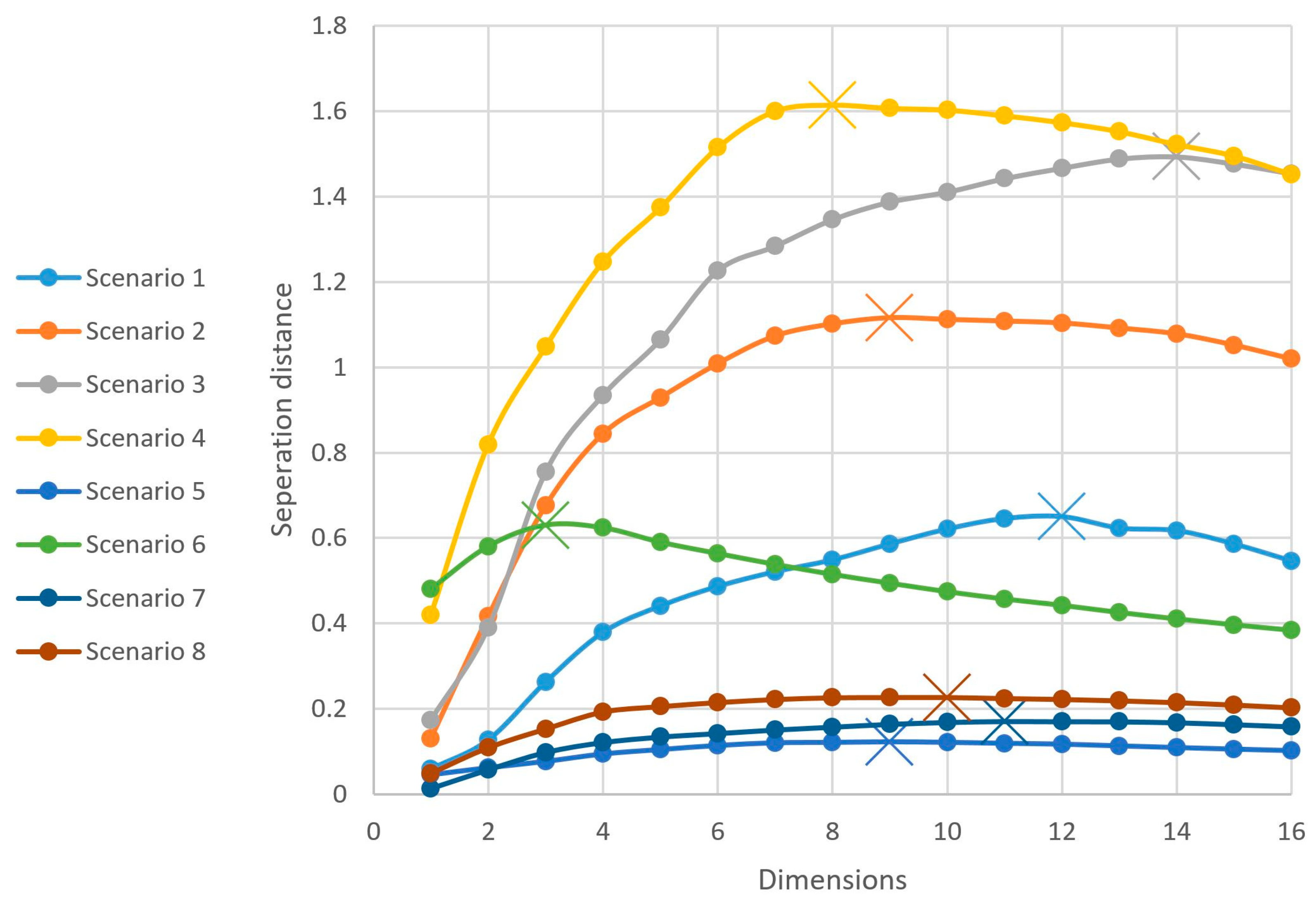
The manual classification identified 67.5% (100 m_fav) and 61.7% (100 m_unfav) seagrass cover in ROI_1 while 57.5% (30 m_fav) and 51.1% (30 m_unfav) cover were identified in ROI_2. Sample distribution and necessary training and validation sample set sizes resulting from these coverages are listed in Table 2. Figure 5 shows the distribution of training and validation samples on the 30 m_unfav image.

3.3. Feature Space

Optimal feature space dimensions calculated by the FSO too were generally larger for the same image when more samples were used. The images obtained from low-altitude flights showed larger optimal feature dimensions than the images obtained from high-altitude flights on the same date, regardless of the training sample set size, with the exception of 30 m_fav. The largest feature dimension (14) was calculated for 30 m_fav, when the sample set size was large while the smallest feature dimension (3) was calculated for 100 m_unfav, when only a few samples were available. Class separation distances were generally larger with images obtained during favorable conditions. The largest class separation distance (1.61) was calculated for 30 m_fav, when the sample set size was small, while the smallest class separation distance was calculated for 100 m_unfav (0.09), combined with a large sample set size. The GLCM Homogeneity feature was the only feature that was selected for all eight scenarios. The mean values of the red and green band, the maximum difference as well as the GLCM features Entropy and Mean were selected in all scenarios except for 100 m_unfav, combined with a small training sample set size. All other features were selected at least once, except for GLCM Correlation, which was selected in none of the scenarios. Table 3 lists the optimal feature dimensions with selected features and class distances calculated by the FSO tool. Figure 6 shows the class separation distance at a given feature dimension.

3.4. Supervised Classification

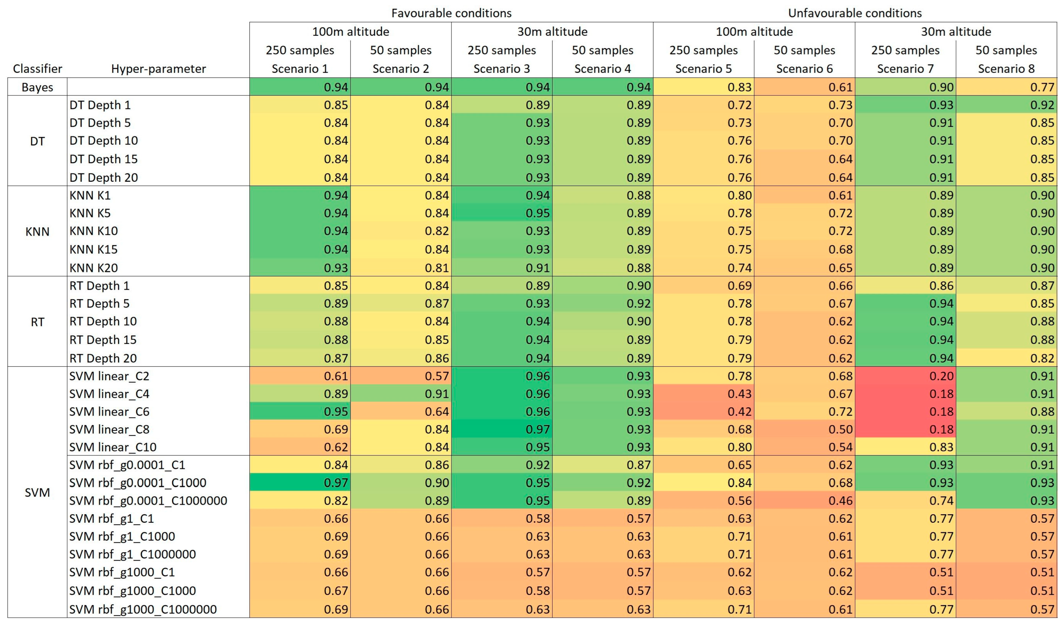
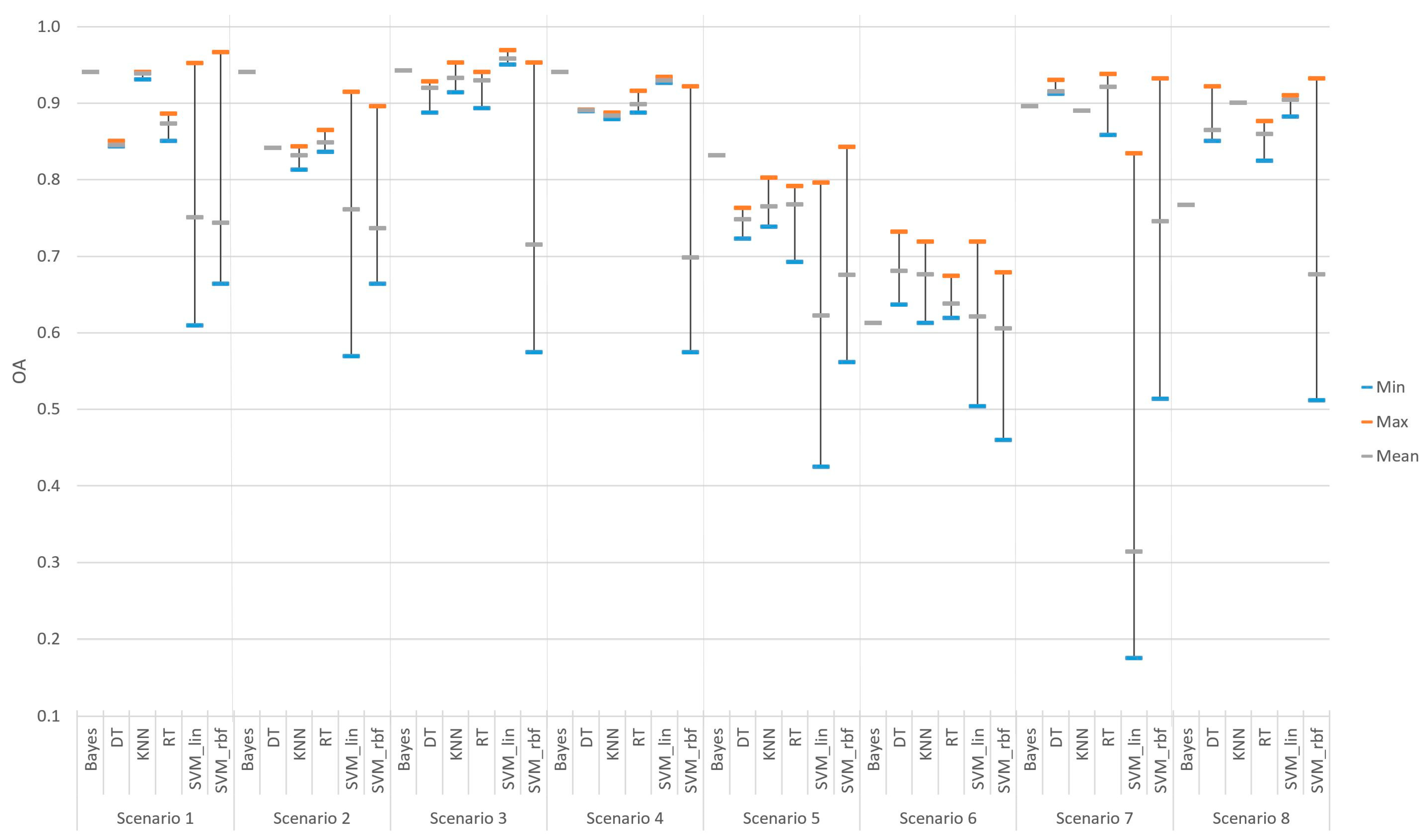
3.4.1. Classifier Performance with Optimal Hyperparameter Settings

Figure 7 lists the obtained OAs for all 240 performed classifications. Information on user and producer accuracies derived from the resulting confusion error matrices of all 240 classifications as well as receiver operating characteristic curves for each classification are presented in the Supplementary Materials. The computational time required for the single classifications varied with the size of the used training sample set, selected feature space, classifier, image resolution, and number of image objects and ranged from 53.2 s in scenario 6 with the Bayes classifier to 24 min and 10.4 s in scenario 3 with the SVM classifier. Classifiers generally performed better or equally well on images obtained at low altitudes than high altitudes. Likewise, all classifiers reached higher or equally high OAs on all images when provided with a large sample set compared to a smaller sample set, except for kNN when applied to the low-altitude image obtained during unfavorable conditions (scenario 7). Regardless of the sample size, all classifiers performed better on the high-altitude image obtained during favorable conditions (scenarios 1 and 2) than on the high-altitude image obtained during unfavorable conditions (scenarios 5 and 6). On the low-altitude image obtained during favorable conditions, all classifiers reached only better or equally high OAs as the low-altitude image obtained during unfavorable conditions when provided with a large sample set (scenario 3). When only a few samples were available, DT and kNN performed better on the low-altitude image when obtained during unfavorable conditions (scenario 8) rather than during favorable conditions (scenario 4). All images reached >85% (OA level adopted by the remote sensing community as the cutoff between acceptable and unacceptable classification results [32]). OAs with at least four classifiers, apart from the high-altitude image obtained during unfavorable conditions, reached the highest OAs at 84% with a large sample set and 73% with a small sample set (scenarios 5 and 6). The highest OA (97%) was reached by the SVM classifier on images from both altitudes obtained during favorable conditions in combination with a large sample set (scenarios 1 and 3). The lowest OA (61%) was reached by the Bayes classifier when applied to the low-altitude image obtained during unfavorable conditions in combination with a small sample set (scenario 6).
The Bayes classifier outperformed the other classifiers in two out of the eight scenarios. With an OA of 94%, Bayes was the best-performing classifier on the images from both altitudes obtained during favorable conditions when provided with a small sample set (scenarios 2 and 4). Equally high OAs were reached on the same images when provided with a large sample set (scenarios 1 and 3). When images were obtained during unfavorable conditions, the classifier only reached a good OA (90%) on the low-altitude image when provided with a large sample set (scenario 7).
The DT classifier with an OA of 73% was the best-performing classifier on the low-altitude image obtained during unfavorable conditions combined with a small sample set (scenario 6). High OAs of ≥89% were produced in all low-altitude scenarios (scenarios 3, 4, 7, and 8), while the highest OA of 93% was reached when provided with a large sample set (scenarios 3 and 7). With a small sample set, DT reached an OA of 92% on the low-altitude image obtained during unfavorable conditions (scenario 8), which is higher than the 89% OA reached on a low-altitude image obtained during favorable conditions (scenario 4). When applied to the high-altitude images, the highest OA was reached at 85% when provided with a large sample set, and the image was obtained during favorable conditions (scenario 1).
The kNN classifier was outperformed by all other classifiers in all scenarios even though high OAs of 94% and 95% were reached on images of both altitudes obtained during favorable conditions in combination with large sample sizes (scenarios 1 and 3, respectively). With 90%, the kNN classifier reached a higher OA on the low-altitude image obtained during unfavorable conditions when provided with a small sample set (scenario 8) than on the image obtained during favorable conditions (scenario 4) or with a large sample set on the same image (scenario 7), which both reached an OA of 89%.
The RT classifier was with an OA of 94% the best performing classifier on the low-altitude image obtained during unfavorable conditions when provided with a large sample set. An equally high OA was reached on the low-altitude image obtained during favorable conditions when also a large sample set was provided.
The SVM classifier outperformed the other classifiers in four out of the eight scenarios. With an OA of 97%, it was the best-performing classifier on the images from both altitudes obtained during favorable conditions when a large sample set was available (scenarios 1 and 3). On the images obtained during unfavorable conditions, it was the best-performing classifier with an OA of 84% on the high-altitude image combined with a large sample set (scenario 5) and with an OA of 93% on the low-altitude image when provided with a small sample set (scenario 8).

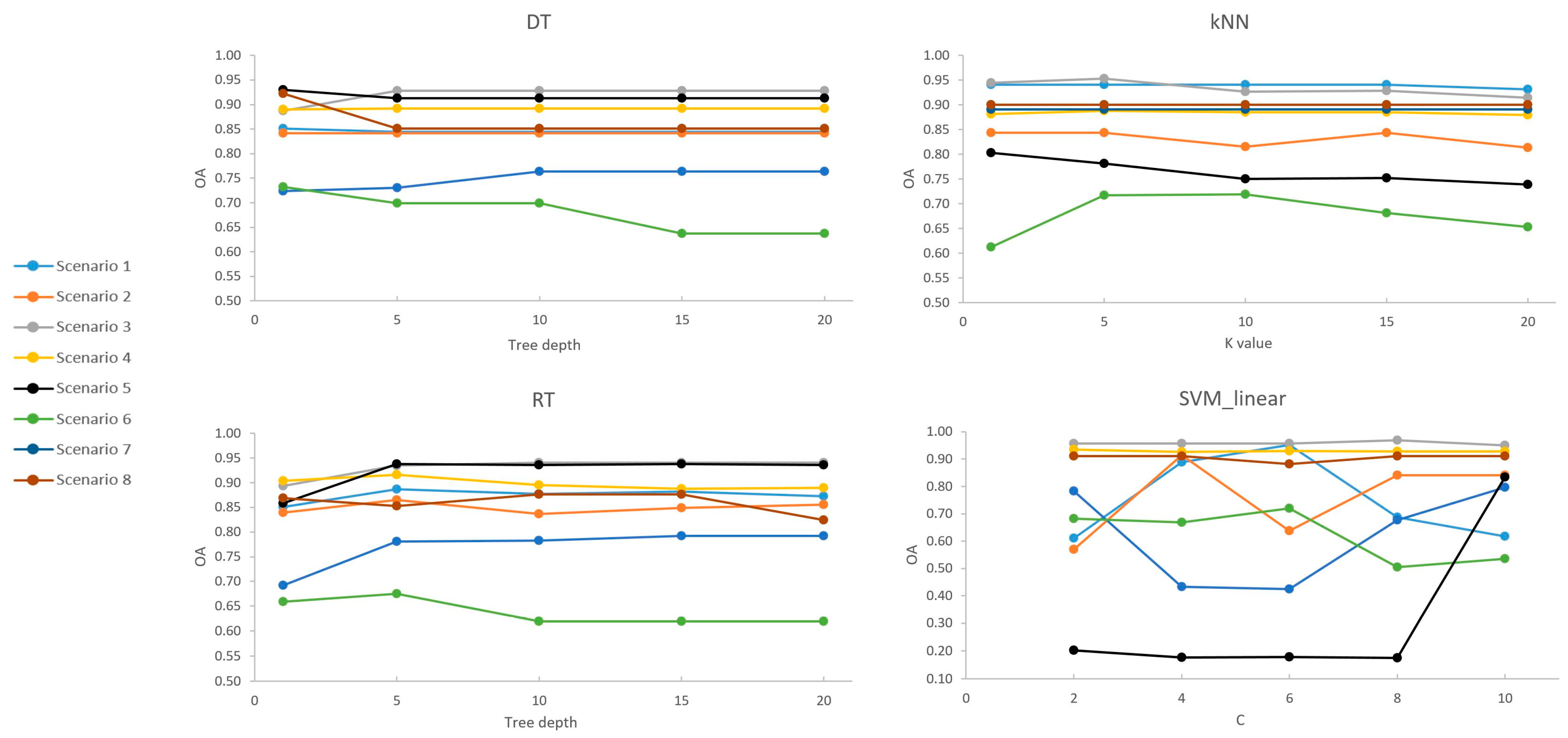
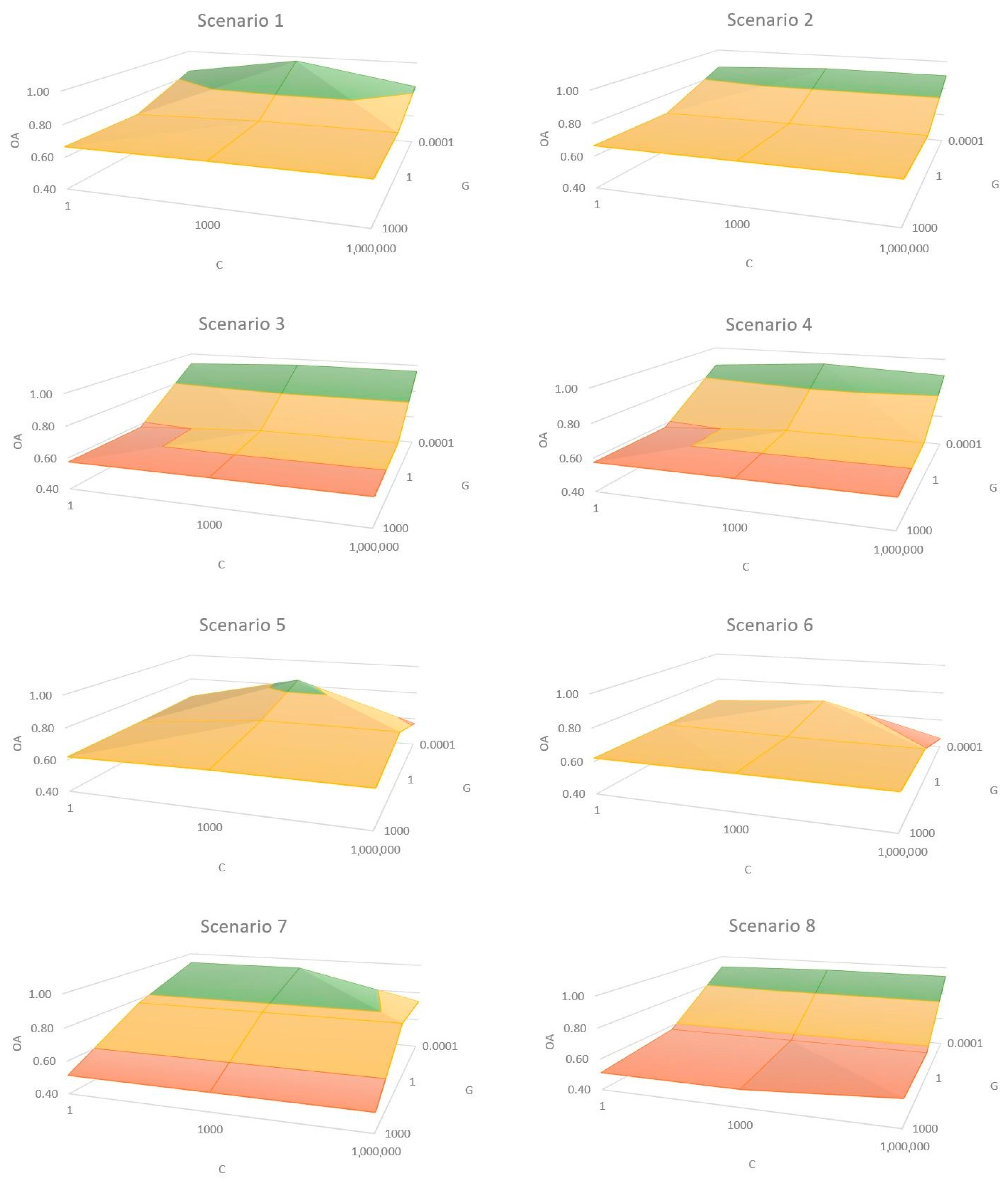
3.4.2. Sensitivity to Hyperparameter Tuning

Figure 8 illustrates variations of OAs with changing hyperparameter settings of DT, as well as those of kNN, RT, and SVM (when linear kernel used), while Figure 9 shows the ranges of produced OAs of all five classifiers per scenario, considering the produced OAs resulting from all tested hyperparameter settings.
The DT classifier was tested using five tree depth values (1, 5, 10, 15, and 20). From all classifiers, DT was the least sensitive to changes in hyperparameter settings. On the images taken from both altitudes during favorable conditions, no changes at all occurred when provided with a small sample set. In four out of the eight scenarios (scenarios 1, 3, 7, and 8), the only changes in OA were observed when changing the tree depth value from 1 to any other value. The strongest changes in OA were observed when applied to the high-altitude image obtained during unfavorable conditions combined with a small sample size (scenario 6), where the OA declined by 9% from 73% to 64% with a growing tree depth value from 1 to 20. Declines of OA with growing tree depth were also observed on the low-altitude image obtained during unfavorable conditions, regardless of sample size (scenarios 7 and 8), as well as on the high-altitude image obtained during favorable conditions combined with a large sample set. The largest improvement with growing tree depth was by 4%, observed when large sample sets were available for the low-altitude image obtained during favorable conditions as well as for the high-altitude image obtained during unfavorable conditions.
The kNN classifier was tested using five different k values (1, 5, 10, 15, & 20). No changes in OA were observed on the low-altitude image obtained during unfavorable conditions, regardless of sample size (scenarios 7 and 8). The strongest fluctuations of OA with changing k values were 6% and 11%, which occurred on the high-altitude image obtained during unfavorable conditions in combination with both a small and a large sample set, respectively (scenarios 5 and 6).
The RT classifier was tested using five tree depth values (1, 5, 10, 15, and 20). Changes of those affected OAs in all scenarios, ranging from 3% when small sample sets were used on images obtained during favorable conditions (scenarios 2 and 4) to 10% on the high-altitude image obtained during unfavorable conditions combined with a large sample set.
The SVM classifier was tested using two different kernels (linear and rbf). Tested hyperparameters in combination with the linear kernel where five different C values (2, 4, 6, 8, 10), while nine different combinations of C and gamma values were tested using the rbf kernel (C = 1/g = 10−4, C = 1/g = 1, C = 1/g = 103, C = 103/g = 10−4, C = 103/g = 1, C = 103/g = 103, C = 106/g = 10−4, C = 106/g = 1, C = 106/g = 103). The SVM classifier was the most sensitive classifier to changes in hyperparameter settings. The strongest fluctuation occurred with 75% on the low-altitude image obtained during unfavorable conditions when provided with a large sample set (scenario 7), where the OAs ranged from 18% to 93%. Lowest changes in OA were observed at 26% on the high-altitude image obtained during unfavorable conditions, where they ranged between 46% and 72% when provided with a small sample set (scenario 6). When the rbf kernel was chosen, lowering the g value increased the OAs in all scenarios and in combination with a C value set to 1000, produced the highest OAs.
Contrasting the superior performance of the SVM classifier in four out of eight scenarios with optimal hyperparameter settings, the SVM classifier also produced the lowest OAs in all scenarios, when non-optimal hyperparameter settings were chosen. Figure 10 shows the produced OAs of the SVM_rbf classifier with different C and gamma values per scenario.

4. Discussion

4.1. Object-Based Image Analysis Workflow

The presented study has investigated the performance of five well-established machine learning algorithms, i.e., Bayes, Decision Trees (DT), Random Trees (RT), k-Nearest Neighbor (kNN), and Support Vector Machine (SVM) when used for the object-based classification of submerged seagrass beds from high-resolution imagery collected by an unoccupied aerial system (UAS). A challenge of using an object-based image analysis (OBIA) approach is the flexibility of its framework, which requires careful consideration during the required preparatory steps leading to the classification. These include image segmentation and feature selection, which are often conducted in a subjective manner or based on time-consuming trial-and-error procedures, e.g., [30,39,61,62,63]. The general high overall accuracies (OAs) achieved by the tested classifiers in this study in at least some scenarios, could be an indicator of the good performance of the tools used to aid the decision on these initial but crucial steps. By applying the Estimation-of-Scale-Parameter (ESPII) tool developed by Drǎguţ et al. [26] to determine the most appropriate scale parameter for the image segmentation, this step was conducted in a statistically based, automated, repeatable, and objective way. Providing the ESPII tool with images of enhanced local contrast could further improve the performance of the tool, which could be achieved by increasing the radiometric resolution. This might prove more important than spatial resolution in the segmentation step when working with images of low spectral variance, as is often the case in the remote sensing of submerged habitats. Another adjustment of the ESPII tool to reduce over-segmentation is possible. The ESPII tool-generated scale parameter chosen in this study resulted in segments that were considerably smaller than the real-world objects. This over-segmentation was more appropriate compared to the next higher suggested scale parameter value, which resulted in under-segmentation and therefore would have required additional steps in the workflow to reclassify the under-segmented areas. Adjusting the step size parameter of the ESPII tool could be a way to obtain less over-segmentation. The feature space optimization (FSO) tool calculated the optimal feature space dimension in the feature selection step. Even though the tool is best used for feature reduction in Nearest Neighbor classifications and is known for its “black box” feature selection approach, low accuracies, and unclear feature ranking [30], it was able to reduce the number of redundant features, calculate class separation distances and therefore aid the choice of selected features. The application of other feature selection tools might have further improved this step. For example, the feature analyzing tool SEaTH (SEparability and THresholds) developed by Nussbaum et al. [31] calculates the Jeffries–Matusita distance, which is more adequate in a case of a two-class comparison, as was the case in this study. Incorporating these tools into the OBIA workflow would have a great potential of improving classification results while minimizing subjectivity and time spent on trial-and-error testing of parameters. Yet, only a few studies seem to make use of them. Hossain and Chen [27] summarized available tools and software packages for segmentation and optimization methods, while Laliberte et al. [30] evaluated feature selection tools in the context of object-based classification of high-resolution imagery.

4.2. Classifier Performance

As expected, the results of this study confirmed that the performance of the five machine learning classifiers depends on image quality and resolution, the size of the available training data set, and the algorithm-specific tuning of hyperparameter when used to classify submerged seagrass beds from UAS-derived high-resolution imagery. While in general, all classifiers were able to produce high OAs, each classifier had its strengths and weaknesses in relation to the tested scenarios. The Bayes classifier produced consistently high OAs when images were obtained during favorable conditions, even when the sample set size was small. This can be attributed to the Bayes classifier being based on conditional probability estimation. Conditional probabilities computed for objects that were created using images taken during favorable conditions provided better separation properties between classes as compared to those computed for objects that were created using images taken during unfavorable conditions, as those provided less contrast. The tree-based algorithms DT and RT performed better when applied to low-altitude images as the low-altitude images provided a better level of detail compared to the images obtained from higher altitudes. The kNN classifier was outperformed in all scenarios while still producing high OAs. Interestingly, it also performed better with fewer available training samples on the low-altitude image obtained during unfavorable conditions. This behavior, as well as the algorithm’s equally good performance on images obtained from both altitudes during favorable conditions, could be attributed to the fact that the kNN classifier does not construct an internal model in the form of mathematical equations. Instead, it uses instances of each observation and their similarity to the k-number of neighbors and assigns a class to an image object which is commonly occurring among those k neighbors. The SVM classifier achieved the highest OAs most often and generally performed very well in all scenarios; however, only when the optimal hyperparameter settings were selected. This high sensitivity to hyperparameter tuning as well as the highest produced OAs when tuning parameters were optimally set was likewise observed by Qian et al. [41]. When images were taken at low altitudes during unfavorable conditions, the SVM classifier in combination with a linear kernel performed better when provided with few samples. An explanation for this behavior could be that the increased complexity produced by using many training samples decreases the capability of linear separation between classes.
The ranges of produced OAs in each scenario varied strongly between the classifiers. However, generally speaking, the results show that when images were obtained during unfavorable conditions, the ranges of produced OAs were larger. This higher sensitivity to hyperparameter tuning is most likely caused by the low contrast and lack of details in the image, which makes the class separation more difficult and increases the effect of changes in the hyperparameter settings. A similar trend can be observed when comparing the ranges of produced OAs from images obtained at high and low altitudes, where the higher detail and contrast of low altitude images in many cases resulted in smaller ranges of produced OAs. The SVM classifier produced the largest ranges, spanning from the highest or second highest to the lowest produced OAs in all scenarios. The other tested classifiers (DT, kNN, and RT) were less sensitive to hyperparameter tuning and therefore produced smaller ranges of OAs.

4.3. Recommendations for Classifier Application and Related Hyperparameter Settings

The consistently high OAs (94%) of the Bayes classifier and the simplicity of its application made it a robust choice when images were obtained during favorable conditions, even with few available training samples. When images were obtained at low altitudes and many training samples were available, both tested tree-based classifiers proved to be a solid choice, as they produced consistently high OAs between 91% (unfavorable conditions) and 94% (favorable conditions), as long as the tree depth values were set between 5 and 20. Very little to no hyperparameter tuning was necessary when the kNN classifier was applied to images obtained during favorable conditions in combination with large training sample sets, as it produced OAs of >91% in all cases. Greater attention to hyperparameter settings is required when applying the SVM classifier. The high sensitivity of the algorithm requires several trial runs to identify the scenario-dependent optimal combination of hyperparameter settings. While failing to do so could lead to the lowest performances of all tested classifiers, the highest OAs are likely to be achieved once the optimal hyperparameter settings are identified (97% OA in this study). This process is more time-consuming, and therefore, depending on the respective scenario, at least one of the other tested classifiers can be used to achieve similar high OAs, if time is constrained. If the data collection unavoidably was conducted during unfavorable conditions and at high altitudes, it is important to collect enough training samples as none of the tested classifiers was able to obtain OAs higher than 73% (DT) when few training samples were available. By increasing the number of training samples, the Bayes classifier managed to reach 83% OA and the SVM classifier 84% OA, with optimal hyperparameter settings.

4.4. Limitations

The recommended application of classifiers and related hyperparameter settings resulting from this study is based on the foundation of the conducted preparatory steps within the OBIA workflow. The tested classifiers might behave differently when deviating from the applied methodologies used in this study. Therefore, when put into practice, all preparatory steps including image segmentation, sample collection, and feature selection should be conducted as presented. Furthermore, the two-class scenario of this study should be kept in mind when applying the results to study sites that contain more target classes such as macroalgae and blue mussels which often coexist with seagrasses and are difficult to separate spectrally from each other [64]. The RT classifier has for instance shown to produce high classification accuracies in such multiclass scenarios characterized by low inter-class separability and high intra-class variability [65]. Further research is needed to assess the performance of the tested classifiers in mixed shallow-water marine habitats. It should also be noted that the images used in this study contained seagrass habitats that were fully submerged. The classifiers tested in this study might perform differently when applied to images of exposed seagrass habitats in intertidal areas. Another aspect to consider is that there are several other environmental factors that affect image properties and therefore the performance of the tested classifiers than the ones dealt with in this study. Wind speeds were, for example, low which resulted in minimal wave action and related sun glint. Sun altitude was likewise low during all flights while cloud cover was either high or low. However, environmental conditions that were not considered in this study are usually avoided by practitioners due to their known negative effects on the obtained data [66,67,68]. The findings of this study will therefore be relevant for the majority of monitoring campaigns of submerged seagrass in temperate regions.

4.5. Implications for Coastal Conservation Efforts

The findings of this study provide a solid foundation for the classification parameter choice when mapping submerged seagrass habitats using UAS-derived imagery. By decreasing uncertainties around this topic and minimizing the need for time-consuming trial-and-error approaches usually taken to solve this task, the workflow of UAS-based seagrass monitoring becomes more user-friendly. This could encourage decision makers to increase the use of UAS-based monitoring methods in coastal monitoring programs, which would result in more accurate spatial information about existing seagrass beds over relatively large areas and their growth/decline over time (naturally or after restoration). The spatial distribution of seagrasses is of high ecological relevance and therefore an important indicator for environmental quality in numerous ecological assessments. Thus, increasing the use of UAS-based techniques would improve coastal monitoring campaigns compared to those that rely solely on traditional methods, such as in-water surveys, which are limited in their spatial extent, or air and space-born methods that often lack the appropriate spatial resolution.

4.6. Future Recommendations

In combination with the tested classifiers, the applied OBIA workflow was able to achieve high OAs, and thus proved to be an adequate choice when monitoring and mapping seagrass beds over larger areas. Even higher OAs should be achievable when including more recently developed but well-represented deep learning methods such as convolutional neural networks (CNNs) or recurrent neural networks (RNNs). CNN and RNN architecture is a hot topic in the deep learning community and a number of studies have already demonstrated the potential of such methods. Tallam et al. [69], for example, applied a deep learning CNN for the image segmentation and classification of UAS-derived imagery of intertidal seagrasses, while Csillik et al. [70] used a simple CNN to map the complex agricultural environment of a citrus tree plantation from UAS-derived imagery. Other studies have shown that the combination of OBIA and CNN resulted in less misclassification of fragmented coastal areas [71] and wetlands [38] than with SVM and RF or have shown the general benefits of using the OBIA framework for CNN applications [72,73,74]. In particular, fine-scale change detection studies of seagrass beds could benefit from this approach as they require highly accurate delineation of class borders. Furthermore, a neural network trained on a large number of seagrass images obtained during a variety of scenarios such as the ones used in this study will most likely reduce the need for scenario-dependent classification parameter choices. While this study has focused on the most frequently used machine learning methods in order to address the end-user’s immediate need for solid parameter choice support, the authors therefore encourage future studies to investigate the potential of deep learning methods for the classification of seagrass habitats from UAS-derived imagery. Another approach that potentially could improve the classification results is the combination of multiple machine learning classifiers to solve a specific task. This concept of ensemble classifiers often outperforms single ones by using decision fusion strategies, such as majority vote, to merge the results of the different classifiers into one combined output and has been successfully applied, amongst others, in the mapping of wetlands [75] and arctic ecosystems [76] using satellite imagery. Finding a suitable ensemble configuration for a particular dataset remains, however, a labor-intensive task, as multiple arrangements of classifiers and combination strategies can be coupled. Testing the performance of ensemble classifier configurations for the purpose of seagrass mapping from UAS-derived imagery would therefore be worthwhile exploring.

5. Conclusions

The high OAs produced by the different tested supervised machine learning classifiers showed that OBIA performed on UAS-derived high-resolution imagery has great potential when used for the classification of submerged seagrasses in temperate regions. The robust OBIA workflow applied in this study, including the tools used to aid the decision on the initial but crucial steps such as image segmentation and feature selection, is likely to have supported the achievement of the general high OAs. The performance of the tested classification algorithms, however, varied with image quality and resolution, the size of the available training data set, and the algorithm-specific tuning of hyperparameters. The highest OAs were most often achieved by the SVM classifier, which was also most sensitive to changes in hyperparameter settings. Depending on the scenario, at least one of the other tested classifiers was able to produce similar high OAs; however, with less need for hyperparameter tuning. The findings of this study will benefit practitioners in selecting the appropriate classifier and optimizing the algorithm-related hyperparameter tuning for achieving the best possible classification accuracy when analyzing UAS-derived images of submerged seagrass beds. By decreasing uncertainties and time and effort spent on choosing the most appropriate classifier set-up, the use of UAS-based techniques in coastal monitoring programs might become more widespread, resulting in more accurate spatial information about existing seagrass habitats and their growth/decline over time.

Supplementary Materials

The following supporting information can be downloaded at: https://www.mdpi.com/article/10.3390/rs15143600/s1. User and producer accuracies as well as receiver operating characteristic curves of all performed classifications.

Author Contributions

Conceptualization, A.T., N.S. and M.R.F.; methodology, A.T., N.S. and M.M.N.; formal analysis, A.T.; investigation, A.T., N.S. and S.P.; resources, M.M.N. and M.R.F.; data curation, A.T.; writing—original draft preparation, A.T.; writing—review and editing, M.M.N., N.S., S.P. and M.R.F.; visualization, A.T.; supervision, M.M.N. and M.R.F.; project administration, M.M.N.; funding acquisition, M.M.N. and M.R.F. All authors have read and agreed to the published version of the manuscript.

Funding

This research was conducted as part of the project “Development of tools for economically efficient mapping of eelgrass in Natura 2000 areas” with journal no. 33113-B-19-141, funded by the European Maritime and Fisheries Fund and the Danish Fisheries Agency.

Data Availability Statement

The data presented in this study (four orthomosaics in geotiff format) are openly available in DTU Data at 10.11583/DTU.23290694.

Conflicts of Interest

The authors declare no conflict of interest. The funders had no role in the design of the study; in the collection, analyses, or interpretation of data; in the writing of the manuscript; or in the decision to publish the results.

References

  1. Flindt, M.R.; Pardal, M.Â.; Lillebø, A.I.; Martins, I.; Marques, J.C. Nutrient cycling and plant dynamics in estuaries: A brief review. Acta Oecol. 1999, 20, 237–248. [Google Scholar] [CrossRef] [Green Version]
  2. Orth, R.J.; Luckenbach, M.L.; Marion, S.R.; Moore, K.A.; Wilcox, D.J. Seagrass recovery in the Delmarva Coastal Bays, USA. Aquat. Bot. 2006, 84, 26–36. [Google Scholar] [CrossRef]
  3. Steinfurth, R.C.; Lange, T.; Oncken, N.S.; Kristensen, E.; Quintana, C.O.; Flindt, M.R. Improved benthic fauna community parameters after large-scale eelgrass (Zostera marina) restoration in Horsens Fjord, Denmark. Mar. Ecol. Prog. Ser. 2022, 687, 65–77. [Google Scholar] [CrossRef]
  4. Beck, M.W.; Heck, K.L.; Able, K.W.; Childers, D.L.; Eggleston, D.B.; Gillanders, B.M.; Halpern, B.; Hays, C.G.; Hoshino, K.; Minello, T.J.; et al. Identification, Conservation, and Management of Estuarine and Marine Nurseries for Fish and Invertebrates: A better understanding of the habitats that serve as nurseries for marine species and the factors that create site-specific variability in nursery quality will improve conservation and management of these areas. BioScience 2001, 51, 633–641. [Google Scholar] [CrossRef]
  5. Costanza, R.; D’Arge, R.; De Groot, R.; Farber, S.; Grasso, M.; Hannon, B.; Limburg, K.; Naeem, S.; O’Neill, R.V.; Paruelo, J.; et al. The value of the world’s ecosystem services and natural capital. Nature 1997, 387, 253–260. [Google Scholar] [CrossRef]
  6. Plummer, M.L.; Harvey, C.J.; Anderson, L.E.; Guerry, A.D.; Ruckelshaus, M.H. The Role of Eelgrass in Marine Community Interactions and Ecosystem Services: Results from Ecosystem-Scale Food Web Models. Ecosystems 2013, 16, 237–251. [Google Scholar] [CrossRef]
  7. Orth, R.J.; Carruthers, T.J.B.; Dennison, W.C.; Duarte, C.M.; Fourqurean, J.W.; Heck, K.L.; Hughes, A.R.; Kendrick, G.A.; Kenworthy, W.J.; Olyarnik, S.; et al. A global crisis for seagrass ecosystems. Bioscience 2006, 56, 987–996. [Google Scholar] [CrossRef] [Green Version]
  8. Waycott, M.; Duarte, C.M.; Carruthers, T.J.B.; Orth, R.J.; Dennison, W.C.; Olyarnik, S.; Calladine, A.; Fourqurean, J.W.; Heck, K.L.; Hughes, A.R.; et al. Accelerating loss of seagrasses across the globe threatens coastal ecosystems. Biol. Sci. 2009, 106, 12377–12381. [Google Scholar] [CrossRef]
  9. Valdemarsen, T.; Canal-Verges, P.; Kristensen, E.; Holmer, M.; Kristiansen, M.D.; Flindt, M.R. Vulnerability of Zostera marina seedlings to physical stress. Mar. Ecol. Prog. Ser. 2010, 418, 119–130. [Google Scholar] [CrossRef] [Green Version]
  10. Griffiths, L.L.; Connolly, R.M.; Brown, C.J. Critical gaps in seagrass protection reveal the need to address multiple pressures and cumulative impacts. Ocean Coast. Manag. 2020, 183, 104946. [Google Scholar] [CrossRef]
  11. Duffy, J.E.; Benedetti-Cecchi, L.; Trinanes, J.; Muller-Karger, F.E.; Ambo-Rappe, R.; Boström, C.; Buschmann, A.H.; Byrnes, J.; Coles, R.G.; Creed, J.; et al. Toward a coordinated global observing system for seagrasses and marine macroalgae. Front. Mar. Sci. 2019, 6, 317. [Google Scholar] [CrossRef] [Green Version]
  12. Lange, T.; Oncken, N.S.; Svane, N.; Steinfurth, R.C.; Kristensen, E.; Flindt, M.R. Large-scale eelgrass transplantation: A measure for carbon and nutrient sequestration in estuaries. Mar. Ecol. Prog. Ser. 2022, 685, 97–109. [Google Scholar] [CrossRef]
  13. Lønborg, C.; Thomasberger, A.; Stæhr, P.A.U.; Stockmarr, A.; Sengupta, S.; Rasmussen, M.L.; Nielsen, L.T.; Hansen, L.B.; Timmermann, K. Submerged aquatic vegetation: Overview of monitoring techniques used for the identification and determination of spatial distribution in European coastal waters. Integr. Environ. Assess. Manag. 2022, 18, 892–908. [Google Scholar] [CrossRef] [PubMed]
  14. Klemas, V.V. Remote sensing of submerged aquatic vegetation. In Seafloor Mapping along Continental Shelves; Finkl, C., Makowski, C., Eds.; Coastal Research Library, Springer: Cham, Switzerland, 2016; Volume 13, pp. 125–140. [Google Scholar] [CrossRef]
  15. Anderson, K.; Gaston, K.J. Lightweight unmanned aerial vehicles will revolutionize spatial ecology. Front. Ecol. Environ. 2013, 11, 138–146. [Google Scholar] [CrossRef] [Green Version]
  16. Svane, N.; Lange, T.; Egemose, S.; Dalby, O.; Thomasberger, A.; Flindt, M.R. Unoccupied aerial vehicle-assisted monitoring of benthic vegetation in the coastal zone enhances the quality of ecological data. Prog. Phys. Geogr. 2022, 46, 232–249. [Google Scholar] [CrossRef]
  17. Duffy, J.P.; Pratt, L.; Anderson, K.; Land, P.E.; Shutler, J.D. Spatial assessment of intertidal seagrass meadows using optical imaging systems and a lightweight drone. Estuar. Coast. Shelf Sci. 2018, 200, 169–180. [Google Scholar] [CrossRef]
  18. Blaschke, T. Object based image analysis for remote sensing. ISPRS J. Photogramm. Remote Sens. 2010, 65, 2–16. [Google Scholar] [CrossRef] [Green Version]
  19. Lang, S. Object-based image analysis for remote sensing applications: Modeling reality—Dealing with complexity. In Object-Based Image Analysis. Lecture Notes in Geoinformation and Cartography; Blaschke, T., Lang, S., Hay, G.J., Eds.; Springer: Berlin/Heidelberg, Germany, 2008; pp. 3–27. [Google Scholar] [CrossRef]
  20. Blaschke, T.; Hay, G.J.; Kelly, M.; Lang, S.; Hofmann, P.; Addink, E.; Queiroz Feitosa, R.; van der Meer, F.; van der Werff, H.; van Coillie, F.; et al. Geographic Object-Based Image Analysis—Towards a new paradigm. ISPRS J. Photogramm. Remote Sens. 2014, 87, 180–191. [Google Scholar] [CrossRef] [Green Version]
  21. Whiteside, T.G.; Boggs, G.S.; Maier, S.W. Comparing object-based and pixel-based classifications for mapping savannas. Int. J. Appl. Earth Obs. Geoinf. 2011, 13, 884–893. [Google Scholar] [CrossRef]
  22. Myint, S.W.; Gober, P.; Brazel, A.; Grossman-Clarke, S.; Weng, Q. Per-pixel vs. object-based classification of urban land cover extraction using high spatial resolution imagery. Remote Sens. Environ. 2011, 115, 1145–1161. [Google Scholar] [CrossRef]
  23. Weih, R.C.; Riggan, N.D. Object-based classification vs. pixel-based classification: Comparitive importance of multi-resolution imagery. Int. Arch. Photogramm. Remote Sens. Spat. Inf. Sci. 2010, 38, C7. [Google Scholar]
  24. Ventura, D.; Bonifazi, A.; Gravina, M.F.; Belluscio, A.; Ardizzone, G. Mapping and classification of ecologically sensitive marine habitats using unmanned aerial vehicle (UAV) imagery and Object-Based Image Analysis (OBIA). Remote Sens. 2018, 10, 1331. [Google Scholar] [CrossRef] [Green Version]
  25. Blaschke, T.; Lang, S.; Hay, G. Object-Based Image Analysis: Spatial Concepts for Knowledge-Driven Remote Sensing Applications; Springer: Berlin/Heidelberg, Germany, 2008. [Google Scholar] [CrossRef]
  26. Drǎguţ, L.; Csillik, O.; Eisank, C.; Tiede, D. Automated parameterisation for multi-scale image segmentation on multiple layers. ISPRS J. Photogramm. Remote Sens. 2014, 88, 119–127. [Google Scholar] [CrossRef] [PubMed] [Green Version]
  27. Hossain, M.D.; Chen, D. Segmentation for Object-Based Image Analysis (OBIA): A review of algorithms and challenges from remote sensing perspective. ISPRS J. Photogramm. Remote Sens. 2019, 150, 115–134. [Google Scholar] [CrossRef]
  28. Drǎguţ, L.; Tiede, D.; Levick, S.R. ESP: A tool to estimate scale parameter for multiresolution image segmentation of remotely sensed data. Int. J. Geogr. Inf. Sci. 2010, 24, 859–871. [Google Scholar] [CrossRef] [Green Version]
  29. Van Niel, T.G.; McVicar, T.R.; Datt, B. On the relationship between training sample size and data dimensionality: Monte Carlo analysis of broadband multi-temporal classification. Remote Sens. Environ. 2005, 98, 468–480. [Google Scholar] [CrossRef]
  30. Laliberte, A.S.; Browning, D.M.; Rango, A. Feature selection methods for object-based classification of sub-decimeter resolution digital aerial imagery. In Proceedings of the Geographic Object-Based Image Analysis Conference (GEOBIA 2010), Ghent, Belgium, 29 June–2 July 2010. [Google Scholar]
  31. Nussbaum, S.; Niemeyer, I.; Canty, M.J. seath-a new tool for automated feature extraction in the context of object-based image analysis. In Proceedings of the 1st International Conference on Object-Based Image Analysis (OBIA), Salzburg, Austria, 4–5 July 2006. [Google Scholar]
  32. Congalton, R.G.; Green, K. Assessing the Accuracy of Remotely Sensed Data: Principles and Practices; CRC Press: Boca Raton, FL, USA, 2019; pp. 95–98. [Google Scholar]
  33. Shiraishi, T.; Motohka, T.; Thapa, R.B.; Watanabe, M.; Shimada, M. Comparative assessment of supervised classifiers for land use-land cover classification in a tropical region using time-series PALSAR mosaic data. IEEE J. Sel. Top. Appl. Earth Obs. Remote Sens. 2014, 7, 1186–1199. [Google Scholar] [CrossRef]
  34. Wieland, M.; Pittore, M. Performance Evaluation of Machine Learning Algorithms for Urban Pattern Recognition from Multi-spectral Satellite Images. Remote Sens. 2014, 6, 2912–2939. [Google Scholar] [CrossRef] [Green Version]
  35. Laliberte, A.S.; Koppa, J.; Fredrickson, E.L.; Rango, A. Comparison of nearest neighbor and rule-based decision tree classification in an object-oriented environment. In Proceedings of the 2006 IEEE International Symposium on Geoscience and Remote Sensing, Denver, CO, USA, 31 July–4 August 2006; pp. 3923–3926. [Google Scholar]
  36. Buddhiraju, K.M.; Rizvi, I.A. Comparison of CBF, ANN AND SVM classifiers for object based classification of high resolution satellite images. In Proceedings of the 2010 IEEE International Geoscience and Remote Sensing Symposium, Honolulu, HI, USA, 25–30 July 2010; pp. 40–43. [Google Scholar] [CrossRef]
  37. Bakirman, T.; Gumusay, M.U. Assessment of Machine Learning Methods for Seagrass Classification in the Mediterranean. Balt. J. Mod. Comput. 2020, 8, 315–326. [Google Scholar] [CrossRef]
  38. Liu, T.; Abd-Elrahman, A.; Morton, J.; Wilhelm, V.L. Comparing fully convolutional networks, random forest, support vector machine, and patch-based deep convolutional neural networks for object-based wetland mapping using images from small unmanned aircraft system. GIScience Remote Sens. 2018, 55, 243–264. [Google Scholar] [CrossRef]
  39. Pan, Y.; Flindt, M.; Schneider-Kamp, P.; Holmer, M. Beach wrack mapping using unmanned aerial vehicles for coastal environmental management. Ocean Coast. Manag. 2021, 213, 105843. [Google Scholar] [CrossRef]
  40. Rommel, E.; Giese, L.; Fricke, K.; Kathöfer, F.; Heuner, M.; Mölter, T.; Deffert, P.; Asgari, M.; Näthe, P.; Dzunic, F.; et al. Very High-Resolution Imagery and Machine Learning for Detailed Mapping of Riparian Vegetation and Substrate Types. Remote Sens. 2022, 14, 954. [Google Scholar] [CrossRef]
  41. Qian, Y.; Zhou, W.; Yan, J.; Li, W.; Han, L. Comparing Machine Learning Classifiers for Object-Based Land Cover Classification Using Very High Resolution Imagery. Remote Sens. 2015, 7, 153–168. [Google Scholar] [CrossRef] [Green Version]
  42. Duro, D.C.; Franklin, S.E.; Dubé, M.G. A comparison of pixel-based and object-based image analysis with selected machine learning algorithms for the classification of agricultural landscapes using SPOT-5 HRG imagery. Remote Sens. Environ. 2012, 118, 259–272. [Google Scholar] [CrossRef]
  43. Ma, L.; Li, M.; Ma, X.; Cheng, L.; Du, P.; Liu, Y. A review of supervised object-based land-cover image classification. ISPRS J. Photogramm. Remote Sens. 2017, 130, 277–293. [Google Scholar] [CrossRef]
  44. Chand, S.; Bollard, B. Low altitude spatial assessment and monitoring of intertidal seagrass meadows beyond the visible spectrum using a remotely piloted aircraft system. Estuar. Coast. Shelf Sci. 2021, 255, 107299. [Google Scholar] [CrossRef]
  45. Nababan, B.; Mastu, L.O.K.; Idris, N.H.; Panjaitan, J.P. Shallow-water benthic habitat mapping using drone with object based image analyses. Remote Sens. 2021, 13, 4452. [Google Scholar] [CrossRef]
  46. Hamad, I.Y.; Staehr, P.A.U.; Rasmussen, M.B.; Sheikh, M. Drone-Based Characterization of Seagrass Habitats in the Tropical Waters of Zanzibar. Remote Sens. 2022, 14, 680. [Google Scholar] [CrossRef]
  47. Olesen, B. Regulation of light attenuation and eelgrass Zosteramarina depth distribution in a Danish embayment. Mar. Ecol. Prog. Ser. 1996, 134, 187–194. [Google Scholar] [CrossRef] [Green Version]
  48. UgCS. UgCS User Manual. Available online: https://manuals-dji.ugcs.com/docs/4mission-execution-specifics (accessed on 24 April 2023).
  49. Agisoft LLC. Agisoft Agisoft Metashape User Manual Professional Edition, Version 1.7; Agisoft LLC: St. Petersburg, Russia, 2023. [Google Scholar]
  50. Trimble. eCognition Developer 10.1. Available online: https://docs.ecognition.com/v9.5.0/Pagecollection/eCognitionSuiteDevRB.htm (accessed on 24 April 2023).
  51. Baatz, M. Object-oriented and multi-scale image analysis in semantic networks. In Proceedings of the 2nd International Symposium Operationalization of Remote Sensing, Enschede, Germany, 16–20 August 1999. [Google Scholar]
  52. Tortora, R.D. The teacher’s corner: A note on sample size estimation for multinomial populations. Am. Stat. 1978, 32, 100–102. [Google Scholar] [CrossRef]
  53. Haralick, R.M.; Dinstein, I.; Shanmugam, K. Textural Features for Image Classification. IEEE Trans. Syst. Man Cybern. 1973, SMC-3, 610–621. [Google Scholar] [CrossRef] [Green Version]
  54. Lewis, D.D. Naive (Bayes) at forty: The Independence Assumption in Information Retrieval. In European Conference on Machine Learning; Springer: Berlin/Heidelberg, Germany, 1998; Volume 1398, pp. 4–15. [Google Scholar] [CrossRef] [Green Version]
  55. Breiman, L.; Friedman, J.H.; Olshen, R.A.; Stone, C.J. Classification and Regression Trees, 1st ed.; Chapman & Hall/CRC: New York, NY, USA, 1984; pp. 1–358. [Google Scholar]
  56. Breiman, L. Random Forests. Mach. Learn. 2001, 45, 5–32. [Google Scholar] [CrossRef] [Green Version]
  57. Pal, M. Random forest classifier for remote sensing classification. Int. J. Remote Sens. 2005, 26, 217–222. [Google Scholar] [CrossRef]
  58. Akbulut, Y.; Sengur, A.; Guo, Y.; Smarandache, F. NS-k-NN: Neutrosophic Set-Based k-Nearest Neighbors Classifier. Symmetry 2017, 9, 179. [Google Scholar] [CrossRef] [Green Version]
  59. Vapnik, V.N.; Chervonenkis, A.Y. On the uniform convergence of relative frequencies of events to their probabilities. In Measures of Complexity: Festschrift for Alexey Chervonenkis; Springer: Cham, Switzerland, 2015; pp. 11–30. [Google Scholar]
  60. Wu, X.; Kumar, V.; Ross, Q.J.; Ghosh, J.; Yang, Q.; Motoda, H.; McLachlan, G.J.; Ng, A.; Liu, B.; Yu, P.S.; et al. Top 10 algorithms in data mining. Knowl. Inf. Syst. 2008, 14, 1–37. [Google Scholar] [CrossRef] [Green Version]
  61. Eisank, C.; Smith, M.; Hillier, J. Assessment of multiresolution segmentation for delimiting drumlins in digital elevation models. Geomorphology 2014, 214, 452–464. [Google Scholar] [CrossRef] [Green Version]
  62. Anders, N.S.; Seijmonsbergen, A.C.; Bouten, W. Segmentation optimization and stratified object-based analysis for semi-automated geomorphological mapping. Remote Sens. Environ. 2011, 115, 2976–2985. [Google Scholar] [CrossRef]
  63. Gao, Y.; Marpu, P.; Niemeyer, I.; Runfola, D.M.; Giner, N.M.; Hamill, T.; Pontius, R.G. Object-based classification with features extracted by a semi-automatic feature extraction algorithm-SEaTH. Geocarto Int. 2011, 26, 211–226. [Google Scholar] [CrossRef]
  64. Barrell, J.; Grant, J. High-resolution, low-altitude aerial photography in physical geography: A case study characterizing eelgrass (Zostera marina L.) and blue mussel (Mytilus edulis L.) landscape mosaic structure. Prog. Phys. Geogr. 2015, 39, 440–459. [Google Scholar] [CrossRef]
  65. Rodriguez-Galiano, V.F.; Ghimire, B.; Rogan, J.; Chica-Olmo, M.; Rigol-Sanchez, J.P. An assessment of the effectiveness of a random forest classifier for land-cover classification. ISPRS J. Photogramm. Remote Sens. 2012, 67, 93–104. [Google Scholar] [CrossRef]
  66. Nahirnick, N.K.; Reshitnyk, L.; Campbell, M.; Hessing-Lewis, M.; Costa, M.; Yakimishyn, J.; Lee, L. Mapping with confidence; delineating seagrass habitats using Unoccupied Aerial Systems (UAS). Remote Sens. Ecol. Conserv. 2019, 5, 121–135. [Google Scholar] [CrossRef]
  67. Doukari, M.; Katsanevakis, S.; Soulakellis, N.; Topouzelis, K. The effect of environmental conditions on the quality of UAS orthophoto-maps in the coastal environment. ISPRS Int. J. Geo-Inf. 2021, 10, 18. [Google Scholar] [CrossRef]
  68. Doukari, M.; Batsaris, M.; Papakonstantinou, A.; Topouzelis, K. A protocol for aerial survey in coastal areas using UAS. Remote Sens. 2019, 11, 1913. [Google Scholar] [CrossRef] [Green Version]
  69. Tallam, K.; Nguyen, N.; Ventura, J.; Fricker, A.; Calhoun, S.; O’leary, J.; Fitzgibbons, M.; Walter, R.K. Application of Deep Learning for Classification of Intertidal Eelgrass from Drone-Acquired Imagery. Remote Sens. 2023, 15, 2321. [Google Scholar] [CrossRef]
  70. Csillik, O.; Cherbini, J.; Johnson, R.; Lyons, A.; Kelly, M. Identification of Citrus Trees from Unmanned Aerial Vehicle Imagery Using Convolutional Neural Networks. Drones 2018, 2, 39. [Google Scholar] [CrossRef] [Green Version]
  71. Xie, G.; Niculescu, S. Mapping and Monitoring of Land Cover/Land Use (LCLU) Changes in the Crozon Peninsula (Brittany, France) from 2007 to 2018 by Machine Learning Algorithms (Support Vector Machine, Random Forest, and Convolutional Neural Network) and by Post-classification Comparison (PCC). Remote Sens. 2021, 13, 3899. [Google Scholar] [CrossRef]
  72. Robson, B.A.; Bolch, T.; MacDonell, S.; Hölbling, D.; Rastner, P.; Schaffer, N. Automated detection of rock glaciers using deep learning and object-based image analysis. Remote Sens. Environ. 2020, 250, 112033. [Google Scholar] [CrossRef]
  73. Timilsina, S.; Aryal, J.; Kirkpatrick, J.B. Mapping Urban Tree Cover Changes Using Object-Based Convolution Neural Network (OB-CNN). Remote Sens. 2020, 12, 3017. [Google Scholar] [CrossRef]
  74. Zaabar, N.; Niculescu, S.; Mihoubi, M.K. Assessment of combining convolutional neural networks and object based image analysis to land cover classification using Sentinel 2 satellite imagery (Tenes region, Algeria). Int. Arch. Photogramm. Remote Sens. Spat. Inf. Sci. 2021, 43, 383–389. [Google Scholar] [CrossRef]
  75. Zhang, C.; Xie, Z. Data fusion and classifier ensemble techniques for vegetation mapping in the coastal Everglades. Geocarto Int. 2014, 29, 228–243. [Google Scholar] [CrossRef]
  76. Desjardins, É.; Lai, S.; Houle, L.; Caron, A.; Tam, A.; François, V.; Berteaux, D. Algorithms and Predictors for Land Cover Classification of Polar Deserts: A Case Study Highlighting Challenges and Recommendations for Future Applications. Remote Sens. 2023, 15, 3090. [Google Scholar] [CrossRef]
Figure 1. Study area (C) situated along the eastern coast of the island Mors (B) in the Limfjorden, Denmark (A).
Remotesensing 15 03600 g001
Figure 2. Environmental conditions during the UAS flights: (a) Environmental parameters and image of the study site during UAS flights; (b,c) Extent of the study area and visualization of environmental conditions during UAS flights; (d) Level of details visible during different environmental conditions.
Remotesensing 15 03600 g002
Figure 3. Schematic diagram producing 240 classification results grouped into eight scenarios.
Remotesensing 15 03600 g003
Figure 4. (a) Original image 30 m_unfav; (b) Image after segmentation.
Remotesensing 15 03600 g004
Figure 5. Sample distribution on the segmented image 30 m_unfav (yellow = sand, green= seagrass); (a) Small training sample set (50); (b) Large training sample set (250); (c) Validation sample set.
Remotesensing 15 03600 g005
Figure 6. FSO tool calculated class separation distance at a given feature dimension for each scenario. Optimal dimensions are highlighted with a cross.
Remotesensing 15 03600 g006
Figure 7. Overall accuracies of all 240 performed classifications (color coding ranges from dark green to dark red and resembles the OA from high to low, respectively).
Remotesensing 15 03600 g007
Figure 8. Overall accuracies of the DT, kNN, RT, and SVM_lin classifiers with different hyperparameter settings.
Remotesensing 15 03600 g008
Figure 9. Classification performance of the five tested classifiers in each of the eight scenarios with bars representing the range of obtained OAs.
Remotesensing 15 03600 g009
Figure 10. Overall accuracies of the SVM_rbf classifier with different C and gamma values per scenario (color coding ranges from green to red and resembles the OA from high to low, respectively).
Remotesensing 15 03600 g010
Table 1. Scale parameter values calculated by the ESPII tool.
ScenarioLevel 1Level 2Level 3
100 m_fav3151501
30 m_fav911011521
100 m_unfav6191701
30 m_unfav59911701
Table 2. Areal coverages of the targeted classes and the resulting distribution of training and validation samples.
100 m_fav30 m_fav100 m_unfav30 m_unfav
ClassSeagrassSandSeagrassSandSeagrassSandSeagrassSand
Areal cover67.5%32.5%57.6%42.4%61.7%38.3%51.1%48.9%
Small sample (50)3416292131192624
Large sample (100)1698114410615496128122
Validation298143283208292183257245
Table 3. Optimal feature dimensions with selected features and class distances are calculated by the FSO tool.
Image100 m_fav30 m_fav 100 m_unfav30 m_unfav
Scenario12345678
Samples25050250502505025050
Dimensions129148931110
Separation distance0.651.121.491.610.120.630.170.23
FeaturesMean Layer 2
GLCM Homogen.
Max. Diff.
GLCM Correlat.
Mean Layer 1
GLCM Entropy
Mean Layer 3
GLCM Mean
St. Dev. Layer 3
Brightness
St. Dev. Layer 2
St. Dev. Layer 1
GLCM Correlat.
Mean Layer 2
GLCM Homogen.
Max.Diff.
Mean Layer 1
GLCM Entropy
GLCM Mean
Mean Layer 3
Brightness
St. Dev. Layer 1
Mean Layer 2
GLCM Homogen.
GLCM Correlat.
Mean Layer 1
GLCM Entropy
Max. Diff.
GLCM Mean
St. Dev. Layer 3
St. Dev. Layer 2
Brightness
GLCM Dissimilar.
GLCM StdDev
Mean Layer 3
Mean Layer 1
GLCM Homogen.
Mean Layer 2
Max. Diff.
GLCM Mean
GLCM Entropy
Brightness
GLCM Correlat.
GLCM Homogen.
GLCM Correlat.
Max. Diff.
GLCM Mean
St. Dev. Layer 2
Mean Layer 1
GLCM Entropy
St. Dev. Layer 1
Mean Layer 2
GLCM Correlat.
St. Dev. Layer 2
St. Dev. Layer 3
Mean Layer 1
Max. Diff.
GLCM StdDev
Mean Layer 2
St. Dev. Layer 1
GLCM Mean
GLCM Correlat.
GLCM Homogen.
Brightness
St. Dev. Layer 2
GLCM Entropy
Mean Layer 2
Mean Layer 1
Max. Diff.
GLCM StdDev
GLCM Mean
Brightness
GLCM Correlat.
St. Dev. Layer 1
St. Dev. Layer 2
GLCM Entropy
Disclaimer/Publisher’s Note: The statements, opinions and data contained in all publications are solely those of the individual author(s) and contributor(s) and not of MDPI and/or the editor(s). MDPI and/or the editor(s) disclaim responsibility for any injury to people or property resulting from any ideas, methods, instructions or products referred to in the content.

