Abstract
Scholars have performed much research on reducing the redundancy of hyperspectral data. As a measure of the similarity between hyperspectral bands, structural similarity is used in band selection methods. However, existing structural similarity methods calculate all the structural similarity between bands, which leads to excessively long runtimes for these methods. Aiming to address this problem, this paper proposes a band subspace partition method and combines it with the SR-SSIM band selection method to obtain an improved band selection method: E-SR-SSIM. E-SR-SSIM consists of two parts: band subspace partition and band subspace band selection. In the first part, the hyperspectral dataset is divided into subdatasets corresponding to a number of subspaces. In the second part, a modified SR-SSIM method is used for all subdatasets to select the most representative band in each subdataset. The Indian Pines, Salinas Kennedy Space Center and Wuhan unmanned aerial vehicle-borne hyperspectral image LongKou public datasets are used to implement the experiment. The experiment uses random forest as the supervised classifier: 10% of each category sample is randomly selected as training data, and the remaining 90% is used as test data. The evaluation indicators selected in the experiment are overall accuracy, average accuracy, kappa and recall. The experimental results show that E-SR-SSIM can effectively reduce the runtime while ensuring classification compared with SR-SSIM, and quantitative proof that the band subspace partition reduces the calculated amount of structural similarity is obtained through a mathematical analysis. The improved band subspace partition method could partition a dataset more reasonably than the original band subspace partition method.
1. Introduction
Hyperspectral images are widely used in various of geographical analysis [1,2,3]. They refer to remote sensing images with dozens or hundreds of band channels [4,5,6]. Benefitting from the large number of bands, hyperspectral images can be used to detect subtle differences in ground features [7]. For the same reason, hyperspectral images are widely used in geography [8], medicine [9] and mineral exploration [10]. However, the large number of bands may sometimes lead to poor results [11] and long processing times [12,13]. In this case, reducing hyperspectral image redundancy using dimensionality reduction techniques may be expected [14,15].
Hyperspectral image dimensionality reduction includes two categories of methods: feature extraction and feature selection [16]. Feature extraction compresses the hyperspectral information into the first few bands through data transformation [17]. Feature selection, also known as band selection, refers to selecting representative bands on the original dataset as the output bands using a particular method [18]. Since band selection can preserve the original spectral and physical information without destroying the hyperspectral data, scholars have researched it extensively [19,20,21].
When structural similarity (SSIM) was first proposed, it was applied to measure the similarity between the original image and the distorted image [22]. Up to now, SSIM has been used in a diverse range of applications, including image classification, image matching and relative radiometric normalization. In 2011, Gao et al. [23] employed CW-SSIM for image classification. In 2017, Renieblas et al. [24] utilized SSIM for image quality assessments in radiological images. In 2021, Moghimi et al. [25] conducted research on SSIM-based radiometric normalization for multitemporal satellite images.
Among all band selection methods, SSIM-based methods are popular because SSIM can better measure the similarity between bands. Initially, SSIM was used as an index to evaluate the selected bands after band selection in most situations and was not applied in the band selection process [26,27]. Jia et al. [28] were the first to apply SSIM to band selection processing; they used SSIM as a measure to select the most representative bands from a hyperspectral dataset. In 2020, Ghorbanian et al. [29] first used SSIM to structure an SSIM matrix between all the bands, then divided the dataset with the k-means method and finally selected the highest cumulative SSIM band in each. In 2021, Xu et al. [30] proposed a similarity-based ranking structural similarity (SR-SSIM) band selection method, which was inspired by Rodriguez et al. [31]. SR-SSIM uses SSIM to measure the similarity between bands, thereby calculating the similarity and dissimilarity of each band with other bands and selecting the required number of bands with both high similarity and high dissimilarity to the output bands.
The above band selection methods use SSIM to measure the similarity between bands better, but a problem still needs to be solved. The above methods calculate the SSIM of any two bands to form the SSIM matrix. As the number of bands in the dataset increases, the number of calculations presents a factorial upwards trend. Among them, through experiments, it has been found that SR-SSIM takes more than 99% of the time to calculate SSIM, and the increase in the number of calculations will undoubtedly increase the calculation time of the method.
Addressing the problem of the runtime of existing SSIM methods being too long, this paper uses the band subspace partition method to improve these SSIM methods. The band subspace partition divides the hyperspectral dataset into a certain number of subdatasets for which the intersection is an empty set and the union is a complete set according to the band number. Different subdatasets are each treated as independent datasets, and band selection is performed; calculating the SSIM between bands of different subdatasets is not necessary, thereby reducing the method operation time. According to the band subspace partition method, this paper proposes an improved band selection method to the SR-SSIM method, called enhance similarity-based ranking structural similarity (E-SR-SSIM). First, the improved band subspace partition method is used to dynamically divide the dataset into a corresponding number of subdatasets; second, the modified SR-SSIM method is used for all subdatasets, and the most representative band is selected from each subdataset. The contributions of this paper are as follows:
(1) This paper improves the SR-SSIM method. Compared with traditional SSIM methods calculating all the SSIM between bands, the improved SR-SSIM method reduces the number of SSIM calculations through the use of the band subspace partition method, thereby reducing the runtime.
(2) The band subspace partition method is improved and the partition points of adjacent subdatasets are dynamically adjusted. Compared with the original band subspace method, our proposed method overcomes the problem of ignoring the change in partition points and divides the band subspace more scientifically.
The contents of the rest of this article are as follows. In Section 2, the method proposed in this paper and the experimental details are introduced. The method is composed of band subspace partition and subspace band selection. The experimental details include the used datasets, the experimental parameters and the evaluation indicators. In Section 3, we demonstrate the classification effect and time efficiency of E-SR-SSIM and SR-SSIM under the four datasets. We analyse the reason why the band subspace partition affects the time efficiency. In Section 4, we quantitatively analyse the reduction in SSIM in the band subspace partition from a mathematical perspective and validate the mathematical derivation through experiments. We discuss the classification performance of the improved band subspace partition method compared with the original method on four datasets and analyse the reasons. In Section 5, we summarize this paper and identify the directions for improvement in the future.
2. Materials and Methods
2.1. Proposed Method
The proposed method is divided into two parts: band subspace division and subspace band selection. Band subspace division divides the dataset according to the required number of bands into subdatasets for which the intersection is an empty set and the union is a complete set. Band selection selects the most representative band in each subdataset as the output band. This section introduces the specific flow of the E-SR-SSIM method in detail.
2.1.1. Band Subspace Partition
The band subspace partition method chooses and improves the band subspace partition method proposed by Lu et al. [32], where the initial idea of the band subspace partition method was inspired by Wang et al. [33]. This original method can be divided into two partition levels: coarse and fine. In this method, the dataset is roughly divided into equal intervals first so that the number of bands in each subdataset is as equal as possible. The dataset is refined according to the correlation between adjacent subdatasets to adjust the partition points of adjacent subdatasets. The partition points between datasets is such that the correlation difference between adjacent subdatasets is as significant as possible. The specific flow of the improved band subspace partition method is introduced below.
First, the dataset is implemented with coarse partition, and the bands of the dataset are roughly grouped. A coarse partition divides the hyperspectral dataset into equal intervals according to the required number of segments, and the number of bands in each subdataset is as close as possible. For cases that cannot be divided, the number of bands is rounded so that the number of each band is an integer. The coarse partition formula is shown in (1).
In the formula, represents the number of bands of the k-th subdataset, M represents the number of all hyperspectral image bands, N represents the number of divided subdatasets and round() represents a rounding calculation.
During the coarse partition, it is necessary to record the partition points of the adjacent subdatasets to prepare to adjust the partition points for the subsequent fine partition. The partition point is the division of two subdatasets, and a partition point can divide the dataset into two subdatasets. When a dataset is divided into N subdatasets, there are N − 1 partition points. The partition point formula is shown in (2).
In the formula, Tk represents the partition point between the k-th subdataset and the (k + 1)-th subdataset.
Second, the dataset is implemented with the fine partition, and the position of the partition point is adjusted according to the correlation of adjacent subdatasets so that the number of bands of two adjacent subdatasets is changed. The Pearson correlation coefficient is the evaluation index used to measure the correlation between two bands, and the calculation formula is shown in Formula (3).
In the formula, Ri,j represents the Pearson correlation coefficient of band i and band j, cov represents covariance and σ represents the standard deviation.
After obtaining the Pearson correlation coefficient between bands, the internal correlation of subdatasets and the external correlation between adjacent subdatasets can be measured. The calculation formulas are shown in (4) and (5).
In the formula, represents the internal correlation of the k-th subdataset, and represents the external correlation between the k-th subdataset and the (k + 1)-th subdataset.
The optimal partition point position can be expressed as the partition point, making the internal correlation of two adjacent subdatasets large while the external correlation is small. Additionally, since selecting bands for subdatasets with fewer bands is challenging, the number of bands in a subdataset must be greater than or equal to 3. According to the above two requirements, the optimal division point position formula is shown in (6).
In the formula, BTk represents the position of the adjusted partition point of the k-th subdataset and the (k + 1)-th subdataset.
The original band subspace partition method ends here, but a problem with this method must be solved. When the (k + 1)-th subdataset and the (k + 2)-th subdataset adjust the partition point, the number of bands of the (k + 1)-th subdataset changes, resulting in the original partition point of the k-th subdataset and the (k + 1)-th subdataset no longer being applicable. To solve this problem, an improved scheme is proposed. The fine partition is repeated after a one-time fine partition until the position of the partition point has no more extended changes; then, the fine partition is stopped.
2.1.2. Subspace Band Selection
Subspace band selection uses the SR-SSIM method proposed by Xu et al. [30] with modifications. The method uses SSIM as the similarity index to define the similarity degree between a band and other bands as the similarity index of the band. The dissimilarity degree between a band and other bands is the band dissimilarity index band. According to the descending results of the product of the similarity index and dissimilarity index of each band, the desired number of bands is selected. The specific flow for modifying the SR-SSIM method is introduced below.
First, the similarity degree of all band pairs (two different bands) in the subdataset is calculated using the SSIM. The greater the SSIM, the higher the similarity between the two bands. In the SR-SSIM method, SSIM is not used directly, but mean structural similarity (MSSIM), a variant of SSIM, is used. MSSIM uses 3 × 3 as the sliding window size, and the weight of the Gaussian kernel function is added to the sliding window. The formula for calculating the MSSIM between bands is shown in (7).
In the formula, represents the similarity between band i and band j in the k-th subdataset, and MSSIM() represents the calculation of the mean structure similarity.
Then, a similarity threshold within the subdataset is determined according to MSSIM. After the subdatasets are divided, the number of MSSIMs contained in one subdataset is too small, and it cannot meet the requirements of the top 5% to top 10% MSSIM average values calculated using the SR-SSIM method. Therefore, the rule is amended. It is modified to directly calculate the mean value of all MSSIMs in the subdataset as the intermediate threshold of the subdataset. Then, the mean value of all MSSIMs greater than the intermediate threshold in the subdataset is calculated. To avoid the intermediate threshold being calculated by only one MSSIM, resulting in a null value in the similarity index being calculated later, a minimum value is subtracted as the similarity threshold of the subdataset. The formulas for calculating the intermediate and similarity thresholds are shown in (8) and (9).
In the formula, ck represents the intermediate threshold of the k-th subdataset, dk represents the similarity threshold of the k-th subdataset, mean() denotes calculating the mean value, ε denotes the minimum value and the value is 10−7.
Next, the degree of similarity between a band and other bands in the subdataset is defined as the similarity index of the band and the degree of dissimilarity between a band and other bands is defined as the dissimilarity index of the band. Then, the similarity index and dissimilarity index of each band in the subdataset is calculated. When the MSSIM between two bands is greater than the similarity threshold, the MSSIM is considered valid, and the average value is taken as the similarity index of the band. Except for the band with the most significant similarity index, each of the remaining bands has at least one band with a higher similarity index than this band. Each band with a higher similarity index than this band is traversed to find the band with the largest MSSIM with this band in the higher similarity index band. Then, the MSSIM with the most prominent MSSIM band is defined as the closest distance index of this band. The larger the closest distance index of a band is, the smaller the difference between the band and the band with a higher similarity index, and the band can replace the band with a higher similarity index. Hence, the smaller the closest distance index is, the better. The larger the similarity index is, the better, resulting in different orientations of the two metrics. Therefore, before proceeding to the following steps, it is necessary to carry out index positivization first and to convert the more minor and better closest distance index into the more significant and better dissimilarity index. The formulas for calculating the similarity index, closest distance index and dissimilarity index are shown in (10)–(12).
In the formula, , and denote the similarity index, closest distance index and dissimilarity index of band i in the k-th subdataset, respectively.
Finally, the product of the similarity index and the dissimilarity index of each band in the subdataset is calculated, and the first band in descending order of the product result is selected in each subdataset as the output band. Since the magnitudes of the similarity index and the discrimination index are different, normalization processing is required before calculating the product result of the bands. The specific calculation formulas are shown in (13)–(15).
In the formula, , , and represent the maximum and minimum values of the similarity index and dissimilarity index in all bands of the k-th subdataset, respectively, and represents the product of the similarity index and dissimilarity index of band i in the k-th subdataset.
To better understand the E-SR-SSIM method, the pseudocode of the E-SR-SSIM method is shown below (Algorithm 1).
| Algorithm 1: Method: E-SR-SSIM. | |
| Input: H: hyperspectral dataset; K: selected bands. | |
| Output: P: selected dataset. | |
| Step one: dataset subspace partition | |
| 1 | According to Formulas (1) and (2), the hyperspectral dataset H is coarsely partitioned into K subdatasets, and the partition point positions Tk of adjacent subdatasets are recorded; |
| 2 | According to Formulas (3)–(6), adjacent subdatasets are implemented fine partition; |
| 3 | while partition point positions BTk are changed: |
| 4 | Repeat the fine partition; |
| 5 | end while; |
| Step two: subspace band selection | |
| 6 | for 1-st to k-th subdataset: |
| 7 | According to Formula (7), calculate MSSIM for all two different bands; |
| 8 | According to Formulas (8) and (9), calculate intermediate threshold ck and similarity threshold dk; |
| 9 | According to Formula (10), calculate similarity index of each band; |
| 10 | According to Formula (11), calculate closest distance index of each band; |
| 11 | According to Formula (12), calculate dissimilarity index of each band; |
| 12 | According to Formulas (13) and (14), normalize the similarity and dissimilarity index of each band; |
| 13 | According to Formula (15), calculate index product of each band; |
| 14 | Select the band with the highest index product result as the output band and add it to the selected dataset P; |
| 15 | end for; |
2.2. Design of Experimental Evaluation
2.2.1. Datasets
For the repeatability and comparability of the experiment, four public datasets—Indian Pines, Salinas, Salinas Kennedy Space Center (KSC) and Wuhan unmanned aerial vehicle-borne hyperspectral image LongKou (WHU-Hi-LongKou)—were selected for the experiment. The specific information about the above datasets is shown in Table 1.

Table 1.
The details of the four hyperspectral datasets.
Indian Pines: This dataset is a hyperspectral image acquired by the United States through AVIRIS in 1992, with a spatial resolution of 20 m and a spectral range of 400–2500 nm. It contains 220 spectral bands, each with 145 × 145 pixels, and divides ground objects into 16 categories, as shown in Figure 1. Due to the influence of covering the water absorption region, the 104–108, 150–163 and 220 bands were removed, and finally, 200 bands were selected for the experiment.
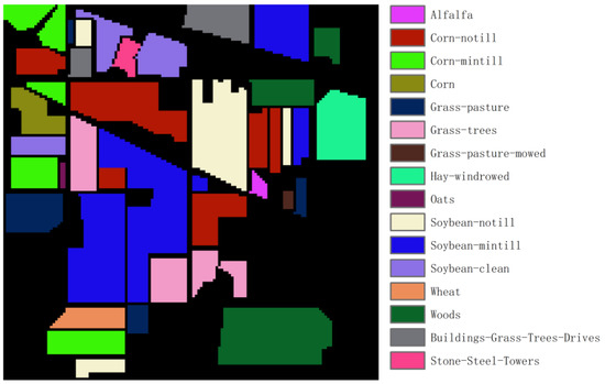
Figure 1.
Ground truth of the Indian Pines dataset.
Salinas: This dataset is a hyperspectral image acquired by the United States through AVIRIS, with a spatial resolution of 3.7 m. It contains 224 spectral bands, each with 512 × 217 pixels, and divides the ground objects into 16 categories, as shown in Figure 2. Due to the influence of covering the water absorption region, the 108–112, 154–167 and 224 bands were removed, and 204 bands were finally selected for the experiment.
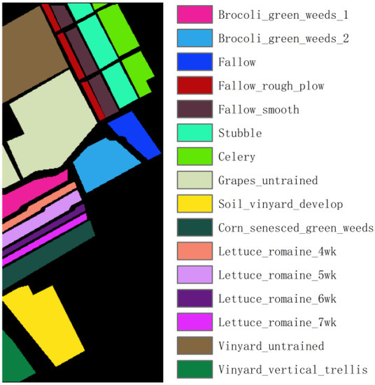
Figure 2.
Ground truth of the Salinas dataset.
KSC: This dataset was obtained by the United States through the AVIRIS satellite in 1996, with a spatial resolution of 18 m and a spectral range of 400–2500 nm. It contains 224 spectral bands, each with 512 × 614 pixels, and divides ground objects into 13 categories, as shown in Figure 3. Due to the influence of covering the water absorption region and its low signal-to-noise ratio, 176 bands were finally selected for experiments.
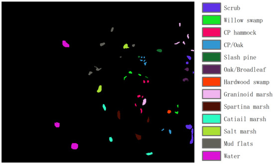
Figure 3.
Ground truth of the KSC dataset.
WHU-Hi-LongKou: This dataset is a hyperspectral image acquired by Wuhan University through Nano-Hyperspec on 17 July 2018, in Longkou Town, Hubei province, China, with a spatial resolution of 0.463 m and a spectral range of 400–1000 nm. It contains 270 spectral bands, each with 550 × 400 pixels, and divides ground objects into 9 categories, as shown in Figure 4.
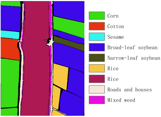
Figure 4.
Ground truth of the WHU-Hi-LongKou dataset.
2.2.2. Experimental Parameters
In the experiment, a machine learning classifier is used to supervise the classification of the hyperspectral images processed by the method. First, the selection and parameter setting of the machine learning classifier is carried out. The classifier used is random forest (RF). The experiment runs in Python and calls the sklearn library for classification. To reduce the difference in the classification effect of the method due to the parameters, the RF parameters use the default values as much as possible. The number of decision trees of RF is set to 100, and the impurity measure is set to Gini.
Next, the experimental parameters and evaluation indicators are chosen. To address potential overfitting issues and to provide a more robust evaluation of the method’s performance during classification, 10% of each category sample is randomly selected as training dataset, and the remaining 90% is used as test dataset. The final results take the average result of 20 method runs. At each run, the training and the test datasets are different. Since it is impossible to determine the optimal number of band selection methods on the four datasets, too few selected bands will lead to a limited amount of information being extracted by each band selection method; too many selected bands will lead to the same classification effect of different band selection methods. Therefore, the number of band selections in the experiment is from 5 to 50, with 5 as the step size for equal interval selection.
2.2.3. Evaluation Indicators
The experimental results of the experiment require appropriate evaluation indicators to evaluate the classification effect. The evaluation indicators selected in the experiment are overall accuracy (OA), average accuracy (AA), kappa (κ) and recall. OA is used to calculate the proportion of all correctly classified samples to the total samples from the overall point of view [34,35]. Kappa is the consistency measure of the actual and classification values, which can improve the OA shortcomings, ignoring the classification effect of categories with a small number of samples [36,37]. Combining the two evaluation indicators can obtain more reliable classification effect evaluation results. Recall is the ratio of the number of correctly classified samples among the samples of a specific category to the number of samples classified as this category, and the reliability of the classification effect is evaluated separately from the perspective of each category. AA accumulates and averages the recall of each category and evaluates the reliability of the classification effect of each category from an overall perspective [38,39].
The formula for calculating the OA is shown in (16).
In the formula, A represents the total number of samples; n represents the number of sample categories; and TPi represents the number of samples in category i, the actual value of which is positive and the classification value of which is positive.
The formula for calculating the kappa is shown in (17) and (18).
In the formula, p0 is OA and FPi represents the number of samples in category i, the actual value of which is positive and the classification value of which is negative.
The formula for calculating the recall is shown in (19).
In the formula, Recalli represents the recall of category i and FNi represents the number of samples in category i, the actual value of which is negative and the classification value of which is positive.
The formula for calculating the AA is shown in (20).
3. Evaluation Results
The experiment consists of two parts: the exploration and analysis of the classification effect of E-SR-SSIM and the exploration and analysis of the time efficiency of E-SR-SSIM. First, we explore and analyse the classification effect of the E-SR-SSIM method and SR-SSIM method on four datasets. Second, we compare and analyse the runtime of the E-SR-SSIM method and SR-SSIM method under four datasets.
3.1. Classification Effect of E-SR-SSIM
First, the difference in the classification effect between the E-SR-SSIM method combined with the modified threshold formula and the improved band subspace partition method and SR-SSIM is compared through experiments. The difference in the classification effect between the two methods is shown in Figure 5. Then, the classification effect of E-SR-SSIM and SR-SSIM in each object category is compared through experiments, and the recall is selected as the evaluation index of the classification effect. Among them, the number of selected bands for the Indian Pines and Salinas datasets is 10, and the number of selected bands for the KSC and WHU-Hi-LongKou dataset is 15. The classification effects of E-SR-SSIM and SR-SSIM for each object category on the four datasets are shown in Table 2, Table 3, Table 4 and Table 5.
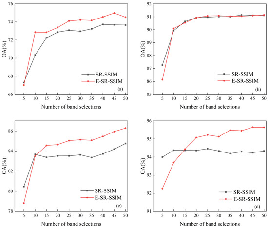
Figure 5.
Classification results of four datasets: (a) Indian Pines, (b) Salinas, (c) KSC and (d) WHU-Hi-LongKou.
Table 2.
Classification results of the Indian Pines dataset on 10 bands.
Table 3.
Classification results of the Salinas dataset on 10 bands.
Table 4.
Classification results of the KSC dataset on 15 bands.
Table 5.
Classification results of the WHU-Hi-LongKou dataset on 15 bands.
It can be seen in Figure 5 that with the increase in the number of bands in the four datasets, both E-SR-SSIM and SR-SSIM show the trend of an increasing classification effect. In particular, when the number of band selections ranges from 5 to 10, the classification performance of both E-SR-SSIM and SR-SSIM shows a significant step-up. Except for the small number of band selections, the classification effect of E-SR-SSIM is better than that of SR-SSIM, and the maximum improvements in the four datasets are 2.52%, 0.10%, 1.75% and 1.40%. E-SR-SSIM has better stability in the classification effect, and there is no decline in SR-SSIM when the number of band selections in the KSC dataset is 15.
Table 2 shows that for the Indian Pines dataset, E-SR-SSIM is better than SR-SSIM in the classification of most ground object categories, and 8 of the 16 categories have been improved. The improvement of E-SR-SSIM in OA, AA and kappa is 2.72%, 0.78% and 3.10%, respectively, and the most significant improvement of the ground object category is the improvement of Corn-mintill by 9.65%. E-SR-SSIM significantly improves the Oats with the worst classification effect of SR-SSIM from 5.00% to 9.72%, nearly doubling the classification effect. Since E-SR-SSIM has improved the category classification effect of large test samples, the AA of E-SR-SSIM has been improved.
It can be seen from Table 3 that for the Salinas dataset, E-SR-SSIM is better than SR-SSIM in the classification of most object categories, and 13 of the 16 categories improved. The improvement of E-SR-SSIM in OA, AA and kappa is 0.26%, 0.30% and 0.29%, respectively, and the most significant improvement of the ground object category is Vinyard_untrained by 1.38%. Since SR-SSIM has a better classification effect in the Salinas dataset, E-SR-SSIM does not improve the classification effect significantly, and the improvement in each surface object category is less than 2%.
Table 4 shows that for the KSC dataset, E-SR-SSIM is better than SR-SSIM in the classification of most object categories, and 9 of the 13 categories improved. E-SR-SSIM increases OA, AA and kappa by 2.38%, 3.06% and 2.66%, respectively, and the most significant increase in the ground object category is CP/Oak by 9.98%. In particular, it should be noted that all nine improved categories are categories with better classification effects in SR-SSIM, thus proving the superiority of E-SR-SSIM.
Table 5 shows that for the WHU-Hi-LongKou dataset, E-SR-SSIM is better than SR-SSIM in the classification of most object categories, and six of the nine categories improved. E-SR-SSIM increases OA, AA and kappa by 0.05%, 0.15% and 0.06%, respectively, and the most significant increase in the ground object category is Mixed weed by 4.86%. Due to the good classification performance of the SR-SSIM, the improvement in classification performance of the E-SR-SSIM is not significant in OA, AA and kappa.
3.2. Time Efficiency of E-SR-SSIM
Through experiments, it was found that compared with SR-SSIM, the improved band selection method E-SR-SSIM had no significant decline in the classification effect on the four datasets. In contrast, the classification effect remained flat or even slightly increased. Therefore, to ensure the classification effect, the running time of E-SR-SSIM and SR-SSIM on the four datasets can be compared through experiments to verify the effectiveness of the band subspace partition method to reduce the runtime of the method.
The experiment was run on a Windows 10 system, and the processor was an AMD Ryzen 7 5825U. The main frequency was 2.00 GHz, the effective memory was 32 GB and the development environment was Python 3.8. Comparing the running time of the SR-SSIM method and the E-SR-SSIM method on the four datasets, the specific results of the computational time are shown in Figure 6 and Table 6. The unit of Table 6 is seconds. Since the SR-SSIM method sorts all the bands in descending order according to the product results and selects the required number of bands, each band number of the SR-SSIM computational time was the same.
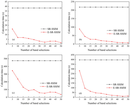
Figure 6.
Computational times of four datasets: (a) Indian Pines, (b) Salinas, (c) KSC and (d) WHU-Hi-LongKou.
Table 6.
The details of the computational times of the four datasets on the SR-SSIM and E-SR-SSIM mthod.
Figure 6 and Table 6 show that the computational time of E-SR-SSIM in each band is shorter than that of SR-SSIM, indicating that E-SR-SSIM can effectively reduce the computational time of the method while ensuring the classification effect; additionally, as the number of bands increases, the runtime of E-SR-SSIM also shows a downwards trend, indicating that as the number of subdatasets increases, the runtime of E-SR-SSIM is continuously decreasing.
Now, according to the method logic of E-SR-SSIM, the runtime of E-SR-SSIM on each band is shorter than that of SR-SSIM, and as the number of bands increases, the computational time of E-SR-SSIM also shows a declining trend. The reason is that the band subspace partition can remove SSIM calculation for different subdatasets, as shown in Figure 7. The band subspace partition makes the number of calculations inversely proportional to the number of subspaces, thereby reducing the calculation time of the method, so the runtime of E-SR-SSIM on each band is shorter than that of SR-SSIM. Moreover, E-SR-SSIM also shows a downwards trend with the increased number of bands.
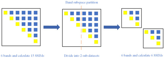
Figure 7.
Band subspace partition reduces SSIM. The yellow squares represent the two same bands and do not need to calculate the SSIM. The blue squares represent two different bands and need to calculate the SSIM.
4. Discussion
4.1. Band Subspace Partition Reduces SSIM Calculation
Through experiments, it is found that SR-SSIM takes more than 99% of the time to calculate SSIM. In Section 3.2, it can be concluded that the band subspace partition can reduce the SSIM calculation time, thereby reducing the method’s runtime. However, there needs to be a more quantitative analysis of the band subspace partition to reduce the number of SSIM calculations. In this subsection, through mathematical analysis, the quantitative proof that the band subspace partition reduces the calculation amount of SSIM is obtained, thereby reducing the running time of the E-SR-SSIM method.
Assuming a dataset has bands, the number of times to calculate SSIM is times. Divide this dataset into two subdatasets. The number of bands in the first subdataset is , and the number of bands in the other subdataset is . The number of times SSIM is calculated is times, and the number of calculations becomes the original . Since the coarse partition is divided into equal intervals and the fine partition is adjusted based on the coarse partition, it can be considered that the number of bands in the two subdatasets is approximately equal, that is, , and the number of calculations can be expressed as . When tends to , the number of calculations tends to be of the original. Similarly, it can be seen that when it is divided into subspaces as evenly as possible, the number of calculations tends to be of the original.
The experiments verify the above mathematical proof. The improved band subspace partition method is used on the four datasets of Indian Pines, Salinas, KSC and WHU-Hi-LongKou, and the time required for SSIM operation is recorded under different numbers of subspaces. The experimental results are shown in Figure 8. In Figure 8, the experimental results can generally be expressed as a curve in which the SSIM operation time decreases as the number of subspaces increases, which is in line with theoretical expectations.
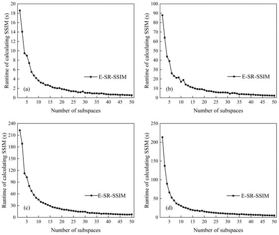
Figure 8.
Runtimes with different subspace numbers: (a) Indian Pines, (b) Salinas, (c) KSC and (d) WHU-Hi-LongKou.
4.2. Classification Effect of Different Band Subspace Partitions
The improved band subspace partition method is compared with the original subspace partition method, and the effectiveness of the improved band subspace partition method is verified through experiments. Since the SR-SSIM method cannot run on datasets with a small number of bands, it is necessary to use a modified similarity threshold formula on the SR-SSIM method to overcome this defect. Therefore, band selection uses the SR-SSIM method with a modified threshold formula to compare the classification effects of the two band subspace partition methods. On the Indian Pines, Salinas and KSC datasets, the original band subspace partition method and the improved band subspace partition method are used for supervised classification, and the classification effect is shown in Figure 9.
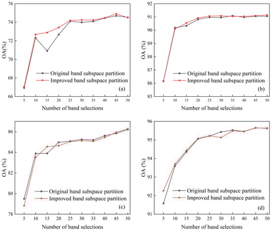
Figure 9.
Effectiveness of improved band subspace partition: (a) Indian Pines, (b) Salinas, (c) KSC and (d) WHU-Hi-LongKou.
Figure 9 shows that the improved band subspace partition method is not inferior to the original band subspace partition method in terms of the classification effect. Additionally, compared with the original band subspace partition method, the classification effect is more stable, and the classification effect does not appear to significantly decrease (for example, the number of bands in the Indian Pines dataset is 15). It shows that the improved band subspace partition method can scientifically group the bands. It corrects the defect that the original band subspace partition method does not consider the position of the previous partition points.
5. Conclusions
This paper proposes a band selection method, E-SR-SSIM, based on band subspace partition to solve the problem of existing band selection methods calculating many SSIMs, resulting in an excessively long runtime. The method first divides the dataset into subdatasets and dynamically adjusts the partition points according to the situation for each subdataset. Then, the SR-SSIM method is used to modify the similarity threshold formula for each subdataset to select the most representative band. Using the RF classifier for supervised classification on the Indian Pines, Salinas and KSC public datasets, the following three conclusions can be drawn: (1) The classification effect of the E-SR-SSIM method is roughly the same as that of the SR-SSIM method. (2) Compared with SR-SSIM, the E-SR-SSIM method can effectively reduce the method’s runtime while ensuring the classification effect. (3) The improved band subspace partition method is compared with the original method. The classification effect can be improved slightly and can maintain specific stability.
Although the E-SR-SSIM method reduces the runtime of the method while ensuring the classification effect compared with the SR-SSIM method, some shortcomings still need improvement. First, due to the number of bands in a subdataset needing to be greater than or equal to 3, the E-SR-SSIM could not select any number of bands. In subsequent work, the band sub-space partition method of the E-SR-SSIM should be improved. The new band subspace partition method could select any number of bands easily. Second, when the dataset has lots of noise, such as the Botswana dataset, the E-SR-SSIM would compulsorily divide the dataset into many subdatasets, ignoring the situation of the dataset. As a result, the classification effect of the E-SR-SSIM is inferior to that of the SR-SSIM. In other words, E-SR-SSIM is susceptible to noise bands. In subsequent work, the E-SR-SSIM should enhance its robustness to noise bands. Third, how to pre-process the dataset without discarding the robustness of the method is the object of our future work. Fourth, E-SR-SSIM needs to be compared with some recently developed band selection methods to illustrate its advantages. Fifth, the influence of different numbers of training samples on the classification effect of E-SR-SSIM should be analysed in future work and E-SR-SSIM should be improved based on those experimental results.
Author Contributions
Conceptualization, T.H. and P.G.; methodology, T.H.; validation, T.H.; formal analysis, T.H.; data curation, T.H.; writing—original draft preparation, T.H.; writing—review and editing, P.G., S.Y. and S.S.; project administration, T.H., P.G., S.Y. and S.S.; funding acquisition, T.H. and P.G. All authors have read and agreed to the published version of the manuscript.
Funding
This work was supported by a Second Tibetan Plateau Scientific Expedition and Research Program (grant No. 2019QZKK0608) and an Open Fund of the State Key Laboratory of Remote Sensing Science and Beijing Engineering Research Center for Global Land Remote Sensing Products (grant No. OF202304).
Data Availability Statement
The three public AVIRIS hyperspectral datasets can be downloaded from https://www.ehu.eus/ccwintco/index.php?title=Hyperspectral_Remote_Sensing_Scenes (accessed on 15 June 2023). The WHU-Hi-LongKou hyperspectral dataset can be downloaded from http://rsidea.whu.edu.cn/resource_WHUHi_sharing.htm (accessed on 14 July 2023).
Acknowledgments
The authors thank three anonymous reviewers for supporting the insightful comments.
Conflicts of Interest
The authors declare no conflict of interest.
References
- Gao, P.; Xie, Y.; Song, C.; Cheng, C.; Ye, S. Exploring detailed urban-rural development under intersecting population growth and food production scenarios: Trajectories for China’s most populous agricultural province to 2030. J. Geogr. Sci. 2023, 33, 222–244. [Google Scholar] [CrossRef]
- Wang, Y.; Song, C.; Cheng, C.; Wang, H.; Wang, X.; Gao, P. Modelling and evaluating the economy-resource-ecological environment system of a third-polar city using system dynamics and ranked weights-based coupling coordination degree model. Cities 2023, 133, 104151. [Google Scholar] [CrossRef]
- Gao, P.; Gao, Y.; Ou, Y.; McJeon, H.; Zhang, X.; Ye, S.; Wang, Y.; Song, C. Fulfilling global climate pledges can lead to major increase in forest land on Tibetan Plateau. iScience 2023, 26, 106364. [Google Scholar] [CrossRef] [PubMed]
- Lu, B.; Dao, P.D.; Liu, J.; He, Y.; Shang, J. Recent advances of hyperspectral imaging technology and applications in agriculture. Remote Sens. 2020, 12, 2659. [Google Scholar] [CrossRef]
- Duan, P.; Ghamisi, P.; Kang, X.; Rasti, B.; Li, S.; Gloaguen, R. Fusion of dual spatial information for hyperspectral image classification. IEEE Trans. Geosci. Remote Sens. 2020, 59, 7726–7738. [Google Scholar] [CrossRef]
- Dong, W.; Fu, F.; Shi, G.; Cao, X.; Wu, J.; Li, G.; Li, X. Hyperspectral image super-resolution via non-negative structured sparse representation. IEEE Trans. Image Process. 2016, 25, 2337–2352. [Google Scholar] [CrossRef]
- Rasti, B.; Scheunders, P.; Ghamisi, P.; Licciardi, G.; Chanussot, J. Noise reduction in hyperspectral imagery: Overview and application. Remote Sens. 2018, 10, 482. [Google Scholar] [CrossRef]
- Ghamisi, P.; Plaza, J.; Chen, Y.; Li, J.; Plaza, A.J. Advanced spectral classifiers for hyperspectral images: A review. IEEE Geosci. Remote Sens. Mag. 2017, 5, 8–32. [Google Scholar] [CrossRef]
- Lu, G.; Fei, B. Medical hyperspectral imaging: A review. J. Biomed. Opt. 2014, 19, 010901. [Google Scholar] [CrossRef]
- Heylen, R.; Parente, M.; Gader, P. A review of nonlinear hyperspectral unmixing methods. IEEE J. Sel. Top. Appl. Earth Obs. Remote Sens. 2014, 7, 1844–1868. [Google Scholar] [CrossRef]
- Hughes, G. On the mean accuracy of statistical pattern recognizers. IEEE Trans. Inf. Theory 1968, 14, 55–63. [Google Scholar] [CrossRef]
- Gao, P.; Wang, J.; Zhang, H.; Li, Z. Boltzmann entropy-based unsupervised band selection for hyperspectral image classification. IEEE Geosci. Remote Sens. Lett. 2018, 16, 462–466. [Google Scholar] [CrossRef]
- Gao, P.; Zhang, H.; Wu, Z.; Wang, J. A joint landscape metric and error image approach to unsupervised band selection for hyperspectral image classification. IEEE Geosci. Remote Sens. Lett. 2021, 19, 1–5. [Google Scholar] [CrossRef]
- Zhang, H.; Wu, Z.; Wang, J.; Gao, P. Unsupervised band selection for hyperspectral image classification using the Wasserstein metric-based configuration entropy. Acta Geod. Cartogr. Sin. 2021, 50, 405–415. [Google Scholar]
- Wang, Q.; Lin, J.; Yuan, Y. Salient band selection for hyperspectral image classification via manifold ranking. IEEE Trans. Neural Netw. Learn. Syst. 2016, 27, 1279–1289. [Google Scholar] [CrossRef]
- Uddin, M.P.; Mamun, M.A.; Afjal, M.I.; Hossain, M.A. Information-theoretic feature selection with segmentation-based folded principal component analysis (PCA) for hyperspectral image classification. Int. J. Remote Sens. 2021, 42, 286–321. [Google Scholar] [CrossRef]
- Xu, Y.; Zhang, L.; Du, B.; Zhang, F. Spectral-spatial unified networks for hyperspectral image classification. IEEE Trans. Geosci. Remote Sens. 2018, 56, 5893–5909. [Google Scholar] [CrossRef]
- Zhu, M.; Jiao, L.; Liu, F.; Yang, S.; Wang, J. Residual spectral-spatial attention network for hyperspectral image classification. IEEE Trans. Geosci. Remote Sens. 2020, 59, 449–462. [Google Scholar] [CrossRef]
- Wang, Q.; Zhang, F.; Li, X. Optimal clustering framework for hyperspectral band selection. IEEE Trans. Geosci. Remote Sens. 2018, 56, 5910–5922. [Google Scholar] [CrossRef]
- Wang, Q.; Li, Q.; Li, X. A fast neighborhood grouping method for hyperspectral band selection. IEEE Trans. Geosci. Remote Sens. 2020, 59, 5028–5039. [Google Scholar] [CrossRef]
- Sun, H.; Zhang, L.; Ren, J.; Huang, H. Novel hyperbolic clustering-based band hierarchy (HCBH) for effective unsupervised band selection of hyperspectral images. Pattern Recognit. 2022, 130, 108788. [Google Scholar] [CrossRef]
- Wang, Z.; Bovik, A.C.; Sheikh, H.R.; Simoncelli, E.P. Image quality assessment: From error visibility to structural similarity. IEEE Trans. Image Process. 2004, 13, 600–612. [Google Scholar] [CrossRef] [PubMed]
- Gao, Y.; Rehman, A.; Wang, Z. CW-SSIM Based Image Classification. In Proceedings of the 2011 18th IEEE International Conference on Image Processing, Brussels, Belgium, 11–14 September 2011; pp. 1249–1252. [Google Scholar]
- Renieblas, G.P.; Nogués, A.T.; González, A.M.; Gómez-Leon, N.; Del Castillo, E.G. Structural similarity index family for image quality assessment in radiological images. J. Med. Imaging 2017, 4, 035501. [Google Scholar] [CrossRef] [PubMed]
- Moghimi, A.; Mohammadzadeh, A.; Celik, T.; Amani, M. A novel radiometric control set sample selection strategy for relative radiometric normalization of multitemporal satellite images. IEEE Trans. Geosci. Remote Sens. 2020, 59, 2503–2519. [Google Scholar] [CrossRef]
- Chan, J.C.-W.; Ma, J.; Kempeneers, P.; Canters, F. Superresolution enhancement of hyperspectral CHRIS/Proba images with a thin-plate spline nonrigid transform model. IEEE Trans. Geosci. Remote Sens. 2010, 48, 2569–2579. [Google Scholar] [CrossRef]
- Qiao, T.; Ren, J.; Sun, M.; Zheng, J.; Marshall, S. Effective compression of hyperspectral imagery using an improved 3D DCT approach for land-cover analysis in remote-sensing applications. Int. J. Remote Sens. 2014, 35, 7316–7337. [Google Scholar] [CrossRef]
- Jia, S.; Zhu, Z.; Shen, L.; Li, Q. A two-stage feature selection framework for hyperspectral image classification using few labeled samples. IEEE J. Sel. Top. Appl. Earth Obs. Remote Sens. 2013, 7, 1023–1035. [Google Scholar] [CrossRef]
- Ghorbanian, A.; Maghsoudi, Y.; Mohammadzadeh, A. Clustering-Based Band Selection Using Structural Similarity Index and Entropy for Hyperspectral Image Classification. Trait. Signal 2020, 37, 785–791. [Google Scholar] [CrossRef]
- Xu, B.; Li, X.; Hou, W.; Wang, Y.; Wei, Y. A similarity-based ranking method for hyperspectral band selection. IEEE Trans. Geosci. Remote Sens. 2021, 59, 9585–9599. [Google Scholar] [CrossRef]
- Rodriguez, A.; Laio, A. Clustering by fast search and find of density peaks. Science 2014, 344, 1492–1496. [Google Scholar] [CrossRef]
- Lu, Y.; Ren, Y.; Cui, B. Noise robust band selection method for hyperspectral images. J. Remote Sens. 2022, 26, 2382–2398. [Google Scholar] [CrossRef]
- Wang, Q.; Li, Q.; Li, X. Hyperspectral band selection via adaptive subspace partition strategy. IEEE J. Sel. Top. Appl. Earth Obs. Remote Sens. 2019, 12, 4940–4950. [Google Scholar] [CrossRef]
- Zhou, L.; Ma, X.; Wang, X.; Hao, S.; Ye, Y.; Zhao, K. Shallow-to-Deep Spatial–Spectral Feature Enhancement for Hyperspectral Image Classification. Remote Sens. 2023, 15, 261. [Google Scholar] [CrossRef]
- Zhang, J.; Zhao, L.; Jiang, H.; Shen, S.; Wang, J.; Zhang, P.; Zhang, W.; Wang, L. Hyperspectral Image Classification Based on Dense Pyramidal Convolution and Multi-Feature Fusion. Remote Sens. 2023, 15, 2990. [Google Scholar] [CrossRef]
- Wang, X.; Wang, J.; Lian, Z.; Yang, N. Semi-Supervised Tree Species Classification for Multi-Source Remote Sensing Images Based on a Graph Convolutional Neural Network. Forests 2023, 14, 1211. [Google Scholar] [CrossRef]
- Wang, B.; Zhou, M.; Cheng, W.; Chen, Y.; Sheng, Q.; Li, J.; Wang, L. An Efficient Cloud Classification Method Based on a Densely Connected Hybrid Convolutional Network for FY-4A. Remote Sens. 2023, 15, 2673. [Google Scholar] [CrossRef]
- Yang, H.; Chen, M.; Wu, G.; Wang, J.; Wang, Y.; Hong, Z. Double Deep Q-Network for Hyperspectral Image Band Selection in Land Cover Classification Applications. Remote Sens. 2023, 15, 682. [Google Scholar] [CrossRef]
- Alkhatib, M.Q.; Al-Saad, M.; Aburaed, N.; Almansoori, S.; Zabalza, J.; Marshall, S.; Al-Ahmad, H. Tri-CNN: A three branch model for hyperspectral image classification. Remote Sens. 2023, 15, 316. [Google Scholar] [CrossRef]
Disclaimer/Publisher’s Note: The statements, opinions and data contained in all publications are solely those of the individual author(s) and contributor(s) and not of MDPI and/or the editor(s). MDPI and/or the editor(s) disclaim responsibility for any injury to people or property resulting from any ideas, methods, instructions or products referred to in the content. |
© 2023 by the authors. Licensee MDPI, Basel, Switzerland. This article is an open access article distributed under the terms and conditions of the Creative Commons Attribution (CC BY) license (https://creativecommons.org/licenses/by/4.0/).