Classification of Marine Sediment in the Northern Slope of the South China Sea Based on Improved U-Net and K-Means Clustering Analysis

Abstract

The classification of marine sediment based on acoustic data is crucial for various applications such as marine resource exploitation, marine engineering construction, and marine ecological environment maintenance. It serves as a valuable alternative to limited geological sampling. However, the accuracy of sediment classification is limited due to constraints in acoustic data detection methods, data quality, and classification techniques. To address this issue, this study proposes an automatic classification method for marine sediment using an improved U-convolutional neural network and K-means clustering algorithm. In the coding part, a spatial pyramid pool layer is introduced to fuse low-dimensional feature data of different scales with the features of each level of the corresponding coding layer. This fusion method enhances the accuracy of the constructed relationship between the physical property parameters of the seabed bottom. The K-means clustering algorithm is optimized through selecting the point at the density center as the initial clustering center during the initial clustering center selection stage. This approach solves the sensitivity problem of the initial clustering center of K-means, improves the edge extraction effect of sediment types, and enhances the classification accuracy of sediment types. To validate the proposed method, an application test is conducted in the Northern Slope area of the South China Sea. The mean grain size of sediments in the study area is predicted using the improved U-Net neural network and the seafloor reflection intensity of the sub-bottom profile. Compared to the standard U-Net network results, the mean grain size prediction results show an increase of 4.9% and 2.8%, respectively. The sediment with the predicted mean grain size is then classified using the K-means clustering algorithm, resulting in the division of five sediment types: gravelly sand, sand, silty sand, sandy silt, and clayey silt. These classifications align well with the South China Sea sediment type map. The findings of this study not only provide an important supplement to existing marine sediment classification methods but also contribute significantly to understanding the sedimentary environment and processes in the Northern Slope of the South China Sea.

1. Introduction

The classification of sediments on the seafloor is a crucial aspect of ocean exploration and is essential for the development of marine resources, construction of marine engineering, and maintenance of the marine ecological environment. The use of acoustic data for marine sediment classification is in line with the modern concept of sustainable development and is more automated and intelligent than the conventional mechanical sediment sampling method. This method has a vast research scope and application prospects. In 1999, Hamilton et al. conducted a comparative study on the classification performance of RoxAnn and QTC-View classification software [1]. Preston et al. investigated the correlation between relevant parameters of submarine rock and soil and sediment acoustics [2]. In 2000, Tegowski analyzed the fractal characteristics of echo signals [3]. In 2001, Preston obtained backscattering data of marine sediments from shallow sea areas, performed principal component analysis on nearly 130 characteristic quantities, and selected the optimal features for sediment classification to identify fine sediment types on the seafloor [4,5]. In 2010, Giovanni et al. explored the relationship between sounding data, scattering intensity data, and the angular response of scattering intensity and sediment granularity, distribution of seafloor grasses, and relative scattering intensity threshold of five types of sediments, including gravel, gravel sand, and argillaceous sand with a small amount of gravel [6]. In 2013, Wienberg et al. utilized multi-beam sonar technology to scan the Coral Patch seamount which is located in the NE Atlantic Ocean half-way between the Iberian Peninsula and Madeira and classify the sediments [7]. Currently, multi-beam backscattering intensity data are the primary method for marine sediment classification. This method is effective at classifying gravel, sand, clay, and other types, but it faces challenges in achieving ideal results when the sediment differences are small.

Sub-bottom profiling is a widely used technique for exploring submarine stratigraphy based on acoustic principles. The geological interpretation of sub-bottom profiles is based on echo characteristics and morphology. This technique is commonly used in preliminary geological investigations for offshore wind power site surveys, submarine routing pipeline laying, and other offshore engineering constructions due to its high detection resolution, fast and convenient nature, and low cost [8,9,10,11]. However, conventionally engineered geological exploration processes the sub-bottom profile in a simple manner, resulting in low data utilization, low interpretation accuracy and precision, and other issues [12,13]. Recently, the inversion of marine sediment properties using sub-bottom profile data has emerged as a new way of implementing sub-bottom profile data for sediment classification. Chirp sub-bottom profile data have been successfully used to quantify the physical property parameters of shallow sediments on the seafloor. Statistical analysis of chirp profiles and sediment test data has been used to analyze the distribution patterns and deposition processes of surface sediments (Generally, the depth is in the range of 1 m) and sedimentation processes [14]. Inversion of the particle size, sediment type, and other properties of surface sediments have been investigated using chirp sonar data [15,16]. The parameters obtained were highly consistent with laboratory findings. Genetic algorithms have been applied to sub-bottom profiles to obtain impedance profiles, successively obtaining geological engineering parameters based on the empirical relationship between wave impedance and sediment mechanical properties [17].

In recent years, convolutional neural networks (CNNs) based on deep learning methods have been extensively used in various fields such as object detection, face recognition, and text classification [18,19,20]. It has become a research trend to apply CNN methods for the inversion of seafloor physical property parameters and sediment classification. Berthold et al. used side-scan sonar data and GoogLeNet to preliminarily classify gravel, mud, sand, and mixed sediment [21]. Luo et al. compared the classification performance of deep and shallow CNN models for three types of sediment, namely stone, mud, and sand, and found that the shallow CNN model outperformed the deep CNN model while achieving excellent classification performance [22]. Wang et al. conducted a study on sediment classification using MSC-Transformer and shallow formation profile data and achieved good results [23]. Additionally, Tegowski extracted features such as fractal dimension and spectral length of backscatter images as K-means clustering parameters for classification [24]. Lu Liang et al. used texture features and the K-means clustering algorithm to classify marine sediments and determine the optimal number of classifications [25].

The U-Net network was initially developed for semantic segmentation tasks in medical imaging and has shown promising results [26]. Compared to other existing semantic segmentation models, U-Net is a compact model with fewer training parameters, specifically designed for scenarios with limited training samples. These characteristics make U-Net a commonly used model for various semantic segmentation tasks [27,28]. Unsupervised classification, also known as cluster analysis, is a valuable technique for extracting structural information from sample data. It has found extensive applications across various fields, leading to the development of numerous algorithms. Some commonly employed algorithms include hierarchical clustering, the K-means algorithm, the self-organizing map (SOM) network, and the attractor propagation algorithm [29,30].

As we all know, the Northern Slope region of the South China Sea is a complex topographical area with a series of submarine canyons [31,32] and a water depth ranging from 400 m to 2500 m. The shallow-water-area sediments are mainly silty clay and silty sand, while the deep-water-area sediments with water depth greater than 1000 m are mainly fine-grained clay and silty clay [33]. This paper proposes an automatic classification method for marine sediment types in the Northern Slope of the South China Sea using an improved U-Net and K-means clustering algorithm. The method utilizes multibeam bathymetry, topographic slope, reflection intensity of the sub-bottom profile, and sample test data to predict the mean grain size of the seafloor. A U-Net network model with low dimensional feature retention and pooled index sampling is established to achieve this prediction. An optimized K-means clustering algorithm is then used to classify sediment types. In the initial clustering center selection stage, the edge extraction effect of sediment types is optimized through comparing the error squares and searching the density center as the initial clustering center, which improves the classification accuracy of marine sediment types [34]. The classification results are analyzed comprehensively with the geological background and sediment distribution characteristics of the study area to further divide the sedimentary environment of the study area and explore the distribution rule and sedimentary characteristics of the study area. This provides data support for the understanding of the sedimentary environment and sedimentary process of the Northern Slope of the South China Sea and has important practical significance for the development of nearby resources.

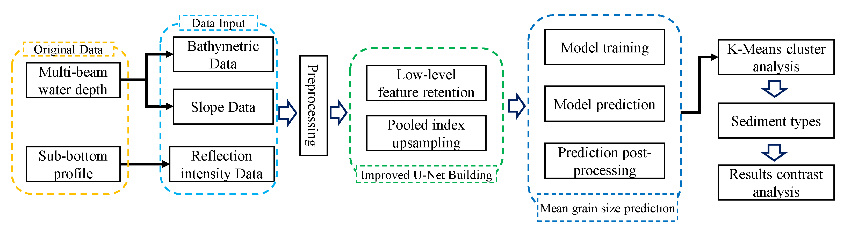
2. Data and Methods

2.1. Data Collection

2.1.1. Multibeam Survey

The present study utilizes a dataset comprising of multibeam bathymetry, topographic slope, seafloor reflection intensity (based on sub-bottom profiling data), and mean grain size data obtained from sampling tests in the study area. The multibeam bathymetric data were collected in 2011 as part of an investigation using the multibeam bathymetry system on board the survey vessel ‘South Sea 503’. The collected data were subsequently processed using Caris HIPS and SIPS (Version: 11.4.12) software, which is a widely used software in the field of marine hydrography. Caris HIPS is capable of processing multibeam bathymetric data and generating high-precision terrain information and bathymetric charts. The software applies various processing steps, including calibration, filtering, and compensation, to the raw multibeam bathymetric data in order to produce clear and accurate bathymetric charts. The processed data undergoes tide correction, draft correction, sound velocity correction, and error correction, followed by merging and coordinate conversion. A DTM data grid of 20 m × 20 m is then constructed. The water depth data and terrain slope data are output after editing and processing.

2.1.2. Sub-Bottom Profiling

The acquisition of sub-bottom profile data was facilitated through the use of the Ixsea Echoes 3500 sub-bottom profiler. This device is specifically designed to utilize sound waves for the detection of geological and topographical features, thereby providing information about sub-bottom structures. In 2011, the survey vessel ‘South Sea 503’ utilized this instrument to conduct measurements and gather sub-bottom profiles in the study area. The obtained sub-bottom profile data were subsequently processed using Triton SB-Interpreter, a software platform developed by TRITON IMAGINE. Triton Interpreter is specifically designed for the processing of shallow seismic profile data. It facilitates the interpretation, analysis, and visualization of these data, thereby assisting researchers in obtaining a comprehensive understanding of the geological characteristics of sub-bottom structures. The processing includes channel head processing, bandpass filtering processing, amplitude gain, etc. The sea-bottom reflection intensity value is extracted based on the processed shallow formation section data. Kriging interpolation is employed to generate regional seafloor reflection intensity data. In sub-bottom profiles, the interface between seawater and the seafloor is observed as the first strong positive polarity reflection, as depicted in Figure 1a,b. The intensity of this reflection is determined by the acoustic impedance and acoustic reflection coefficient at the seabed. The reflection coefficient and acoustic impedance are closely linked to the physical properties of the sediment, such as mean grain size [17], shown in Figure 1c. Therefore, the sub-bottom profile data contains valuable information about the physical properties of marine sediment. It is possible to study the relationship between the relevant acoustic properties and physical properties of the soil in the sub-bottom profile data. An inversion method for determining the physical property parameters of sediments based on the sub-bottom profile data has been established.

2.1.3. Sediment Sampling

The geological sampling test data are mainly gravity corer sampling test data provided by COSL Engineering Investigation Center, a cooperation unit of the previous project. Some stations are quoted from the box corer sediment samples obtained by Zhu Chaoqi of Ocean University of China [35]. In June 2015, the box corer sediment samples were obtained by the “Experiment 3” research ship.

Figure 2 depicts the location of the study area, sub-bottom profile lines, and sampling stations. The research area is covered by 36 sub-bottom profile lines, with a minimum line spacing of 400 m and a maximum of 2000 m. The sampling stations are sparsely distributed throughout the region, totaling 41. Based on the analysis of the collected data, the marine sediment types in the study area can be classified into five types.

The distribution characteristics of water depth, slope, and seafloor reflection intensity in the study area are presented in Figure 3.

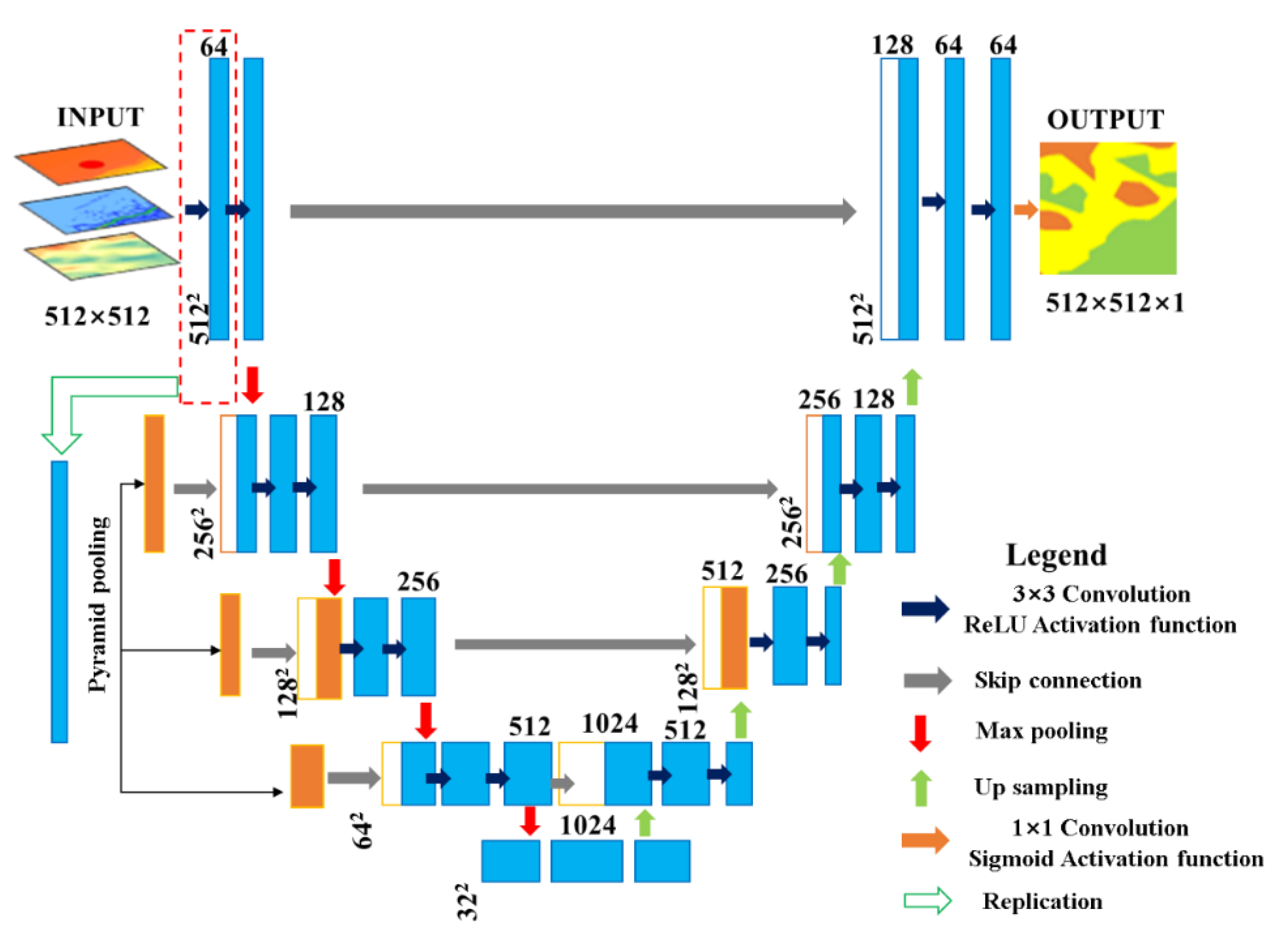
2.2. Improved U-Net

The U-Net network architecture consists of an encoder and a decoder with encoder symmetry structure. The encoder is responsible for obtaining semantic information, while the decoder performs the processes of downsampling and upsampling of data. The decoder uses a typical convolutional network structure, which alternates between multi-layer convolution and pooling operations to gradually reduce the resolution of feature data and double the number of channels of feature data at each layer. To obtain global information about the data, each step in the decoder corresponds to the encoder, including the upsampling of the feature data followed by multiple convolutions. The decoder gradually improves the resolution of the output feature data while reducing the number of channels of the feature data by half. To locate the upsampled features, the decoder splices them with feature data of the same resolution from the decoder via skip connections. However, with the deepening of the network, low-dimensional details of the input data are weakened after multiple convolution operations, and the computational effect of the edge contour of the data volume cannot be guaranteed. To address this issue, the spatial pyramid pool layer is introduced into the coding part of the network to preserve low-level features. The pyramid pooling layer reduces the low-dimensional feature data volume of the first convolution layer of U-Net to 1/2, 1/4, and 1/8 of the original size, and then performs feature fusion with the corresponding scale levels through dimension superposition.

Pooling is a crucial process for extracting features from data. It enables the optimal utilization of data information and storage resources through eliminating redundant information and preserving essential information. This, in turn, reduces the number of calculation parameters while ensuring accuracy. The pyramid pooling technique is based on multi-scale pooling, as illustrated in Figure 4. At the top of the pyramid, global averaging pooling is employed to extract the global context characteristics of the input. Initially, the input data are fed into a convolutional layer, resulting in a low-dimensional feature data body of size 512 × 512 × 64. Subsequently, maximum pooling is performed with pooling window sizes of 2 × 2, 4 × 4, and 8 × 8. The proposed method involves the utilization of global average pooling to extract local features of varying sizes within sub-regions. Subsequently, a 1 × 1 convolution is employed to reduce the dimensionality of the extracted features, thereby minimizing computational requirements. Finally, the pooling outcomes of different sizes are upsampled to match the dimensions of the input feature graph, and channel superposition fusion is performed to generate the ultimate output of the pyramid pooling module. The resulting low-dimensional feature data are then pyramided, resulting in feature data of sizes 256 × 256 × 64, 128 × 128 × 64, and 64 × 64 × 64. To ensure that each coding layer contains both detailed information of low-dimensional features and abstract high-dimensional features, the low-dimensional feature data of different scales are fused with the features of each level of the corresponding coding layer through dimensional superposition. This approach enables the establishment of a more accurate relationship between the physical property parameters of marine sediment.

To enhance the extraction of marine sediment type edges, a pooled index upsampling technique is employed in the decoding layer. Initially, the encoder conducts convolution and max pooling operations, where the position of the corresponding max pooling index is stored. Subsequently, the decoder performs upsampling and convolution, and each pixel is sent to the classifier. During the upsampling process, the corresponding max pooling index from the encoder layer is retrieved to perform upsampling. In comparison to the conventional U-Net’s deconvolution upsampling method, the pooled index upsampling technique sharpens the image edges, obviating the need for learning upsampling and reducing the network training parameters.

The improved U-Net architecture is depicted in Figure 5, which utilizes the U-shaped symmetrical structure of the standard U-Net. The network is composed of three parts, namely, downsampling, upsampling, and a skip connection structure. The encoder, located on the left side of Figure 4, performs compression through reducing the image size and extracting the feature map using two repeated convolution layers and one pooling layer. The convolution layer in the compression path (encoding layer) has a convolution kernel size of 3 × 3, and the rectified linear unit function is used as the activation function in the network. After the first convolution, the image retains low-level features through spatial pyramid pooling operation. The feature map obtained from the first convolution layer (conv1_1) is reduced to 1/2, 1/4, and 1/8 of the original size and then fused with pool1_3, pool2_4, and pool3_4, respectively. The pooling operation of the network combines max pooling and record indexing. In the decoder, located on the right side of Figure 4, the size of the last convolutional kernel in each decoding layer is halved to ensure that the feature map during upsampling has the same number of dimensions as the one after pooling in the encoding layer. Nonlinear upsampling of the feature map is then performed with the pooling index, as described by Vijay et al. [36].

Figure 6 illustrates the classification process of marine sediment in the Northern Slope area of the South China Sea. Initially, the original multibeam bathymetry and shallow formation profile data are processed to generate a dataset of seafloor depth, slope, and reflection intensity. Subsequently, the training set and the test set are obtained through matching positioning and image clipping of the sampled test data. The U-Net network structure is enhanced through incorporating a spatial pyramid pool layer in the coding part and utilizing the pool layer index sampling in the decoding part. The improved network model is trained, and the preliminary classification of the sediment type is performed. Finally, the K-means clustering analysis algorithm is employed to optimize the edge extraction effect of the sediment type, leading to further classification results.

Utilizing processed data on water depth, slope, and reflection intensity of sub-bottom profiles, a training and testing dataset was constructed in conjunction with sediment sampling data from the study area, as presented in

Table 1. Training dataset (TrD) and testing dataset (TtD).

Sediment Types	Water Depth (m)	Slope (°)	SBP Reflection Intensity (db)	Mean Grain Size (Φ)	Dataset	Label
Gravelly sand	255	1.28	0.62	5.45	TrD	0
	207	0.48	1.61	5.05	TtD
Sand	259	0.75	0.54	5.58	TrD	1
	508	0.92	0.33	5.96
	213	0.52	0.49	5.56	TtD
	533	2.62	0.34	5.64
Silty sand	580	0.98	0.36	6.17	TrD	2
	628	0.91	0.25	6.11
	543	1.70	0.33	6.38	TtD
	680	1.17	0.27	6.20
Sandy silt	864	3.24	0.18	6.47	TrD	3
	803	6.75	0.23	6.64
	1009	5.72	0.12	6.64
	912	3.12	0.21	6.88
	711	2.29	0.23	5.88
	849	1.68	0.21	6.64	TtD
	830	4.21	0.18	6.80
	689	1.78	0.24	6.06
Clayey silt	1227	1.06	0.08	7.06	TrD	4
	1413	1.30	0.09	7.38
	1405	4.17	0.09	7.01
	1431	3.47	0.11	6.98
	1455	1.83	0.11	6.72
	1383	3.67	0.07	6.97
	1408	2.55	0.07	6.88
	1323	3.39	0.10	6.97
	1300	3.67	0.07	6.64
	1192	5.28	0.09	6.64
	1183	6.15	0.10	6.80
	1088	1.65	0.11	6.74
	1066	3.23	0.13	7.08
	1084	1.61	0.12	6.72
	1060	7.23	0.14	7.38
	1023	6.74	0.15	7.64
	953	1.33	0.17	6.16
	1199	2.98	0.05	6.81	TtD
	1337	2.98	0.09	6.97
	1302	2.04	0.07	6.80
	1204	0.75	0.09	6.72
	965	5.57	0.18	6.64
	1276	1.56	0.09	6.84

. This dataset encompasses five distinct types of marine sediment, including gravelly sand, sand, silty sand, sandy silt, and clayey silt. The training data were utilized in the development of a network model, which established correlations between water depth, slope, reflection intensity, average particle size, and sediment type. This model was subsequently employed in the experiment of classifying marine sediment types.

2.3. Optimized K-Means Clustering Algorithm

The K-means algorithm is a widely used clustering algorithm in the field of data mining and knowledge discovery [37]. It is based on partition and is known for its simplicity of thought and fast convergence speed. The algorithm is an iteration-based repartition strategy that divides a given dataset into K cluster classes. During the iterative process, the Euclidean distance between each data point and the clustering center is optimized. The data point set X = {x₁, …, x_N} is partitioned into K clusters {C₁, …, C_K} represented by K partition centers ${\left\{X_l\right\}}^{K}l=1:K$. The objective function of the algorithm can be expressed as follows:

$$E={\sum }_{l=1}^K{\sum }_{x_i\in x_l}{‖x_i-C_l‖}^2$$

(1)

The K-means algorithm is a clustering method that aims to minimize a given objective function. The algorithm iteratively seeks the minimum value of the objective function. The basic K-means algorithm involves three steps:

• Initialization: The algorithm starts by dividing all samples into K initial clusters.
• Classification: Each sample in the dataset is assigned to the cluster with the closest center (mean). The distance between samples is typically calculated using Euclidean distance, either with standardized or non-standardized data. After classification, the centers of the clusters are recalculated based on the samples assigned to each cluster.
• Iteration: Step 2 is repeated until no further sample can be reassigned to a different cluster.

It is worth noting that Step 1 can also begin with a specified set of K initial centers, rather than dividing the samples into K initial clusters.

The traditional K-means algorithm generates initial clustering centers randomly, which can result in unstable clustering outcomes, causing the same dataset to produce different clustering results. This algorithm is highly sensitive to the initial clustering center, as the clustering centers randomly selected in the early stage of the algorithm may be isolated points or several points of the same class. The quality of clustering results is affected if the initial clustering center is not selected appropriately. The objective function J of the K-means algorithm calculates the sum of squares of minimized errors, and its formula is as follows:

$$J={\sum }_{m=1}^k{\sum }_{i=1}^{n}d(x_i,O_k)$$

(2)

Here, k represents the total number of subsets divided, Ok is the clustering center of the KTH cluster, and d(x_i, O_k) represents the distance between the data sample of the KTH cluster and the clustering center. The calculated sum of squares of error can only reach the minimum when the selected clustering center is located in the density center of the dataset. Therefore, this paper proposes an optimized K-means clustering algorithm based on this principle. In the initial clustering center selection stage, the point at the density center is found as the initial clustering center through comparing the sum of squares of error, which solves the sensitivity of the initial clustering center of K-means. During the clustering process, the same area projection method is used to project the structural plane onto the unit circle plane, and the Euclidean distance of two-dimensional points is used as the similarity measure of the structural plane. The optimization algorithm has the advantages of easy programming, few iteration times, stable clustering results, and so on. It has a good effect when applied to the classification of marine sediment.

The following is a detailed description of the method:

• For each data sample in the dataset, consider it as a potential clustering center and calculate its corresponding sum of squared errors. Select the data vector with the smallest sum of squared errors as the first initial clustering center.
• Based on the existing clustering centers, calculate the average sum of squared errors ($\overline{J}$) for the current dataset.

  $$\overline{J}=\frac{1}{k}{\sum }_{i=1}^k\left(\frac{1}{n}{\sum }_{m=1}^n{d}^2(x_j,k_i)\right)$$

  (3)
• To select the next initial clustering center, calculate the sum of squared errors that can be reduced when each data sample is considered as a potential clustering center. For a data sample (x_i, y_i) as a potential clustering center, the expression is:

  $$deJ=\overline{J}-({\left(x_j-x_i\right)}^2+{(y_j-y_i)}^2)$$

  (4)

Only when deJ > 0, the sum of squared errors can be reduced. The sum of reduced errors is denoted as sumdeJ.

$$sumdeJ={\sum }_{x_j\in D}deJ$$

(5)

Select the data sample with the maximum sumdeJ value as the next initial clustering center and add it to set U. Repeat Step 2 until all clustering centers are found. When selecting a clustering center from the set D and adding it to U, the chosen center X_i should be removed from the data sample set D.

3. Results

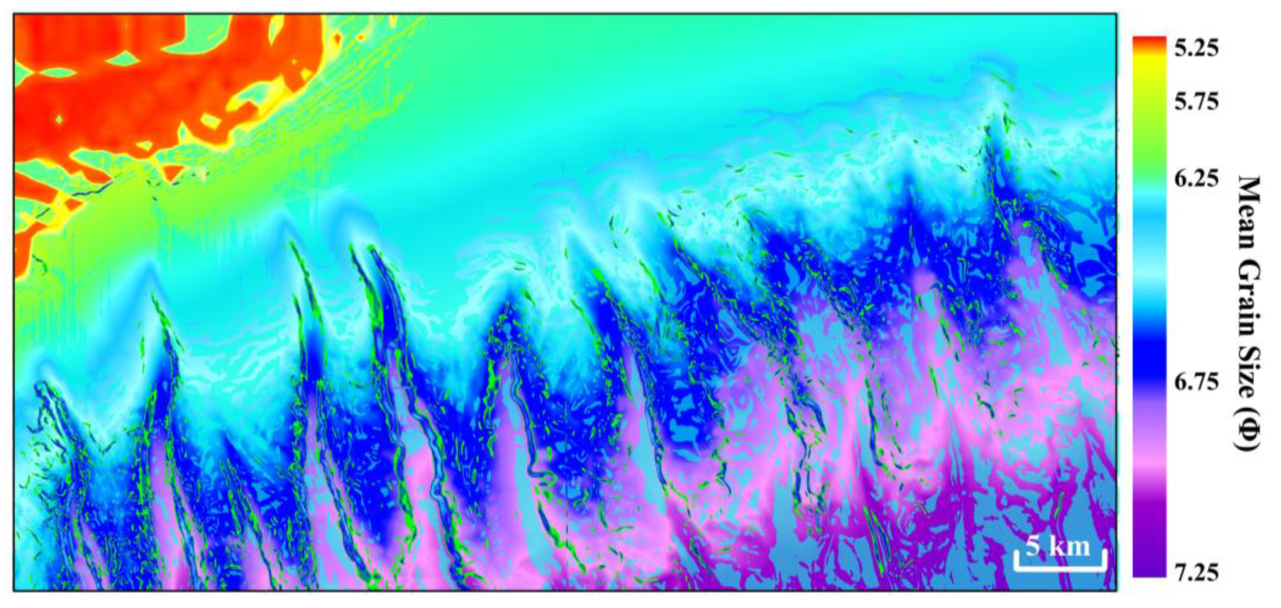
3.1. Improved U-Net Classification

The improved U-Net model utilizes a fully supervised learning approach, which necessitates the manual labeling of sample labels for marine sediment type in conjunction with sediment sampling data, as presented in Table 1. To account for the enhanced computing capability and spatial characteristics of the U-Net network, the original training dataset is randomly trimmed to a size of 512 × 512 using OpenCV open-source library programming through the Python language. Additionally, the following data augmentation techniques are applied to the dataset [38]: (1) rotation of the original data and corresponding label data by 90°, 180°, and 270°, respectively; (2) mirroring of the original data and corresponding label data along the Y-axis; (3) Gaussian fuzzy operation on the original data; (4) light adjustment to the original data; (5) addition of Gaussian noise and salt and pepper noise to the original data. After the data augmentation process, the training dataset comprises 1440 512 × 512 data blocks. Furthermore, to reduce training costs and obtain robust results, the transfer learning strategy proposed by Kumar et al. [39] is adopted in this study to fine-tune the existing network parameters, enabling the network to output high-level visual features that are robust and suitable for sediment type identification.

In this experiment, the batch size was set to 32, the epoch to 50, and the iteration times to 1000. The cross-entropy loss function was used as the objective function for the training network, with a learning rate of 0.1 and momentum of 0.9. The Stochastic Gradient Descent algorithm [40] was employed to minimize the objective function and obtain the optimal model. The method of cross-checking was adopted to obtain the optimal test results for the parameters set in this paper [41]. Figure 7 illustrates the changes in learning accuracy and loss value during the training process. The learning accuracy and loss value gradually decreased at around 200 iterations, and the improved U-Net model gradually converged. Subsequently, the trained improved U-Net was used to classify sediment in the test datasets, with the range of each pixel within [0, 1]. Finally, the prediction results were processed to obtain the mean grain size of the marine sediment, as shown in Figure 8.

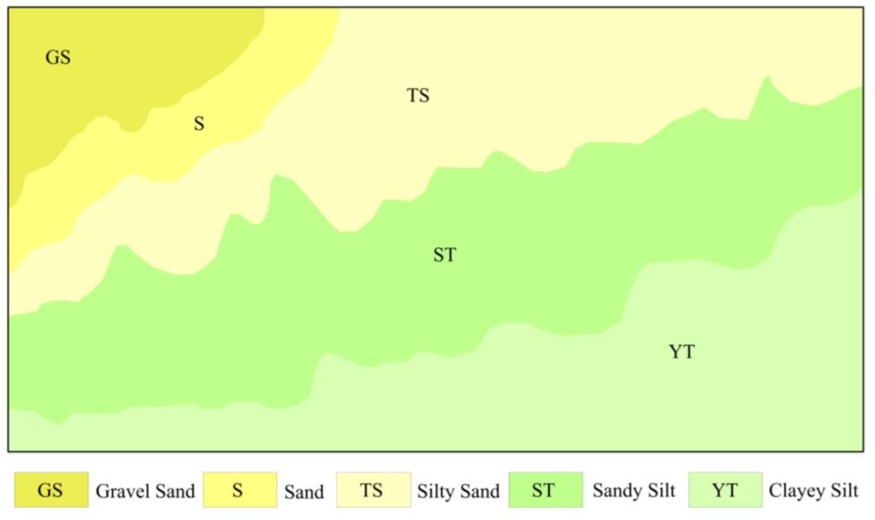
3.2. K-Means Cluster Analysis

The K-mean sediment classification method utilizes the cluster number K to classify marine sediment based on sampling results. This value represents a priori information and plays a crucial role in the accuracy of the classification. Selecting a value that is too small may result in the inability to differentiate between different types of marine sediments. Conversely, selecting a value that is too large may lead to inaccurate classification. To address this issue, this paper introduces two principles for determining an appropriate value for K in the classification of marine sediments.

• The classification principle of first-class groups in the Φ standard grain size classification table:The Udden–Wentworth isometric grain size classification standard (hereinafter referred to as the “Φ Size Standard”) is currently the most widely used grain size classification standard for sediments [42]. The Φ particle size standard divides the seafloor into five types: rock, gravel, sand, silt, and clay. Based on these five types, the seafloor is further classified into subcategories, such as pebbled muddy sand, silty sand, muddy silt, silty mud, and so on. To determine the value of the classification number K, the number of class groups belonging to the seafloor sampling point type in the Φ standard classification table of particle size is first determined, and its value is set as the K value.
• The principle of regional variation of marine sediment type:

The classification of marine sediment types based on the standard grain size classification table is a crucial step in understanding the characteristics of these sediments. However, it is important to consider the regional variation of marine sediment types and whether a finer classification can be carried out. This can be determined through assessing the value of K of the cluster type. The regional effect of the classification results of marine sediment is influenced by various factors, including marine sediment genesis and hydrodynamics. The type of marine sediment is expected to exhibit regional and continuous changes. Due to the correlation of these factors, there is often a certain degree of transition between marine sediment types. Increasing the value of K can improve the regional effect of marine sediment classification results, indicating that the classification results are effective. Conversely, if the regional effect is not good, it suggests that the addition of classification is not appropriate. Therefore, it is important to consider the regional variation of marine sediment types when classifying them based on the standard grain size classification table.

In the study area, the marine sediments can be classified into five types, namely gravelly sand, sand, silty sand, sandy silt, and mud. The classification presented above is derived from the Folk classification system, which was proposed by Folk et al. in 1970 [43]. This system utilizes two triangular diagrams, namely the gravel-bearing sediment classification triangular diagram and the gravel-free sediment classification triangular diagram. The gravel-bearing classification, as defined by Folk, comprises three distinct end-members: gravel, sand, and mud (in this context, mud refers to the combination of silt and clay). Through considering various gravel contents and sand–mud ratios, the lithic sediment can be further categorized into 14 different types. On the other hand, the gravel-free classification, an extension of the gravel-bearing triangular diagram, incorporates sand, silt, and clay as the three end-members. It classifies gravel-free sediments into 10 types based on different sand content and silt–clay ratio.

Applying the nomenclature principle and in conjunction with the Φ standard grain size classification chart [44], we have depicted the schematic representation of the sediment subcategory in the surveyed region (refer to Figure 9).

Based on Figure 9, it is evident that the sediment contains a relatively low amount of clay compared to sandy silt and clayey silt, and the similarity between the latter two is remarkably high. Furthermore, the sediment contains a relatively low amount of silt compared to sand and silty sand, and the similarity between the two is the second highest. In the classification of marine sediment, the higher the similarity between sediment types, the more challenging it becomes to differentiate them. Analyzing the similarity of sediment types in the test area can aid in accurately selecting the classification of marine sediment and evaluating the ability of marine sediment classification. For instance, it can help determine whether sediment types with high similarity, such as sand and silty sand, can be automatically distinguished.

Cluster analysis is a method of grouping similar objects together while ensuring that different groups have the greatest dissimilarity. The process of cluster analysis relies on measuring the similarity between target data. In this study, the three-dimensional points of the unit normal vector of all structural planes were projected onto the projection plane using the equal-area method. The similarity between two points, (x₁, y₁) and (x₂, y₂), was measured using the Euclidean distance d, where a smaller distance indicates a higher degree of similarity between the structural planes. The formula for Euclidean distance is given by Equation (6):

$$d^2={(x_1-x_2)}^2+{(y_1-y_2)}^2$$

(6)

When recalculating the clustering center of the dataset, the arithmetic mean value of the three-dimensional points representing the structural plane cannot be used to represent the clustering center. However, when using the equal-area projection, all points are on the plane, so it is reasonable to use the arithmetic mean value when updating the sample center of the clustering process. The formula for calculating the sample center is given by Equation (7):

$$\left\{\begin{array}{c}\overline{x}=\frac{1}{n}{\sum }_1^{n}x\\ \overline{y}=\frac{1}{n}{\sum }_1^{n}y\end{array}\right.$$

(7)

Here, n represents the number of all sample sets in the K cluster. Further K-Means clustering analysis was conducted on the classification results of the U-Net network to obtain classification results with a clear boundary of sediment type, as shown in Figure 10.

4. Discussion

4.1. Benefits of Improved U-Net Method for Predicting Mean Grain Size

In this study, we compared the performance of the improved U-Net method for predicting average particle size with the standard U-Net network, while keeping the training and test sets constant. To evaluate the refining effect of the improved U-Net on the prediction results, we conducted a qualitative comparison through examining the local details of the results. Figure 11 illustrates the comparison of the extraction results obtained from the two network models.

Upon comparison, it has been observed that the standard U-Net model gradually diminishes the low-dimensional features of the image. However, the improved U-Net model preserves the details of low-dimensional features at each coding layer and integrates them with the abstract information of the corresponding higher-dimensional features. This integration enhances the edge refinement effect of the base type, resulting in a more refined prediction output compared to the standard U-Net model.

To demonstrate the classification effectiveness of the improved U-Net and standard U-Net models, we have employed IoU and F1-Score metrics to evaluate the particle size prediction results of these two network models. IoU score is a widely accepted performance measure for object category segmentation, which represents the ratio of intersection and union between the truth set A and segmented result set B.

$$IoU=\frac{|A\cap B|}{|A\cup B|}$$

(8)

The F1-Score is a metric used to evaluate the effectiveness of image segmentation through taking into account both precision and recall, namely:

$$\left\{\begin{array}{c}Precision=\frac{TP}{TP+FP}\\ Recall=\frac{TP}{TP+FN}\\ F1-Score=2\times \frac{Precision\times Recall}{Precision+Recall}\end{array}\right.$$

(9)

where TP is the real value, i.e., A∩B; FP is true negative, namely B-(A∩B); FN is a false negative value, namely A-(A∩B).

The value range of IoU and F1-Score is [0, 1]. The closer the result is to 1, the more accurate the prediction result of the mean particle size of the seafloor is. The quantitative evaluation of the prediction results of average particle size is shown in

Table 2. Quantitative evaluation of sub-bottom sediment classification.

IoU (%)		F1-Score (%)
U-Net	Improved U-Net	U-Net	Improved U-Net
83.2	88.1	91.7	94.5

.

The findings presented in Table 2 demonstrate that the improved U-Net network yields superior average particle size prediction results. Specifically, the base classification results for the two indices increased by 4.9% and 2.8%, respectively, when compared to the standard U-Net network results. These results indicate that the improved U-Net model can enhance the accuracy of average particle size prediction in the study area.

4.2. Comparison of Sediment Classification Results

The study area is situated in the outer margin of the ancient Pearl River Delta [45,46]. The surface sediment is distributed in a NE–SW zonal direction parallel to the coast, with the grain size gradually decreasing with increasing water depth [47]. The coastline has receded to the slope area with a depth of over 100 m, leading to the continuous erosion of the shelf slope break of the northern South China Sea and the deposition of new terrigenous materials. The shelf and slope area have developed many buried ancient channels, coastal dunes, seafloor dunes, and underwater deltas [48].

In this area, there are two genetic types of marine sediments, as identified by Qin Yunshan in 1963 [49]. One type consists of modern fine-grained debris transported by rivers, while the other type consists of residual deposits from the low glacial sea level of the early late Pleistocene. The sediment particle components in this area exhibit characteristics of the interleaved deposition of coarse and fine grains, influenced by the characteristics of the sediments in the source area and subsequent transformations. The coarse-grained materials, which have a high content, are primarily the result of long-term deposition in a high-energy environment. During the post-glacial sea level rise, these coarse-grained materials may have been covered by fine-grained sediments [50].

The northern continental slope of the South China Sea exhibits distinct zonal distribution characteristics of sediments. A detailed description of the sedimentary types in the South China Sea was compiled through analyzing surface sediment sampling data by Shi et al., 2022 [51], as shown in Figure 12. In the shallow-water area, the sediments mainly consist of gravel sand, with a higher proportion of gravel and ancient coral reef debris. The mean grain size is relatively coarse, suggesting that beach sand or shallow sea sand from the period of low sea level has been selectively retained by modern hydrodynamic conditions. Near the slope break of the middle and upper shelf, the bottom material is primarily sand, with most sediments being relatively fine and well-sorted. It is speculated that these sediments may be a mixture of river input from the ancient Pearl River and materials from the low sea level period.

In the deep-water area with a water depth greater than 1000 m, the sediments are predominantly fine-grained silty sand, sandy silt, and clay silt [34,52]. In the middle submarine canyon area, the sediments consist mainly of mixed components of sand and silt, with medium sorting. It is speculated that the beach sand from the low sea level period was mixed with terrigenous clastic sediments brought by the ancient Pearl River and may also contain some turbidite sediments. The sediment particles in the head area of the canyon are coarser and mainly silty sand, likely due to the influence of the hydrodynamic environment. In the middle of the canyon, the sediments are primarily silty sand. In the lower part of the study area, located in the deep-water area, the sediments are dominated by clayey silt with a smaller particle size compared to other sedimentary areas. These sediments are presumed to be the result of ancient Pearl River input material in a late low hydrodynamic environment.

Based on the above analysis, the sediment classification results obtained using this method are consistent with the sedimentary environment characteristics of the study area. Furthermore, they show a high level of agreement with the sediment type map of the South China Sea, providing further evidence for the reliability of the sediment classification results.

5. Conclusions

In this study, we conducted a comprehensive analysis and research on the classification and characteristics of marine sediment types in the northern continental slope of the South China Sea, based on data of water depth, slope, reflection intensity, and sampling tests. Our findings are as follows:

(1)

We developed a sediment classification method based on an improved U-Net network and K-means clustering analysis. This method allowed us to classify five sediment types, including gravelly sand, sand, silty sand, sandy silt, and clayey silt, in the study area.

(2)

In this study, we compared the results obtained from an improved U-Net model with those of a standard U-Net model for mean grain size prediction. It was found that the improved U-Net model outperformed the standard U-Net model in terms of IoU and F1-Score, with improvements of 4.9% and 2.8%, respectively, in the two metrics for mean grain size prediction. This indicates that the improved U-Net model can improve the accuracy of mean grain size prediction in the study area.

(3)

An optimized K-means clustering algorithm was employed to conduct sediment type classification, improving the effectiveness of edge extraction for sediment types and enhancing the accuracy of sediment type classification. A comparison with the sediment type map of the South China Sea demonstrated a high level of consistency, further validating the applicability of this method in sediment classification.

References

- Hamilton, L.; Mulhearn, P.; Poeckert, R. Comparison of RoxAnn and QTC-View acoustic bottom classification system performance for the Cairns area, Great Barrier Reef, Australia. Cont. Shelf Res. 1999, 19, 1577–1597. [Google Scholar] [CrossRef]
- Preston, J.M.; Collins, W.T.; Mosher, D.C.; Poeckert, R.H.; Kuwahara, R.H. The strength of correlations between geotechnical variables and acoustic classifications. In Proceedings of the Oceans ‘99. MTS/IEEE. Riding the Crest into the 21st Century. Conference and Exhibition. Conference Proceedings (IEEE Cat. No.99CH37008), Seattle, WA, USA, 13–16 September 1999; pp. 1123–1128. [Google Scholar]
- Tęgowski, J.; Łubniewski, Z. The use of fractal properties of echo signals for acoustical classification of bottom sediments. Acta Acust. United Acust. 2000, 86, 276–282. [Google Scholar]
- Preston, J.M. Shallow-water bottom classification: High speed echo-sampling captures detail for precise sediment classification. Hydro Int. 2001, 5, 30–33. [Google Scholar]
- Preston, J.M.; Christney, A.C.; Bloomer, S.F.; Beaudet, I.L. Seabed classification of multibeam sonar image. In Proceedings of the MTS/IEEE Oceans 2001. An Ocean Odyssey. Conference Proceedings (IEEE Cat. No.01CH37295), Honolulu, HI, USA, 5–8 November 2001; Volume 4, pp. 2616–2623. [Google Scholar]
- Giovanni, D.F.; Renato, T.; Gabriella, D.M.; Sara, I.; Simone, S.; Iain, M.P. Relationships between multibeam backscatter, sediment grain size and Posidonia oceanica seagrass distribution. Cont. Shelf Res. 2010, 30, 1941–1950. [Google Scholar]
- Wienberg, C.; Wintersteller, P.; Beuck, L.; Hebbeln, D. Coral Patch seamount (NE Atlantic) a sedimentological and megafaunal reconnaissance based on video and hydroacoustic surveys. Biogeosciences 2013, 10, 3421–3443. [Google Scholar] [CrossRef]
- Mcgee, T.M. The use of marine seismic profiling for environmental assessment. Geophys. Prospect. 1990, 38, 861–880. [Google Scholar] [CrossRef]
- Wu, Z.Y.; Zheng, Y.L.; Chu, F.Y.; Tao, C.H.; Gao, J.Y. Research Status and Prospect of Sonar Detecting Techniques Near Submarine. Adv. Earth Sci. 2005, 20, 1210–1217. [Google Scholar]
- Li, X.; Liu, B.; Liu, L.; Zheng, J.; Zhou, S.; Zhou, Q. Prediction for potential landslide zones using seismic amplitude in Liwan gas field, northern South China Sea. J. Ocean. Univ. China 2017, 16, 1035–1042. [Google Scholar] [CrossRef]
- Dong, Y.K.; Wang, D.; Randolph, M. Investigation of impact forces on pipeline by submarine landslide with material point method. Ocean. Eng. 2017, 146, 21–28. [Google Scholar] [CrossRef]
- Tao, C.; Jin, X.; Xu, F.; Gu, C.; He, Y. Current Status and Prospects of Research on Acoustic Seabed Sediment Classification Technologies. East China Sea 2004, 22, 28–33. [Google Scholar]
- Dong, Y.K.; Liao, Z.X.; Liu, Q.B.; Cui, L. Potential failure patterns of a large landslide complex in the Three Gorges Reservoir area. Bull. Eng. Geol. Environ. 2023, 82, 41. [Google Scholar] [CrossRef]
- Kim, G.; Kim, D.C.; Park, S.C.; Lee, G.H. Chirp (2–7 kHz) echo characters and geotechnical properties of surface sediments in the Ulleung Basin, the East Sea. J. Geosci. 1999, 3, 213–224. [Google Scholar] [CrossRef]
- Schock, S.G. A method for estimating the physical and acoustic properties of the sea bed using chirp sonar data. IEEE J. Ocean. Eng. 2004, 29, 1200–1217. [Google Scholar] [CrossRef]
- Schock, S.G. Remote estimates of physical and acoustic sediment properties in the South China Sea using chirp sonar data and the biot model. IEEE J. Ocean. Eng. 2004, 29, 1218–1230. [Google Scholar] [CrossRef]
- Vardy, M.E. Deriving shallow-water sediment properties using post-stack acoustic impedance inversion. Near Surf. Geophys. 2015, 13, 143–154. [Google Scholar] [CrossRef]
- Zhang, Z.M.; Huo, H.; Zhao, F.Y. Survey of object detection algorithm based on deep convolutional neural networks. J. Chin. Mini-Micro Comput. Syst. 2019, 40, 1825–1831. [Google Scholar]
- Parkhi, O.M.; Vedaldi, A.; Zisserman, A. Deep face recognition. In Proceedings of the British Machine Vision Conference, Swansea, UK, 7–10 September 2016. [Google Scholar]
- Dong, Y.K.; Cui, L.; Zhang, X. Multiple-GPU for three dimensional MPM based on single-root complex. Int. J. Numer. Methods Eng. 2022, 123, 1481–1504. [Google Scholar] [CrossRef]
- Berthold, T.; Leichter, A.; Rosenhahn, B.; Berkhahn, V.; Valerius, J. Seabed sediment classification of side-scan sonar data using convolutional neural networks. In Proceedings of the 2017 IEEE Symposium Series on Computational Intelligence (SSCI), Honolulu, HI, USA, 8 February 2018. [Google Scholar]
- Luo, X.; Qin, X.; Wu, Z.; Yang, F.; Wang, M.; Shang, J. Sediment classification of small-size seabed acoustic images using convolutional neural networks. IEEE Access 2019, 7, 98331–98339. [Google Scholar] [CrossRef]
- Wang, H.; Zhou, Q.; Wei, S.; Xue, X.; Zhou, X.; Zhang, X. Research on Seabed Sediment Classification Based on the MSC-Transformer and Sub-Bottom Profiler. J. Mar. Sci. Eng. 2023, 11, 1074. [Google Scholar] [CrossRef]
- Tegowski, J. Acoustical classification of the bottom sediments in the southern Baltic Sea. Quat. Int. 2005, 130, 153–161. [Google Scholar] [CrossRef]
- Lu, L.; Jin, S.; Bian, G.; Cui, Y.; Xia, W. The application of K-means clustering analysis algorithm in multibeam seafloor classification. Hydrogr. Surv. Charting 2018, 38, 64–68. [Google Scholar]
- Ronneberger, O.; Fischer, P.; Brox, T. U-Net: Convolutional Networks for Biomedical Image Segmentation. In International Conference on Medical Image Computing and Computer Assisted Intervention; Springer: Munich, Germany, 2015; pp. 234–241. [Google Scholar]
- Maayan, F.A.; Avi, B.C.; Rula, A.; Hayit, G. Improving the Segmentation of Anatomical Structures in Chest Radiographs Using U-Net with an ImageNet Pre-trained Encoder. Image Anal. Mov. Organ Breast Thorac. Images 2018, 11040, 159–168. [Google Scholar]
- Iglovikov, V.; Shvets, A. TernausNet: U-Net with VGG11 Encoder Pre-Trained on ImageNet for Image Segmentation. arXiv 2018, arXiv:1801.05746. [Google Scholar]
- Ward, J.H. Hierarchical Grouping to Optimize an Objective Function. J. Am. Stat. Assoc. 1963, 58, 236–244. [Google Scholar] [CrossRef]
- Kaski, S.; Kangas, J.; Kohonen, T. Bibliography of self-organizing map (SOM) papers: 1981–1997. Neural Comput. Surv. 2002, 1, 1–156. [Google Scholar]
- Frey, B.J.; Dueck, D. Clustering by passing messages between data points. Science 2007, 315, 972–976. [Google Scholar] [CrossRef]
- Zhu, L.; Fu, M.; Liu, L.; Li, J.; Gao, S. Canyon morphology and sediments on northern slope of the Baiyun Sag. Mar. Geol. Quat. Geol. 2014, 34, 1–9. [Google Scholar]
- Zhou, Q.; Li, X.; Xu, Y.; Liu, L. A rapid method to recognize submarine landslides based on the principle of water depth gradient: A case of Baiyun deep-water area, north slope of the South China Sea. Acta Oceanol. Sin. 2017, 39, 138–147. [Google Scholar]
- Li, A.; Li, Y.; Le, G. Origin of tellurium anomalies in deep-sea sediments. Acta Geosci. Sin. 2005, 26, 186–189. [Google Scholar]
- Zhu, C.; Zhou, L.; Zhang, H.; Sheng, C. Preliminary study of physical and mechanical properties of surface sediment in Northern South China Sea. J. Eng. Geol. 2017, 25, 1566–1573. [Google Scholar]
- Vijay, B.; Alex, K.; Roberto, C. SegNet: A Deep Convolutional Encoder-decoder Architecture for Image Segmentation. IEEE Trans. Pattern Anal. Mach. Intell. 2017, 39, 2481–2495. [Google Scholar]
- Li, Y.; Wang, Q.; Chen, J.; Xu, L. K-means algorithm based on particle swarm optimization for the identification of rock discontinuity sets. Rock Mech. Rock Eng. 2015, 48, 375–385. [Google Scholar] [CrossRef]
- Krizhevsky, A.; Sutskever, I.; Hinton, G.E. ImageNet Classification with Deep Convolutional Neural Networks. Adv. Neural Inf. Process. Syst. 2012, 25, 1097–1105. [Google Scholar] [CrossRef]
- Kumar, P.; Nagar, P.; Arora, C.; Gupta, A. U-SegNet: Fully Convolutional Neural Network based automatic Brain tissue segmentation Tool. arXiv 2018, arXiv:1806.04429. [Google Scholar]
- Ketkar, N. Stochastic Gradient Descent. In Deep Learning with Python; Apress: Berkeley, CA, USA, 2017; pp. 113–132. [Google Scholar]
- Long, J.; Shelhamer, E.; Darrell, T. Fully Convolutional Networks for Semantic Segmentation. In Proceedings of the IEEE Conference on Computer Vision and Pattern Recognition, Boston, MA, USA, 7–12 June 2015; IEEE Computer Society: Washington, DC, USA, 2015; pp. 3431–3440. [Google Scholar]
- Terry, J.P.; Goff, J. Megaclasts: Proposed Revised Nomenclature at the Coarse End of the Udden-Wentworth Grain-Size Scale for Sedimentary Particles. J. Sediment. Res. 2014, 84, 192–197. [Google Scholar] [CrossRef]
- Folk, R.L.; Andrews, P.B.; Lewis, D.W. Detrital sedimentary rock classification and nomenclature for use in New Zealand. New Zealand J. Geol. Geophys. 1970, 13, 937–968. [Google Scholar] [CrossRef]
- Blair, T.C.; Mcpherson, J.G. Grain-size and textural classification of coarse sedimentary particles. J. Sediment. Res. 1999, 69, 6–19. [Google Scholar] [CrossRef]
- Rahman, M.A.; Wang, Y. Optimizing Intersection-Over-Union in Deep Neural Networks for Image Segmentation. In International Symposium on Visual Computing; Springer International Publishing: Las Vegas, Nevada, 2016; pp. 234–244. [Google Scholar]
- Lever, J.; Krzywinski, M.; Altman, N. Points of singnificance: Classification evaluation. Nat. Methods 2016, 13, 603–604. [Google Scholar] [CrossRef]
- Bao, C. Buride ancient channels and deltas in the Zhujiang River mouth shelf area. Mar. Geol. Quat. Geol. 1995, 15, 25–36. [Google Scholar]
- Yang, T.; Xue, Z.; Yang, J.; Jiang, S. Characteristics of hydrogen and oxygen isotopic composition of pore water in Marine sediments in the northern part of the south China sea. Acta Geosci. Sin. 2003, 24, 511–514. [Google Scholar]
- Qin, Y. A preliminary study on the topography and sedimentary types of continental shelf seas in China. Oceanol. Et Limnol. Sin. 1963, 71–85. [Google Scholar]
- Lu, B. Study on sediments and their physical properties in the waters of Dongsha Islands. Acta Oceanol. Sin. 1996, 18, 82–89. [Google Scholar]
- Shi, X.; Liu, S.; Qiao, S.; Liu, Y.; Wang, K. Sediment Type Map of the South China Sea; Science Press: Beijing, China, 2022. [Google Scholar]
- Liu, J.; Xiang, R.; Chen, Z.; Chen, M.; Yan, W.; Zhang, L.; Chen, H. Sources, transport and deposition of surface sediments from the South China Sea. Deep. Sea Res. Part I Oceanogr. Res. Pap. 2013, 71, 92–102. [Google Scholar] [CrossRef]