

Scattering Properties of Non-Gaussian Ocean Surface with the SSA Model Applied to GNSS-R

Abstract
1. Introduction
2. Materials and Methods
2.1. Data
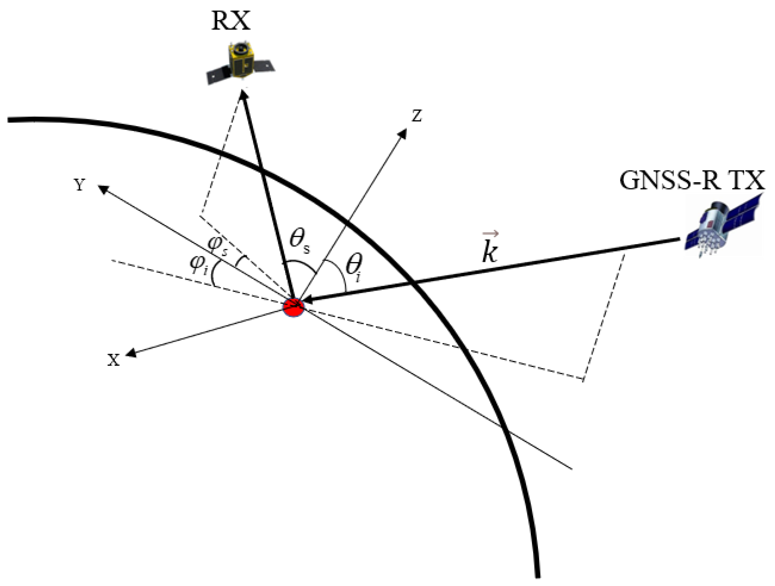
2.2. Geometry
2.3. Polarization Synthesis
3. Scattering of Non-Gaussian Ocean Surface
3.1. Scattering Model
3.2. Derivation of Non-Gaussian Statistics
3.3. L-Band Forward Scattering Coefficient
4. Results
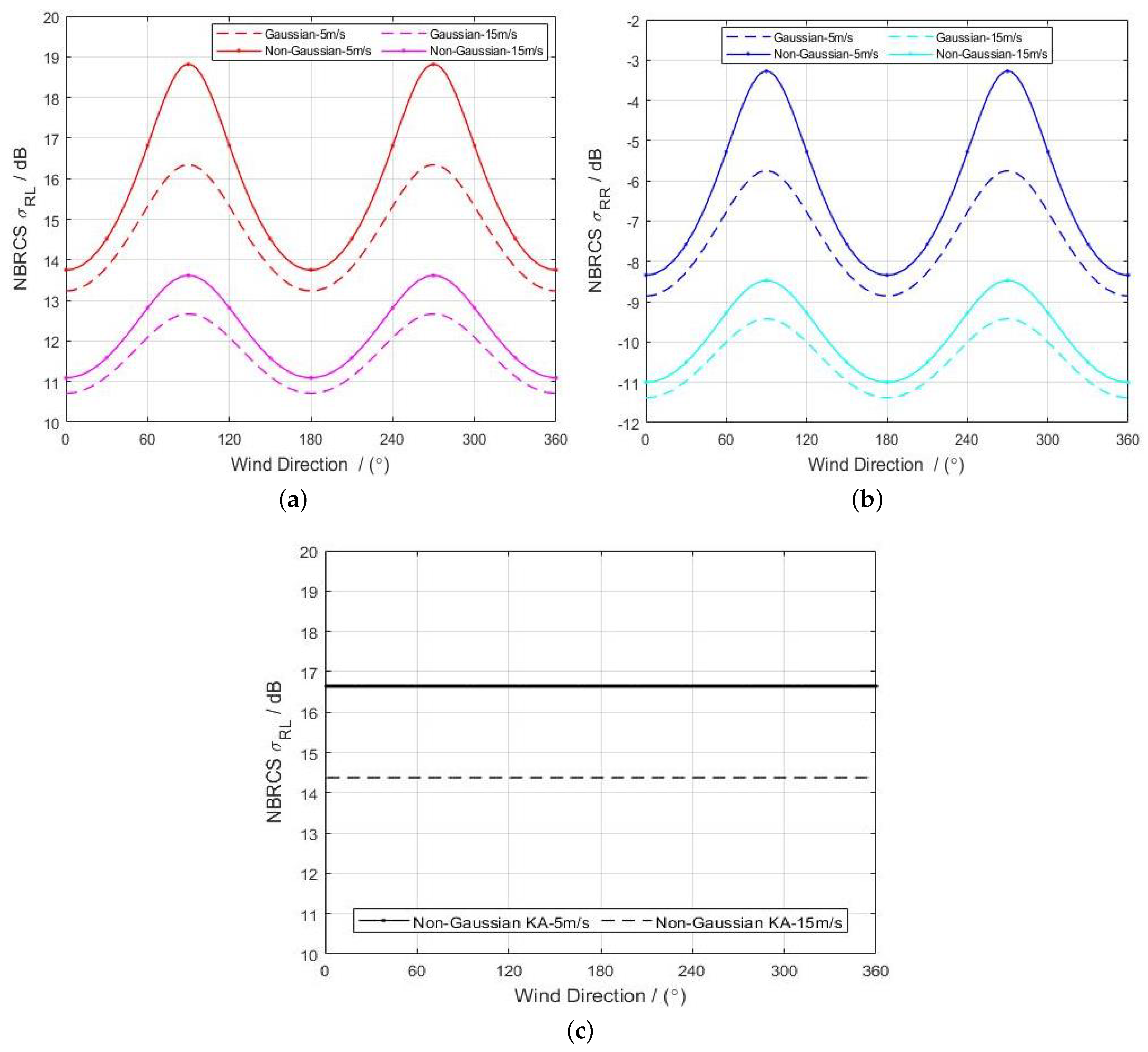
4.1. The Effect of Observation Angle on BRCS
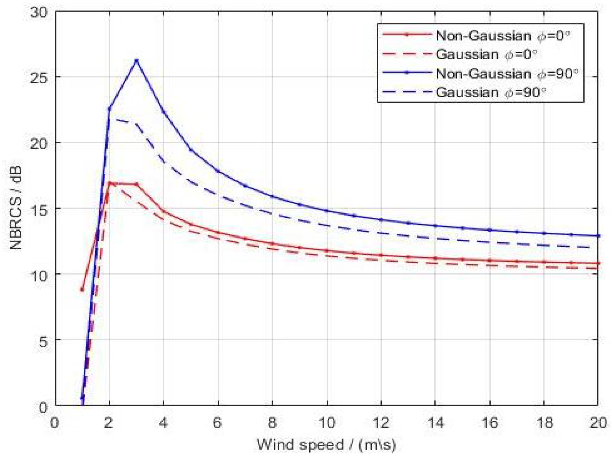
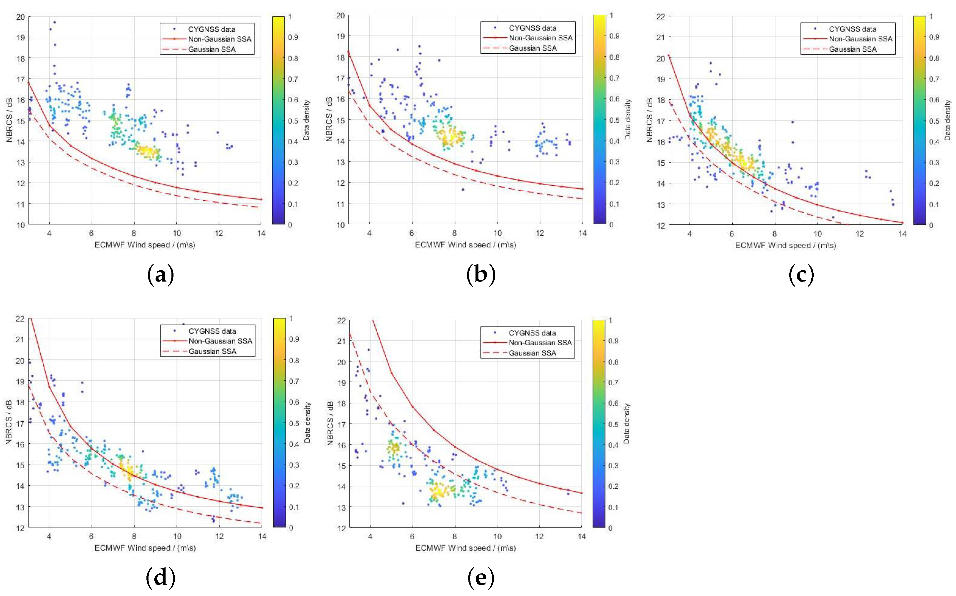
4.2. The Effect of Ocean Wind on NBRCS
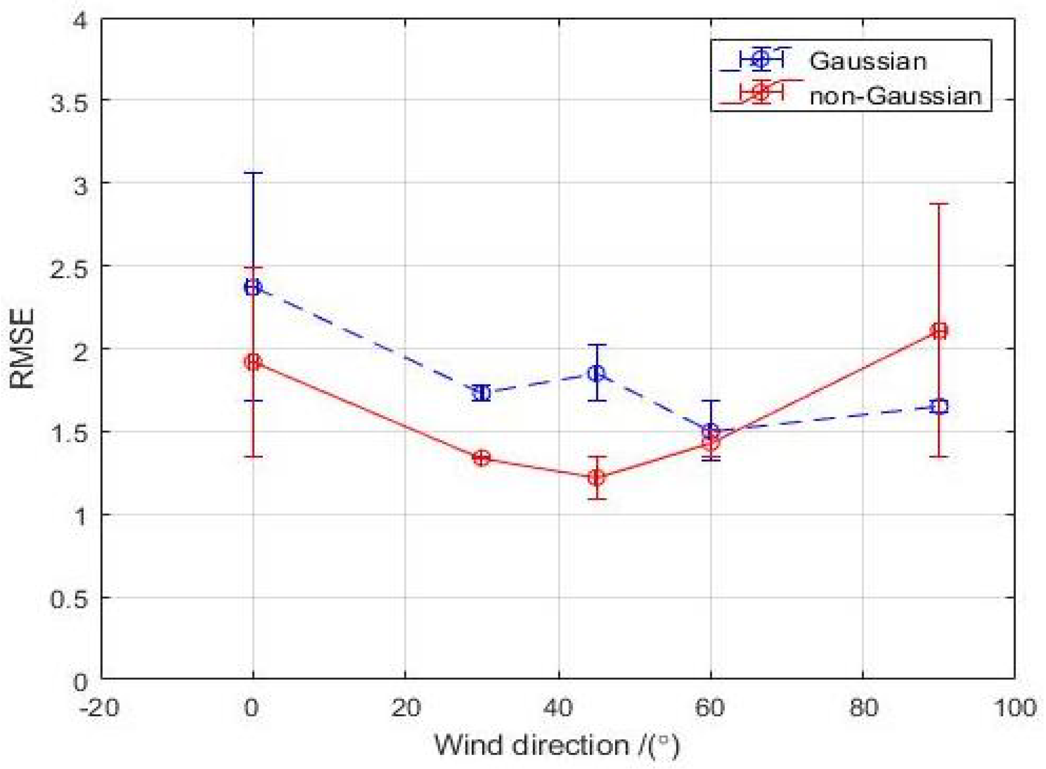
5. Discussion
6. Conclusions
Author Contributions
Funding
Data Availability Statement
Acknowledgments
Conflicts of Interest
References
- Gleason, S. Space-based GNSS scatterometry: Ocean wind sensing using an empirically calibrated model. IEEE Trans. Geosci. Remote Sens. 2013, 51, 4853–4863. [Google Scholar] [CrossRef]
- Clarizia, M.P.; Ruf, C.S. Wind speed retrieval algorithm for the Cyclone Global Navigation Satellite System (CYGNSS) mission. IEEE Trans. Geosci. Remote Sens. 2016, 54, 4419–4432. [Google Scholar] [CrossRef]
- Ruf, C.S.; Balasubramaniam, R. Development of the CYGNSS geophysical model function for wind speed. IEEE J. Sel. Top. Appl. Earth Obs. Remote Sens. 2018, 12, 66–77. [Google Scholar] [CrossRef]
- Clarizia, M.P.; Ruf, C.S. Statistical derivation of wind speeds from CYGNSS data. IEEE Trans. Geosci. Remote Sens. 2020, 58, 3955–3964. [Google Scholar] [CrossRef]
- Guo, W.; Du, H.; Cheong, J.W.; Southwell, B.J.; Dempster, A.G. GNSS-R wind speed retrieval of sea surface based on particle swarm optimization algorithm. IEEE Trans. Geosci. Remote Sens. 2021, 60, 4202414. [Google Scholar] [CrossRef]
- Cardellach, E.; Rius, A. A new technique to sense non-Gaussian features of the sea surface from L-band bi-static GNSS reflections. Remote Sens. Environ. 2008, 112, 2927–2937. [Google Scholar] [CrossRef]
- Valencia, E.; Zavorotny, V.U.; Akos, D.M.; Camps, A. Using DDM asymmetry metrics for wind direction retrieval from GPS ocean-scattered signals in airborne experiments. IEEE Trans. Geosci. Remote Sens. 2013, 52, 3924–3936. [Google Scholar] [CrossRef]
- Guan, D.; Park, H.; Camps, A.; Wang, Y.; Onrubia, R.; Querol, J.; Pascual, D. Wind direction signatures in GNSS-R observables from space. Remote Sens. 2018, 10, 198. [Google Scholar] [CrossRef]
- Zhang, G.; Yang, D.; Yu, Y.; Wang, F. Wind direction retrieval using spaceborne GNSS-R in nonspecular geometry. IEEE J. Sel. Top. Appl. Earth Obs. Remote Sens. 2020, 13, 649–658. [Google Scholar] [CrossRef]
- Pascual, D.; Clarizia, M.P.; Ruf, C.S. Spaceborne Demonstration of GNSS-R scattering cross section sensitivity to wind direction. IEEE Geosci. Remote Sens. Lett. 2021, 19, 8006005. [Google Scholar] [CrossRef]
- Li, C.; Huang, W. Sea surface oil slick detection from GNSS-R Delay-Doppler Maps using the spatial integration approach. In Proceedings of the 2013 IEEE Radar Conference (RadarCon13), Ottawa, ON, Canada, 29 April–3 May 2013; pp. 1–6. [Google Scholar]
- Li, C.; Huang, W.; Gleason, S. Dual antenna space-based GNSS-R ocean surface mapping: Oil slick and tropical cyclone sensing. IEEE J. Sel. Top. Appl. Earth Obs. Remote Sens. 2014, 8, 425–435. [Google Scholar] [CrossRef]
- Zhang, Y.; Chen, S.; Hong, Z.; Han, Y.; Li, B.; Yang, S.; Wang, J. Feasibility of oil slick detection using BeiDou-R coastal simulation. Math. Probl. Eng. 2017, 2017, 8098029. [Google Scholar] [CrossRef]
- Clarizia, M.P.; Ruf, C.; Cipollini, P.; Zuffada, C. First spaceborne observation of sea surface height using GPS-Reflectometry. Geophys. Res. Lett. 2016, 43, 767–774. [Google Scholar] [CrossRef]
- Cardellach, E.; Li, W.; Rius, A.; Semmling, M.; Wickert, J.; Zus, F.; Ruf, C.S.; Buontempo, C. First precise spaceborne sea surface altimetry with GNSS reflected signals. IEEE J. Sel. Top. Appl. Earth Obs. Remote Sens. 2019, 13, 102–112. [Google Scholar] [CrossRef]
- Alonso-Arroyo, A.; Zavorotny, V.U.; Camps, A. Sea ice detection using UK TDS-1 GNSS-R data. IEEE Trans. Geosci. Remote Sens. 2017, 55, 4989–5001. [Google Scholar] [CrossRef]
- Rodriguez-Alvarez, N.; Holt, B.; Jaruwatanadilok, S.; Podest, E.; Cavanaugh, K.C. An Arctic sea ice multi-step classification based on GNSS-R data from the TDS-1 mission. Remote Sens. Environ. 2019, 230, 111202. [Google Scholar] [CrossRef]
- Li, W.; Cardellach, E.; Fabra, F.; Rius, A.; Ribó, S.; Martín-Neira, M. First spaceborne phase altimetry over sea ice using TechDemoSat-1 GNSS-R signals. Geophys. Res. Lett. 2017, 44, 8369–8376. [Google Scholar] [CrossRef]
- Mayers, D.; Ruf, C. Measuring ice thickness with CYGNSS altimetry. In Proceedings of the IGARSS 2018—2018 IEEE International Geoscience and Remote Sensing Symposium, Valencia, Spain, 22–27 July 2018; pp. 8535–8538. [Google Scholar]
- Unwin, M.; Jales, P.; Tye, J.; Gommenginger, C.; Foti, G.; Rosello, J. Spaceborne GNSS-reflectometry on TechDemoSat-1: Early mission operations and exploitation. IEEE J. Sel. Top. Appl. Earth Obs. Remote Sens. 2016, 9, 4525–4539. [Google Scholar] [CrossRef]
- Ruf, C.; Chang, P.S.; Clarizia, M.-P.; Gleason, S.; Jelenak, Z.; Majumdar, S.; Morris, M.; Murray, J.; Musko, S.; Posselt, D.; et al. CYGNSS Handbook; Michigan Publishing Services: Ann Arbor, MI, USA, 2022. [Google Scholar]
- Yang, G.; Bai, W.; Wang, J.; Hu, X.; Zhang, P.; Sun, Y.; Xu, N.; Zhai, X.; Xiao, X.; Xia, J.; et al. FY3E GNOS II GNSS reflectometry: Mission review and first results. Remote Sens. 2022, 14, 988. [Google Scholar] [CrossRef]
- Foti, G.; Gommenginger, C.; Jales, P.; Unwin, M.; Shaw, A.; Robertson, C.; Rosello, J. Spaceborne GNSS reflectometry for ocean winds: First results from the UK TechDemoSat-1 mission. Geophys. Res. Lett. 2015, 42, 5435–5441. [Google Scholar] [CrossRef]
- Zavorotny, V.U.; Voronovich, A.G. Scattering of GPS signals from the ocean with wind remote sensing application. IEEE Trans. Geosci. Remote Sens. 2000, 38, 951–964. [Google Scholar] [CrossRef]
- Zuffada, C.; Elfouhaily, T.; Lowe, S. Sensitivity analysis of wind vector measurements from ocean reflected GPS signals. Remote Sens. Environ. 2003, 88, 341–350. [Google Scholar] [CrossRef]
- Li, C.; Huang, W. An algorithm for sea-surface wind field retrieval from GNSS-R delay-Doppler map. IEEE Geosci. Remote Sens. Lett. 2014, 11, 2110–2114. [Google Scholar]
- Zavorotny, V.U.; Voronovich, A.G. Recent progress on forward scattering modeling for GNSS reflectometry. In Proceedings of the 2014 IEEE Geoscience and Remote Sensing Symposium, Quebec City, QC, Canada, 13–18 July 2014; pp. 3814–3817. [Google Scholar]
- Munoz-Martin, J.F.; Rodriguez-Alvarez, N.; Bosch-Lluis, X.; Oudrhiri, K. Stokes parameters retrieval and calibration of hybrid compact polarimetric GNSS-R signals. IEEE Trans. Geosci. Remote Sens. 2022, 60, 5113911. [Google Scholar] [CrossRef]
- Munoz-Martin, J.F.; Rodriguez-Alvarez, N.; Bosch-Lluis, X.; Oudrhiri, K. Detection Probability of Polarimetric GNSS-R Signals. IEEE Geosci. Remote Sens. Lett. 2023, 20, 3500905. [Google Scholar] [CrossRef]
- Zuffada, C.; Fung, A.; Parker, J.; Okolicanyi, M.; Huang, E. Polarization properties of the GPS signal scattered off a wind-driven ocean. IEEE Trans. Antennas Propag. 2004, 52, 172–188. [Google Scholar] [CrossRef]
- Clarizia, M.P.; Gommenginger, C.; Di Bisceglie, M.; Galdi, C.; Srokosz, M.A. Simulation of L-band bistatic returns from the ocean surface: A facet approach with application to ocean GNSS reflectometry. IEEE Trans. Geosci. Remote Sens. 2011, 50, 960–971. [Google Scholar] [CrossRef]
- Zavorotny, V.U.; Voronovich, A.G. Bistatic radar scattering from an ocean surface in the small-slope approximation. In Proceedings of the IEEE 1999 International Geoscience and Remote Sensing Symposium. IGARSS’99 (Cat. No. 99CH36293), Hamburg, Germany, 28 June–2 July 1999; Volume 5, pp. 2419–2421. [Google Scholar]
- Voronovich, A. Small-slope approximation for electromagnetic wave scattering at a rough interface of two dielectric half-spaces. Waves Random Media 1994, 4, 337. [Google Scholar] [CrossRef]
- Zavorotny, Z.; Voronovich, A.G.; Katzberg, S.J.; Garrison, J.L.; Komjathy, A. Extraction of sea state and wind speed from reflected GPS signals: Modeling and aircraft measurements. In Proceedings of the IGARSS 2000. IEEE 2000 International Geoscience and Remote Sensing Symposium. Taking the Pulse of the Planet: The Role of Remote Sensing in Managing the Environment. Proceedings (Cat. No. 00CH37120), Honolulu, HI, USA, 24–28 July 2000; Volume 4, pp. 1507–1509. [Google Scholar]
- Fung, A.; Tjuatja, S. Backscattering and emission signatures of randomly rough surfaces based on IEM. In Proceedings of the Proceedings of IGARSS’93—IEEE International Geoscience and Remote Sensing Symposium, Tokyo, Japan, 18–21 August 1993; pp. 1006–1008. [Google Scholar]
- Awada, A.; Khenchaf, A.; Coatanhay, A. Bistatic radar scattering from an ocean surface at L-band. In Proceedings of the 2006 IEEE Conference on Radar, Verona, NY, USA, 24–27 April 2006. [Google Scholar]
- Voronovich, A.G.; Zavorotny, V.U. Full-polarization modeling of monostatic and bistatic radar scattering from a rough sea surface. IEEE Trans. Antennas Propag. 2013, 62, 1362–1371. [Google Scholar] [CrossRef]
- Elfouhaily, T.; Chapron, B.; Katsaros, K.; Vandemark, D. A unified directional spectrum for long and short wind-driven waves. J. Geophys. Res. Ocean. 1997, 102, 15781–15796. [Google Scholar] [CrossRef]
- Beckmann, P. Scattering by non-Gaussian surfaces. IEEE Trans. Antennas Propag. 1973, 21, 169–175. [Google Scholar] [CrossRef]
- Cox, C. Statistics of the sea surface derived from sun glitter. J. Mar. Res. 1954, 13, 198–227. [Google Scholar]
- Longuet-Higgins, M.S. On the skewness of sea-surface slopes. J. Phys. Oceanogr. 1982, 12, 1283–1291. [Google Scholar] [CrossRef]
- Chapron, B.; Kerbaol, V.; Vandemark, D.; Elfouhaily, T. Importance of peakedness in sea surface slope measurements and applications. J. Geophys. Res. Ocean. 2000, 105, 17195–17202. [Google Scholar] [CrossRef]
- Nickolaev, N.; Yordanov, O.; Michalev, M. Non-Gaussian effects in the two-scale model for rough surface scattering. J. Geophys. Res. Ocean. 1992, 97, 15617–15624. [Google Scholar] [CrossRef]
- Chen, K.S.; Fung, A.K.; Weissman, D.A. A backscattering model for ocean surface. IEEE Trans. Geosci. Remote Sens. 1992, 30, 811–817. [Google Scholar] [CrossRef]
- Bourlier, C. Azimuthal harmonic coefficients of the microwave backscattering from a non-Gaussian ocean surface with the first-order SSA model. IEEE Trans. Geosci. Remote Sens. 2004, 42, 2600–2611. [Google Scholar] [CrossRef]
- Park, J.; Johnson, J.T. A study of wind direction effects on sea surface specular scattering for GNSS-R applications. IEEE J. Sel. Top. Appl. Earth Obs. Remote Sens. 2017, 10, 4677–4685. [Google Scholar] [CrossRef]
- Wang, S.; Shi, S.; Ni, B. Joint use of spaceborne microwave sensor data and CYGNSS data to observe tropical cyclones. Remote Sens. 2020, 12, 3124. [Google Scholar] [CrossRef]
- Cardellach, E.; Nan, Y.; Li, W.; Padullés, R.; Ribó, S.; Rius, A. Variational retrievals of high winds using uncalibrated CyGNSS observables. Remote Sens. 2020, 12, 3930. [Google Scholar] [CrossRef]
- Saïd, F.; Soisuvarn, S.; Jelenak, Z.; Chang, P.S. Performance assessment of simulated CYGNSS measurements in the tropical cyclone environment. IEEE J. Sel. Top. Appl. Earth Obs. Remote Sens. 2016, 9, 4709–4719. [Google Scholar] [CrossRef]
- Nord, M.E.; Ainsworth, T.L.; Lee, J.S.; Stacy, N.J. Comparison of compact polarimetric synthetic aperture radar modes. IEEE Trans. Geosci. Remote Sens. 2008, 47, 174–188. [Google Scholar] [CrossRef]
- Voronovich, A.; Zavorotny, V. Theoretical model for scattering of radar signals in K u-and C-bands from a rough sea surface with breaking waves. Waves Random Media 2001, 11, 247. [Google Scholar] [CrossRef]
- McDaniel, S.T. Small-slope predictions of microwave backscatter from the sea surface. Waves Random Media 2001, 11, 343. [Google Scholar] [CrossRef]
- Longuet-Higgins, M.S. The effect of non-linearities on statistical distributions in the theory of sea waves. J. Fluid Mech. 1963, 17, 459–480. [Google Scholar] [CrossRef]
- Thompson, D.R.; Elfouhaily, T.M.; Garrison, J.L. An improved geometrical optics model for bistatic GPS scattering from the ocean surface. IEEE Trans. Geosci. Remote Sens. 2005, 43, 2810–2821. [Google Scholar] [CrossRef]
- Jing, C.; Niu, X.; Duan, C.; Lu, F.; Di, G.; Yang, X. Sea surface wind speed retrieval from the first Chinese GNSS-R mission: Technique and preliminary results. Remote Sens. 2019, 11, 3013. [Google Scholar] [CrossRef]
- Ruf, C.S.; Gleason, S.; McKague, D.S. Assessment of CYGNSS wind speed retrieval uncertainty. IEEE J. Sel. Top. Appl. Earth Obs. Remote Sens. 2018, 12, 87–97. [Google Scholar] [CrossRef]
- Wang, F.; Yang, D.; Yang, L. Feasibility of wind direction observation using low-altitude global navigation satellite system-reflectometry. IEEE J. Sel. Top. Appl. Earth Obs. Remote Sens. 2018, 11, 5063–5075. [Google Scholar] [CrossRef]
- Gleason, S.; Ruf, C.S.; Clarizia, M.P.; O’Brien, A.J. Calibration and unwrapping of the normalized scattering cross section for the cyclone global navigation satellite system. IEEE Trans. Geosci. Remote Sens. 2016, 54, 2495–2509. [Google Scholar] [CrossRef]


| Wind Direction | R | Number of Matches | |||||
|---|---|---|---|---|---|---|---|
| Non-Gaussian SSA | Gaussian SSA | Non-Gaussian SSA | Gaussian SSA | Non-Gaussian SSA | Gaussian SSA | ||
| 1.92 | 2.37 | 0.60 | 0.59 | −1.68 | −2.11 | 307 | |
| 1.34 | 1.73 | 0.57 | 0.55 | −0.92 | −1.44 | 274 | |
| 1.22 | 1.85 | 0.65 | 0.64 | −0.62 | −1.56 | 362 | |
| 1.43 | 1.50 | 0.66 | 0.59 | 0.40 | −0.72 | 326 | |
| 2.11 | 1.65 | 0.72 | 0.64 | 1.66 | 0.43 | 372 | |
| Total | 1.60 | 1.82 | 0.64 | 0.60 | −0.23 | −1.08 | 1642 |
Disclaimer/Publisher’s Note: The statements, opinions and data contained in all publications are solely those of the individual author(s) and contributor(s) and not of MDPI and/or the editor(s). MDPI and/or the editor(s) disclaim responsibility for any injury to people or property resulting from any ideas, methods, instructions or products referred to in the content. |
© 2023 by the authors. Licensee MDPI, Basel, Switzerland. This article is an open access article distributed under the terms and conditions of the Creative Commons Attribution (CC BY) license (https://creativecommons.org/licenses/by/4.0/).
Share and Cite
Sun, W.; Wang, X.; Han, B.; Meng, D.; Wan, W. Scattering Properties of Non-Gaussian Ocean Surface with the SSA Model Applied to GNSS-R. Remote Sens. 2023, 15, 3526. https://doi.org/10.3390/rs15143526
Sun W, Wang X, Han B, Meng D, Wan W. Scattering Properties of Non-Gaussian Ocean Surface with the SSA Model Applied to GNSS-R. Remote Sensing. 2023; 15(14):3526. https://doi.org/10.3390/rs15143526
Chicago/Turabian StyleSun, Weichen, Xiaochen Wang, Bing Han, Dadi Meng, and Wei Wan. 2023. "Scattering Properties of Non-Gaussian Ocean Surface with the SSA Model Applied to GNSS-R" Remote Sensing 15, no. 14: 3526. https://doi.org/10.3390/rs15143526
APA StyleSun, W., Wang, X., Han, B., Meng, D., & Wan, W. (2023). Scattering Properties of Non-Gaussian Ocean Surface with the SSA Model Applied to GNSS-R. Remote Sensing, 15(14), 3526. https://doi.org/10.3390/rs15143526