
Mapping and Estimating Aboveground Biomass in an Alpine Treeline Ecotone under Model-Based Inference
 , , ,
, , ,  , ,
, ,
Abstract

1. Introduction
Objective
2. Materials and Methods
2.1. Study Area
2.2. Field Methods
2.3. Remotely Sensed Data
2.3.1. Data Acquisition and Initial Processing
2.3.2. Correction of the DAP Point Cloud
2.3.3. Computation of Metrics
2.4. Model Construction
2.5. Estimation of Mean AGB
2.6. Variance Estimation via Parametric Bootstrapping
3. Results
4. Discussion
5. Conclusions
Author Contributions
Funding
Data Availability Statement
Acknowledgments
Conflicts of Interest
References
- FAO. The State of World’s Forests 2018—Forest Pathways to Sustainable Development; FAO: Rome, Italy, 2018; ISBN 9789251305614. [Google Scholar]
- Serreze, M.C.; Walsh, J.E.; Chapin, F.S.; Osterkamp, T.; Dyurgerov, M.; Romanovsky, V.; Oechel, W.C.; Morison, J.; Zhang, T.; Barry, R.G. Observational Evidence of Recent Change in the Northern High-Latitude Environment. Clim. Chang. 2000, 46, 159–207. [Google Scholar] [CrossRef]
- Hassol, S.J. Impacts of a Warming Arctic-Arctic Climate Impact Assessment; Cambridge University Press: New York, NY, USA, 2005. [Google Scholar]
- Speed, J.D.M.; Martinsen, V.; Hester, A.J.; Holand, Ø.; Mulder, J.; Mysterud, A.; Austrheim, G. Continuous and Discontinuous Variation in Ecosystem Carbon Stocks with Elevation across a Treeline Ecotone. Biogeosciences 2015, 12, 1615–1627. [Google Scholar] [CrossRef]
- Setten, G.; Austrheim, G. Changes in Land Use and Landscape Dynamics in Mountains of Northern Europe: Challenges for Science, Management and Conservation. Int. J. Biodivers. Sci. Ecosyst. Serv. Manag. 2012, 8, 287–291. [Google Scholar] [CrossRef]
- Menezes-Silva, P.E.; Loram-Lourenço, L.; Alves, R.D.F.B.; Sousa, L.F.; da Almeida, S.E.S.; Farnese, F.S. Different Ways to Die in a Changing World: Consequences of Climate Change for Tree Species Performance and Survival through an Ecophysiological Perspective. Ecol. Evol. 2019, 9, 11979. [Google Scholar] [CrossRef]
- Hartmann, H.; Bastos, A.; Das, A.J.; Esquivel-Muelbert, A.; Hammond, W.M.; Martínez-Vilalta, J.; Mcdowell, N.G.; Powers, J.S.; Pugh, T.A.M.; Ruthrof, K.X.; et al. Climate Change Risks to Global Forest Health: Emergence of Unexpected Events of Elevated Tree Mortality Worldwide. Annu. Rev. Plant Biol. 2022, 73, 673–702. [Google Scholar] [CrossRef] [PubMed]
- Taccoen, A.; Piedallu, C.; Seynave, I.; Gégout-Petit, A.; Gégout, J.C. Climate Change-Induced Background Tree Mortality Is Exacerbated towards the Warm Limits of the Species Ranges. Ann. For. Sci. 2022, 79, 23. [Google Scholar] [CrossRef]
- Körner, C.; Paulsen, J. A World-Wide Study of High Altitude Treeline Temperatures. J. Biogeogr. 2004, 31, 713–732. [Google Scholar] [CrossRef]
- Gray, S.T.; Betancourt, J.L.; Jackson, S.T.; Eddy, R.G. Role of Multidecadal Climate Variability in a Range Extension of Pinyon Pine. Ecology 2006, 87, 1124–1130. [Google Scholar] [CrossRef]
- Kullman, L. Tree Line Population Monitoring of Pinus Sylvestris in the Swedish Scandes, 1973–2005: Implications for Tree Line Theory and Climate Change Ecology. J. Ecol. 2007, 95, 41–52. [Google Scholar] [CrossRef]
- Kullman, L. Late Holocene Reproductional Patterns of Pinus Sylvestris and Picea Abies at the Forest Limit in Central Sweden. Can. J. Bot. 2011, 64, 1682–1690. [Google Scholar] [CrossRef]
- Bryn, A.; Strand, G.H.; Angeloff, M.; Rekdal, Y. Land Cover in Norway Based on an Area Frame Survey of Vegetation Types. Nor. Geogr. Tidsskr. 2018, 72, 131–145. [Google Scholar] [CrossRef]
- Loranty, M.M.; Berner, L.T.; Goetz, S.J.; Jin, Y.; Randerson, J.T. Vegetation Controls on Northern High Latitude Snow-Albedo Feedback: Observations and CMIP5 Model Simulations. Glob. Chang. Biol. 2014, 20, 594–606. [Google Scholar] [CrossRef] [PubMed]
- Te Beest, M.; Sitters, J.; Ménard, C.B.; Olofsson, J. Reindeer Grazing Increases Summer Albedo by Reducing Shrub Abundance in Arctic Tundra. Environ. Res. Lett. 2016, 11, 125013. [Google Scholar] [CrossRef]
- Ramtvedt, E.N.; Bollandsås, O.M.; Næsset, E.; Gobakken, T. Relationships between Single-Tree Mountain Birch Summertime Albedo and Vegetation Properties. Agric. For. Meteorol. 2021, 307, 108470. [Google Scholar] [CrossRef]
- Mienna, I.M.; Speed, J.D.M.; Klanderud, K.; Austrheim, G.; Næsset, E.; Bollandsås, O.M. The Relative Role of Climate and Herbivory in Driving Treeline Dynamics along a Latitudinal Gradient. J. Veg. Sci. 2020, 31, 392–402. [Google Scholar] [CrossRef]
- Mienna, I.M.; Austrheim, G.; Klanderud, K.; Bollandsås, O.M.; Speed, J.D.M. Legacy Effects of Herbivory on Treeline Dynamics along an Elevational Gradient. Oecologia 2022, 198, 801–814. [Google Scholar] [CrossRef]
- Hansson, A.; Dargusch, P.; Shulmeister, J. A Review of Modern Treeline Migration, the Factors Controlling It and the Implications for Carbon Storage. J. Mt. Sci. 2021, 18, 291–306. [Google Scholar] [CrossRef]
- Speed, J.D.M.; Austrheim, G.; Hester, A.J.; Mysterud, A. Experimental Evidence for Herbivore Limitation of the Treeline. Ecology 2010, 91, 3414–3420. [Google Scholar] [CrossRef] [PubMed]
- Speed, J.D.M.; Austrheim, G.; Hester, A.J.; Mysterud, A. Growth Limitation of Mountain Birch Caused by Sheep Browsing at the Altitudinal Treeline. For. Ecol. Manag. 2011, 261, 1344–1352. [Google Scholar] [CrossRef]
- Speed, J.D.M.; Austrheim, G.; Hester, A.J.; Mysterud, A. Browsing Interacts with Climate to Determine Tree-Ring Increment. Funct. Ecol. 2011, 25, 1018–1023. [Google Scholar] [CrossRef]
- Austrheim, G.; Solberg, E.J.; Mysterud, A. Spatio-Temporal Variation in Large Herbivore Pressure in Norway during 1949-1999: Has Decreased Grazing by Livestock Been Countered by Increased Browsing by Cervids? Wildlife Biol. 2011, 17, 286–298. [Google Scholar] [CrossRef] [PubMed]
- UNFCCC. UNFCCC Kyoto Protocol—Targets for the First Commitment Period. Available online: https://unfccc.int/process-and-meetings/the-kyoto-protocol/what-is-the-kyoto-protocol/kyoto-protocol-targets-for-the-first-commitment-period (accessed on 12 May 2021).
- Breidenbach, J.; Granhus, A.; Hylen, G.; Eriksen, R.; Astrup, R. A Century of National Forest Inventory in Norway—Informing Past, Present, and Future Decisions. For. Ecosyst. 2020, 7, 46. [Google Scholar] [CrossRef]
- Næsset, E. Predicting Forest Stand Characteristics with Airborne Scanning Laser Using a Practical Two-Stage Procedure and Field Data. Remote Sens. Environ. 2002, 80, 88–99. [Google Scholar] [CrossRef]
- Gobakken, T.; Næsset, E. Estimation of Diameter and Basal Area Distributions in Coniferous Forest by Means of Airborne Laser Scanner Data. Scand. J. For. Res. 2006, 19, 529–542. [Google Scholar] [CrossRef]
- Riihimäki, H.; Heiskanen, J.; Luoto, M. The Effect of Topography on Arctic-Alpine Aboveground Biomass and NDVI Patterns. Int. J. Appl. Earth Obs. Geoinf. 2017, 56, 44–53. [Google Scholar] [CrossRef]
- Esteban, J.; McRoberts, R.E.; Fernández-Landa, A.; Tomé, J.L.; Næsset, E. Estimating Forest Volume and Biomass and Their Changes Using Random Forests and Remotely Sensed Data. Remote Sens. 2019, 11, 1944. [Google Scholar] [CrossRef]
- Noordermeer, L.; Bollandsås, O.M.; Ørka, H.O.; Næsset, E.; Gobakken, T. Comparing the Accuracies of Forest Attributes Predicted from Airborne Laser Scanning and Digital Aerial Photogrammetry in Operational Forest Inventories. Remote Sens. Environ. 2019, 226, 26–37. [Google Scholar] [CrossRef]
- Næsset, E.; Gobakken, T.; Jutras-Perreault, M.-C.; Naesset Ramtvedt, E. Comparing 3D Point Cloud Data from Laser Scanning and Digital Aerial Photogrammetry for Height Estimation of Small Trees and Other Vegetation in a Boreal–Alpine Ecotone. Remote Sens. 2021, 13, 2469. [Google Scholar] [CrossRef]
- Persson, H.J.; Olofsson, K.; Holmgren, J. Two-Phase Forest Inventory Using Very-High-Resolution Laser Scanning. Remote Sens. Environ. 2022, 271, 112909. [Google Scholar] [CrossRef]
- Ståhl, G.; Saarela, S.; Schnell, S.; Holm, S.; Breidenbach, J.; Healey, S.P.; Patterson, P.L.; Magnussen, S.; Næsset, E.; McRoberts, R.E.; et al. Use of Models in Large-Area Forest Surveys: Comparing Model-Assisted, Model-Based and Hybrid Estimation. For. Ecosyst. 2016, 3, 1. [Google Scholar] [CrossRef]
- Næsset, E.; Gobakken, T. Estimation of Above- and below-Ground Biomass across Regions of the Boreal Forest Zone Using Airborne Laser. Remote Sens. Environ. 2008, 112, 3079–3090. [Google Scholar] [CrossRef]
- Næsset, E.; Gobakken, T.; Solberg, S.; Gregoire, T.G.; Nelson, R.; Ståhl, G.; Weydahl, D. Model-Assisted Regional Forest Biomass Estimation Using LiDAR and InSAR as Auxiliary Data: A Case Study from a Boreal Forest Area. Remote Sens. Environ. 2011, 115, 3599–3614. [Google Scholar] [CrossRef]
- Bollandsås, O.M.; Gregoire, T.G.; Næsset, E.; Øyen, B.-H. Detection of Biomass Change in a Norwegian Mountain Forest Area Using Small Footprint Airborne Laser Scanner Data. Stat. Methods Appl. 2012, 22, 113–129. [Google Scholar] [CrossRef]
- Gobakken, T.; Næsset, E.; Nelson, R.; Bollandsås, O.M.; Gregoire, T.G.; Ståhl, G.; Holm, S.; Ørka, H.O.; Astrup, R. Estimating Biomass in Hedmark County, Norway Using National Forest Inventory Field Plots and Airborne Laser Scanning. Remote Sens. Environ. 2012, 123, 443–456. [Google Scholar] [CrossRef]
- Næsset, E.; Bollandsås, O.M.; Gobakken, T.; Gregoire, T.G.; Ståhl, G. Model-Assisted Estimation of Change in Forest Biomass over an 11year Period in a Sample Survey Supported by Airborne LiDAR: A Case Study with Post-Stratification to Provide “Activity Data”. Remote Sens. Environ. 2013, 128, 299–314. [Google Scholar] [CrossRef]
- McRoberts, R.E.; Næsset, E.; Gobakken, T. Inference for Lidar-Assisted Estimation of Forest Growing Stock Volume. Remote Sens. Environ. 2013, 128, 268–275. [Google Scholar] [CrossRef]
- Maltamo, M.; Bollandsås, O.M.; Gobakken, T.; Næsset, E. Large-Scale Prediction of Aboveground Biomass in Heterogeneous Mountain Forests by Means of Airborne Laser Scanning. Can. J. For. Res. 2016, 46, 1138–1144. [Google Scholar] [CrossRef]
- Nilsson, M.; Nordkvist, K.; Jonzén, J.; Lindgren, N.; Axensten, P.; Wallerman, J.; Egberth, M.; Larsson, S.; Nilsson, L.; Eriksson, J.; et al. A Nationwide Forest Attribute Map of Sweden Predicted Using Airborne Laser Scanning Data and Field Data from the National Forest Inventory. Remote Sens. Environ. 2017, 194, 447–454. [Google Scholar] [CrossRef]
- Hollaus, M.; Dorigo, W.; Wagner, W.; Schadauer, K.; Höfle, B.; Maier, B. Operational Wide-Area Stem Volume Estimation Based on Airborne Laser Scanning and National Forest Inventory Data. Int. J. Remote Sens. 2009, 30, 5159–5175. [Google Scholar] [CrossRef]
- McRoberts, R.E.; Bollandsås, O.M.; Næsset, E. Modeling and Estimating Change. In Forestry Applications of Airborne Laser Scanning; Springer: Dordrecht, The Netherlands, 2014; pp. 293–313. [Google Scholar]
- Økseter, R.; Bollandsås, O.M.; Gobakken, T.; Næsset, E. Modeling and Predicting Aboveground Biomass Change in Young Forest Using Multi-Temporal Airborne Laser Scanner Data. Scand. J. For. Res. 2015, 30, 458–469. [Google Scholar] [CrossRef]
- Hansen, E.H.; Gobakken, T.; Bollandsås, O.M.; Zahabu, E.; Næsset, E. Modeling Aboveground Biomass in Dense Tropical Submontane Rainforest Using Airborne Laser Scanner Data. Remote Sens. 2015, 7, 788–807. [Google Scholar] [CrossRef]
- Bollandsås, O.M.; Ene, L.T.; Gobakken, T.; Næsset, E. Estimation of Biomass Change in Montane Forests in Norway along a 1200 Km Latitudinal Gradient Using Airborne Laser Scanning: A Comparison of Direct and Indirect Prediction of Change under a Model-Based Inferential Approach. Scand. J. For. Res. 2018, 33, 155–165. [Google Scholar] [CrossRef]
- Dalponte, M.; Ene, L.T.; Gobakken, T.; Næsset, E.; Gianelle, D. Predicting Selected Forest Stand Characteristics with Multispectral ALS Data. Remote Sens. 2018, 10, 586. [Google Scholar] [CrossRef]
- Næsset, E.; Nelson, R. Using Airborne Laser Scanning to Monitor Tree Migration in the Boreal–Alpine Transition Zone. Remote Sens. Environ. 2007, 110, 357–369. [Google Scholar] [CrossRef]
- Næsset, E.; Gobakken, T.; McRoberts, R.E. A Model-Dependent Method for Monitoring Subtle Changes in Vegetation Height in the Boreal–Alpine Ecotone Using Bi-Temporal, Three Dimensional Point Data from Airborne Laser Scanning. Remote Sens. 2019, 11, 1804. [Google Scholar] [CrossRef]
- Noordermeer, L.; Bielza, J.C.; Saarela, S.; Gobakken, T.; Bollandsås, O.M.; Næsset, E. Monitoring Tree Occupancy and Height in the Norwegian Alpine Treeline Using a Time Series of Airborne Laser Scanner Data. Int. J. Appl. Earth Obs. Geoinf. 2023, 117, 103201. [Google Scholar] [CrossRef]
- Næsset, E. Effects of Different Sensors, Flying Altitudes, and Pulse Repetition Frequencies on Forest Canopy Metrics and Biophysical Stand Properties Derived from Small-Footprint Airborne Laser Data. Remote Sens. Environ. 2009, 113, 148–159. [Google Scholar] [CrossRef]
- Kangas, A.; Gobakken, T.; Puliti, S.; Hauglin, M.; Næsset, E. Value of Airborne Laser Scanning and Digital Aerial Photogrammetry Data in Forest Decision Making. Silva Fenn. 2018, 52, 9923. [Google Scholar] [CrossRef]
- Puliti, S.; Solberg, S.; Granhus, A. Use of UAV Photogrammetric Data for Estimation of Biophysical Properties in Forest Stands Under Regeneration. Remote Sens. 2019, 11, 233. [Google Scholar] [CrossRef]
- Ståhl, G.; Holm, S.; Gregoire, T.G.; Gobakken, T.; Næsset, E.; Nelson, R. Model-Assisted Estimation of Biomass in a LiDAR Sample Survey in Hedmark County, Norway. Can. J. For. Res. 2011, 41, 83–95. [Google Scholar] [CrossRef]
- Skowronski, N.S.; Clark, K.L.; Gallagher, M.; Birdsey, R.A.; Hom, J.L. Airborne Laser Scanner-Assisted Estimation of Aboveground Biomass Change in a Temperate Oak-Pine Forest. Remote Sens. Environ. 2014, 151, 166–174. [Google Scholar] [CrossRef]
- Magnussen, S.; Næsset, E.; Gobakken, T. Lidar-Supported Estimation of Change in Forest Biomass with Time-Invariant Regression Models. Can. J. For. Res. 2015, 45, 1514–1523. [Google Scholar] [CrossRef]
- Cao, L.; Coops, N.C.; Innes, J.L.; Sheppard, S.R.J.; Fu, L.; Ruan, H.; She, G. Estimation of Forest Biomass Dynamics in Subtropical Forests Using Multi-Temporal Airborne LiDAR Data. Remote Sens. Environ. 2016, 178, 158–171. [Google Scholar] [CrossRef]
- Saarela, S.; Holm, S.; Healey, S.P.; Andersen, H.E.; Petersson, H.; Prentius, W.; Patterson, P.L.; Næsset, E.; Gregoire, T.G.; Ståhl, G. Generalized Hierarchical Model-Based Estimation for Aboveground Biomass Assessment Using GEDI and Landsat Data. Remote Sens. 2018, 10, 1832. [Google Scholar] [CrossRef]
- Saarela, S.; Wästlund, A.; Holmström, E.; Mensah, A.A.; Holm, S.; Nilsson, M.; Fridman, J.; Ståhl, G. Mapping Aboveground Biomass and Its Prediction Uncertainty Using LiDAR and Field Data, Accounting for Tree-Level Allometric and LiDAR Model Errors. For. Ecosyst. 2020, 7, 43. [Google Scholar] [CrossRef]
- Duncanson, L.; Neuenschwander, A.; Hancock, S.; Thomas, N.; Fatoyinbo, T.; Simard, M.; Silva, C.A.; Armston, J.; Luthcke, S.B.; Hofton, M.; et al. Biomass Estimation from Simulated GEDI, ICESat-2 and NISAR across Environmental Gradients in Sonoma County, California. Remote Sens. Environ. 2020, 242, 111779. [Google Scholar] [CrossRef]
- Næsset, E. Estimating Above-Ground Biomass in Young Forests with Airborne Laser Scanning. Int. J. Remote Sens. 2011, 32, 473–501. [Google Scholar] [CrossRef]
- Andersen, H.-E.; Strunk, J.; Emesgen, H.T. Using Airborne Light Detection and Ranging as a Sampling Tool for Estimating Forest Biomass Resources in the Upper Tanana Valley of Interior Alaska. West. J. Appl. For. 2011, 26, 157–164. [Google Scholar] [CrossRef]
- McRoberts, R.E.; Næsset, E.; Gobakken, T.; Chirici, G.; Condés, S.; Hou, Z.; Saarela, S.; Chen, Q.; Ståhl, G.; Walters, B.F. Assessing Components of the Model-Based Mean Square Error Estimator for Remote Sensing Assisted Forest Applications. Can. J. For. Res. 2018, 48, 642–649. [Google Scholar] [CrossRef]
- Austrheim, G.; Mysterud, A.; Pedersen, B.; Halvorsen, R.; Hassel, K.; Evju, M. Large Scale Experimental Effects of Three Levels of Sheep Densities on an Alpine Ecosystem. Oikos 2008, 117, 837–846. [Google Scholar] [CrossRef]
- Pearce, H.G.; Anderson, W.R.; Fogarty, L.G.; Todoroki, C.L.; Anderson, S.A.J. Linear Mixed-Effects Models for Estimating Biomass and Fuel Loads in Shrublands. Can. J. For. Res. 2010, 40, 2015–2026. [Google Scholar] [CrossRef]
- Catchpole, W.R.; Wheeler, C.J. Estimating Plant Biomass: A Review of Techniques. Aust. J. Ecol. 1992, 17, 121–131. [Google Scholar] [CrossRef]
- de Lera Garrido, A.; Gobakken, T.; Hauglin, M.; Næsset, E.; Bollandsås, O.M. Accuracy Assessment of the Nationwide Forest Attribute Map of Norway Constructed by Using Airborne Laser Scanning Data and Field Data from the National Forest Inventory. Scand. J. For. Res. 2023, 38, 9–22. [Google Scholar] [CrossRef]
- Ørka, H.O.; Bollandsås, O.M.; Hansen, E.H.; Næsset, E.; Gobakken, T. Effects of Terrain Slope and Aspect on the Error of ALS-Based Predictions of Forest Attributes. For. An Int. J. For. Res. 2018, 91, 225–237. [Google Scholar] [CrossRef]
- Fitje, A.; Vestjordet, E. Stand Height Curves and New Tariff Tables for Norway Spruce. Meddelelser Fra Nor. Inst. Skogforsk. 1977, 34, 23–68. [Google Scholar]
- Marklund, L.G. Biomass Functions for Pine, Spruce and Birch in Sweden; Department of Forest Survey, Swedish University of Agricultural Sciences: Umeå, Sweden, 1988. (In Swedish) [Google Scholar]
- Kolstad, A.L.; Austrheim, G.; Solberg, E.J.; Venete, A.M.A.; Woodin, S.J.; Speed, J.D.M. Cervid Exclusion Alters Boreal Forest Properties with Little Cascading Impacts on Soils. Ecosystems 2018, 21, 1027–1041. [Google Scholar] [CrossRef]
- Roussel, J.R.; Auty, D.; Coops, N.C.; Tompalski, P.; Goodbody, T.R.H.; Meador, A.S.; Bourdon, J.F.; de Boissieu, F.; Achim, A. LidR: An R Package for Analysis of Airborne Laser Scanning (ALS) Data. Remote Sens. Environ. 2020, 251, 112061. [Google Scholar] [CrossRef]
- Roussel, J.R.; Auty, D. Airborne LiDAR Data Manipulation and Visualization for Forestry Applications [R Package LidR Version 4.0.2]; Comprehensive R Archive Network (CRAN): Canada, 2022. [Google Scholar]
- Nyström, M.; Holmgren, J.; Olsson, H. Prediction of Tree Biomass in the Forest–Tundra Ecotone Using Airborne Laser Scanning. Remote Sens. Environ. 2012, 123, 271–279. [Google Scholar] [CrossRef]
- Domingo, D.; Lamelas, M.T.; Montealegre, A.L.; García-Martín, A.; de la Riva, J. Estimation of Total Biomass in Aleppo Pine Forest Stands Applying Parametric and Nonparametric Methods to Low-Density Airborne Laser Scanning Data. Forests 2018, 9, 158. [Google Scholar] [CrossRef]
- Terrasolid. UAV—Terrasolid. Available online: https://terrasolid.com/products/terrasolid-uav/?utm_source=search&utm_medium=cpc&utm_campaign=nettisivuliikenne-01-2023&gclid=Cj0KCQjw8qmhBhClARIsANAtboeZ4Bmgv_jxqD0LogIBqpAelgRj8fS6vyubS5TOMYwwmmNgeLPiCD4aAq3KEALw_wcB (accessed on 3 April 2023).
- Lumley, T.; Miller, A. Regression Subset Selection. 2022. Available online: https://citeseerx.ist.psu.edu/document?repid=rep1&type=pdf&doi=c61985341c077574872dfcd64c8c743f48c77f4e (accessed on 22 March 2023).
- Hyndman, R.J.; Koehler, A.B. Another Look at Measures of Forecast Accuracy. Int. J. Forecast. 2006, 22, 679–688. [Google Scholar] [CrossRef]
- Everit, B.S.; Skrondal, A. The Cambridge Dictionary of Statistic, 4th ed.; Cambridge University Press: Cambridge, UK, 2006; ISBN 9780521766999. [Google Scholar]
- McRoberts, R.E.; Næsset, E.; Saatchi, S.; Quegan, S. Statistically Rigorous, Model-Based Inferences from Maps. Remote Sens. Environ. 2022, 279, 113028. [Google Scholar] [CrossRef]
- Novkaniza, F.; Notodiputro, K.A.; Sartono, B. Bootstrap Confidence Interval of Prediction for Small Area Estimation Based on Linear Mixed Model. IOP Conf. Ser. Earth Environ. Sci. 2018, 187, 012040. [Google Scholar] [CrossRef]
- Chatterjee, S.; Hadi, A.S. Regression Analysis by Example; Wiley: Hoboken, NJ, USA, 2015; ISBN 978-1-118-45624-8. [Google Scholar]
- Ståhl, G.; Holm, S.; Gregoire, T.G.; Gobakken, T.; Næsset, E.; Nelson, R. Model-Based Inference for Biomass Estimation in a LiDAR Sample Survey in Hedmark County, Norway. Can. J. For. Res. 2011, 41, 96–107. [Google Scholar] [CrossRef]
- Gobakken, T.; Næsset, E. Assessing Effects of Positioning Errors and Sample Plot Size on Biophysical Stand Properties Derived from Airborne Laser Scanner Data. Can. J. For. Res. 2009, 39, 1036–1052. [Google Scholar] [CrossRef]
- Mauya, E.W.; Hansen, E.H.; Gobakken, T.; Bollandsås, O.M.; Malimbwi, R.E.; Næsset, E. Effects of Field Plot Size on Prediction Accuracy of Aboveground Biomass in Airborne Laser Scanning-Assisted Inventories in Tropical Rain Forests of Tanzania. Carbon Balance Manag. 2015, 10, 10. [Google Scholar] [CrossRef] [PubMed]
- Hodgson, M.E.; Bresnahan, P. Accuracy of Airborne Lidar-Derived Elevation: Empirical Assessment and Error Budget. Photogramm. Eng. Remote Sens. 2004, 70, 331–339. [Google Scholar] [CrossRef]
- McRoberts, R.E.; Westfall, J.A. Propagating Uncertainty through Individual Tree Volume Model Predictions to Large-Area Volume Estimates. Ann. For. Sci. 2016, 73, 625–633. [Google Scholar] [CrossRef]
- Hou, Z.; Mehtätalo, L.; McRoberts, R.E.; Ståhl, G.; Tokola, T.; Rana, P.; Siipilehto, J.; Xu, Q. Remote Sensing-Assisted Data Assimilation and Simultaneous Inference for Forest Inventory. Remote Sens. Environ. 2019, 234, 111431. [Google Scholar] [CrossRef]
- Efron, B.; Tibshirani, R.J. An Introduction to the Bootstrap; Chapman and Hall/CRC: Boca Raton, FL, USA, 1994; Volume 21, ISBN 9780429246593. [Google Scholar]
- McRoberts, R.E.; Næsset, E.; Gobakken, T.; Bollandsås, O.M. Indirect and Direct Estimation of Forest Biomass Change Using Forest Inventory and Airborne Laser Scanning Data. Remote Sens. Environ. 2015, 164, 36–42. [Google Scholar] [CrossRef]


| Stratum | n | Mean AGB (Mg ha−1) | SD (Mg ha−1) | Min (Mg ha−1) | Max (Mg ha−1) |
|---|---|---|---|---|---|
| TALL | 20 | 30.2 | 17.5 | 8.48 | 65.8 |
| SHORT | 182 | 1.61 | 2.68 | 0.00 | 18.3 |
| ALS | DAP | |
|---|---|---|
| Sensor system | Riegl VQ-1560i | Sensefly S.O.D.A. camera |
| Platform | Piper PA-31-350 Chieftain | Sensefly eBee |
| Acquisition dates | 8 and 25 June 2018 | 7–10 July 2019 |
| Flight altitude (m a.g.l) * | 3400 | 120 |
| Flight speed (m s−1) | NA | 15 |
| Point repetition frequency (KHz) | 350 | NA |
| Scan frequency (Hz) | 162 | NA |
| Point density (points m−2) | 2 | 55 |
| Half scan angle (degrees) | 20 | NA |
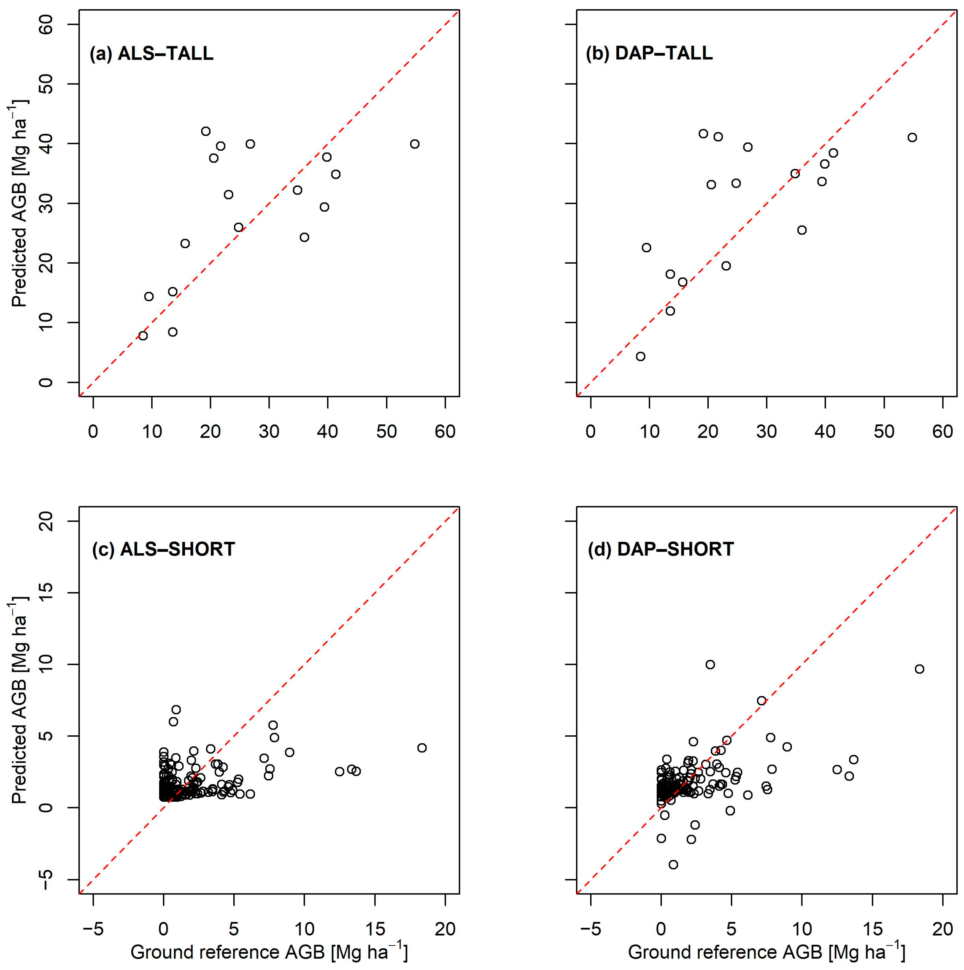
| Stratum | Model | Explanatory Variable | Prediction Model | adj-R2 | RMSE (Mg ha−1) | rel.RMSE (%) |
|---|---|---|---|---|---|---|
| TALL | AGB-ALS | 0.47 | 12.4 | 41.1 | ||
| AGB-DAP | 0.43 | 12.8 | 43.8 | |||
| SHORT | AGB-ALS | 0.15 | 2.47 | 154.2 | ||
| AGB-DAP | 0.27 | 2.28 | 118.1 |
| Stratum * | Model | (Mg ha−1) | (Mg ha−1) | (Mg ha−1) |
|---|---|---|---|---|
| TALL A = 0.97 ha | AGB-ALS | 26.5 | 3.16 | 23.4–29.7 |
| AGB-DAP | 29.2 | 3.13 | 22.9–35.5 | |
| SHORT A = 270.75 ha | AGB-ALS | 2.05 | 0.20 | 1.66–2.45 |
| AGB-DAP | 1.93 | 0.17 | 1.59–2.27 | |
| Total A = 271.72 ha | AGB-ALS | 2.14 | 0.39 | 1.75–2.53 |
| AGB-DAP | 2.03 | 0.34 | 1.68–2.37 |
Disclaimer/Publisher’s Note: The statements, opinions and data contained in all publications are solely those of the individual author(s) and contributor(s) and not of MDPI and/or the editor(s). MDPI and/or the editor(s) disclaim responsibility for any injury to people or property resulting from any ideas, methods, instructions or products referred to in the content. |
© 2023 by the authors. Licensee MDPI, Basel, Switzerland. This article is an open access article distributed under the terms and conditions of the Creative Commons Attribution (CC BY) license (https://creativecommons.org/licenses/by/4.0/).
Share and Cite
Mukhopadhyay, R.; Næsset, E.; Gobakken, T.; Mienna, I.M.; Bielza, J.C.; Austrheim, G.; Persson, H.J.; Ørka, H.O.; Roald, B.-E.; Bollandsås, O.M. Mapping and Estimating Aboveground Biomass in an Alpine Treeline Ecotone under Model-Based Inference. Remote Sens. 2023, 15, 3508. https://doi.org/10.3390/rs15143508
Mukhopadhyay R, Næsset E, Gobakken T, Mienna IM, Bielza JC, Austrheim G, Persson HJ, Ørka HO, Roald B-E, Bollandsås OM. Mapping and Estimating Aboveground Biomass in an Alpine Treeline Ecotone under Model-Based Inference. Remote Sensing. 2023; 15(14):3508. https://doi.org/10.3390/rs15143508
Chicago/Turabian StyleMukhopadhyay, Ritwika, Erik Næsset, Terje Gobakken, Ida Marielle Mienna, Jaime Candelas Bielza, Gunnar Austrheim, Henrik Jan Persson, Hans Ole Ørka, Bjørn-Eirik Roald, and Ole Martin Bollandsås. 2023. "Mapping and Estimating Aboveground Biomass in an Alpine Treeline Ecotone under Model-Based Inference" Remote Sensing 15, no. 14: 3508. https://doi.org/10.3390/rs15143508
APA StyleMukhopadhyay, R., Næsset, E., Gobakken, T., Mienna, I. M., Bielza, J. C., Austrheim, G., Persson, H. J., Ørka, H. O., Roald, B.-E., & Bollandsås, O. M. (2023). Mapping and Estimating Aboveground Biomass in an Alpine Treeline Ecotone under Model-Based Inference. Remote Sensing, 15(14), 3508. https://doi.org/10.3390/rs15143508