Article

A Space-Time Partial Differential Equation Based Physics-Guided Neural Network for Sea Surface Temperature Prediction

1
College of Meteorology and Oceanography, National University of Defense Technology, Changsha 410073, China
2
College of Computer Science and Technology, National University of Defense Technology, Changsha 410073, China
*
Author to whom correspondence should be addressed.
Remote Sens. 2023, 15(14), 3498; https://doi.org/10.3390/rs15143498
Submission received: 30 May 2023 / Revised: 28 June 2023 / Accepted: 3 July 2023 / Published: 12 July 2023
(This article belongs to the Section AI Remote Sensing)

Abstract

:
Sea surface temperature (SST) prediction has attracted increasing attention, due to its crucial role in understanding the Earth’s climate and ocean system. Existing SST prediction methods are typically based on either physics-based numerical methods or data-driven methods. Physics-based numerical methods rely on marine physics equations and have stable and explicable outputs, while data-driven methods are flexible in adapting to data and are capable of detecting unexpected patterns. We believe that these two types of method are complementary to each other, and their combination can potentially achieve better performances. In this paper, a space-time partial differential equation (PDE) is employed to form a novel physics-based deep learning framework, named the space-time PDE-guided neural network (STPDE-Net), to predict daily SST. Comprehensive experiments for SST prediction were conducted, and the results proved that our method could outperform the traditional finite-difference forecast method and several state-of-the-art deep learning and physics-guided deep learning methods.

1. Introduction

Sea surface temperature (SST) plays a fundamental role in understanding global ocean–atmosphere ecosystems and the Earth’s climate system, having significant implications for marine science research [1]. Studying the spatiotemporal distribution and evolution of SST is crucial for fisheries, ocean disaster prevention, and global warming analysis, etc. [2,3]. Moreover, as the lower interface between the ocean and the atmosphere, SST significantly influences atmospheric circulation. For instance, in areas with high SST, low-pressure systems are prone to form, while in regions with low SST, divergent high-pressure systems tend to develop, playing a crucial role in the formation of typhoons (SST exceeding 26 degrees Celsius). However, external factors, such as solar radiation and dynamic elements (momentum fluxes: u-component and v-component), and the insufficiency of data, make SST prediction highly challenging [4]. The existing SST prediction researches are generally divided into physics-based numerical methods and data-based methods [5,6,7].
Physics-based numerical methods are widely applied and typically describe the relationships between oceanic variables using various oceanographic laws and equations. Currently, Hybrid Coordinate Ocean Model (HYCOM) [8], the Regional Ocean Modeling System (ROMS) [9], and Princeton Ocean Model (POM) [10] are commonly used physics-based models in the oceanography field. These numerical methods heavily rely on our understanding of ocean physics and can provide stable and interpretable output results. However, their performance is limited by the incompleteness of our knowledge of ocean physics, such as the initial and boundary conditions of equations, and the complex relationships between many interacting ocean elements.
In contrast to physics-based numerical methods, data-driven methods usually mine important knowledge from historical data, without assuming physical priors [11,12]. Clearly, they can help uncover important patterns in datasets that we still do not fully understand. Among these methods, deep learning has achieved tremendous success in the environmental system modeling domain, maintaining state-of-the-art performance in numerous tasks in recent years [13,14,15,16]. However, it remains unclear how these models produce specific decisions, and physically interpreting these data-driven models is challenging [17,18,19,20,21]. Additionally, in many cases, the available training data for predictive models are insufficient, making it difficult for these models to extract enough useful information from the data to achieve stable outputs and a good performance [20,22,23].
Moreover, most of these deep learning models have inherent flaws, which also constrain their ability to model and predict SST. Traditionally, convolutional neural networks (CNNs), recurrent neural networks (RNNs), and transformer architectures based on self-attention mechanisms have been used as benchmarks for spatiotemporal prediction, since they can reduce temporal and spatial inductive biases [24,25]. However, on the one hand, CNNs are not adept at capturing temporal relationships in data [26]; RNNs struggle with learning long-term sequence dependencies, due to gradient explosion and vanishing problems [27]; and transformer-based models, which calculate self-attention for entire sequences, result in increased computation and are prone to gradient vanishing or explosion [28,29]. Furthermore, the performance of these data-driven methods heavily relies on the availability and quality of labeled data, and they may not fully capture the underlying physical processes governing SST dynamics [30].
Recently, a physics-informed deep learning architecture called PINNs and its variants have played a vital role in addressing the poor interpretability and robustness, and strong data dependency, of traditional deep learning models and have demonstrated certain advantages in materials science, chemistry, astrophysics, hydrology, and fluid mechanics [31,32,33,34]. This architecture incorporates physical laws and boundary conditions into neural networks, making the network outputs conform to the requirements of PDEs [35,36,37]. In addition, compared to the traditional methods, they can handle nonlinearity and high-dimensional problems well [31]. However, although PINN methods have shown enticing potential, PINNs typically rely on the availability of accurate initial conditions and boundary conditions, as well as the completeness and correctness of prior information, which may not always be available in meteorological and oceanographic fields [38,39,40,41,42,43,44,45]. As a result, their applicability in these fields, such as for predicting sea surface temperature, may be limited.
In this study, we propose a variant of the PINN architecture, called STPDE-NET, for spatiotemporal prediction of sea surface temperature (SST). Additionally, we aim to provide an explanation for the prediction mechanism of deep neural networks for SST. To address the issue above, we avoid fixing each term of the partial differential equation (PDE) in the cost function and instead treat them as adjustable parameters. This approach allows us to optimize the entire process by minimizing the distance between the predicted and observed SST values. Through this optimization, we obtain more accurate SST predictions and implicitly accomplish the “parameterization” of the equation. This provides a theoretical explanation for the achievement of model prediction.
The subsequent sections of this paper are organized as follows. Section 2 presents the data used in this study. Section 3 describes the methods applied in this research. Section 4 displays the experimental results. Section 5 provides the discussions and conclusions.

2. Data

The mixed-layer heat budget equation, analyzing heat sources and sinks within the mixed layer, has been widely applied to explore the SST variation process. This equation describes the interactions among oceanic factors affecting the SST variation process. To represent these coupling relationships as best as possible, we need to select sufficiently related variables, to establish a mixed prediction model (physics knowledge combined with deep learning), including solar radiation flux data, sea surface temperature, ocean subsurface temperature, momentum flux-u (or v) component, mixed layer thickness, and longitude and latitude data.
All data need to be preprocessed before being input to the model. Specifically, due to the inconsistent spatiotemporal resolutions of the different data sources, we use one dataset’s resolution as a reference grid and interpolate the remaining data to that grid. Here, we use the spatial resolution of solar radiation data as the spatial reference grid and 12-hours daily average data as the time resolution reference point. Finally, these data are linked along the layer axis, to construct a dataset containing 13 layers to input into our model.
The performance of deep learning models heavily relies on the quantity and quality of the training data. Thus, observation data of real physical processes are the best choice for model training. However, the observation period is usually short, insufficient for adequate sampling, and the phenomenon of missing data affects the model’s capabilities. One possible solution is to use remote sensing data or reanalysis data to increase training quantity and supplement missing data. Therefore, we used the National Centers for Environmental Prediction-Department of Energy Reanalysis 2 (NCEP-DOE R2) (52) and the Copernicus Marine Environment Monitoring Service of the Copernicus Programme of the European Union’s global reanalysis dataset. Additionally, we used NOAA’s OISST as one of our training datasets, to initiate model training. All data cover the period from 2010 to 2019 and were divided into training, validation, and test sets.
All data (raw data or processed data) used in this research have been deposited in a local database and are available if needed. Specific details can be found in Table 1. Moreover, we downloaded the following raw data: the NOAA for providing the OISST-V2 data (https://www.ncei.noaa.gov/products/optimum-interpolation-sst, accessed on 6 December 2021), the National Centers for Environmental Prediction Department of Energy Reanalysis 2 for providing the energy data (https://psl.noaa.gov/data/gridded/data.ncep.reanalysis2.html, accessed on 6 December 2021), and the Copernicus Marine Environment Monitoring Service of the Copernicus Programme of the European Union for providing the reanalysis data (https://marine.copernicus.eu/, accessed on 6 December 2021).

3. Methodology

3.1. Architecture

STPDE-NET: A Mixed Physics and Deep Learning Prediction Model and Its Application in Earth Sciences.
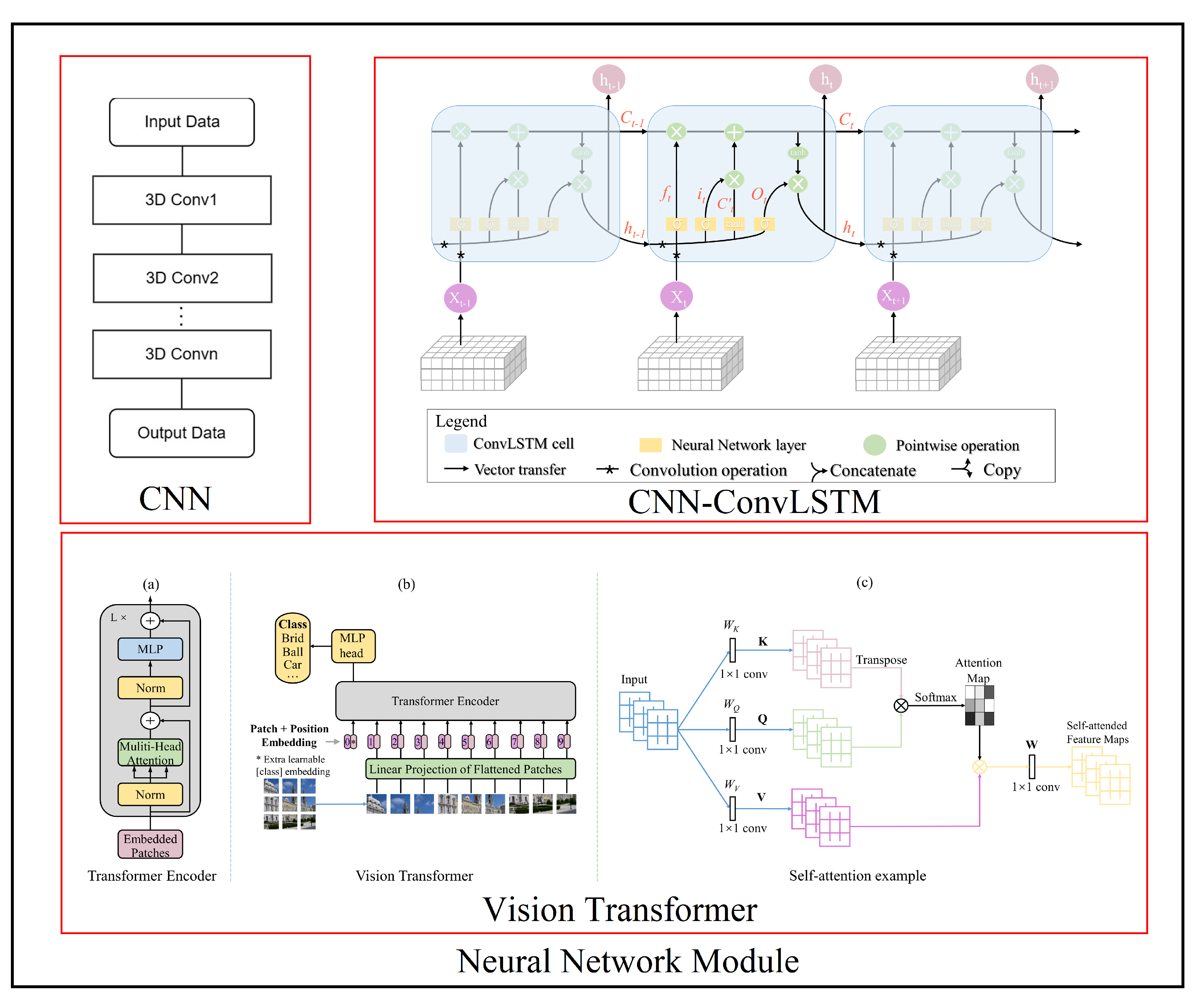
Motivated by the successful application of artificial intelligence (AI) in solving the Birch and Swinnerton-Dyer conjecture, known as the millennium problem in mathematics, and considering the unique characteristics of the widely used mixed-layer heat budget equation, we developed a robust and resilient neural network model called STPDE-NET for sea surface temperature (SST) prediction. Building upon an improved physics-informed neural network (PINN) method, STPDE-NET incorporates a solution process for the equation and consists of several modules: a neural network module, differential solution module, and numerical integration module (refer to Figure 1).
In order to validate the reliability of our method, we applied it to three fundamental deep learning paradigms: convolutional neural network (3D-CNN), recurrent neural network (3D-CNN-ConvLSTM), and vision transformer based on a self-attention mechanism. These models have demonstrated state-of-the-art (SOTA) performance in the field of Earth sciences, particularly in weather forecasting. It is worth noting that the best-performing intelligent weather prediction models in recent years have been based on vision transformer and its variants. The detailed network structures are illustrated in Figure 2.
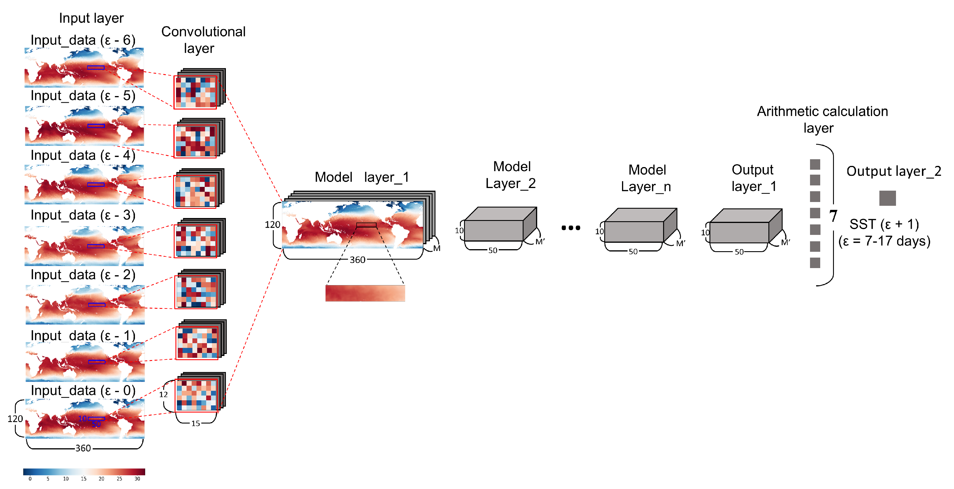
STPDE-NET utilizes seven consecutive days of multi-factor historical information as input predictors (represented as X T i n × C × N l a t × N l o n i n ), where T i n is the time dimension, C represents the number of channels (variables), and N l a t and N l o n correspond to the spatial grid points of the reference field. The input predictors encompass multiple factor variables described by the equation, resulting in 13 channels. Thus, the dimensions of the input data are T i n × C × N l a t × N l o n = 7 × 13 × 6 × 27 . The target predictions consist of the subsequent 10-day scenarios (represented as X i n T o u t × C × N l a t × N l o n ). Following the approach of Ham et al., we train multiple models to output predictions for different future time spans, resulting in dimensions of T o u t × C × N l a t × N l o n = 7 × 10 × 6 × 27 . This process is performed iteratively over ten steps (as depicted in Figure 3).
As illustrated in Figure 3, the input predictors are first transformed using the intrinsic neural network parameters of the model, yielding an intermediate variable for gradient calculation of the input predictors. The intermediate variable is then mapped to the specified expression incorporating equation information on the channel dimension and subsequently integrated forward with respect to the temperature’s time derivative. Finally, the desired prediction field information is obtained. In this process, the selected equation for STPDE-NET (mixed-layer heat budget equation) is not directly solved numerically nor fixed in the cost function, as in the traditional PINN methods. Instead, it is positioned in the intermediate stage between the neural network output and the cost function. This approach harnesses the deep learning capabilities of the neural network to extract valuable information from the data, allowing the model parameters to capture information described by the data but not explicitly present in the equation, thereby enhancing the accuracy of predictions.

3.2. Differential Calculation Module

Similar to methods based on physics-informed neural networks (PINN), the temperature gradient with respect to latitude and longitude can be calculated using the automatic differentiation function of the neural network. In our approach, we utilize the automatic differentiation function to differentiate the model parameters and input coordinates. This process can be summarized as follows:
T t = u T x + v T y = f ( D )
Here, T represents temperature and contains the information of x, y, and t. In this paper, x, y, and t correspond to the longitude, latitude, and time information of T, respectively.
Furthermore, our framework enables the neural network to not only perform traditional difference algorithms (e.g., spectral method, finite element method) but also learn simplified or omitted information from empirical equations through iterative optimization [50,51]. We illustrate the implementation of this process as follows:
u T x + v T y + R α u u x + β v u y + R
In our framework, we optimize the embedded equation and model parameters concurrently. During this process, we obtain an intermediate state quantity named u , which replaces T in the original formula. This step resembles a parametric scheme. In the aforementioned process, we introduce the adaptive parameters α and β for a detailed description. These parameters minimize the discrepancy between prediction values and labels and adaptively adjust the weights. By optimizing the equation itself, they can improve the accuracy of prediction results and compensate for any simplified or missing information in the empirical equation.

3.3. Model Training Strategy

The STPDE-NET prediction model, which combines mixed physics and deep learning approaches, utilizes batch variables as input predictors. Each batch variable represents a span of 7 consecutive days, and the model aims to predict the output fields for the subsequent 1–10 days. The model adopts a state-based prediction strategy, where the current state of all factor information serves as input, and the model simultaneously outputs a single target time step prediction result. This prediction approach implicitly considers the system state’s evolution through the utilization of multi-factor input information.
To comprehensively evaluate the model’s performance in SST prediction, we employ several evaluation criteria: root mean square error (RMSE), Pearson correlation coefficient (PCC), mean absolute error (MAE), mean squared error (MSE), and mean absolute percentage error (MAPE). These measures quantify the deviation between the prediction results and the observed target values, providing a comprehensive assessment of the model’s accuracy.
The RMSE is defined as follows:
R M S E = 1 n i = 1 n ( y i y i ) 2
where y i represents the target SST values, y i means the predicted SST values, y i ¯ denotes the average of the target SST values, and y i ¯ is the mean of the predicted SST values.
An additional set of formulas for calculating the PCC, MAE, MSE, and MAPE of predicted values is provided in the Supplementary materials. The corresponding predicted results for these formulas can be found in Tables S14–S22.
Additionally, to ensure the reproducibility of the experimental results, all experimental results are averaged over five experiments with fixed random seeds of 1–5, to guarantee the stability of the experimental results and enable further comparative analysis.
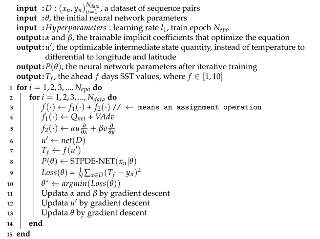
Algorithm 1 implements the training procedure of the STPDE-NET for SST prediction. The trainable implicit coefficients α and β , and the intermediate state quantity u are updated based on the gradient descent function. In our implementation, to make a fair comparison, we selected the model parameters based on traditional data-driven methods. For more detailed parameters, see the Supplementary Material Tables S1–S12.

3.4. Mixed-Layer Heat Budget Equation

The mixed-layer heat budget equation is a valuable tool for understanding the variation of sea surface temperature (SST) through examining heat sources and sinks within the mixed layer. This equation has played a significant role in various oceanic studies, including investigations into the physical mechanisms of SST changes, El Niño-Southern Oscillation (ENSO) mechanisms, and ocean heat wave mechanisms. The equation is mathematically expressed as follows:
T m t T e n d = Q ρ C p h m Q n e t u T m x Z A d v v T m y M A d v w e ( T m T d ) h m V A d v + R
where the terms u, v, and T m indicate the zonal and meridional current velocities and the ocean temperature averaged over the mixed layer depth, respectively. We applied a spatiotemporally varying h m to describe the mixed layer depth, where the marine temperature is 0.5 °C cooler than the surface values. The terms C p = 4000 Jkg 1 K 1 and ρ = 1025 kg m 3 indicate the seawater specific heat and seawater density, respectively. R represents the algebraic expression (without differential calculation) formed by the other variables in the equation; these symbols are used here for convenience only. The terms w e and T d are the vertical ocean current velocity and the seawater temperature below the 10 m bottom of the mixed layer.
Algorithm 1: Training procedure of the STPDE-NET for SST prediction.
Remotesensing 15 03498 i001
The left side of Equation (4) is the mixed-layer ocean temperature tendency (Tend). Q n e t is the net surface heat flux term and indicates the main thermodynamic elements in the process of temperature change. The terms of ZAdv (MAdv and VAdv) are the zonal (meridional and vertical) advection components of the average velocity.

3.5. Extract Knowledge from Data and Optimize Equations

An effective way to learn laws from physical equations (systems) is usually to construct them as a supervised learning task, where the input x i = X u ( i ) (referred to as X ) and the target output y i = Y u ( i ) (referred to as Y ) follow certain mapping laws: X Y . Essentially, this process involves learning a virtual hypothetical equation θ : X Y , with the objective of approximating θ to f. Mathematically, this process can be formulated as an optimization problem, as shown in Equation (5).
u T x + v T y + R α u u x + β v u y + R
However, empirical equations often contain unknown, simplified, omitted, or even inaccurate information. To address this limitation, we propose separating the empirical equation into known and unknown components.
y = f ( x ) = f 1 ( x ) + f 2 ( x )
Here, f 1 ( · ) represents the physical laws that can be accurately understood in the real world, while f 2 ( · ) represents the unknown, simplified, omitted, or inaccurate information in the empirical equations. Consequently, the learning process can be expressed as θ * ( x ) = θ 1 * ( x ) + θ 2 * ( x ) . In this process, we aim to capture the limited physical laws ( θ 2 * ( x ) = θ 2 ( x ) , x X ), while minimizing the loss function, to obtain an equivalent representation θ 1 * ( x ) . We introduce an optimized intermediate state quantity u and calculate its derivative with respect to the original longitude and latitude information. The iterative optimization of the model parameters implicitly optimizes the equation itself. In this way, we completed tasks such as developing the parameterization scheme.

4. Results

4.1. Comprehensive Evaluation of the General Prediction Capabilities of Various Models through Multiple Error Statistical Analyses Based on Spatiotemporal Evolution Characteristics

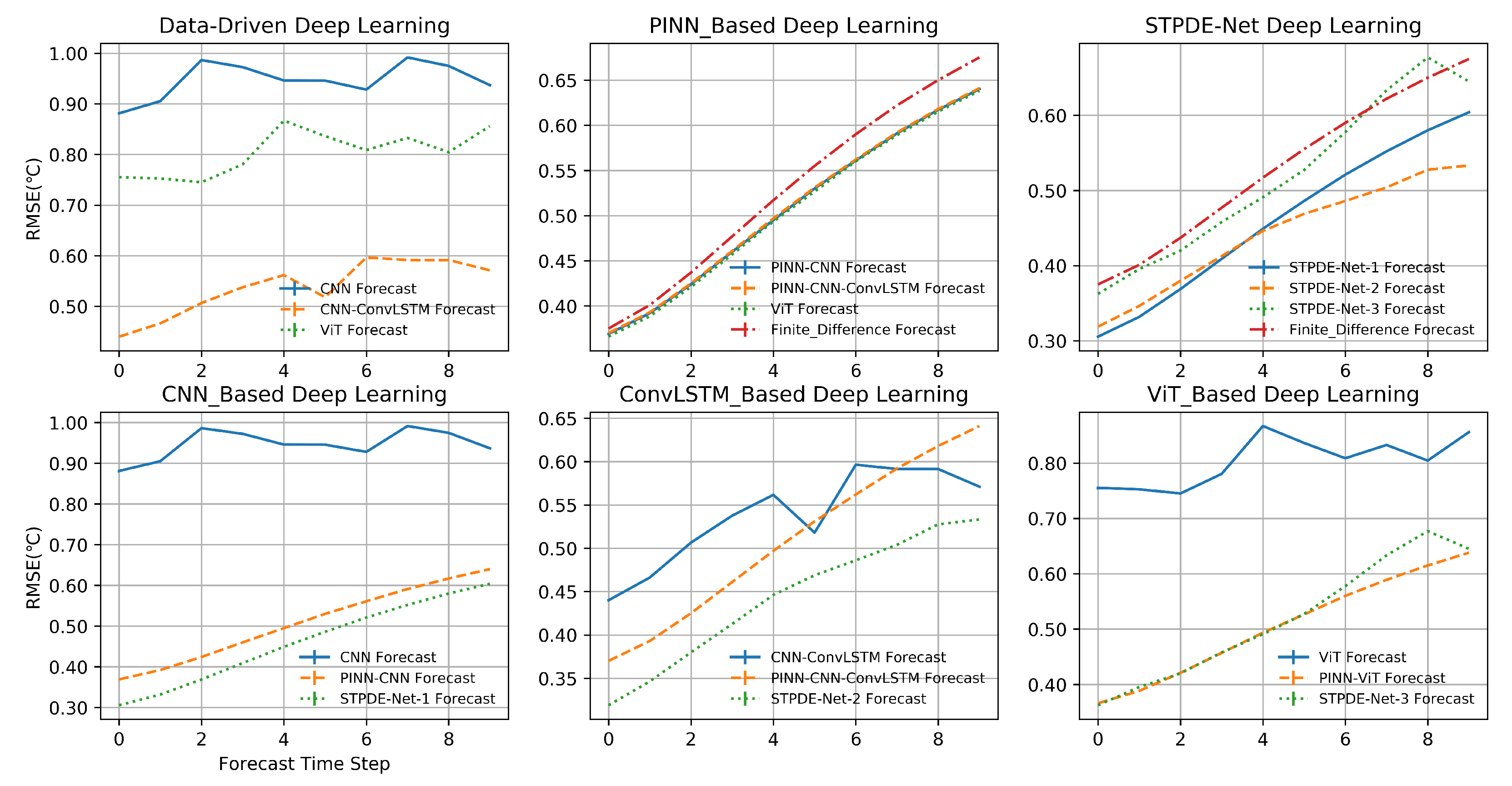
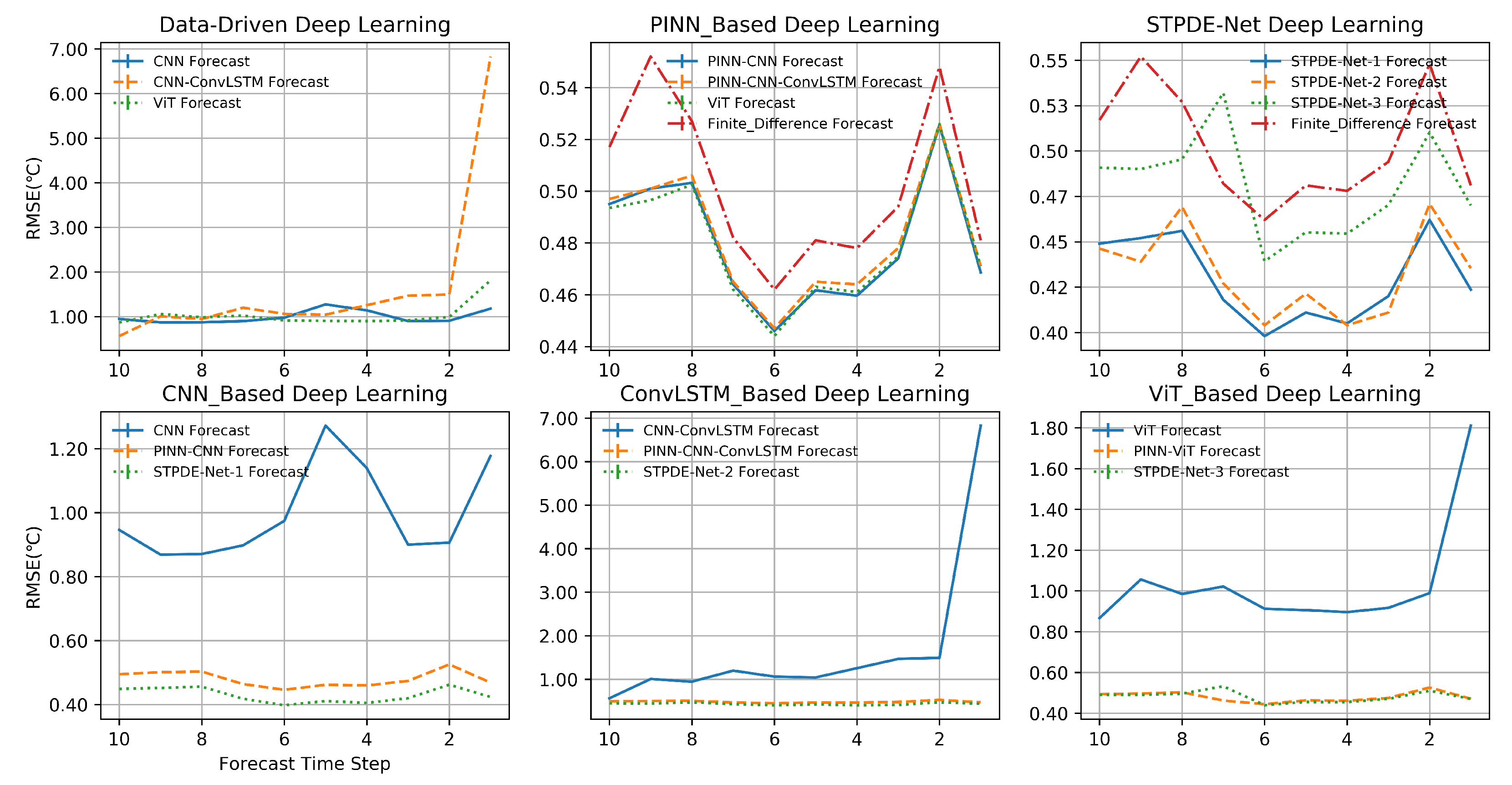
To quantitatively evaluate the prediction capabilities of the various models, we used ERA5 reanalysis data as our label to measure the distance between the predicted target variable (SST) and the label. As shown in Figure 4, we independently conducted 1–10 day forward predictions using multiple models with different time spans. To fully demonstrate the superiority of our proposed method, we compared it to three commonly used data-driven model families, i.e., models based on CNN, RNN, and transformer architectures. For fairness in the comparison, all model parameters were adjusted based on purely data-driven results and retained as hyperparameters for subsequent prediction studies using PINN-based methods and STPDE-NET methods (Tables S2–S13). In addition, we also compared the prediction results of traditional finite difference methods based on numerical differences and global models.
Our study focused on assessing the model’s predictive ability based on the performance in SST prediction and examining how their accumulated prediction error changed over time. For easy reading, we divided the comparison results into six parts based on the different model architectures and implementation methods. We named our methods based on CNN, RNN, and transformer architectures STPDE-NET-1, STPDE-NET-2, and STPDE-NET-3, respectively. Here, we used five metrics to evaluate the SST prediction performance relative to the observed values: root mean square error (RMSE), Pearson’s correlation coefficient (PCC), mean absolute error (MAE), mean squared error (MSE), and mean absolute percentage error (MAPE) (Tables S14–S22).
Figure 4 shows the SST prediction results for different lead times using 10 years of data, demonstrating that STPDE-NET outperformed the traditional data-driven methods, PINN-based methods, and finite difference methods (Figure 1D–F). Specifically, it could create an effective mid-to-long-term SST prediction with a lead time of 10 days, and the prediction error was acceptable. Similarly, these methods all exhibited certain commonalities, such as the accumulation of prediction errors as the forecast time increased. Furthermore, Table 2 shows the improvement of our method compared to the traditional algorithms.

4.2. Sensitivity Experiments Performed for Robustness

In the field of machine learning, the robustness of a model refers to its tolerance for anomalies or errors in the data, which is crucial for determining the model’s reliability and practicality [24,38]. Accordingly, in the field of meteorology and oceanography, the available observational data may be sparse or even unaffordable, severely challenging the application of deep learning models in this field [30]. In this section, we conducted sensitivity experiments, to reveal the representation processes of all methods used.
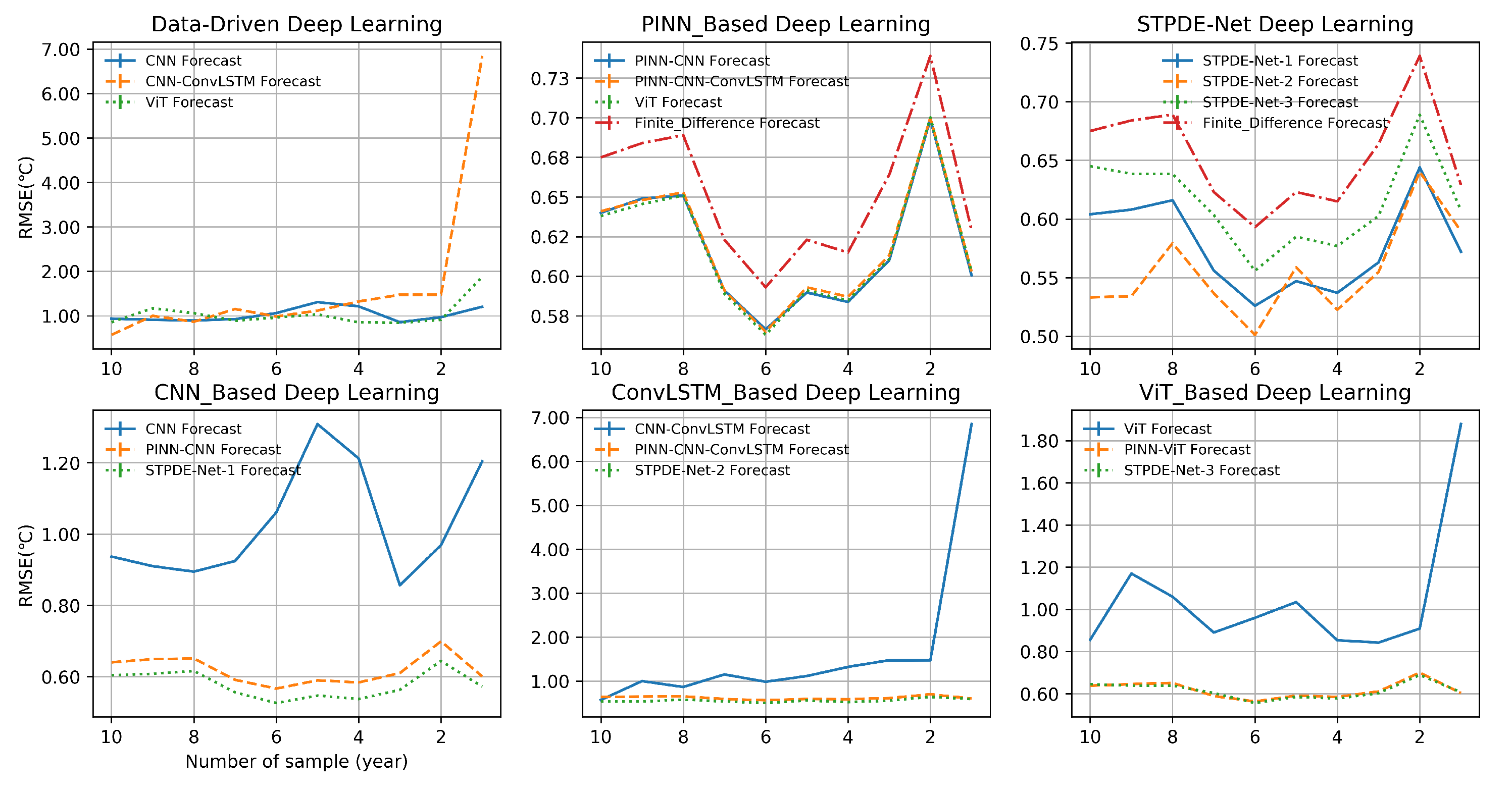
As shown in Figure 5 and Figure 6, we validated the SST forecast effects for 5-day and 10-day leads, respectively, using input data ranging from 10 years to 1 year (for more details, see Figures S1–S9). It was evident that the pure data-driven methods were highly sensitive to input data; in general, as the input data decreases, the error of pure data-driven methods increases and becomes unacceptable. PINN-based methods remain stable, as previously explained, since each term of the PDE in the cost function is always fixed in PINN methods, making it less likely that the prediction performance will change significantly due to data variations. We must note that our method is affected to some extent by data changes, and too little training data may result in a decline in optimization performance. However, it is clear that our method always had a promoting effect on the equation prediction results, and its prediction performance was always superior to that of the traditional PINN-based prediction methods (Table S1).

4.3. Limitation Analysis of Pure Data-Driven Deep Learning Methods

As previously mentioned, deep learning methods driven solely by data demonstrate powerful performance in handling large amounts of structured and unstructured data. However, they still have inherent limitations. The impact of data volume on data-driven models was evident, as shown in Figure 5 and Figure 6. As the input data decreased, the model’s predictive performance decreased. In the field of oceanography, the available observational data are typically sparse and costly. Oceanic observations primarily rely on conventional methods, such as buoys, ship surveys, and fixed platforms, resulting in insufficient observational coverage, particularly in coastal regions of marginal seas and basins. Satellite observations are a good solution. Currently, even high-quality SST observational data, such as those released by NOAA, are only available as daily measurements from September 1981. For instance, phenomena such as ENSO and PDO typically require monthly averaged data as input. However, there are only around 40 years of data (1981–2023), which is approximately equivalent to the volume of daily averaged data for a year and represents a relatively small sample size in our ablation experiments. At this point, the reliability of purely data-driven deep learning methods becomes questionable.
Furthermore, every model has its inherent flaws, and understanding the internal workings of the model also presents challenges. It is difficult to mechanistically explain at which point the reduction of data renders the model unusable, which may be unacceptable for this application scenario [17,18,19,20,21]. For example, when comparing models based on recurrent neural networks (RNNs) and transformers with more parameters (theoretically requiring more input data), it was observed that, due to their gating structure and long-term temporal noise, models based on RNNs experienced a rapid decline in performance, whereas transformer models seemed to be less affected.

4.4. Evaluating the Accuracy of Oceanic Models with Reanalysis SST Data

The question of which type of data is most accurate in the oceanic field remains open-ended. In this study, we used the EC’s reanalysis SST data as a label to evaluate the accuracy of the numerical models and various deep learning methods. Figure 7 formalizes the error between the HYCOM output model data and the EC’s reanalysis data from 2010 to 2017. The left panel shows the difference between all SSTs and the label in the study area during this time period, while the right panel averages the spatial data, while retaining the time series information. It is evident that even the currently recognized accurate numerical models still exhibited numerical drift (the error bars in the left panel are around 6), and it is not difficult to see that the absolute values of most errors exceeded 1 °C, indicating that there is still room for improvement in the model. Nevertheless, it is worth noting that HYCOM can still accurately depict a system’s evolution process after averaging the data over the domain. It should be mentioned that we chose the years 2010 to 2017 because HYCOM only provides data for 2009 to 2017 in this channel.

4.5. Empirical Analyses Showing PINN Failure Modes

Compared to our proposed method, PINN-based models seemed to “fail”. Here, we provide some possible reasons for this observation. First, it should be clear that for this experiment, the PINN-based methods were superior to the traditional equation-solving methods using finite differences (Figure 4, Figure 5 and Figure 6). This may have been because the automatic differentiation feature of neural networks can avoid the accuracy issues and discretization errors that may occur during the numerical differentiation process. However, in general, PINN methods usually embed physical prior information (usually PDEs) into the cost function of deep learning, where the loss function consists of two parts: a data fitting term and physical equation term. The physical equation term is obtained by incorporating the physical equation into the neural network model, forcing it to satisfy physical laws. As a result, this method generally has stronger generalization and some interpretability compared to traditional purely data-driven deep learning methods. However, it also has certain drawbacks, such as being constrained by initial conditions. For problems in the natural world that conform to fluid mechanics (large-scale fluids generally involve turbulent processes), the initial and boundary conditions may be unknown, necessitating the use of sampling or other methods to estimate these conditions, which may introduce sampling errors [39].
In this study, the mixed-layer heat budget equation was used to explore the SST variation process through analyzing heat sources and sinks in the mixed layer and has played an essential role in various oceanic fields, such as the study of SST change mechanisms, ENSO mechanism research, and marine heatwave mechanism research [40]. However, the equation itself has an elusive residual term R (possibly due to the uncertainty caused by large-scale mixing (a turbulent process) and cumulative errors brought about by empirical parameter selection during equation modeling), indicating that there is room for further optimization of the equation [39]. Moreover, the equation does not have initial or boundary conditions. Therefore, when using PINN-based methods for prediction, the equation’s flaws are also incorporated into the PINN method. Since the PINN method keeps each term of the PDE fixed in the cost function, data learning cannot optimize the equation itself and only strives to satisfy the solution described by the equation.
The STPDE-NET method incorporates PDEs with adjustable parameters into the cost function. By minimizing the distance between the predicted target variable and the observations, it optimizes the entire process and corrects some uncertain terms in the physical equation through data. On the one hand, this leverages the neural network’s ability to deeply mine valuable information from data; on the other hand, it avoids the impact of uncertain terms in PINN on the results.

4.6. Possible Mechanism Analysis for Interpretability

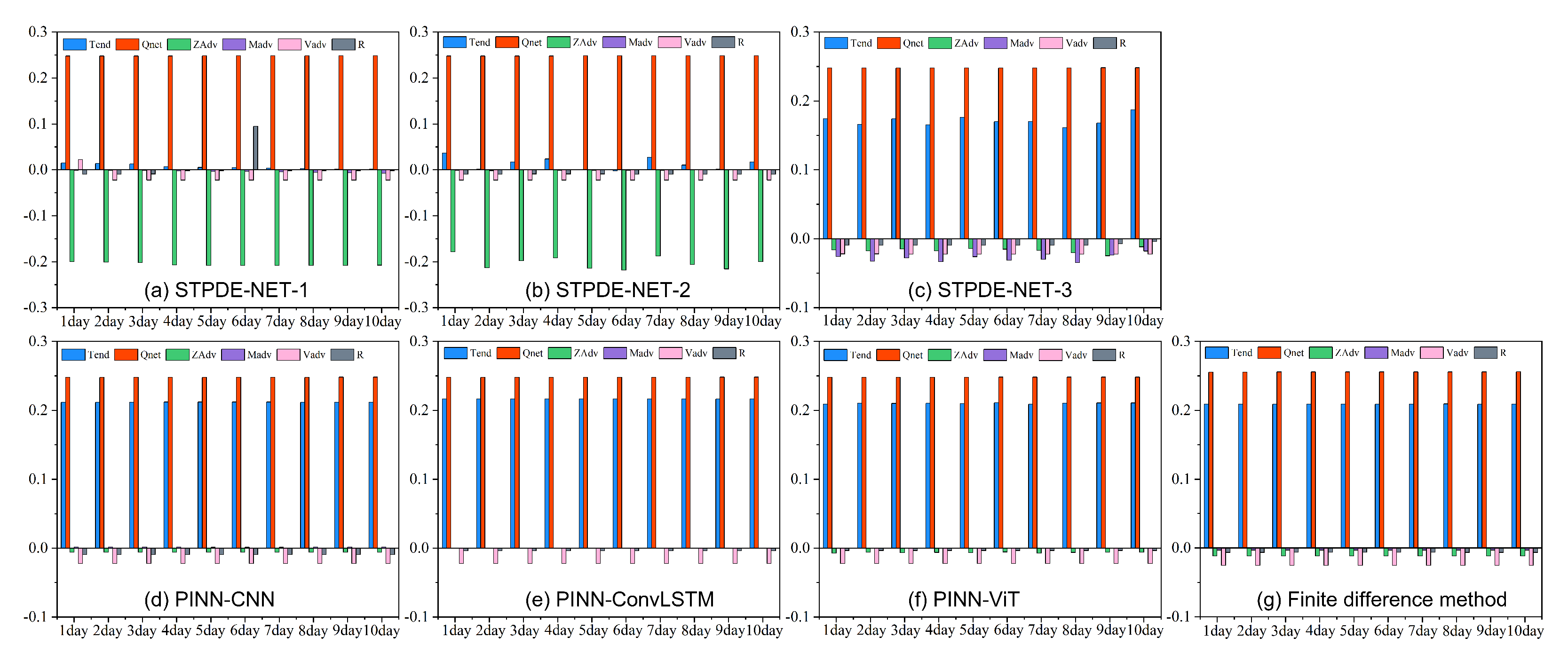
To better understand our proposed method, we divide the equation guiding our experiment (Equation (3)) into six parts: a tendency term (Tend); net surface heat flux term ( Q n e t ); and the zonal, meridional, and vertical advection terms (ZAdv, MAdv, and VAdv). R represents the error residual, originating from cumulative errors caused by the selection of numerous empirical parameters during equation modeling and the uncertainty of oceanic turbulence processes [39]. For the various data samples and different prediction times, STPDE-NET-1 and STPDE-NET-2 achieved the best RMSE results. As shown in Figure 8a,b, the ZAdv term had a significant increase and balanced the Q n e t term, resulting in a smaller Tend. In other experiments, the ZAdv term was relatively small, and the trend term was only dominated by Q n e t . In terms of the prediction results, it seemed that the increase of the ZAdv term helped to more accurately characterize the equation and obtain more precise prediction results. This is because the mixed-layer heat budget equation cannot capture the deepening and cooling phenomena of the mixed layer caused by large-scale mixing (a turbulent process that has an impact on ocean dynamics). Only when the mixed layer is entirely isothermal, does this cooling and dilution warming effect not exist, which is evidently unrealistic for the actual ocean [39]. For small regional scales, the temperature varies with latitude due to geographical regulation. In this study, our method demonstrated a relatively small but noticeable improvement on the MAdv term, which is consistent with common sense. In addition, in small-scale and short-term events, and some crucial dynamic processes, such as wind- and tide-induced vertical mixing or entrainment, the vertical advection term VAdv may play a key role in changing the sea surface temperature. However, in our study, it seemed that VAdv produced a smaller improvement on the equation, as our research focused on the average state of sea surface temperature over a ten-year range.
Furthermore, we found that in PINN-based deep learning methods, each term of the PDE was always fixed in the cost function. This indicates some limitations of the PINN method. As can be seen from the figure, the PINN-based method, compared to finite differences, minimized the role of the ZAdv term. This could have been a major factor leading to the instability of PINN predictions in our experiment, as it considers less turbulence-induced uncertainty learned from the data.

5. Discussion and Conclusions

At present, real-time SST predictions mainly rely on physics-based dynamical models and data-driven methods, but there are still significant biases and uncertainties that greatly hinder medium-to-long-term SST forecasting [34]. Recent advancements in DL models based on physics-informed neural networks (PINNs) provide a promising approach for nonlinear system modeling, with potential applications in SST prediction. However, due to the inherent limitations of PINNs and challenges in prior knowledge completeness in the atmospheric and oceanographic fields, accurate SST evolution prediction using PINN models still requires substantial improvements.
Inspired by the successful application of AI in helping mathematicians solve the millennium problem of the Birch and Swinnerton-Dyer conjecture, we developed a neural network combining physical priors with data-driven methods, called STPDE-NET. By dynamically inserting the mixed-layer heat budget equation (widely used to analyze heat sources and sinks within the mixed layer to study SST changes) into the network structure, it could be used for SST modeling. Our model’s unique ability to optimize the equation’s attributes from data, by adjusting the minimization of the distance between the predicted target variable and the observations, establishes multivariate interconnections. The effectiveness and superiority of STPDE-NET for SST mid-term prediction were demonstrated, and it could counteract the adverse effects of having limited input data.
Specifically, the STPDE-NET model cold correct some unclear terms in the physical equations through data. It was compared to the traditional finite difference method as a benchmark, and the correction effect is summarized in Table 2. This represents an advancement, as completely accurate equations describing elemental dynamic or thermodynamic processes may not always be available in the atmospheric and oceanographic fields. Our method not only improved the SST prediction performance but also mechanistically analyzed the increased ZAdv term learned by STPDE-NET from data, with a larger ZAdv corresponding to smaller prediction errors. Moreover, sensitivity experiments were conducted to demonstrate the robustness of our model and highlight the effectiveness of STPDE-NET in alleviating DL’s high data dependence.
The black-box nature of DL models is the primary obstacle to their interpretability in SST-related prediction. Here, we developed a physics-inclusive DL model (i.e., STPDE-NET) that captures the “optimized” state of the equation using data, including descriptive information corresponding to each part of the equation. In terms of interpretability, there have been no previous reports on using PINN methods for SST prediction, let alone taking a step further by combining the advantages of PINNs and DL, “optimizing” the mixed-layer heat budget equation, and achieving more accurate SST predictions. We also provided explanations for some of the “optimized” mechanisms; for example, in small-scale short-time-span events, due to some crucial dynamic processes, such as wind- and tide-induced vertical mixing or entrainment, the vertical advection term (VAdv) may play a key role in changing sea surface temperature. However, in our research, we found that VAdv’s improvement of the equation was relatively small, as our study covered the average state of sea surface temperature over a decade. Additionally, we conducted sensitivity experiments, to explore the description of common meteorological factors for temperature, and which are not included in any term of the equation, allowing us to capture potentially useful precursors of SST evolution. Therefore, our model can, not only provide methods to explore SST coupled dynamics, but also offer insights into the fundamental factors affecting SST prediction.
There are still aspects of the proposed STPDE-NET model that require further improvement. On the one hand, to enhance the method’s overall performance, an additional neural network could be trained to learn and transfer parameters across different time steps, thereby improving the accuracy and efficiency of the solutions. On the other hand, continuous-form data models could be designed to describe the spatiotemporal data variation information within oceanic datasets, potentially addressing the “spatiotemporal” PDE problem more effectively, which is worth further investigation based on our STPDE-NET modeling. Currently, continuous-form data models typically require numerical methods to solve PDEs, which is a complex issue that demands a balance between solution accuracy and computational efficiency. Determining how to strike this balance will one of the directions of our future efforts.
Additionally, we aim to explore the significance of our research in the context of climate change. It is widely known that accurate prediction of sea surface temperature (SST) is crucial, as many extreme events such as typhoons, El Niño, and marine heatwaves are closely related to SST. Our study focused on improving the accuracy of local (medium- to long-term) SST predictions. We believe that this could be beneficial for decadal SST predictions, as large-scale predictions are inevitably accompanied by the accumulation of small-scale errors. Furthermore, investigating extreme events such as El Niño and marine heatwaves is inevitably associated with large-scale SST predictions, which may have implications for environmental changes.
In summary, our deep learning model, which combines the strengths of physical priors and deep learning, successfully achieved medium- to long-term SST-related predictions and demonstrated a robust performance. This indicates that the model has significant potential for climate modeling. Relevant variants could be connected to different equations in the atmospheric and oceanographic fields and applied to other variables or climate prediction tasks. They are expected to become widely accepted DL models in the Earth sciences domain.

Supplementary Materials

The following supporting information can be downloaded at: https://www.mdpi.com/article/10.3390/rs15143498/s1, Table S1: Design of the architecture of the deep CNN neural network model, Table S2: Prediction results (mean ± std) for 1-day ahead with different l_cnn settings, Table S3: Prediction results (mean ± std) for 1-day ahead with different hidden_cnn settings, Table S4: Prediction results (mean ± std) for 1-day ahead with different lr_cnn settings, Table S5: Prediction results (mean ± standard) for 1-day ahead with different e l s t m settings, Table S6: Prediction results (mean ± standard) for 1-day ahead with different l l s t m settings, Table S7: Prediction results (mean ± standard) for 1-day ahead with different hidden_lstm settings, Table S8: Prediction results (mean ± standard) for 1-day ahead with different lr_lstm settings, Table S9: Prediction results (mean ± standard) for 1-day ahead with different e V i T settings, Table S10: Prediction results (mean ± standard) for 1-day ahead with different h V i T settings, Table S11: Prediction results (mean ± standard) for 1-day ahead with different d V i T settings, Table S12: Prediction results (mean ± standard) for 1-day ahead with different lr_ViT settings, Table S13: MAE, MSE, MAPE, and r (mean ± std) of the SST prediction using 10 years data and various methods for different prediction horizons (1–10 days), Table S14: MAE, MSE, MAPE, and r (mean ± std) of the SST prediction using 9 years data and various methods for different prediction horizons (1–10 days), Table S15: MAE, MSE, MAPE, and r (mean ± std) of the SST prediction using 8 years data and various methods for different prediction horizons (1–10 days), Table S16: MAE, MSE, MAPE, and r (mean ± std) of the SST prediction using 7 years data and various methods for different prediction horizons (1–10 days), Table S17: MAE, MSE, MAPE, and r (mean ± std) of the SST prediction using 6 years data and various methods for different prediction horizons (1–10 days), Table S18: MAE, MSE, MAPE, and r (mean ± std) of the SST prediction using 5 years data and various methods for different prediction horizons (1–10 days), Table S19: MAE, MSE, MAPE, and r (mean ± std) of the SST prediction using 4 years data and various methods for different prediction horizons (1–10 days), Table S20: MAE, MSE, MAPE, and r (mean ± std) of the SST prediction using 3 years data and various methods for different prediction horizons (1–10 days), Table S21: MAE, MSE, MAPE, and r (mean ± std) of the SST prediction using 2 years data and various methods for different prediction horizons (1–10 days), Table S22: MAE, MSE, MAPE, and r (mean ± std) of the SST prediction using 1 years’s data and various methods for different prediction horizons (1–10 days), Figure S1: RMSE of the SST prediction using 9 years data and various methods for different prediction horizons (1–10 days), Figure S2: RMSE of the SST prediction using 8 years data and various methods for different prediction horizons (1–10 days), Figure S3: RMSE of the SST prediction using 7 years data and various methods for different prediction horizons (1–10 days), Figure S4: RMSE of the SST prediction using 6 years data and various methods for different prediction horizons (1–10 days), Figure S5: RMSE of the SST prediction using 5 years data and various methods for different prediction horizons (1–10 days), Figure S6: RMSE of the SST prediction using 4 years data and various methods for different prediction horizons (1–10 days), Figure S7: RMSE of the SST prediction using 3 years data and various methods for different prediction horizons (1–10 days), Figure S8: RMSE of the SST prediction using 2 years data and various methods for different prediction horizons (1–10 days), Figure S9: RMSE of the SST prediction using 1 year’s data and various methods for different prediction horizons (1–10 days), Figure S10: MSE of the SST prediction using 10 year’s data and various methods for different prection horizons (1–10 days), Figure S11: MSE of the SST prediction using 9 year’s data and various methods for different prection horizons (1–10 days), Figure S12: MSE of the SST prediction using 8 year’s data and various methods for different prection horizons (1–10 days), Figure S13: MSE of the SST prediction using 7 year’s data and various methods for different prection horizons (1–10 days), Figure S14: MSE of the SST prediction using 6 year’s data and various methods for different prection horizons (1–10 days), Figure S15: MSE of the SST prediction using 5 year’s data and various methods for different prection horizons (1–10 days), Figure S16: MSE of the SST prediction using 4 year’s data and various methods for different prection horizons (1–10 days), Figure S17: MSE of the SST prediction using 3 year’s data and various methods for different prection horizons (1–10 days), Figure S18: MSE of the SST prediction using 2 year’s data and various methods for different prection horizons (1–10 days), Figure S19: MSE of the SST prediction using 1 year’s data and various methods for different prection horizons (1–10 days), Figure S20: 5-day lead MSE for SST prediction (2010–2019), Figure S21: 10-day lead MSE for SST prediction (2010–2019), Figure S22: MAE of the SST prediction using 10 year’s data and various methods for different prediction horizons (1–10 days), Figure S23: MAE of the SST prediction using 9 year’s data and various methods for different prediction horizons (1–10 days), Figure S24: MAE of the SST prediction using 8 year’s data and various methods for different prediction horizons (1–10 days), Figure S25: MAE of the SST prediction using 7 year’s data and various methods for different prediction horizons (1–10 days), Figure S26: MAE of the SST prediction using 6 year’s data and various methods for different prediction horizons (1–10 days), Figure S27: MAE of the SST prediction using 5 year’s data and various methods for different prediction horizons (1–10 days), Figure S28: MAE of the SST prediction using 4 year’s data and various methods for different prediction horizons (1–10 days), Figure S29: MAE of the SST prediction using 3 year’s data and various methods for different prediction horizons (1–10 days), Figure S30: MAE of the SST prediction using 2 year’s data and various methods for different prediction horizons (1–10 days), Figure S31: MAE of the SST prediction using 1 year’s data and various methods for different prediction horizons (1–10 days), Figure S32: 5-day lead MAE for SST prediction (2010–2019), Figure S33: 10-day lead MAE for SST prediction (2010–2019), Figure S34: MAPE of the SST prediction using 10 year’s data and various methods for different prediction horizons (1–10 days), Figure S35: MAPE of the SST prediction using 9 year’s data and various methods for different prediction horizons (1–10 days), Figure S36: MAPE of the SST prediction using 8 year’s data and various methods for different prediction horizons (1–10 days), FIgure S37: MAPE of the SST prediction using 7 year’s data and various methods for different prediction horizons (1–10 days), Figure S38: MAPE of the SST prediction using 6 year’s data and various methods for different prediction horizons (1–10 days), FIgure S39: MAPE of the SST prediction using 5 year’s data and various methods for different prediction horizons (1–10 days), Figure S40: MAPE of the SST prediction using 4 year’s data and various methods for different prediction horizons (1–10 days), FIgure S41: MAPE of the SST prediction using 3 year’s data and various methods for different prediction horizons (1–10 days), Figure S42: MAPE of the SST prediction using 2 year’s data and various methods for different prediction horizons (1–10 days), Figure S43: MAPE of the SST prediction using 1 year’s data and various methods for different prediction horizons (1–10 days), Figure S44: 5-day lead MAPE for SST prediction (2010–2019), Figure S45: 10-day lead MAPE for SST prediction (2010–2019), Figure S46: Correlation coefficient of the SST prediction using 10 year’s data and various methods for different prediction horizons (1–10 days), Figure S47: Correlation coefficient of the SST prediction using 9 year’s data and various methods for different prediction horizons (1–10 days), Figure S48: Correlation coefficient of the SST prediction using 8 year’s data and various methods for different prediction horizons (1–10 days), Figure S49: Correlation coefficient of the SST prediction using 7 year’s data and various methods for different prediction horizons (1–10 days), Figure S50: Correlation coefficient of the SST prediction using 6 year’s data and various methods for different prediction horizons (1–10 days), Figure S51: Correlation coefficient of the SST prediction using 5 year’s data and various methods for different prediction horizons (1–10 days), Figure S52: Correlation coefficient of the SST prediction using 4 year’s data and various methods for different prediction horizons (1–10 days), Figure S53: Correlation coefficient of the SST prediction using 3 year’s data and various methods for different prediction horizons (1–10 days), Figure S54: Correlation coefficient of the SST prediction using 2 year’s data and various methods for different prediction horizons (1–10 days), FIgure S55: Correlation coefficient of the SST prediction using 1 year’s data and various methods for different prediction horizons (1–10 days), Figure S56: 5-day lead Correlation coefficient for SST prediction (2010–2019), Figure S57: 10-day lead Correlation coefficient for SST prediction (2010–2019).

Author Contributions

T.Y. performed the conceptualization, conducted the research, and wrote the original draft; J.Z. performed the writing, review, and editing; K.R. performed the supervision, review, and funding acquisition; W.W. performed the validation; J.L. performed the review; X.W. performed the data curation, and X.L. performed the review and editing. All authors have read and agreed to the published version of the manuscript.

Funding

This work was supported in part by the science and technology innovation Program of Hunan Province (2022RC3070), the Scientific Research Program of the National University of Defense Technology (No. ZK22-13), and the Hunan Provincial Science and Technology Innovation Leading Talent Fund. We also thank OpenI Community (https://open.pcl.ac.cn, accessed on 6 December 2021) for providing GPUs to conduct experiments.

Data Availability Statement

The source code generated and used for this study is publicly available for download at (https://github.com/ytkmy5555/STPDE_NET.git, accessed on 6 December 2021).

Conflicts of Interest

The authors declare no conflict of interest.

Abbreviations

The following abbreviations are used in this manuscript:
SSTSea Surface Temperature
HYCOMHybrid Coordinate Ocean Mode
ROMsRegional Ocean Modeling System
POMPrinceton Ocean Model
CNNConvolutional Neural Network
RNNRecurrent Neural Network
VITVision Transformer
PINNPhysics-informed deep learning
STPDE-NETSpace-Time Partial Differential Equation-Neural Network
PDEPartial Differential Equation

References

  1. Sun, C.; Kucharski, F.; Kang, I.S.; Wang, C.; Ding, R.; Xie, F. Recent Acceleration of Arabian Sea Warming Induced by the Atlantic-Western Pacific Trans-basin Multidecadal Variability. Geophys. Res. Lett. 2019, 46, 123–456. [Google Scholar] [CrossRef]
  2. Ren, H.H.; Dudhia, J.; Li, H. Large-Eddy Simulation of Idealized Hurricanes at Different Sea Surface Temperatures. J. Adv. Model. Earth Syst. 2020, 12, 1–9. [Google Scholar] [CrossRef]
  3. Stuart-Menteth, A.C.; Robinson, I.S.; Challenor, P.G. A global study of diurnal warming using satellite-derived sea surface temperature. J. Geophys. Res. Part C Oceans 2003, 108, 3155. [Google Scholar] [CrossRef]
  4. L’Heureux, M.L.; Tippett, M.K.; Wang, W.Q. Prediction Challenges From Errors in Tropical Pacific Sea Surface Temperature Trends. Front. Clim. 2022, 4, 837483. [Google Scholar] [CrossRef]
  5. Borgne, P.L.; Roquet, H.; Merchant, C.J. Estimation of Sea Surface Temperature from the Spinning Enhanced Visible and Infrared Imager, improved using numerical weather prediction. Remote Sens. Environ. 2011, 4, 55–65. [Google Scholar] [CrossRef]
  6. Minnett, P.J.; Azcárate, A.A.; Corlett, T.M.; Cuervo, J.V. Half a century of satellite remote sensing of sea-surface temperature. Remote Sens. Environ. 2019, 233, 111366. [Google Scholar] [CrossRef]
  7. Zhang, X.; Li, Y.; Frery, A.C.; Ren, P. Sea Surface Temperature Prediction with Memory Graph Convolutional Networks. IEEE Geosci. Remote Sens. Lett. 2022, 19, 8017105. [Google Scholar] [CrossRef]
  8. Chassignet, E.P.; Hurlburt, H.E.; Smedstad, O.M.; Halliwell, G.R.; Hogan, P.J.; Wallcraft, A.J.; Baraille, R.; Bleck, R. The HYCOM (HYbrid Coordinate Ocean Model) data assimilative system. J. Mar. Syst. 2007, 65, 60–83. [Google Scholar] [CrossRef]
  9. Shchepetkin, A.F.; Mcwilliams, J.C. The regional oceanic modeling system (ROMS): A split-explicit, free-surface, topography-following-coordinate oceanic model. Ocean. Model. 2005, 9, 347–404. [Google Scholar] [CrossRef]
  10. Mellor, G.L.; Blumberg, A.F. Modeling Vertical and Horizontal Diffusivities with the Sigma Coordinate System. Mon. Weather Rev. 2003, 113, 1379–1383. [Google Scholar] [CrossRef]
  11. Chen, X.W.; Lin, X.T. Big Data Deep Learning: Challenges and Perspectives. IEEE Access 2014, 2, 514–525. [Google Scholar] [CrossRef]
  12. Ogut, M.; Bpsch-Liuis, X.; Reising, S.C. A Deep Learning Approach for Microwave and Millimeter-Wave Radiometer Calibration. IEEE Trans. Geosci. Remote Sens. 2019, 57, 5344–5355. [Google Scholar] [CrossRef]
  13. He, K.M.; Zhang, X.Y.; Ren, S.Q.; Sun, J. Deep Residual Learning for Image Recognition. In Proceedings of the 2016 IEEE Conference on Computer Vision and Pattern Recognition (CVPR), Las Vegas, NV, USA, 26 June–1 July 2016; pp. 770–778. [Google Scholar]
  14. Daniel, W.O.; Julian, R.M.; Jugal, K.K. A Survey of the Usages of Deep Learning for Natural Language Processing. IEEE Trans. Neural Netw. Learn. Syst. 2021, 32, 604–624. [Google Scholar]
  15. Wang, X.; Iwabuchi, H.; Yamashita, T. Cloud identification and property retrieval from Himawari-8 infrared measurements via a deep neural network. Remote Sens. Environ. 2022, 275, 113026. [Google Scholar] [CrossRef]
  16. Liu, J.; Tang, Y.M.; Wu, Y.L.; Li, T.; Wang, Q.; Chen, D.K. Forecasting the Indian Ocean Dipole With Deep Learning Techniques. Geophys. Res. Lett. 2021, 48, e2021GL094407. [Google Scholar] [CrossRef]
  17. Ghorbani, A.; Ouyang, D.; Abid, A.; He, B.; Chen, J.H.; Harrington, R.A.; Liang, D.H.; Ashley, E.A.; Zou, J.Y. Deep learning interpretation of echocardiograms. NPJ Digit. Med. 2020, 3, 10. [Google Scholar] [CrossRef] [Green Version]
  18. Iravani, S.; Conrad, T.O.F. An Interpretable Deep Learning Approach for Biomarker Detection in LC-MS Proteomics Data. IEEE/ACM Trans. Comput. Biol. Bioinform. 2022, 20, 151–161. [Google Scholar] [CrossRef]
  19. Kong, X.; Ge, Z. Deep PLS: A Lightweight Deep Learning Model for Interpretable and Efficient Data Analytics. IEEE Trans. Geosci. Remote Sens. 2022, 3154090. [Google Scholar] [CrossRef]
  20. Meng, Y.X.; Rigall, E.; Chen, X.E.; Gao, F.; Dong, J.Y.; Chen, S. Physics-Guided Generative Adversarial Networks for Sea Subsurface Temperature Prediction. IEEE Trans. Neural Netw. Learn. Syst. 2022, 1–14. [Google Scholar] [CrossRef]
  21. Daw, A.; Karpatne, A.; Watkins, W.; Read, J.; Kumar, V. Physics-guided Neural Networks (PGNN): An Application in Lake Temperature Modeling. arXiv 2017, arXiv:1710.11431. [Google Scholar]
  22. Yadav, A.; Vishwakarma, D.K. Sentiment analysis using deep learning architectures: A review. Artif. Intell. Rev. 2020, 53, 4335–4385. [Google Scholar] [CrossRef]
  23. Chattopadhyay, A.; Mustafa, M.; Hassanzadeh, P.; Bach, E.; Kashinath, K. Towards physics-inspired data-driven weather forecasting: Integrating data assimilation with a deep spatial-transformer-based U-NET in a case study with ERA5. Geosci. Model Dev. 2022, 15, 2221–2237. [Google Scholar] [CrossRef]
  24. Yann, L.C.; Bengio, Y.S.; Hinton, G. Deep learning. Nature 2015, 521, 436–444. [Google Scholar]
  25. Raghu, M.; Schmidt, E. A Survey of Deep Learning for Scientific Discovery. arXiv 2020, arXiv:2003.11755. [Google Scholar]
  26. Ham, Y.G.; Kim, J.H.; Luo, J.J. Deep learning for multi-year ENSO forecasts. Nature 2020, 573, 568–572. [Google Scholar] [CrossRef]
  27. Xiao, C.J.; Chen, N.C.; Hu, C.L.; Wang, K.; Gong, J.Y.; Chen, Z.Q. Short and mid-term sea surface temperature prediction using time-series satellite data and LSTM-AdaBoost combination approach. Remote Sens. Environ. 2019, 233, 111358. [Google Scholar] [CrossRef]
  28. Vaswani, A.; Shazeer, N.; Paramar, N.; Uszkoreit, J.; Jones, L.; Gomez, A.N.; Kaiser, L.; Polosukhin, I. Attention Is All You Need. In Proceedings of the 31st Conference on Neural Information Processing Systems, Long Beach, CA, USA, 4–9 December 2017; pp. 6000–6010. [Google Scholar]
  29. Alexey, D.; Lucas, B.; Alexander, K.; Dirk, W.; Zhai, X.H.; Thom, U.; Mostafa, D.; Matthias, M.; Georg, H.; Sylvain, G.; et al. An Image Is Worth 16 × 16 Words: Transformers for Image Recognition at Scale. In Proceedings of the 2021 IEEE International Conference on Learning Representations (ICLR), Vitural, 3–7 May 2021; pp. 1–22. [Google Scholar]
  30. Zhou, L.; Zhang, R.H. A self-attention–based neural network for three-dimensional multivariate modeling and its skillful ENSO predictions. Sci. Adv. 2023, 9, eadf2827. [Google Scholar] [CrossRef]
  31. Raissi, M.; Perdikaris, P.; Karniadakis, G.E. Physics-informed neural networks: A deep learning framework for solving forward and inverse problems involving nonlinear partial differential equations. J. Comput. Phys. 2019, 378, 686–707. [Google Scholar] [CrossRef]
  32. Nguyen, T.N.K.; Dairay, T.; Meunier, R.; Mougeot, M. Physics-informed neural networks for non-Newtonian fluid thermo-mechanical problems: An application to rubber calendering process. Eng. Appl. Artif. Intell. 2022, 114, 105176. [Google Scholar] [CrossRef]
  33. Bihlo, A.; Popovych, R.O. Physics-informed neural networks for the shallow-water equations on the sphere. J. Comput. Phys. 2022, 456, 111024. [Google Scholar] [CrossRef]
  34. Yuan, T.K.; Zhu, J.X.; Ren, K.J.; Wang, W.X.; Wang, X.; Li, X.Y. Neural Network Driven by Space-time Partial Differential Equation for Predicting Sea Surface Temperature. In Proceedings of the 2022 IEEE International Conference on Data Mining, Orlando, FL, USA, 28 November–1 December 2022; pp. 656–665. [Google Scholar]
  35. Zhang, X.P.; Cai, Y.Z.; Wang, J.; Ju, L.L.; Qian, Y.Z.; Ye, M.; Yang, J.Z. GW-PINN: A deep learning algorithm for solving groundwater flow equations. Adv. Water Resour. 2022, 165, 104243. [Google Scholar] [CrossRef]
  36. Tu, J.Z.; Liu, C.; Qi, P. Physics-informed Neural Network Integrating PointNet-based Adaptive Refinement for Investigating Crack Propagation in Industrial Applications. IEEE Trans. Ind. Inform. 2022, 19, 2210–2218. [Google Scholar] [CrossRef]
  37. Sarabian, M.; Babaee, H.; Laksari, K. Physics-informed neural networks for brain hemodynamic predictions using medical imaging. IEEE Trans. Med. Imaging 2022, 41, 2285–2303. [Google Scholar] [CrossRef] [PubMed]
  38. Raj, A.; Bresler, Y.; Li, B. Improving Robustness of Deep-Learning-Based Image Reconstruction. In Proceedings of the 37th International Conference on Machine Learning, PMLR, Online, 13–18 July 2020; Volume 119, pp. 7932–7942. [Google Scholar]
  39. Cronin, M.F.; Pell, N.A.; Emerson, S.R.; Crawford, W.R. Estimating diffusivity from the mixed layer heat and salt balances in the North Pacific. J. Geophys. Res. Ocean. 2015, 120, 7346–7362. [Google Scholar] [CrossRef] [Green Version]
  40. Oliver, E.C.J.; Benthuysen, J.A.; Darmaraki, S.; Donat, M.G.; Hobday, A.J.; Holbrook, N.J.; Schlegel, R.W.; Gupta, A.S. Marine Heatwaves. Annu. Rev. Mar. Sci. 2020, 13, 313–342. [Google Scholar] [CrossRef]
  41. Deser, C.; Alexander, M.A.; Xie, S.P.; Phillips, A.S. Sea Surface Temperature Variability: Patterns and Mechanisms. Annu. Rev. Mar. Sci. 2010, 2, 115–143. [Google Scholar] [CrossRef] [Green Version]
  42. Vecchi, G.A.; Soden, B.J. Effect of remote sea surface temperature change on tropical cyclone potential intensity. Nature 2007, 13, 313–342. [Google Scholar] [CrossRef]
  43. Wunsch, C. What Is the Thermohaline Circulation? Science 2002, 298, 1179–1181. [Google Scholar] [CrossRef] [Green Version]
  44. Lou, Q.; Meng, X.H.; Karniadakis, G.E. Physics-informed neural networks for solving forward and inverse flow problems via the Boltzmann-GKG formulation. J. Comput. Phys. 2021, 445, 110676. [Google Scholar] [CrossRef]
  45. Huang, Y.H.; Xu, Z.; Qian, C.; Liu, L. Solving free-surface problems for non-shallow water using boundary and initial conditions-free physics-informed neural network (bif-PINN). J. Comput. Phys. 2023, 479, 112003. [Google Scholar] [CrossRef]
  46. Sarker, S. Fundamentals of Climatology for Engineers: Lecture Note. Engineering 2022, 3, 573–595. [Google Scholar] [CrossRef]
  47. Krizhevsky, A.; Sutskever, I.; Hinton, G.E. ImageNet classification with deep convolutional neural networks. Commun. ACM 2017, 60, 84–90. [Google Scholar] [CrossRef] [Green Version]
  48. Shi, X.J.; Chen, Z.R.; Wang, H.; Yeung, D.Y.; Wong, W.K.; Woo, W.C. Convolutional LSTM Network: A machine learning approach for precipitation nowcasting. In Proceedings of the 28th International Conference on Neural Information Processing System, Montreal, QC, Canada, 7–12 December 2015; Volume 1, pp. 802–810. [Google Scholar]
  49. Dosovitskiy, A.; Beyer, L.; Kolesnikov, A.; Weissenbom, D.; Zhai, X.H.; Unterthiner, T.; Dehghanni, M.; Minderer, M.; Heigold, G.; Gelly, S.; et al. An Image is Worth 16 × 16 Words: Transformers for Image Recognition at Scale (ViT). In Proceedings of the International Conference on Learning Representations, Toulon, France, 24–26 April 2017. [Google Scholar]
  50. Sarker, S. A short review on computational hydraulics in the context of water resources engineering. Open J. Model. Simul. 2021, 10, 1–31. [Google Scholar] [CrossRef]
  51. Sarker, S. Essence of mike 21c (fdm numerical scheme): Application on the river morphology of bangladesh. Open J. Model. Simul. 2022, 10, 88–117. [Google Scholar] [CrossRef]
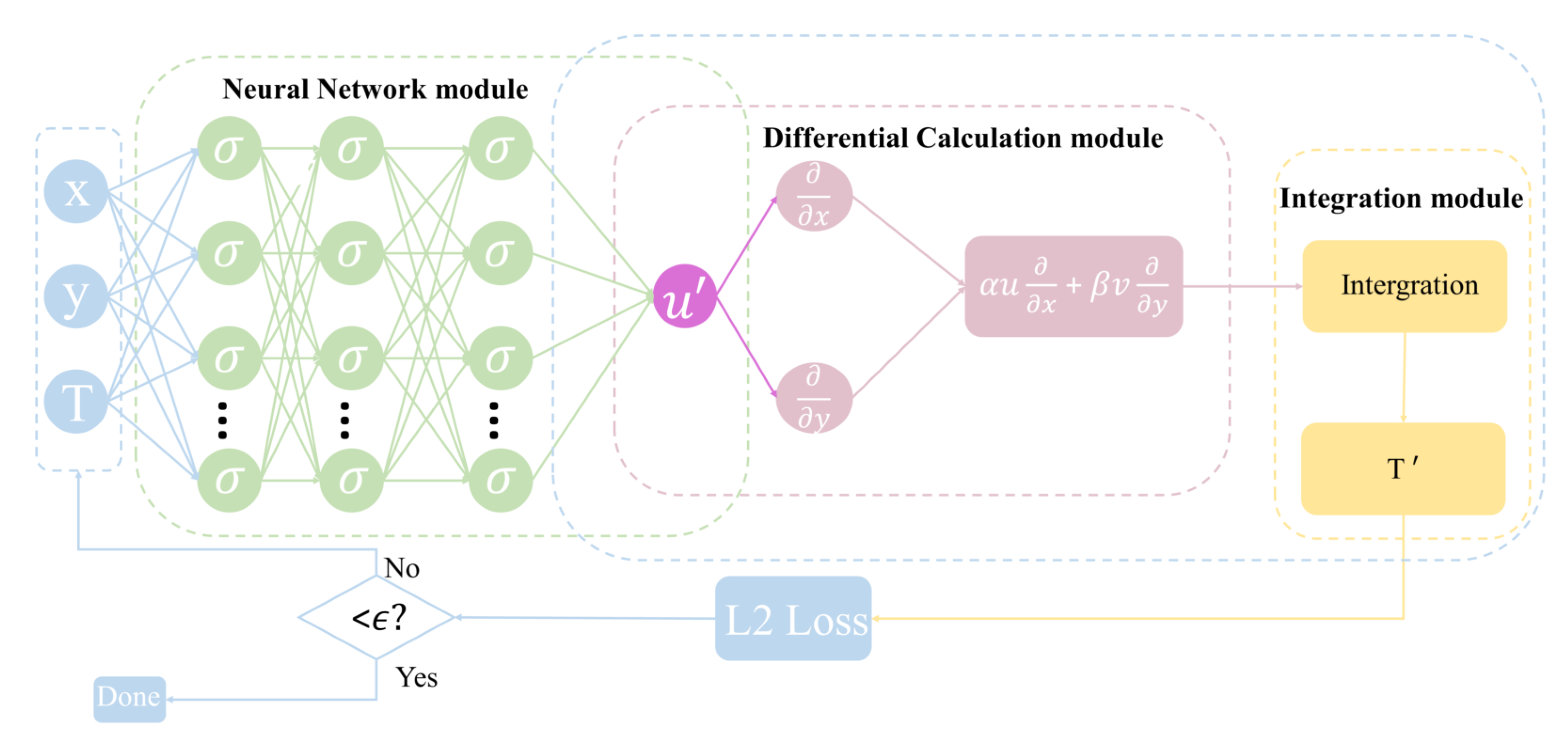
Figure 1. The framework of our proposed STPDE-NET.
Remotesensing 15 03498 g001
Figure 2. Model applied in the neural network module: 3D-CNN, 3D-ConvLSTM, and Vision Transformer. Reprinted with permission from Refs. [13,46,47,48,49].
Remotesensing 15 03498 g002
Figure 3. Overview of our proposed STPDE-NET used to predict the daily SST. Three basic strategies are used: a CNN_based model, ConvLSTM_based model, and ViT_based model with various model parameters. The 11 marine variables and coordinate information are from time ϵ 6 day to time ϵ 0 days, between 5°S to 5°N and 170°W to 120°W. The seven-day-covered SST value from time ϵ + 1 day to ϵ + 10 day is applied as an output. The blue rectangular block represents the research area of this paper. M is the number of feature maps, and the global map was designed using Matplotlib. The numbers next to each coordinate axis (10, 50, 120, 360) represent the corresponding longitude and latitude information.
Remotesensing 15 03498 g003
Figure 4. RMSE of SST prediction using 10 years of data for different prediction horizons (1–10 days).
Remotesensing 15 03498 g004
Figure 5. Five-day lead RMSE for SST prediction (2010–2019).
Remotesensing 15 03498 g005
Figure 6. Ten-day lead RMSE for SST prediction (2010–2019).
Remotesensing 15 03498 g006
Figure 7. Statistical significance error between SST generated based on the HYCOM numerical model [8] and SST from reanalysis data.
Remotesensing 15 03498 g007
Figure 8. Effect analysis of the mixed layer temperature tendency term (Tend), the net surface heat flux term ( Q n e t ), the individual zonal, meridional, vertical advection terms (ZAdv, MAdv, and VAdv) averaged over the Western Pacific Ocean (5°S–5°N, 170°W–120°W using the above three models).
Remotesensing 15 03498 g008
Table 1. Input variables for sea surface temperature modelling.
Input VariablesData Source
1Downward Longwave Radiation (in W / m 2 )ERA5
2Upward Longwave Radiation (in W / m 2 )ERA5
3Downward Shortwave Radiation (in W / m 2 )ERA5
4Upward Shortwave Radiation (in W / m 2 )ERA5
5Latent Heat (in W / m 2 )ERA5
6Sensible Heat (in W / m 2 )ERA5
7Sea Surface Temperature (in  ° C )NOAA and CMEMS
8Sea Surface Temperature at 108 m (in ° C )CMEMS
9Momentum Flux-u-Component (in m / s )CMEMS
10Momentum Flux-v-Component (in m / s )CMEMS
11Vertical Ocean Current Velocity at 108 m (in m / s )CMEMS
12Mixed Layer Thickness (in m )CMEMS
13Longitude (-)all data source
14Latitude (-)all data source
Table 2. Improved performance (mean ± std) of the empirical equation using three algorithms (compared with the finite difference method) in predicting the SST RMSE using different numbers of datasets (1–10 years).
Models1 Day5 Day10 Day
Number of sample: 10 year
STPDE-NET-118.56 ± 0.15%13.15 ± 0.12%10.52 ± 0.08%
STPDE-NET-214.99 ± 1.60%13.69 ± 1.47%21.01 ± 1.39%
STPDE-NET-33.36% ± 2.40%5.07% ± 1.80%4.44% ± 2.51%
Number of sample: 9 year
STPDE-NET-118.88 ± 0.85%18.12% ± 0.28%11.11 ± 0.14%
STPDE-NET-215.27 ± 3.04%20.47 ± 1.78%21.90 ± 2.40%
STPDE-NET-33.83 ± 1.25%11.23 ± 0.46%6.67 ± 1.30%
Number of sample: 8 year
STPDE-NET-118.42 ± 0.00%13.47 ± 0.60%10.60% ± 0.40%
STPDE-NET-29.26 ± 2.29%10.97 ± 3.09%15.91 ± 2.44%
STPDE-NET-35.21 ± 0.73%6.00 ± 0.82%7.34 ± 0.84%
Number of sample: 7 year
STPDE-NET-118.23 ± 0.19%13.28 ± 0.00%10.75 ± 0.00%
STPDE-NET-214.70 ± 0.84%11.41 ± 0.85%13.87% ± 2.74%
STPDE-NET-32.15 ± 2.19%−10.4 ± 12.39%3.15 ± 3.47%
Number of sample: 6 year
STPDE-NET-118.87 ± 1.27%13.85 ± 0.30%11.30% ± 0.35%
STPDE-NET-217.52 ± 1.44%12.55 ± 1.80%15.48 ± 2.92%
STPDE-NET-33.72 ± 2.92%4.94 ± 1.01%6.27 ± 2.36%
Number of sample: 5 year
STPDE-NET-118.78 ± 1.16%14.55 ± 0.84%12.20 ± 0.51%
STPDE-NET-216.41 ± 4.11%12.39 ± 2.96%10.31 ± 2.16%
STPDE-NET-33.76 ± 0.61%5.36 ± 0.37%6.13 ± 0.07%
Number of sample: 4 year
STPDE-NET-120.22 ± 1.18%15.27 ± 0.69%12.68 ± 0.49%
STPDE-NET-218.47 ± 1.44%15.48 ± 0.61%15.02 ± 3.08%
STPDE-NET-33.83 ± 2.89%4.94 ± 0.70%6.18 ± 0.62%
Number of sample: 3 year
STPDE-NET-120.54 ± 1.08%14.98 ± 0.66%12.58 ± 0.51%
STPDE-NET-221.46 ± 0.97%16.80 ± 0.55%13.85 ± 5.31%
STPDE-NET-34.87 ± 0.54%4.82 ± 1.07%6.43 ± 0.46%
Number of sample: 2 year
STPDE-NET-119.53 ± 0.19%15.69 ± 0.13%12.86 ± 0.00%
STPDE-NET-213.77 ± 7.79%14.09 ± 2.86%13.37 ± 3.81%
STPDE-NET-36.33 ± 1.59%6.90 ± 0.66%6.79 ± 0.11%
Number of sample: 1 year
STPDE-NET-117.88 ± 0.11%11.93 ± 0.14%9.06 ± 0.00%
STPDE-NET-213.97 ± 8.19%9.48 ± 1.07%6.26 ± 1.30%
STPDE-NET-31.31 ± 0.35%2.29 ± 0.51%3.47 ± 0.38%
Disclaimer/Publisher’s Note: The statements, opinions and data contained in all publications are solely those of the individual author(s) and contributor(s) and not of MDPI and/or the editor(s). MDPI and/or the editor(s) disclaim responsibility for any injury to people or property resulting from any ideas, methods, instructions or products referred to in the content.