Abstract
The main scope of the study is to evaluate the prognostic accuracy of a one-dimensional convolutional neural network model (1D-CNN), in flood susceptibility assessment, in a selected test site on the island of Euboea, Greece. Logistic regression (LR), Naïve Bayes (NB), gradient boosting (GB), and a deep learning neural network (DLNN) model are the benchmark models used to compare their performance with that of a 1D-CNN model. Remote sensing (RS) techniques are used to collect the necessary flood related data, whereas thirteen flash-flood-related variables were used as predictive variables, such as elevation, slope, plan curvature, profile curvature, topographic wetness index, lithology, silt content, sand content, clay content, distance to faults, and distance to river network. The Weight of Evidence method was applied to calculate the correlation among the flood-related variables and to assign a weight value to each variable class. Regression analysis and multi-collinearity analysis were used to assess collinearity among the flood-related variables, whereas the Shapley Additive explanations method was used to rank the features by importance. The evaluation process involved estimating the predictive ability of all models via classification accuracy, sensitivity, specificity, and area under the success and predictive rate curves (AUC). The outcomes of the analysis confirmed that the 1D-CNN provided a higher accuracy (0.924), followed by LR (0.904) and DLNN (0.899). Overall, 1D-CNNs can be useful tools for analyzing flood susceptibility using remote sensing data, with high accuracy predictions.
1. Introduction
Flood phenomena are considered one of the most devastating natural disasters. In 2022, floods were the dominant natural hazards worldwide, with 176 occurrences, which is above the average number of 168 annual flood occurrences recorded in 2002–2021, followed by storms (108) and earthquakes (31). The flood events that occurred in 2022 resulted in the loss of 7954 lives worldwide and caused economic losses amounting to USD 44.9 billion [1]. Flood phenomena occur when the hydrographic network cannot drain the volume of water that flows, usually during heavy rain events, resulting in water overflowing and occupying ephemeral parts of land. The amount and intensity of precipitation, the permeability and infiltration capacity of the geological formations, as well as the morphological characteristics of the basin are considered the three main natural components that control flood phenomena. The causes of flood phenomena can be distinguished into natural and artificial. Natural causes involve heavy rainfall or the melting of snow, which result in the overflowing of rivers and lakes in lowland areas, the transport of water from upstream areas and non-permanent watercourses, and also the increased runoff of water due to the uplifting of groundwater table. The effects of tidal phenomena, heavy storms, and tsunami waves belong to the natural causes that affect the intensity and extent of floods, particularly in coastal areas. Artificial causes include the failure of hydraulic works, such as dams, dykes, and aqueducts, and the under-dimensioning or poor operation (e.g., of solid waste) of the rainwater drainage network. Most of the flood phenomena that occur in Greece are characterized as flash floods, i.e., a type of flooding characterized by high velocities and strong erosive characteristics.
According to [2], in Greece, a considerable number of flood events have occurred. From 2000 to 2020, more than 380 flood episodes were recorded, causing significant social and economic consequences. These include the loss of 132 lives (with 38 fatalities occurring in the Attica Prefecture), damage and destruction of infrastructure, transportation disruptions, and more. Most floods occur in eastern Greece, despite western Greece experiencing higher rainfall amounts. However, floods in western Greece typically have fewer casualties. These events tend to happen in areas located within a short distance from the coast (less than 5 km) and at low altitudes (less than 50 m). The average slope in these regions is around 10–15%, and the basins affected are generally smaller than 100 km2 [3].
Natural disasters, such as floods, require an organized society to ensure safety conditions for its citizens and the preservation of the environment. To mitigate the adverse impacts of such catastrophic events, significant efforts are dedicated to prediction and early prevention. Rather than solely focusing on post-event damage assessment, flood management endeavors prioritize the assessment of susceptibility and vulnerability in flood-prone areas [4]. In flood hazard and risk assessment surveys, susceptibility mapping is a valuable method for identifying areas prone to flooding. Unlike other approaches, susceptibility mapping focuses on identifying flood-prone areas without explicitly considering triggering events or temporal variables. Recently, there has been a growing adoption of data-driven methods, particularly machine learning (ML) models, in environmental studies. This is primarily due to the rapid advancement in technology in both hardware and software. Technological progress has enabled the development and implementation of innovative and computationally demanding algorithms. Furthermore, the availability of large datasets from various sources has facilitated the application of ML techniques. In flood susceptibility assessments, ML techniques are employed in an iterative process to minimize prediction errors, primarily through supervised learning. The key objective of utilizing ML in flood susceptibility assessments is to uncover hidden patterns in flood-related data that might contribute to the occurrence of floods [5,6]. By leveraging the power of ML algorithms, patterns and relationships within the data can be identified, leading to more accurate predictions of flood susceptibility. ML models can analyze various factors such as topography, hydrological characteristics, land use, and historical flood events to identify the key variables that contribute to flood occurrence. Logistic regression, fuzzy logic, Naïve Bayes, artificial neural networks, support vector machine, neuro-fuzzy, adaptive neuro-fuzzy inference system, decision trees, and random forest are the most widely used machine learning methods [5,6,7,8,9,10,11]. Deep learning (DL) methods, i.e., a subtopic of machine learning algorithms, are the “hot” topic for researchers and are used in various applications for supervised or unsupervised methods, classification, and regression tasks. They are rather efficient and useful when the dataset size is very large [12,13]. Apart from flood-related assessments, these techniques have been applied in other natural hazards, such as landslides, debris flows, erosion, subsidence, forest fires, etc. [14,15,16,17,18,19]. Their wide use is related to their capability to model hidden and unknown complex relations that may appear among data by exploiting multiple layers of nonlinear information, most commonly using a multilayer neural network (MLP-NN), which is much more efficient than conventional ML methods [20]. Supervised DL models involve the standard multilayer perceptron neural network that has more than two or more hidden layers, convolutional neural networks (CNN), recurrent neural networks (RNN), and transformer networks. Unsupervised DL models that are not pre-trained involve self-organizing maps (SOM), Boltzmann machines, and autoencoders.
Along with standard DL neural network models, CNNs are the most widely used models in DL applications. Their popularity is mainly attributed to the ability to automatically detect the important features in a dataset [21]. The implementation of CNN involves the analysis of very-high-resolution remote sensing images for classification and segmentation processes [22], semantic segmentation [23], and object detection and recognition [24,25]. In the scientific literature, one can find the implementation of CNNs in flood, landslide, debris flow, and forest fire susceptibility mapping studies, and the authors of the studies report CNNs’ higher predictive performance when compared to conventional ML algorithms [12,13,26,27,28,29,30,31]. The architecture of a CNN includes the following layers: input, hidden, convolutional, max pooling, fully connected, and output [32], and in most cases the presence of training datasets from known recorded cases [24]. There are many known architectures of CNNs that have been developed for various image recognition tasks, such as: LeNet-5, AlexNet, VGGNet, ResNet, and InceptionNet [33]. Each architecture has its own strengths and weaknesses, and the selection of architecture depends on the specific image recognition task and the size of the dataset, and thus most researchers develop their own models. This is because the architecture of a CNN can have a significant impact on its performance, and developing a customized architecture that is tailored to a specific task can lead to better results. There are different types of CNN models in respect to the dimensionality of the input data, like 1D-CNNs, which handle one-dimensional data; 2D-CNNs, designed for two-dimensional data; and 3D-CNNs, designed for three-dimensional data. While the basic principles of CNN models remain the same across all three types, the architecture and design of 1D, 2D, and 3D CNNs can differ significantly due to the differences in the input data.
Customized or known CNN architecture models have been used in flood assessments. For example, Zhao et al. [34] introduced a CNN model to assess flood susceptibility for the Dahongmen urban catchment in Beijing, China, evaluating its validity and high predictive performance. In the study, SCNN and LeNet-5 models were implemented and compared with the performance of a SVM and a RF model using a point-based, an array-based, and an imaged-based input strategy. The fixed-architecture LeNet-5 produced satisfactory results. Wang et al. [12] proposed three CNN models, 1D-CNN, 2D-CNN, and 3D-CNN, in flood susceptibility mapping in the county of Shangyou, China. The outcomes of the study suggested that all the CNN-based methods produced reliable and accurate flood susceptibility maps, surpassing in performance conventional machine learning models. Ullah et al. [35] proposed a multi-hazard susceptibility mapping approach for the prediction of the probability of the occurrence of flash floods, debris flows, and landslides using CNN. The authors report that CNN outperformed the conventional machine learning algorithms, LR and k-NN.
Remotely sensed data play a crucial role in flood susceptibility mapping and can provide valuable information about the landscape and environmental factors that contribute to flood occurrences. Remote sensing techniques, such as satellite imagery and aerial photography, allow for the collection of high-resolution data on various flood-related variables, including land cover, topography, hydrological characteristics, and historical flood events [22,34]. The integration of these data sources with advanced deep learning algorithms can enhance the understanding and prediction of flood events, ultimately leading to more effective flood management and mitigation strategies.
In this context, the present study utilizes a 1D-CNN model to evaluate and produce a flash flood susceptibility map, assuming a one-dimensional input vector which describes the corresponding flood-related variables, whereas satellite images and cartographic flood-related products were used to extract flood and non-flood areas. The methodology introduced in the present study was developed to present intelligent ways of utilizing DL algorithms used in flash flood susceptibility assessments and compare their performance against conventional ML models. R packages and python scripts in R and Python Shell and ArcGIS 10.5.1 [36] were used for compiling the spatial data and generating the flash flood susceptibility maps. The learning and predictive performance of the developed methodology along with the performance of the benchmark models were tested in an area located in the island of Euboea, Greece.
2. Study Area
The island of Euboea has an area of 3684 km2, with a population of 191,206 (population density 54/km2) [37]. The study area covers an area of 654 km2, which is delimited by two major and three minor water basins where the Lilas and Messapios Rivers and the streams of Politika, Poros, and Mantania flow (Figure 1). The area is characterized by gentle slopes apart from the high-altitude areas. Approximately 38% of the study area is characterized as open slopes, 21% as plains, and 18% as upper slopes. The lithological units that cover the area include Quaternary and Neogene formations, carbonate rocks, schist, flyschoid formations, and magmatic/volcanic rocks. In detail, the area is covered by recent and old quaternary deposits, Neogene formations, mainly marly limestone and conglomerate, flysch formations, limestone, shale and phyllites, ophiolites, flint, and shaly siltstone [38].
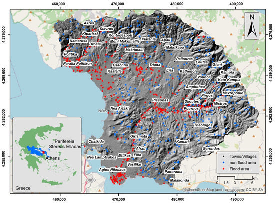
Figure 1.
Study area.
Concerning the climate of the study area, it is characterized as Mediterranean. The Mediterranean climate is characterized by dry summers and mild, wet winters and a distinct seasonal pattern of rainfall, influencing various aspects of the natural environment, including vegetation, agriculture, and water resources management. During the summer, Mediterranean climates generally have a pronounced dry period, with little to no rainfall, while rainfall is more possible in the winter [39]. In the study area, the mean annual rainfall varies depending on the location. In lowland and coastline areas, the average annual rainfall is around 450 mm, while in high-altitude areas, it increases to approximately 550 mm. The distribution of rainfall throughout the year also exhibits seasonal variations. The period from November to January typically experiences the highest precipitation amounts, indicating the peak of the rainy season. During this time, the region receives the most substantial portion of its annual rainfall. On the other hand, the months from July to August are characterized by the lowest precipitation amounts, reflecting the drier summer season [40].
The wider study area has a history of flood events that have caused significant damage to various aspects of the region, including agricultural land, infrastructure, buildings, and the coastal area. These flood events have occurred predominantly between September and December. The recent extreme rainfall event of August 2020 resulted in severe flood phenomena and the unfortunate loss of eight citizens in the areas of Psachna, Politika, Lefkanti, Vasiliko, and Bourtzi, highlighting the vulnerability of the region to heavy rainfall and subsequent flooding [41]. In the Messapios river basin, the occurrence of a forest fire in August 2019 near the Psachna settlement had a rather minor influence on the severity of the flood phenomenon [41]. Figure 2 shows the devastating effects of the flood phenomenon, which included huge volumes of debris materials, tree trunks, and large branches, and severe damage to roads, infrastructure, and buildings. The severity of the consequences of the flood event and the frequent recurrence of the phenomena in the specific area made it suitable for the implementation of a newly developed flood prediction methodology to evaluate its efficiency and predictive performance.
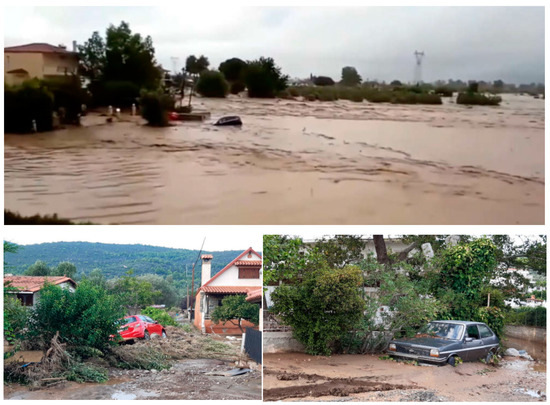
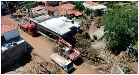
Figure 2.
Flooded areas and debris flow [41].
3. Materials and Methods
The methodology developed during the present study follows a 5-phase process, which involves: (i) the construction a flash flood and non-flash-flood inventory, (ii) data selection, classification, weighting, and normalization, (iii) Pearson’s correlation, multi-collinearity, and importance analysis, (iv), application of a 1D-CNN model and construction of the flood susceptibility maps, and (v) estimation of the prediction ability of the 1D-CNN model and comparison of its performance with other benchmark machine learning algorithms. The successful completion of each phase has a significant impact on the final deliverable. The three first phases (i, ii, and iii) are preprocessing phases that ensure the overall quantity and quality of the training data. The process of constructing the inventory database; selecting, classifying, and weighting the appropriate flood-related parameters; and estimating their dependency, correlation, and predictive power are the essential actions. The last two phases involve the implementation and validation of the DL and conventional ML models, and the generation of the flood susceptibility map. Figure 3 depicts the flowchart of the five-phase methodology, providing a visual representation of the sequential process followed to develop the flood prediction framework.
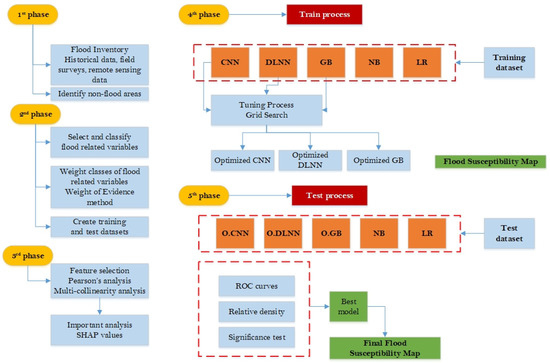
Figure 3.
Flowchart of the followed methodology.
3.1. First Phase—Inventory Database
The first phase involved the construction of the flash flood and non-flash flood inventory. The data were obtained from previous studies, satellite image processing, and cartographic products available from the Greek Ministry of Environment and Energy (GMEE) and the European Environment Agency (EEA) [41,42,43,44]. The satellite images were available from the European Space Agency’s Copernicus Program and the Sentinels Scientific Data Hub (SSDH). The Copernicus Sentinel satellites, particularly Sentinel-2, capture imagery in multiple spectral bands, including the visible, near-infrared, and shortwave infrared ranges. These bands provide valuable information about the land cover, vegetation health, and water bodies, and in our case, facilitate the accurate identification and delineation of flooded areas. The SSDH provide high-resolution imagery with pixel sizes as small as 10 m. This level of detail allows for the precise identification and mapping of flooded areas, including smaller water bodies and localized flood events. The Copernicus Program operates a constellation of satellites that cover the entire globe systematically with Sentinel-2 capturing imagery every 5 days following an open data policy, making its products available to the public. Two satellite images, before and after the flood events that occurred in August 2020 (3 August 2020 and 13 August 2020, respectively) were assessed to identify the flooded areas. The flooded area was identified based on the Difference of Normalized Difference Water Indices (DNDWI) using the green (B03) and near-infrared bands (B08) to highlight water bodies of Sentinel-2 detectors as proposed by [45] (Equation (1)). Band 3 has a resolution of 10 m/pixel, a central wavelength of 560 nm, and a bandwidth of 35 nm, whereas Band 8 has a resolution of 10 m/pixel, a central wavelength of 842 nm, and a bandwidth of 115 nm. NDWI expresses the ratio of the difference in the sum of the intensities of radiation at near-infrared and green wavelengths [46]:
where DNDWI represents the Difference of Normalized Difference Water Index, B03A and B03B the green band, and B08A and B08B the near-infrared (NIR) band, for the two time periods after (A) and before (B) the flood event.
A total of 400 points from the flooded areas were randomly created by using the geo-processing tool Create Random Points, included in the Data Management Tool of the ArcGIS platform [36], which along with 13 past flood events generated the flood inventory database. The non-flooded locations were generated from the area outside the areas of Potential Significant Flood Risk (APSFR). The APSFR areas have been developed following the Directive 2007/60 of the European Union and the potential flood area (100-year return period) by the Ministry of Environment and Energy [44]. The potential flood-prone area extent delineates the area that is flooded once every 100 years assuming that flooding is unrestricted, with the potential flood-prone area comprised of the river channel and the floodplain. Figure 4a illustrates the outcome of the extraction process from the Copernicus Sentinel-2 product, whereas Figure 4b shows the APSFR and potential flooded areas.
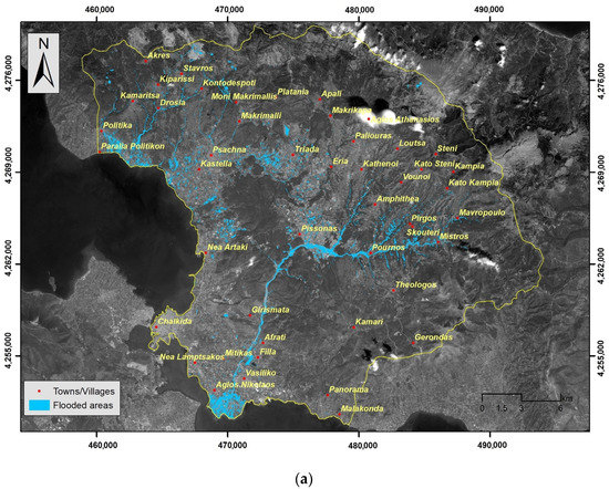
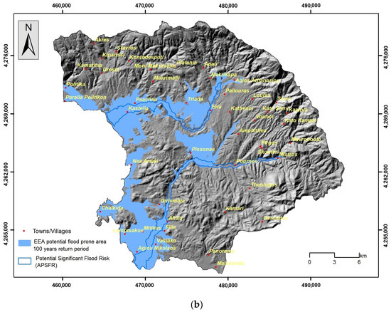
Figure 4.
(a) Flash flood area—August 2020. (b) Potential flood areas (100-year return period)— potential significant flood risk.
3.2. Second Phase
The second phase involved the selection of the appropriate flood-related variables, the classification and weighting process, and the construction of the training and testing database. The selection of the flood-related variables was based on the knowledge gained from the study of previous reports with similar characteristics, the scientific literature, and data availability. The morphological, lithological, and hydrological characteristics; the soil cover and land use cover maps; and the climate variables were derived from various sources. Thirteen factors were considered, namely: elevation, slope, profile curvature, plan curvature, Topographic Wetness Index (TWI), Topographic Position Index (TPI), distance from river network, lithology, soil content (percentage of silt, sand, and clay content), land use cover [47], and rainfall (Modified Fournier Index). The classification process involved transforming the continuous flash-flood-related variables into variables with discrete classes. Lithology and land cover did not undergo any classification process since the raw data appeared with discrete classes.
The weighting process involved the implementation of the Weight of Evidence (WofE) method, which is a probability-data-driven approach [48,49,50]. The WofE method can estimate the relation concerning the spatial distribution of the flooded areas and the spatial distribution of the flood-related variables, expressed by the magnitude of contrast (C). C is a measure that is estimated by the difference in positive spatial correlation between the flood-related variables and the flood locations (W+) and analogous negative spatial correlation (W−). A positive C implies a positive correlation, whereas a negative C implies a negative spatial association [51] (Equation (2)).
is the prior posterior probability that a flood event (F) will occur under the presence of an evidence A or the absence of an evidence . The C value expresses the influence that each flood-related variable has on the occurrence and evolution of a flood event.
3.3. Flood-Related Variables
The geomorphological parameters such as elevation, slope, plan curvature, profile curvature, TWI, and TPI were obtained by applying geoprocessing spatial tools from the ArcGIS suite using data from the Alaska Satellite Facility (ASF), which provides a PALSAR Phased Array type L-band DEM (Digital Elevation Model) with a resolution of 12.5 m (https://asf.alaska.edu/data-sets/sar-data-sets/alos-palsar/ (accessed on 14 November 2022) (Table 1) [52]. Lithological cover and distance from the river network were obtained from the geological (Euboea, scale 1:200,000) and topographic map sheets of the wider research area (Psachna, Chalkida sheet, scale 1:50,000) [38]. The MFI was produced using data from the WorldClim v.2.1 database [53]. The sand, silt, and clay cover were obtained from the LUCAS topsoil database [54], whereas the CORINE Land Cover (CLC) of the year 2018 provided by the Copernicus Land Monitoring Service was used for extracting the land use cover [47]. All flood-related parameters were transformed into raster format of 12.5 m by 12.5 m grid cell after applying resampling and downscaling methods where necessary [36].

Table 1.
Flood-related variables, source, and influence on flood occurrence.
Elevation has a significant influence on flood occurrence; higher elevation areas show fewer chances of flooding, and vice versa [8,55,56]. The elevation was classified into nine classes (<40 m, 41–80 m, 81–120 m, 121–160 m, 161–200 m, 201–240 m, 241–280 m, 281–320 m, and >321 m) (Figure 5a). Steepness is another controlling factor in water flow. Thus, areas of lower slope angles show an increased probability of water appearance, which may allow increased infiltration rates and lower surface runoff velocities and could be characterized as more susceptible to floods [55,57,58]. The slope parameter was classified into 5 classes (<5°, 6°–10°, 11°–20°, 21°–30°, and >31°) (Figure 5b). The plan and profile curvature variable influence the manifestation of floods in water basins [59]; positive values indicate a convex surface, while a negative value corresponds to a concave surface [56]. Plan curvature corresponds to the surface that is perpendicular to the direction of the maximum slope and influences the magnitude of convergence or divergence of a fluid flow across a surface. Profile curvature corresponds to the surface that is parallel to the slope surface and influences the acceleration or deceleration of fluid flow across a surface [36]. Three classes were created in this regard (<−0.05, −0.04–0.05, and >0.06) (Figure 6a,b). The TWI is another factor responsible for flood occurrence, which can indicate areas that, from a topographic context, are prone to concentrate water [56,60,61]. Here, the TWI was reclassified into 5 classes (<6.02, 6.03–7.31, 7.32–8.94, 8.95–11.33, and >11.34) based on the Natural Breaks (Jenks) classification method [36] (Figure 7a). The TPI is the difference between the elevation value of a surface and the mean elevation value of a specified neighborhood around that surface, and it is used to identify topographic features such as a hilltops, valley bottoms, exposed ridges, flat plains, and upper or lower slopes [62,63,64]. In general, steep and high-elevation areas are less likely to experience flood events than low-relief areas [65]. The TPI was reclassified into 5 classes (<−18.30, −18.29–5.97, −5.96–3.63, 3.64–15.96, and >15.97) based on the Natural Breaks (Jenks) classification method [36] (Figure 7b). Lithology is another important flood-related variable related to the infiltration rate and the water flow [20,66]. In general, geological formations of low permeability are more susceptible to flooding. The research area is covered by recent and old quaternary deposits, Neogene formations, mainly marly limestone and conglomerate, flysch formations, limestone, shale and phyllites, ophiolites, flint, and shaly siltstone (Figure 8a). Land use cover affects evaporation, infiltration, and runoff [57]. Regions which are covered by farmlands and green land show lower susceptibility to flooding compared to urban areas, which are covered by impermeable surfaces which favor surface runoff [66] (Figure 8b). Soil cover is another critical factor responsible for the generation of floods. Soils that are characterized by a high percentage of sand absorb water at a higher rate and more likely prevent surface runoff, whereas soils characterized by a high percentage of clay are less porous; they store water and are more prone to flooding [67,68]. The absorbance ability of the topsoil, which depends on the percentage of sand, clay, and silt, was considered in the analysis [54] (Figure 9a,b and Figure 10a). The distance from the river network affects the extent of flooding [66] since the surfaces’ water storages are related to floods [56]. The areas which are close to the hydrographic network appear to be more susceptible to flood occurrence [59]. The distance to river network was classified into 4 classes (50 m, 51–100 m, 101–200 m, and >201 m) (Figure 10b). Rainfall is a major contributor in flood occurrence; intense and short rainstorms favor the generation of flash floods [20]. Here, the MFI was introduced to include the rainfall influence in the flood susceptibility analysis. Twelve (12) GEOTIFF files concerning mean monthly rainfall values were obtained from the WorldClim v.2.1 repository and clipped to the study area extent, whereas a resampling technique based on inverse-distance weighting was applied [53]. Rainfall aggressiveness is a function of the interactions between the height and duration of rainfall events. The Modified Fournier Index (MFI), which represents the ratio between average monthly rainfall and average annual rainfall, is a strong indicator of rainfall aggressiveness and potential flash-flood-related events [69,70]. The MFI variable was reclassified into 3 classes which are shaped by the Natural Break (Jenks) classification scheme (<55, 56–65, and >66) [36], with higher values indicating flood-prone areas (Figure 11).
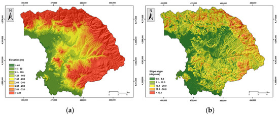
Figure 5.
(a) Elevation, (b) slope angle.
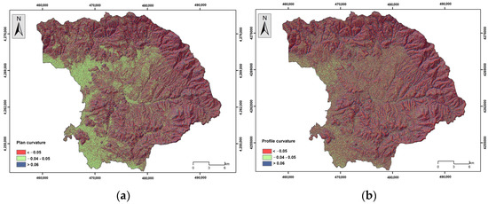
Figure 6.
(a) Plan curvature, (b) profile curvature.
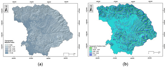
Figure 7.
(a) Topographic Wetness Index, (b) Topographic Position Index.
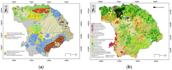
Figure 8.
(a) Lithology, (b) land cover.
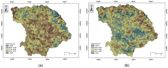
Figure 9.
(a) Sand cover, (b) clay cover.
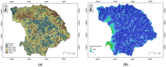
Figure 10.
(a) Silt cover, (b) distance from river network.
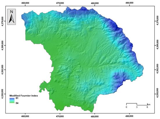
Figure 11.
Modified Fournier Index.
3.4. Third Phase—Pearson’s Correlation—Multi-Collinearity Analysis and Importance Analysis
3.4.1. Pearson’s Correlation
The third phase involves the estimation of the Pearson correlation coefficient. Also known as Pearson’s r, it is a statistical measure which expresses the linear correlation between two datasets. It is commonly used to assess the degree to which two variables are related and to determine the extent to which changes in one variable are associated with changes in the other. The output of the analysis provides values that range between −1 and 1. A highly linear correlation is present when values are equal to or greater than 0.7, a significant linear correlation is between 0.5 and 0.7, a low linear correlation is between 0.3 and 0.5, and no linear correlation exists with values lower than 0.3.
3.4.2. Multi-Collinearity Analysis
In classification or regression problems, the independent/explanatory variables should not be correlated. In the case in which the variables appear correlated, this correlation affects the ability to evaluate their individual effects on the variable that must be estimated, a problem known as multi-collinearity [3]. During the multi-collinearity analysis, two metrics, the Variance Inflation Factor (VIF) and the tolerance index (TOL), are calculated, with the presence of severe multi-collinearity in databases that have a VIF index higher than 5 and a TOL index lower than 0.1.
3.4.3. Importance Ranking—Shapley Additive Explanations—SHAP
Shapley Additive Explanations (SHAP) is a powerful method for importance ranking and the interpretation of machine learning models. The SHAP method is based on cooperative game theory and provides a unified framework to quantify the contribution of each feature towards the prediction of a model. It was proposed by Lloyd Shapley [71]. Shapley (SHAP) has gained popularity due to its ability to provide interpretable explanations in a model-agnostic manner, making it applicable to a wide range of machine learning algorithms and domains [72].
A Shapley value expresses the average marginal contribution of an instance of a feature among all possible combinations. The SHAP value ϕi(f,x) is a numerical value that describes the influence of the ith factor in the model prediction f, and x is the given input. Factors with large absolute Shapley values are important. SHAP is also included in the R xgboost package [73]. The absolute Shapley values per factors across the data are based on the following, Equation (3):
3.5. Fourth Phase—Applying Deep Learning Models and Benchmark Machine Learning Models and Constructing the Flood Susceptibility Maps
3.5.1. Convolutional Neural Network CNN
CNNs are inspired by biological brain activities, and in particular, the section which is responsible for the perception of vision, with the theoretical models proposed by Hubel and Wiesel back in 1959 [Hubel and Wiesel, 1959] [74]. The neurons in the visual cortex are arranged in a hierarchical manner, with each layer processing increasingly complex features. Similarly, CNNs consist of multiple layers of artificial neurons, with each layer learning and extracting different features from the input data. The convolutional layers in CNNs use filters to perform local operations on the input data, like how the receptive fields of neurons in the visual cortex respond to local regions of the visual field. A CNN architecture typically consists of three layers: convolutional, pooling, and fully connected (Figure 12).
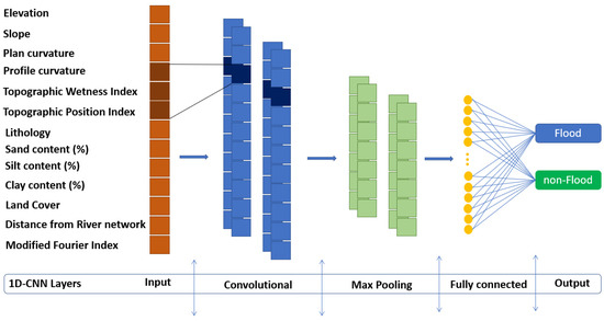
Figure 12.
Architecture of a 1D convolutional neural network.
CNNs have been used to deal with these complex problems, as they can extract and learn localized features. They have a hidden layer with one or more convolutional layers, pooling layers, and fully connected layers, as shown in Figure 12. Several filters have been used in the convolutional layers to divide the input data into small dimensional parts. Pooling layers are robust in dealing with distortion and noise by reducing the number of factor maps. Finally, the fully linked layer connects all neurons to the neurons in the previous layer to integrate the data with group differentiation in the convolutional and pooling layers. In the CNN technique, the convolutional layer applies a set of convolution kernels to learn an effective representation from the input data. If we have an input, the feature vectors are V, which represents V1 to Vn (Equation (4)):
If the kernels (k) are in the convolutional layer and the jth kernel has the weight (Wj) and bias (bj), then the output (Cj) of the convolutional method can be calculated using the following equation (Equation (5)):
where (f) is the nonlinear activation operation and (∗) is the convolution operator.
To reduce the size of the feature vector and avoid the overfitting issue, the pooling layer (max-pooling) that follows the convolution layer was used. By applying the max pooling method, the length of the feature vectors is reduced, and the depth remains unaltered. This step is followed by fully concatenated layers that detect the extracted feature vectors. Finally, softmax activation is used to transfer the detected vector into a prediction probability for the corresponding category, which is calculated as follows (Equation (6)):
where m and M represent the predicted class and the number of categories, respectively; Wm and Wn represent the weight vectors; and βm and βn represent the bias vectors.
The model’s accuracy is, in some manner, controlled by the choice in hyperparameters, such as the number of layers and neurons, the batch size and number of epochs, the learning rate, the optimizer, and the activation functions. To capture the high-level features, we used a filter size of 3 × 3 with stride length of 2. The high-level features were aggregated using a max pooling layer, and the activation function used was Rectified Linear Unit (ReLU). The experiments were conducted using the Kaggle platform, choosing the accelerator GPU T4 × 2 NDVIA and 30 GB of RAM.
3.5.2. Benchmark Models
In this phase, a comparison was made with several benchmark models. Specifically, logistic regression (LR), Naïve Bayes (NB), gradient boosting machine (GBM), and deep learning neural network (DLNN) were among the benchmark models.
Logistic Regression (LR)
According to Chau and Chan [75], LR provides the probability of an event to occur over the probability of non-occurrence. In our case, the objective is to identify the relation between the occurrence of a flood event and its dependency on flood-related variables, which is expressed by Equation (7):
where pflood is the probability of a flood.
The pflood ranges from 0 to 1, plotted on an S-shaped curve, whereas the z factor expresses the linear relation of the flood-related variables. LR involves applying an equation to the dataset, like the following (Equation (8)):
where b0 is the intercept, bi is the slope coefficients of the logistic regression model, and xi is the flood-related variables.
z(xi) = b0 + b1×1 + b2×2 + … + bn×n
Gradient Boosting
Gradient boosting (GB) is a powerful supervised machine learning technique that combines multiple weak predictive models to create a stronger and more accurate predictive model, developed by Friedman [78]. It can be used for regression and classification tasks, as it optimizes an objective function by iteratively adding models that focus on the samples where the previous models performed poorly. GB is based on the concept of improving its accuracy on its predecessor gradually by reducing the errors, unlike random forest, in which the learning process—training different decision trees—is parallel. In the case of a GB, the training is based on a sequential manner with each decision tree learning from the errors of the previous ones.
In the case of a flood-related database, , where x = (x1, x2, …, xn) are the flood related-variables and y is the corresponding output, which could be either 0 (non-flood) or 1 (flood). The objective is to reshape the unknown functional dependence with the estimate to minimize a loss function θ(y, f) as follows (Equation (13)):
In classification problems, like ours, the loss function is given as follows (Equation (14)):
where y represents the corresponding label (0 for non-flood or 1 for flood) and p(y) is the predicted probability of the incidence being a flood for all N incidences.
For each flood, the function adds the log probability log(p(y)) to the loss and adds log(1 − p(y)) for each non-flood.
Deep Learning Neural Networks
The final benchmark model during the study was the DLNN model. In a DLNN model, the number of layers and nodes defines the depth of the architecture the model follows, whereas other important elements that must be defined are the activation and transfer functions [79]. In reference to the number of layers and the processing elements that are appropriate for a model, there is no universal rule. With this in mind, a grid search technique was used to indicate the optimized number of hidden layers and nodes. Concerning the activation function, which is used for mapping the nonlinearity relation between inputs and outputs [79,80], the study used the Rectified Linear Unit (ReLu) [81]. In a similar manner to the activation function, the transfer function, which is used to map the nonlinearity of the final hidden and the output layer, the study used the sigmoid activation function. Another important element is the choice in the optimization algorithm which is used to adjust the learning rate. In our case, the Rmsprop technique, a gradient-based optimization technique, was used [82]. Figure 13 illustrates the architecture of the DLNN model used in our study, which consists of thirteen neural networks at the input layer, three hidden layers, and one output layer with two nodes (flood and non-flood).
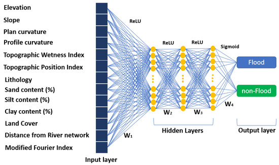
Figure 13.
Deep learning neural network.
3.6. Fifth Phase—Evaluation of the Performance of the Flash Flood Susceptibility Models
The last phase involved the evaluation of the predictive performance of the flood susceptibility model through the receiver operating characteristic curve analysis and calculating the area under the curve value. In addition, the fifth phase involved a pair-wise comparison between the 1D-CNN model and the benchmark models to evaluate the chance that the models produce statistically significant different outcomes, by estimating the p and z values.
4. Results
The correlation between the independent flash-related variables and each other was calculated after applying the Pearson’s method as shown in Figure 14. In most cases, a low linear correlation was identified which indicated that the flash-related variables, which describe the flood phenomena of the research area, are independent of each other. However, a rather high correlation appears between the elevation and the modified Fournier Index, accounting for 0.83. Slightly above 0.50, indicating moderate correlation, appears between sand content cover and silt content cover (0.55) and between elevation and slope (0.53).
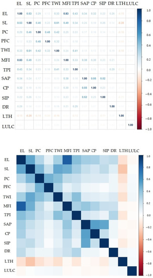
Figure 14.
Pearson’s coefficient. EL: elevation, SL: slope, PFC: profile curvature, PC: plan curvature, TWI: Topographic Wetness Index, TPI: Topographic Position Index, SAP: sand percentage, CP, clay percentage, SIP: silt percentage, DR: distance to rivers, LTH: lithology, LULC: land cover, MFI: Modified Fournier Index.
The multi-collinearity analysis revealed that there is no multi-collinearity issue (Table 2). Therefore, all variables were processed for further analysis. Elevation and MFI were the variables with the lowest Tolerance value (0.2615, 0.2879), which, however, are higher than 0.1, a value which indicates multi-collinearity. They also have higher VIF values (3.8237, 3.4731), values much lower than the value of 10, which indicates multi-collinearity.

Table 2.
Multi-collinearity analysis and importance analysis.
The analysis of variable importance contacted through the SHAP method revealed that within the research area, elevation had the highest SHAP value (0.205), followed by distance from river network (0.120), land cover (0.106), and slope angle (0.067). The summary plot combines feature importance with feature effects (Figure 15 and Figure 16).
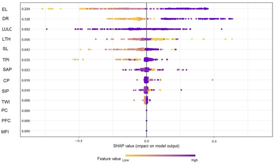
Figure 15.
SHAP values. EL: elevation, SL: slope, PFC: profile curvature, PC: plan curvature, TWI: Topographic Wetness Index, TPI: Topographic Position Index, SAP: sand percentage, CP, clay percentage, SIP: silt percentage, DR: distance to rivers, LTH: lithology, LULC: land cover, MFI: Modified Fournier Index.
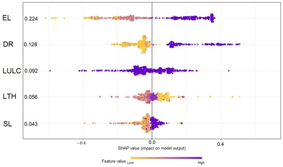
Figure 16.
SHAP values. EL: elevation, SL: slope, DR: distance to rivers, LTH: lithology, LULC: land cover.
Elevation is the variable identified as the variable with the highest impact on the predictions. The Shapley values of elevation are very high or very low. Distance to rivers also seems to have an impact on the predictions, and the rest of the variables are characterized by a lower impact.
For the GB, DLLN, and 1D-CNN models, all the hyperparameter settings were optimized during a training phase using the trial-and-error method [26] (Table 3).

Table 3.
Optimized hyper parameters for GB, DLLN, and 1D-CNN models.
Figure 17, Figure 18, Figure 19, Figure 20 and Figure 21 illustrate the products from the LR, NB, GB, DLNN, and 1D-CNN models’ flood probability/susceptibility maps. All models estimate the probability of flood occurrence and were classified into a five-level probability scheme (<0.25, 0.26–0.50, 0.51–0.75, 0.76–0.90, and >0.91) that corresponds to similar five-level susceptibility characterization (very low susceptibility, low susceptibility, moderate susceptibility, high susceptibility, and very high susceptibility). A rather similar spatial distribution of the flood susceptibility zones was observed, which follows the spatial distribution of elevation and the river network. This has already been identified during the importance analysis, expressed by the SHAP values, where elevation and distance from the river network had the highest values. However, in more detail, there are several differences concerning the coverage of each susceptibility zone among the models. In general, most historical flood incidences are within the high and very high susceptibility zones. Table 4 provides the relative density of flood occurrence in each susceptibility zone.
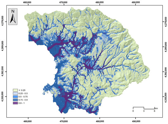
Figure 17.
Flood susceptibility map by the LR model.
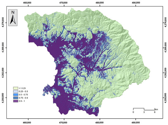
Figure 18.
Flood susceptibility map by the NB model.
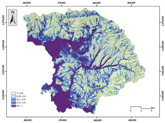
Figure 19.
Flood susceptibility map by the GB model.
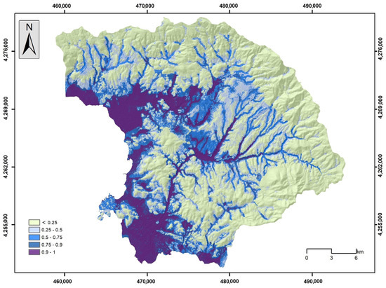
Figure 20.
Flood susceptibility map by the DLNN model.
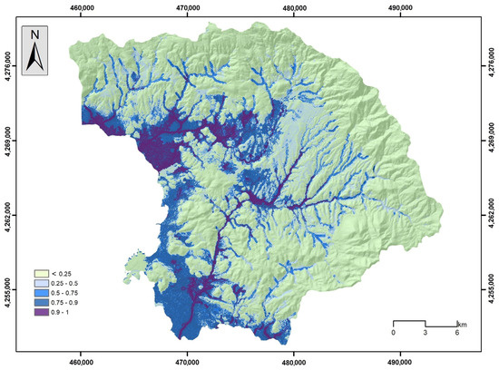
Figure 21.
Flood susceptibility map by the CNN model.

Table 4.
Flood susceptibility probability and relative density (multiplied by 100) of floods.
The results indicate that the high and very high susceptibility areas concentrate the highest frequency of floods, and very few floods appear within the very low susceptibility areas. This is proof that all models captured, in high precession, the link between the occurrence of historical flood events and the flood-related variables that shaped the susceptible zones for all the models built during the study. In all cases, the relative density of the high and very high susceptibility zones is over 75, which confirms the rationality of the flood susceptibility maps. The GB model achieved the highest relative density (55.72), with a probability over 0.91, followed by the 1D-CNN (58.08) and the NB model (46.80), whereas when considering a probability over 0.76 (high and very high susceptibility), the 1D-CNN model has the highest value (79.28), followed by the GB model (77.54) and the LR model (77.32).
According to the results, the learning and predictive performance of the models are quite different (Figure 22a,b, Table 5). All models had excellent performance regarding AUC values for the training dataset, ranging between 0.870 and 0.975, and for the test dataset, between 0.829 and 0.949. GB had the best learning accuracy in terms of AUC values (AUC values = 0.960), followed by the CNN (AUC value = 0.937) and the DLNN (AUC value = 0.930). The worst performance was achieved by the NB (AUC value = 0.899), followed by the LR (AUC value = 0.920). Concerning the test dataset, CNN had the best performance (AUC value = 0.924), followed by the LR (AUC value = 0.904) and the DLNN (AUC value = 0.899). Like the train dataset, the worst performance was achieved by NB (AUC value = 0.872), followed, however, by the GB model (AUC value = 0.877).
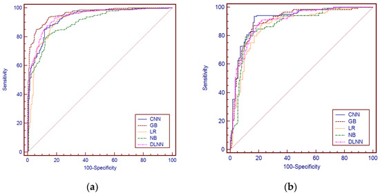
Figure 22.
(a) Sensitivity, 100-specificity, and ROC curves for the training dataset. (b) Sensitivity, 100-specificity, and ROC curves for the test dataset.

Table 5.
Training and test database AUC values.
From the pair-wise comparison of the predictions made by the CNN, GB, LR, NB and, DLNN models, statistically significant different results appear for the CNN, LR, NB, and DLNN models, whereas the CNN and GB models, according to the z statistic value, could not be considered statistically significantly different (Table 6).

Table 6.
Pair-wise comparison of ROC curves on the test database.
5. Discussion
According to the Directive 2007 of the European Commission, human activities, mainly those related to the development of human settlements and other assets within floodplains; the reduction in the natural capacity of the soil to retain water due to changes in land use; and the effects of climate change, contribute to the increase in the probability of flood events, with a corresponding increase in their negative effects. For the rational management of flood phenomena, it is first necessary to delineate the susceptible areas with as much precision as possible [83]. However, this is not an easy task, since the mechanism responsible for the occurrence and evolution of flood phenomena depends on rather complex natural processes that, in most cases, are not clearly understood [58]. Floods are characterized as multidimensional dynamic phenomena, a natural phenomenon which is difficult to prevent. RS data and GIS assist in exploring the extent of flooded areas and the post-event effects, whereas nonlinear machine learning algorithms have been proposed for flood modeling, with promising results [3]. In this context, our study focused on the application of ML models, specifically a 1D-CNN model whose effectiveness was compared with four state-of-the-art ML models, LR, NB, GB, and DLNN.
First, one must highlight that by leveraging the satellite images from the Copernicus Program and the Sentinels Scientific Data Hub, the study benefits from high spatial resolution, wide coverage, and frequent acquisitions, enabling the accurate identification and mapping of flooded areas. These advantages enhance the reliability and effectiveness of the flash flood susceptibility mapping approach that this study follows. The Copernicus Program follows an open data policy, making the satellite imagery and derived products freely accessible to the public. This accessibility encourages widespread use and collaboration among researchers, leading to advancements in flood assessment methodologies and enabling comparisons between different regions and studies.
Concerning the identification of flood areas, the study calculated the DNDWI index, which is based on B03 and B08 bands, to highlight water bodies and identify flooded areas. As described in [45], the NDWI index is ideal to delineate open water features and enhance their presence in remotely sensed digital imagery, using the reflected near-infrared radiation and visible green light to enhance the presence of such features while eliminating the presence of soil and terrestrial vegetation features.
The selection of specific satellite images was based on their availability, their being freely and openly accessed, and their spatial and temporal coverage. In addition, their fine spatial resolution, 10 m per pixel, provides more detailed information about the land surface, allowing for better discrimination of water bodies, infrastructure, and other land features. Also, their spectral bands, B03 and B08, were ideal to detect the presence of water and differentiate between water and other land features, due to their unique reflectance properties.
During the Pearson analysis, a high correlation between elevation and MFI (0.83) was detected. Douglas et al. [84] suggests that the presence of high correlation values may lead to an increased probability of flood occurrence. In our case, the observed high correlation had a minor influence on the outcome’s accuracy. Multi-collinearity analysis indicated that there was no significant correlation between any of the thirteen variables. The high Pearson value refers to the linear relation between the two variables, whether the multi-collinearity refers to a linear relationship between three or more variables. Thus, even if a high correlation is observed between elevation and MFI, the non-existing multi-collinearity implies that the problem is complex and could not be described by a linear model.
From the conducted importance analysis, elevation, distance to river network, land cover, lithology cover, and slope angle were the most important flood-related variables, according to the SHAP values. Similar findings have been found supporting the outcomes of the study, although an apparent difference among studies concerning the importance of flood-related variables could be the physical, morphological, and hydrological characteristics of the research areas. The elevation parameter is assigned the highest importance value by many authors; higher elevation receives a lower probability of occurrence of flooding, and vice versa [29,58]. Areas of lower elevation receive the amount of water that flows from the upper portions of a water basin. According to Lekkas et al. [41], the morphological settings played a significant role in the case of the August 2020 flood event in the research area. The water basins appear with steep slopes in their upstream section, which results in high flow velocities, increased erosion, and mass movement phenomena.
Distance to river network has also been recognized as a variable that could explain the presence of flood events with high accuracy. An increasing factor in shaping the degree of influence of the specific variable is the effect of anthropogenic activities. This is also recognized by Karkani et al. [85]. The authors report that human structures that are located along the river network reduced the critical cross-sections of the rivers, causing local overflows, which resulted in intense flood phenomena in the lowland areas.
Land cover appears to be a crucial variable that influences the occurrence of flooding. The absence of vegetation creates flooding areas, whereas urban areas covered by impervious materials increase the flow of surface runoff [86,87,88]. In our case, the predicted flooded areas are characterized by the presence of non-irrigated arable land (35%), complex cultivation patterns (27%), annual crops associated with permanent crops (13%), discontinuous urban fabric (8%), and olive groves (5%).
Another variable identified by the SHAP model was the lithology cover. In general, lithology cover has a high influence on flood phenomena, since it may influence runoff and infiltration rates and control sediment production within the water basin [57,89]. In total, 37% of the research area is covered by carbonate rock formations, mainly found in the upper portion of the research area, followed by Neogene formations (21%) and recent and old quaternary deposits (17%). The latter showed the highest frequency of observed floods (approximately 56% of the total observed flood areas), followed by the Neogene formations (26%). Karymbalis et al. [90], who investigated the geomorphic evolution of the Lilas river, report that climate, the highly erodible formations, and the steep slopes found in the upper sections of the water basin of Lilas are conditions that favor weathering and erosion processes. This produces huge volumes of sediments which are transported to the lower lands of the water basin.
Finally, slope was the fifth variable with significant influence in shaping the flood susceptibility index. As stated by several researchers, slopes influence the probability of flood occurrence. Areas characterized by a low slope angle have a higher probability of flood occurrence because of changes that appear in the infiltration rate and amount of runoff [91]. Moreover, the morphological settings of the areas are those found in a typical Mediterranean terrain, characterized by small water basins, less than 2000 km2 in size, which are associated with intense precipitation events and disastrous flash floods [85].
Concerning the generated flood susceptibility maps, they have a similar spatial distribution pattern; most flood-prone areas are identified in the lower land, close in distance to the river network. These two variables shape the extent of the flooded areas. The most susceptible areas are Politika, Psachna, Politika, Lefkanti, and Vasiliko.
Overall, the ML models showed a high predictive performance in terms of AUC values, since the values ranged between 0.872 and 0.924. The CNN model showed the highest performance, whereas statistically significant differences in the modelling process were detected for the all the models. The higher predictive performance of the CNN model could be attributed to the different learning patterns it uses and the specific structure of the data that was implemented. According to Wang et al. [12] the 1D data structure contains all the information concerning the flood-related variables, and the 1D-CNN topology evaluates the local relations between the flood-related variables. This is apparent in our case, where the 1D-CNN model successfully identified the flooded areas during the extreme rainfall event of August 2020.
DL models and, in our case, the 1D-CNN model is typically trained using large datasets and require significant computational resources, such as high-end GPUs and distributed computing systems. However, they have demonstrated remarkable success in a wide range of applications and are rapidly becoming a standard tool for data analysis and decision making in various fields, including healthcare, finance, transportation, and geoscience. Although LR and 1D-CNN are two different types of ML models, they appear to have a similar predictive performance. LR is a simple and interpretable model; however, it may not be able to capture complex relations between input features. The 1D-CNN model, on the other hand, can automatically learn feature representations that capture the complex spatial correlations between flood-related variables and the actual flooded areas and can achieve high accuracy in classification tasks. The CNN model and the benchmark models appeared with excellent predictive performance; however, there are several aspects that may improve their performance even further. One of the most important issues is the identification of the non-flash-flood areas, the presence of which is mandatory for classification problems using machine learning methods. In our case, the generation of non-flood areas was based on a random search method outside areas identified as Potential Significant Flood Risk according to criteria defined by the Directive 2007, which may have influenced the outcomes of all models. Comparing the computational time needed for modeling and prediction needed between the models, the CNN model requires more time than conventional machine learning methods. Thus, it is up to the researcher to decide the trade-off between time efficiency and performance. Regarding future work, it could focus on applying the 1D-CNN, based on the concept of Transfer Learning, to regions with different geo-environmental settings. New parameters derived from sophisticated remote sensing techniques and improving the quality of available data may assist in providing more accurate models, aspects that should be subjects of future work. The agenda of future works should also include the investigation of the influence of the number of classes created for each flash flood variable on the accuracy. Finally, future works should investigate the application of different classification methods that may combine statistical, probabilistic, and expert-based methods to improve the predictive accuracy of 1D-CNN models.
6. Conclusions
The main objective of the present study was to evaluate the performance of a 1D-CNN model and compare its performance with benchmark machine learning models (logistic regression, Naïve Bayes, gradient boosting, and deep learning neural network) in flood susceptibility assessments. According to the multi-collinearity analysis, no collinearity was detected among the flood-related variables, whereas elevation, distance to river network, land cover, lithology, and slope angle were estimated to be the most important variables, based on the results obtained using the SHAP method. The 1D-CNN model appeared to have the highest predictive performance in terms of AUC value (0.924), followed by the LR (0.904) and DLNN models (0.899). As mentioned in the discussion, the CNN’s performance is based on the model’s ability to appropriately shape the degree of influence of the flood-related variables not on the entire research area but according to the special characteristics and settings of the local areas within the wider research area. In summary, CNNs are a promising approach for flood susceptibility analysis, but their success depends on the availability and quality of the training data, as well as the computational resources available for training and inference. The information and knowledge gained from the outcomes of the present study could assist local authorities and government agencies in the direction of accurately identifying flash-flood-susceptible areas to implement in those areas appropriate flood management plans.
Author Contributions
Conceptualization, P.T. and A.-A.C.; methodology, P.T. and A.-A.C.; software, P.T. and A.-A.C.; investigation, data selection, P.T. and I.I.; writing—original draft preparation, P.T., I.I. and A.-A.C.; writing—review and editing, P.T., A.-A.C., I.I., I.M., W.C. and H.H. All authors have read and agreed to the published version of the manuscript.
Funding
This research received no external funding.
Data Availability Statement
Provided by the authors upon request.
Conflicts of Interest
The authors declare no conflict of interest.
References
- CRED. 2022 Disasters in Numbers; CRED: Brussels, Belgium, 2023; Available online: https://cred.be/sites/default/files/2022_EMDAT_report.pdf (accessed on 12 May 2023).
- Diakakis, M. Flood Hazard Assessment with the Use of Modeling Techniques; National and Kapodistrian University of Athens: Athens, Greece, 2012. [Google Scholar]
- Ilia, I.; Tsangaratos, P.; Tzampoglou, P.; Chen, W.; Hong, H. Flash Flood Susceptibility Mapping Using Stacking Ensemble Machine Learning Models. Geocarto Int. 2022, 37, 15010–15036. [Google Scholar] [CrossRef]
- Hoque, M.; Tasfia, S.; Ahmed, N.; Pradhan, B. Assessing Spatial Flood Vulnerability at KalaparaUpazila in Bangladesh Using an Analytic Hierarchy Process. Sensors 2019, 19, 1302. [Google Scholar] [CrossRef] [PubMed]
- Rahmati, O.; Darabi, H.; Panahi, M.; Kalantari, Z.; Naghibi, S.A.; Ferreira, C.S.S.; Kornejady, A.; Karimidastenaei, Z.; Mohammadi, F.; Stefanidis, S.; et al. Development of novel hybridized models for urban flood susceptibility mapping. Sci. Rep. 2020, 20, 12937. [Google Scholar] [CrossRef] [PubMed]
- Nandi, A.; Mandal, A.; Wilson, M.; Smith, D. Flood Hazard Mapping in Jamaica Using Principal Component Analysis and Logistic Regression. Environ. Earth Sci. 2016, 75, 465. [Google Scholar] [CrossRef]
- Lee, S.; Kim, J.-C.; Jung, H.-S.; Lee, M.J.; Lee, S. Spatial Prediction of Flood Susceptibility Using Random-Forest and Boosted-Tree Models in Seoul Metropolitan City, Korea. Geomat. Nat. Hazards Risk 2017, 8, 1185–1203. [Google Scholar] [CrossRef]
- Chen, W.; Hong, H.; Li, S.; Shahabi, H.; Wang, Y.; Wang, X.; Ahmad, B.B. Flood Susceptibility Modelling Using Novel Hybrid Approach of Reduced-Error Pruning Trees with Bagging and Random Subspace Ensembles. J. Hydrol. 2019, 575, 864–873. [Google Scholar] [CrossRef]
- Tehrany, M.S.; Jones, S.; Shabani, F. Identifying the Essential Flood Conditioning Factors for Flood Prone Area Mapping Using Machine Learning Techniques. Catena 2019, 175, 174–192. [Google Scholar] [CrossRef]
- Bui, D.T.; Ngo, P.-T.T.; Pham, T.D.; Jaafari, A.; Minh, N.Q.; Hoa, P.V.; Samui, P. A Novel Hybrid Approach Based on a Swarm Intelligence Optimized Extreme Learning Machine for Flash Flood Susceptibility Mapping. Catena 2019, 179, 184–196. [Google Scholar] [CrossRef]
- Shin, J.-Y.; Ro, Y.; Cha, J.-W.; Kim, K.-R.; Ha, J.-C. Assessing the Applicability of Random Forest, Stochastic Gradient Boosted Model, and Extreme Learning Machine Methods to the Quantitative Precipitation Estimation of the Radar Data: A Case Study to Gwangdeoksan Radar, South Korea, in 2018. Adv. Meteorol. 2019, 2019, 1–17. [Google Scholar] [CrossRef]
- Wang, Y.; Fang, Z.; Hong, H.; Peng, L. Flood Susceptibility Mapping Using Convolutional Neural Network Frameworks. J. Hydrol. 2020, 582, 124482. [Google Scholar] [CrossRef]
- Wang, Y.; Fang, Z.; Wang, M.; Peng, L.; Hong, H. Comparative Study of Landslide Susceptibility Mapping with Different Recurrent Neural Networks. Comput. Geosci. 2020, 138, 104445. [Google Scholar] [CrossRef]
- Costache, R.; Ngo, P.T.T.; Bui, D.T. Novel Ensembles of Deep Learning Neural Network and Statistical Learning for Flash-Flood Susceptibility Mapping. Water 2020, 12, 1549. [Google Scholar] [CrossRef]
- Khosravi, K.; Panahi, M.; Golkarian, A.; Keesstra, S.D.; Saco, P.M.; Bui, D.T.; Lee, S. Convolutional Neural Network Approach for Spatial Prediction of Flood Hazard at National Scale of Iran. J. Hydrol. 2020, 591, 125552. [Google Scholar] [CrossRef]
- Tabbussum, R.; Dar, A.Q. Performance Evaluation of Artificial Intelligence Paradigms—Artificial Neural Networks, Fuzzy Logic, and Adaptive Neuro-Fuzzy Inference System for Flood Prediction. Environ. Sci. Pollut. Res. 2021, 28, 25265–25282. [Google Scholar] [CrossRef]
- Li, H.; Zhu, L.; Dai, Z.; Gong, H.; Guo, T.; Guo, G.; Wang, J.; Teatini, P. Spatiotemporal Modeling of Land Subsidence Using a Geographically Weighted Deep Learning Method Based on PS-InSAR. Sci. Total Environ. 2021, 799, 149244. [Google Scholar] [CrossRef] [PubMed]
- Shao, Y.; Wang, Z.; Feng, Z.; Sun, L.; Yang, X.; Zheng, J.; Ma, T. Assessment of China’s Forest Fire Occurrence with Deep Learning, Geographic Information and Multisource Data. J. For. Res. 2023, 34, 963–976. [Google Scholar] [CrossRef]
- Senanayake, S.; Pradhan, B.; Alamri, A.; Park, H.-J. A New Application of Deep Neural Network (LSTM) and RUSLE Models in Soil Erosion Prediction. Sci. Total Environ. 2022, 845, 157220. [Google Scholar] [CrossRef] [PubMed]
- Bui, Q.-T.; Nguyen, Q.-H.; Nguyen, X.L.; Pham, V.D.; Nguyen, H.D.; Pham, V.-M. Verification of Novel Integrations of Swarm Intelligence Algorithms into Deep Learning Neural Network for Flood Susceptibility Mapping. J. Hydrol. 2020, 581, 124379. [Google Scholar] [CrossRef]
- Alzubaidi, L.; Zhang, J.; Humaidi, A.J.; Al-Dujaili, A.; Duan, Y.; Al-Shamma, O.; Santamaría, J.; Fadhel, M.A.; Al-Amidie, M.; Farhan, L. Review of Deep Learning: Concepts, CNN Architectures, Challenges, Applications, Future Directions. J. Big Data 2021, 8, 53. [Google Scholar] [CrossRef]
- Maggiori, E.; Tarabalka, Y.; Charpiat, G.; Alliez, P. Can Semantic Labeling Methods Generalize to Any City? The Inria Aerial Image Labeling Benchmark. In 2017 IEEE International Geoscience and Remote Sensing Symposium (IGARSS); IEEE: Fort Worth, TX, USA, 2017; pp. 3226–3229. [Google Scholar] [CrossRef]
- Long, J.; Shelhamer, E.; Darrell, T. Fully Convolutional Networks for Semantic Segmentation. In 2015 IEEE Conference on Computer Vision and Pattern Recognition (CVPR); IEEE: Boston, MA, USA, 2015; pp. 3431–3440. [Google Scholar]
- Ghorbanzadeh, O.; Blaschke, T.; Gholamnia, K.; Meena, S.; Tiede, D.; Aryal, J. Evaluation of Different Machine Learning Methods and Deep-Learning Convolutional Neural Networks for Landslide Detection. Remote Sens. 2019, 11, 196. [Google Scholar] [CrossRef]
- Guirado, E.; Tabik, S.; Alcaraz-Segura, D.; Cabello, J.; Herrera, F. Deep-Learning Convolutional Neural Networks for Scattered Shrub Detection with Google Earth Imagery. arXiv 2017, arXiv:1706.00917v1. [Google Scholar] [CrossRef]
- Wang, Y.; Fang, Z.; Hong, H. Comparison of Convolutional Neural Networks for Landslide Susceptibility Mapping in Yanshan County, China. Sci. Total Environ. 2019, 666, 975–993. [Google Scholar] [CrossRef]
- Zhang, G.; Wang, M.; Liu, K. Forest Fire Susceptibility Modeling Using a Convolutional Neural Network for Yunnan Province of China. Int. J. Disaster Risk Sci. 2019, 10, 386–403. [Google Scholar] [CrossRef]
- Fang, Z.; Wang, Y.; Peng, L.; Hong, H. Integration of Convolutional Neural Network and Conventional Machine Learning Classifiers for Landslide Susceptibility Mapping. Comput. Geosci. 2020, 139, 104470. [Google Scholar] [CrossRef]
- Chen, W.; Li, Y.; Xue, W.; Shahabi, H.; Li, S.; Hong, H.; Wang, X.; Bian, H.; Zhang, S.; Pradhan, B.; et al. Modeling Flood Susceptibility Using Data-Driven Approaches of Naïve Bayes Tree, Alternating Decision Tree, and Random Forest Methods. Sci. Total Environ. 2020, 701, 134979. [Google Scholar] [CrossRef]
- Youssef, A.M.; Pradhan, B.; Dikshit, A.; Al-Katheri, M.M.; Matar, S.S.; Mahdi, A.M. Landslide Susceptibility Mapping Using CNN-1D and 2D Deep Learning Algorithms: Comparison of Their Performance at Asir Region, KSA. Bull. Eng. Geol. Environ. 2022, 81, 165. [Google Scholar] [CrossRef]
- Youssef, A.M.; Pradhan, B.; Dikshit, A.; Mahdi, A.M. Comparative Study of Convolutional Neural Network (CNN) and Support Vector Machine (SVM) for Flood Susceptibility Mapping: A Case Study at Ras Gharib, Red Sea, Egypt. Geocarto Int. 2022, 37, 11088–11115. [Google Scholar] [CrossRef]
- Krizhevsky, A.; Sutskever, I.; Hinton, G.E. ImageNet Classification with Deep Convolutional Neural Networks. Commun. ACM 2017, 60, 84–90. [Google Scholar] [CrossRef]
- Adhikari, T. Designing a Convolutional Neural Network for Image Recognition: A Comparative Study of Different Architectures and Training Techniques. Soc. Sci. Res. 2023, 2023, 28. [Google Scholar] [CrossRef]
- Zhao, G.; Pang, B.; Xu, Z.; Peng, D.; Zuo, D. Urban Flood Susceptibility Assessment Based on Convolutional Neural Networks. J. Hydrol. 2020, 590, 125235. [Google Scholar] [CrossRef]
- Ullah, K.; Wang, Y.; Fang, Z.; Wang, L.; Rahman, M. Multi-Hazard Susceptibility Mapping Based on Convolutional Neural Networks. Geosci. Front. 2022, 13, 101425. [Google Scholar] [CrossRef]
- ESRI. ArcGIS Desktop: Release 10.5; Environmental Systems Research Institute: Redlands, CA, USA, 2015; Available online: https://desktop.arcgis.com/en/index.html (accessed on 29 June 2022).
- Hellenic Statistical Authority (ELSTAT). Available online: http://dlib.statistics.gr/Book/GRESYE_01_0005_00008%20.pdf (accessed on 2 May 2023).
- Institute of Geology and Subsurface Research, Island of Euboea, scale 1:200.000. 1967. Available online: https://catalogue.nla.gov.au/Record/8613577 (accessed on 12 November 2022).
- Ulbrich, U.; Lionello, P.; Belušić, D.; Jacobeit, J.; Knippertz, P.; Kuglitsch, F.G.; Leckebusch, G.C.; Luterbacher, J.; Maugeri, M.; Maheras, P.; et al. 5—Climate of the Mediterranean: Synoptic Patterns, Temperature, Precipitation, Winds, and Their Extremes. In The Climate of the Mediterranean Region; Lionello, P., Ed.; Elsevier: Oxford, UK, 2012; pp. 301–346. ISBN 9780124160422. [Google Scholar]
- Katsafados, P.; Kalogirou, S.; Papadopoulos, A.; Korres, G. Mapping Long-Term Atmospheric Variables over Greece. J. Maps 2012, 8, 181–184. [Google Scholar] [CrossRef]
- Lekkas, E.; Spyrou, N.-I.; Kotsi, E.; Filis, C.; Diakakis, M.; Lagouvardos, K.; Cartalis, C.; Kotroni, V.; Dafis, S.; Vassilakis, E.; et al. The August 9, 2020 Evia (Central Greece) Flood; Newsletter of Environmental; Disaster and Crises Management Strategies: Athens, Greece, 2020. [Google Scholar]
- Antoniadis, Z. Scale Development for Flash Flood Impacts; National and Kapodistrian University of Athens: Athens, Greece, 2016. [Google Scholar]
- Sideris, N.; Papageorgiou-Torpidi, N.; Skokou, T.; Papanikolaou, G.; Foteinopoulos, B. Special Secretariat for Water. Available online: https://floods.ypeka.gr/index.php?option=com_content&view=article&id=15&Itemid=507 (accessed on 30 December 2020).
- European Union Directive. 2007/60/EC of the European Counil and European Parliment of 23 October 2007 on the assessment and management of flood risks. Off. J. Eur. Union 2007, 288, 27–34. [Google Scholar]
- McFeeters, S.K. The Use of the Normalized Difference Water Index (NDWI) in the Delineation of Open Water Features. Int. J. Remote Sens. 1996, 17, 1425–1432. [Google Scholar] [CrossRef]
- Twumasi, Y.A.; Merem, E.C.; Namwamba, J.B.; Asare-Ansah, A.B.; Annan, J.B.; Ning, Z.H.; Armah, R.N.D.; Apraku, C.Y.; Yeboah, H.B.; Atayi, J.; et al. Flood Mapping in Mozambique Using Copernicus Sentinel-2 Satellite Data. ARS 2022, 11, 80–105. [Google Scholar] [CrossRef]
- Copernicus Land Monitoring Service—part of the Copernicus Programme. Available online: https://land.copernicus.eu/pan-european/corine-land-cover/clc2018 (accessed on 20 December 2022).
- Bonham-Carter, G.F. Geographic Information Systems for Geoscientists: Modelling with GIS, Vol. 13, Computer Methods in the Geosciences; Pergamon Press: Oxford, UK, 1994; p. 398. [Google Scholar]
- Ilia, I.; Tsangaratos, P. Applying Weight of Evidence Method and Sensitivity Analysis to Produce a Landslide Susceptibility Map. Landslides 2016, 13, 379–397. [Google Scholar] [CrossRef]
- Ilia, I.; Tsangaratos, P.; Koumantakis, I.; Rozos, D. Application of A Bayesian Approach in Gis Based Model For Evaluating Landslide Susceptibility. Case Study Kimi Area, Euboea, Greece. Geosociety 2017, 43, 1590. [Google Scholar] [CrossRef]
- Agterberg, F.P.; Bonham-Carter, G.F.; Wright, D.F. Statistical Pattern Integration for Mineral Exploration. In Computer Applications in Resource Estimation; Gaál, G., Merriam, D.F., Eds.; Pergamon: Amsterdam, The Netherlands, 1990; pp. 1–21. ISBN 978-0-08-037245-7. [Google Scholar]
- ALOS-PALSAR—Earth Data. Available online: https://asf.alaska.edu/data-sets/sar-data-sets/alos-palsar/ (accessed on 20 December 2022).
- Fick, S.E.; Hijmans, R.J. WorldClim 2: New 1-km Spatial Resolution Climate Surfaces for Global Land Areas. Int. J. Climatol. 2017, 37, 4302–4315. [Google Scholar] [CrossRef]
- Ballabio, C.; Panagos, P.; Monatanarella, L. Mapping Topsoil Physical Properties at European Scale Using the LUCAS Database. Geoderma 2016, 261, 110–123. [Google Scholar] [CrossRef]
- Choubin, B.; Moradi, E.; Golshan, M.; Adamowski, J.; Sajedi-Hosseini, F.; Mosavi, A. An Ensemble Prediction of Flood Susceptibility Using Multivariate Discriminant Analysis, Classification and Regression Trees, and Support Vector Machines. Sci. Total Environ. 2019, 651, 2087–2096. [Google Scholar] [CrossRef]
- Chapi, K.; Singh, V.P.; Shirzadi, A.; Shahabi, H.; Bui, D.T.; Pham, B.T.; Khosravi, K. A Novel Hybrid Artificial Intelligence Approach for Flood Susceptibility Assessment. Environ. Model. Softw. 2017, 95, 229–245. [Google Scholar] [CrossRef]
- Khosravi, K.; Pham, B.T.; Chapi, K.; Shirzadi, A.; Shahabi, H.; Revhaug, I.; Prakash, I.; Tien Bui, D. A Comparative Assessment of Decision Trees Algorithms for Flash Flood Susceptibility Modeling at Haraz Watershed, Northern Iran. Sci. Total Environ. 2018, 627, 744–755. [Google Scholar] [CrossRef] [PubMed]
- Bui, D.T.; Tsangaratos, P.; Ngo, P.-T.T.; Pham, T.D.; Pham, B.T. Flash Flood Susceptibility Modeling Using an Optimized Fuzzy Rule Based Feature Selection Technique and Tree Based Ensemble Methods. Sci. Total Environ. 2019, 668, 1038–1054. [Google Scholar] [CrossRef]
- Tehrany, M.S.; Pradhan, B.; Mansor, S.; Ahmad, N. Flood Susceptibility Assessment Using GIS-Based Support Vector Machine Model with Different Kernel Types. Catena 2015, 125, 91–101. [Google Scholar] [CrossRef]
- Beven, K.J.; Kirkby, M.J. A Physically Based, Variable Contributing Area Model of Basin Hydrology/Un Modèle à Base Physique de Zone d’appel Variable de l’hydrologie Du Bassin Versant. Hydrol. Sci. Bull. 1979, 24, 43–69. [Google Scholar] [CrossRef]
- Moore, I.D.; Grayson, R.B.; Ladson, A.R. Digital Terrain Modelling: A Review of Hydrological, Geomorphological, and Biological Applications. Hydrol. Process. 1991, 5, 3–30. [Google Scholar] [CrossRef]
- Weiss, A. Topographic Position and Landforms Analysis. Available online: http://jennessent.com/downloads/TPI-poster-TNC_18x22.pdf (accessed on 9 October 2022).
- Zwolinski, Z.; Stefańska, E. Relevance of Moving Window Size in Landform Classification by TPI. In Geomorphometry for Geosciences; Jasiewicz, J., Zwoliński, Z., Mitasova, H., Hengl, T., Eds.; Bogucki Wydawnictwo Naukowe: Poznań, Poland, 2015; pp. 273–277. [Google Scholar]
- Newman, D.R.; Lindsay, J.B.; Cockburn, J.M.H. Evaluating Metrics of Local Topographic Position for Multiscale Geomorphometric Analysis. Geomorphology 2018, 312, 40–50. [Google Scholar] [CrossRef]
- Alam, A.; Ahmed, B.; Sammonds, P. Flash Flood Susceptibility Assessment Using the Parameters of Drainage Basin Morphometry in SE Bangladesh. Quat. Int. 2021, 575, 295–307. [Google Scholar] [CrossRef]
- Rahmati, O.; Pourghasemi, H.R.; Zeinivand, H. Flood Susceptibility Mapping Using Frequency Ratio and Weights-of-Evidence Models in the Golastan Province, Iran. Geocarto Int. 2016, 31, 42–70. [Google Scholar] [CrossRef]
- Ouma, Y.; Tateishi, R. Urban Flood Vulnerability and Risk Mapping Using Integrated Multi-Parametric AHP and GIS: Methodological Overview and Case Study Assessment. Water 2014, 6, 1515–1545. [Google Scholar] [CrossRef]
- Tariq, A.; Yan, J.; Ghaffar, B.; Qin, S.; Mousa, B.G.; Sharifi, A.; Huq, M.E.; Aslam, M. Flash Flood Susceptibility Assessment and Zonation by Integrating Analytic Hierarchy Process and Frequency Ratio Model with Diverse Spatial Data. Water 2022, 14, 3069. [Google Scholar] [CrossRef]
- Fernandez, H.; Martins, F.; Isodoro, J. Using the Modified Fournier Index to model rainfall aggressiveness with scarce rainfall data. In Proceedings of the 20th EGU General Assembly (EGU 2018), Vienna, Austria, 8–13 April 2018. [Google Scholar]
- Dimitriou, E. Precipitation Trends and Flood Hazard Assessment in a Greek World Heritage Site. Climate 2022, 10, 194. [Google Scholar] [CrossRef]
- Aydin, H.E.; Iban, M.C. Predicting and Analyzing Flood Susceptibility Using Boosting-Based Ensemble Machine Learning Algorithms with SHapley Additive ExPlanations. Nat. Hazards 2023, 116, 2957–2991. [Google Scholar] [CrossRef]
- Shapley, L.S. Stochastic Games. Proc. Natl. Acad. Sci. USA 1953, 39, 1095–1100. [Google Scholar] [CrossRef]
- Chen, T.; He, T.; Benesty, M.; Khotilovich, V.; Tang, Y.; Cho, H.; Chen, K.; Mitchell, R.; Cano, I.; Zhou, T. Xgboost: Extreme Gradient Boosting. R package version 1.7.3.1. Available online: https://CRAN.R-project.org/package=xgboost (accessed on 12 May 2023).
- Hubel, D.H.; Wiesel, T.N. Receptive Fields of Single Neurones in the Cat’s Striate Cortex. Physiol. J. 1959, 148, 574–591. [Google Scholar] [CrossRef] [PubMed]
- Chau, K.T.; Chan, J.E. Regional Bias of Landslide Data in Generating Susceptibility Maps Using Logistic Regression: Case of Hong Kong Island. Landslides 2005, 2, 280–290. [Google Scholar] [CrossRef]
- Cheeseman, P.C.; Stutz, J.C. Bayesian Classification (AutoClass): Theory and Results. In Advances in Knowledge Discovery and Data Mining; Springer: Berlin/Heidelberg, Germany, 1996. [Google Scholar]
- Tsangaratos, P.; Ilia, I. Comparison of a Logistic Regression and Naïve Bayes Classifier in Landslide Susceptibility Assessments: The Influence of Models Complexity and Training Dataset Size. Catena 2016, 145, 164–179. [Google Scholar] [CrossRef]
- Friedman, J.H. Greedy Function Approximation: A Gradient Boosting Machine. Ann. Statist. 2001, 29, 1189–1232. [Google Scholar] [CrossRef]
- Singaravel, S.; Suykens, J.; Geyer, P. Deep-Learning Neural-Network Architectures and Methods: Using Component-Based Models in Building-Design Energy Prediction. Adv. Eng. Inform. 2018, 38, 81–90. [Google Scholar] [CrossRef]
- Heaton, J. Ian Goodfellow, Yoshua Bengio, and Aaron Courville: Deep Learning: The MIT Press: Cambridge, MA, USA, 2016; p. 800. ISBN: 0262035618. Genet. Program. Evolvable Mach. 2018, 19, 305–307. [Google Scholar] [CrossRef]
- Hahnloser, R.H.R.; Sarpeshkar, R.; Mahowald, M.A.; Douglas, R.J.; Seung, H.S. Digital Selection and Analogue Amplification Coexist in a Cortex-Inspired Silicon Circuit. Nature 2000, 405, 947–951. [Google Scholar] [CrossRef]
- Hinton, G.; Deng, L.; Yu, D.; Dahl, G.E.; Mohamed, A.; Jaitly, N.; Senior, A.; Vanhoucke, V.; Nguyen, P.; Sainath, T.N.; et al. Deep Neural Networks for Acoustic Modeling in Speech Recognition: The Shared Views of Four Research Groups. IEEE Signal Process. Mag. 2012, 29, 82–97. [Google Scholar] [CrossRef]
- Mirzaei, S.; Vafakhah, M.; Pradhan, B.; Alavi, S.J. Flood Susceptibility Assessment Using Extreme Gradient Boosting (EGB), Iran. Earth Sci. Inform. 2021, 14, 51–67. [Google Scholar] [CrossRef]
- Douglas, E.M.; Vogel, R.M.; Kroll, C.N. Trends in Floods and Low Flows in the United States: Impact of Spatial Correlation. J. Hydrol. 2000, 240, 90–105. [Google Scholar] [CrossRef]
- Karkani, A.; Evelpidou, N.; Tzouxanioti, M.; Petropoulos, A.; Santangelo, N.; Maroukian, H.; Spyrou, E.; Lakidi, L. Flash Flood Susceptibility Evaluation in Human-Affected Areas Using Geomorphological Methods—The Case of 9 August 2020, Euboea, Greece. A GIS-Based Approach. GeoHazards 2021, 2, 366–382. [Google Scholar] [CrossRef]
- Mojaddadi, H.; Pradhan, B.; Nampak, H.; Ahmad, N.; Ghazali, A.H. bin. Ensemble Machine-Learning-Based Geospatial Approach for Flood Risk Assessment Using Multi-Sensor Remote-Sensing Data and GIS. Geomat. Nat. Hazards Risk 2017, 8, 1080–1102. [Google Scholar] [CrossRef]
- Mrozik, K.D. Problems of Local Flooding in Functional Urban Areas in Poland. Water 2022, 14, 2453. [Google Scholar] [CrossRef]
- Petrović, A.M. Challenges of torrential flood risk management in Serbia. Journal of the Geographical Institute “Jovan Cvijic”. SASA 2015, 65, 131–143. [Google Scholar] [CrossRef]
- Miller, J.R.; Ritter, D.F.; Kochel, R.C. Morphometric Assessment of Lithologic Controls on Drainage Basin Evolution in the Crawford Upland, South-Central Indiana. Am. J. Sci. 1990, 290, 569–599. [Google Scholar] [CrossRef]
- Karymbalis, E.; Valkanou, K.; Tsodoulos, I.; Iliopoulos, G.; Tsanakas, K.; Batzakis, V.; Tsironis, G.; Gallousi, C.; Stamoulis, K.; Ioannides, K. Geomorphic Evolution of the Lilas River Fan Delta (Central Evia Island, Greece). Geosciences 2018, 8, 361. [Google Scholar] [CrossRef]
- Hong, H.; Tsangaratos, P.; Ilia, I.; Liu, J.; Zhu, A.-X.; Chen, W. Application of Fuzzy Weight of Evidence and Data Mining Techniques in Construction of Flood Susceptibility Map of Poyang County, China. Sci. Total Environ. 2018, 625, 575–588. [Google Scholar] [CrossRef] [PubMed]
Disclaimer/Publisher’s Note: The statements, opinions and data contained in all publications are solely those of the individual author(s) and contributor(s) and not of MDPI and/or the editor(s). MDPI and/or the editor(s) disclaim responsibility for any injury to people or property resulting from any ideas, methods, instructions or products referred to in the content. |
© 2023 by the authors. Licensee MDPI, Basel, Switzerland. This article is an open access article distributed under the terms and conditions of the Creative Commons Attribution (CC BY) license (https://creativecommons.org/licenses/by/4.0/).