Abstract
In recent years, the applications of lidars for remote sensing of the environment have been expanding and deepening. Among them, continuous-wave (CW) range-resolved (RR) S-lidars (S comes from Scheimpflug) have proven to be a new and promising class of non-contact and non-perturbing laser sensors. They use low-power CW diode lasers, an unconventional depth-of-field extension technique and the latest advances in nanophotonic technologies to realize compact and cost-effective remote sensors. The purpose of this paper is to propose a generalized methodology to justify the selection of a set of non-energetic S-lidar parameters for a wide range of applications and distance scales, from a bench-top test bed to a 10-km path. To set the desired far and near borders of operating range by adjusting the optical transceiver, it was shown how to properly select the lens plane and image plane tilt angles, as well as the focal length, the lidar base, etc. For a generalized analysis of characteristic relations between S-lidar parameters, we introduced several dimensionless factors and criteria applicable to different range scales, including an S-lidar-specific magnification factor, angular function, dynamic range, “one and a half” condition, range-domain quality factor, etc. It made possible to show how to reasonably select named and dependent non-energetic parameters, adapting them to specific applications. Finally, we turned to the synthesis task by demonstrating ways to achieve a compromise between a wide dynamic range and high range resolution requirements. The results of the conducted analysis and synthesis allow increasing the validity of design solutions for further promotion of S-lidars for environmental remote sensing and their better adaptation to a broad spectrum of specific applications and range scales.
1. Introduction: Specific Features of S-Lidar-Based Remote Sensing
The S-lidars under discussion (S comes from Scheimpflug) have established themselves as a promising class of laser remote sensing tools for range-resolved (RR) environmental monitoring. Along with varieties of classic pulsed lidars [1,2,3,4,5,6], the research and development of S-lidars carried out in recent years have allowed this class of remote sensors to form their own niche. Many articles have now been published confirming a wide range of S-lidar applications, including terrestrial laser scanning and displacement monitoring [7,8,9,10], vegetation mapping, plants profiling and land cover change analysis [11,12,13,14], atmospheric remote sensing [15,16,17,18], CO2 sensing [19], urban environment monitoring [19,20,21], ocean, aquatic flora and fauna studies [13,14,22,23], oil pollution discrimination [24], UAV lidar applications [14,25], combustion diagnostics [26], insects monitoring [27], archiving [28], capabilities for remote air pollution detection [29], limitations under sky background [30], etc.
Outwardly, S-lidars are characterized by the use of low-power continuous-wave (CW) lasers, obvious compactness and comparative cheapness. An inside look notes the use of a technique for expanding the depth of field (DoF) of sharply focused images, unconventional for preceding lidars and borrowed from professional photography. This technique is based on the so-called Scheimpflug and Hinge principles [31,32]. Together with triangular distance control approaches and position-sensitive photodetection, this allows S-lidars to obtain detailed range profiles of received echo signals.
Figure 1 illustrates the general principles of S-lidar operation.

Figure 1.
Generalized representation of S-lidar operation principle.
Here, α is the image plane tilt angle; β is the lens plane tilt angle; Rmin is the near border of the operation range; R0 is the receiver alignment distance; Rmax is the far border of the operation range; ∆R is the range resolution; L is the lidar base; Ldet is the distance to array center; f is the focal length; pΣ is the total size of array detector; p1 is the single pixel size; n is the number of cells.
It may be noted that in many of the mentioned publications [7,8,9,10,11,12,13,14,15,16,17,18,19,20,21,22,23,24,25,26,27,28] on S-lidars, after a brief explanation of operation peculiarities, it is said that a laser diagnostic system with such-and-such hardware parameters was built to solve such-and-such a specific problem, and then, what has come out of it is presented. At the same time, questions are not always raised and discussed how effective the obtained engineering solutions are, and to what extent the achieved performance of designed systems and presented diagnostic results can limit the suitability of such S-lidars for chosen task-oriented applications or, on the contrary, open new prospects.
Since S-lidars implement the triangular principle of range control, we note that it is still an open question how to analytically predict interdependent tilting angles of the lens plane and the image plane to provide the required depth of field and how the optical and design parameters of a lidar system should be chosen, adapting to various range scales for different applications, although it seems quite understandable when the initial stage of developing a new system for a particular application is based on certain available hardware components and existing instrumentation.
In some previously mentioned papers, it was noted that, unlike the traditional classes of laser remote sensors, the current range resolution ΔR in S-lidars is proportional to the range square. At the same time, the issue of what is practically achievable range resolution ΔR at the far border of DoF is quite often not mentioned for some reason. Therefore, sometimes a scale of array cell numbers instead of a distance scale is used in graphs to illustrate range-dependent distribution.
The issues of ensuring acceptable ΔR(Rmax) for specific Rmax scales regardless of application are also generally not discussed. Then, if the ΔR value at the far border ΔR(Rmax) is unacceptably large, the lidar signals received from afar can be considered uninformative in terms of the low quality of spatially-resolved data. This can lead to a noticeable reduction in significance of the achieved results considered from the energy point of view, when the accuracy of echo-signal detection and primary processing can remain quite high.
Low-power, small-sized, light-weight and cost-effective S-lidars can be used in a wide variety of human activities. Thus, the range-domain scale of particular applications can also vary widely. For a wide variety of laser remote sensing applications, we intend to form a generalized methodology for the reasonable selection of a set of non-energy parameters for environmental S-lidars, affecting their range–domain performance from bench-top prototypes to 10 km traces.
2. Methods and Approaches
2.1. Problem Definition: Development of Methodology for Design of CW RR S-Lidars for Various Range Scales: From a 1 m Tabletop Test Bench to a 10 km Path
S-lidars realize the triangular principle of distance control, using relatively low-power continuous-wave diode lasers and array detectors [33,34,35]. To implement range imaging, the depth of field of sharply focused images is significantly expanded by tilting the lens and image planes [17,36,37]. Each i-th pixel of an array forms its own field of view, tracks changes in partial volume along the sensing path and predetermines the current range resolution ∆Ri [17,38]. Earlier in our papers [38,39], we have studies basic features of range-domain characteristics of S-lidars.
We consider the problem of selecting non-energetic hardware parameters of S-lidars to provide a range–domain tactical performance for any applications: from a tabletop test bed to a 10 km path. Suppose that the necessary tactical requirements are set for any application as follows (Figure 1): Rmax is the far border of the depth of field (DoF); the dynamic range D required
with Rmin as a near border of DoF. We will also consider the required spatial resolution ∆R(Rmax) at the far border Rmax of the depth of field as given, taking into account the S-type-specific features of the range-domain formation. To somewhat reduce the uncertainty with hardware parameters, we will consider as given the active length pΣ of a linear array detector used.
D = Rmax/Rmin
To adapt S-lidar tools to a wide variety of applications with different depth of field,
with a possible far border Rmax = 1 m/10 m/100 m/1 km/10 km requires justifying the choice of a whole set of non-energetic parameters. These parameters affecting the range-domain characteristics are presented in Table 1.

Table 1.
Non-energetic parameters affecting range–domain performance of S-lidar.
The S-lidar parameters to be determined:
- -
- Tilt angle α of the image plane to the lens plane;
- -
- Tilt angle β of the lens plane to the plane of the sensing object (Figure 1);
- -
- Focal length f of the receiving optics;
- -
- Lidar base L as a distance from the lens center to the laser beam, measured in the lens plane;
- -
- Distance Ldet to the center of array detector;
- -
- Single pixel size p1,
- -
- Total number of pixels n of a linear array detector.
It is also necessary to know what is the alignment distance R0 of receiving optics as the point of intersection of its optical axis with laser beam.
2.2. S-Lidar Alignment for the Desired Range: Eliminating Uncertainty When Choosing Tilt Angles of Receiving Optics and Detecting Array
2.2.1. Effect of Introduced S-Lidar-Specific Notions: Magnification M and Angular Function S(x)
To characterize the range imaging capabilities characteristic of S-lidars, let us introduce an index M as the ratio of the realized depth-of-field DR to the total length pΣ of linear array detector. With (1) and (2) in mind, let us write the following:
Obviously, the effect of the dimensionless dynamic range D on M is quite noticeable up to its moderate values D < 10, and at larger values of D, one can assume M = Rmax/pΣ.
Consider how the introduced factor M affects the character of interdependence of tilt angles α and β, using, in particular, the S-lidar geometry in Figure 2.
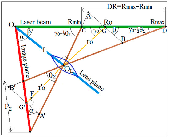
Figure 2.
Geometric relations in S-lidar.
As you can see, all geometric constructions are based on the laser beam, the lens and image planes, which are highlighted in green, blue and red. The receiving optical axis is drawn through the lens center (point OL) and the center G’ of the array detector. This line is perpendicular to the lens plane and intersects the laser beam at point G at a distance Ro.
Note that we deliberately changed the geometric proportions in Figure 2 so that they are greatly reduced on the range scale and become elongated in relation to the transceiver. Thus, we sought to illustrate the technique used in S-lidars to cover the greater depth of field (DoF) of sharply focused images. In fact, in S-lidars, probably except for desktop prototypes, both near Rmin and far Rmax borders of DoF can be set very far, many hundreds of meters and kilometers from the sensor. Because of this, the real receiving field-of-view (FoV) angle θΣ (seemingly large in Figure 2) turns out to be very small, so that the wide depth of field is provided by proper tilts of the receiving optics and the array detector, which are much larger than θΣ. In contrast to remote DoF borders, the basic distance L between the laser and the receiving optics in S-lidars usually does not exceed 1 m, and sometimes a little more. To describe the interdependence of angles α and β, let us analyze the geometric relationships within triangles CDOL and C’D’OL, intersected by the receiving optical axis GG’. Taking into account the comments made above, we can write the following as the very first approximation to be considered acceptable for lens tilt angles β that are not too close to the right angle
It should also be noted that here the alignment angle γ0 = π/2 − β of the receiver’s optical axis is assumed by default to always be greater than θΣ/2 as half of the receiving angle of view.
Then, (3) can be rewritten as follows:
For further convenience in using (5), we introduce another parameter, also characterizing the specificity of S-lidars, and call it the angular S-function:
where x is the arbitrary tilt angle. The behavior of S(x) is shown in Figure 3.
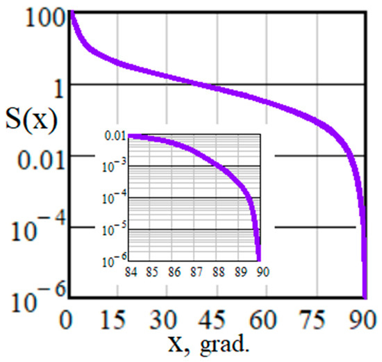
Figure 3.
S-function behavior over a wide range of angles and when approaching 90°.
Then it is clear that, according to (3) and (6), the index M given earlier predetermines the relationship between functions S(α) and S(β) of the detector plane α and the lens plane β angles:
The M-index value, being adapted to various range–domain applications, determines the realized operation range width DR of S-lidars when using the available array of length pΣ. Therefore, if we solve Equation (7) with respect to sinβ, then with the chosen array tilt angle α it appears that the lens tilt angle β should satisfy such a relation:
This will ensure that the length of sharply focused DoF is equal to DR = M·pΣ. Similarly to (8), if the tilt angle β is chosen first, then the angle α obeys this equation:
2.2.2. Sensitivity of Interdependent Tilt Angles α and β to Range–Domain Scales
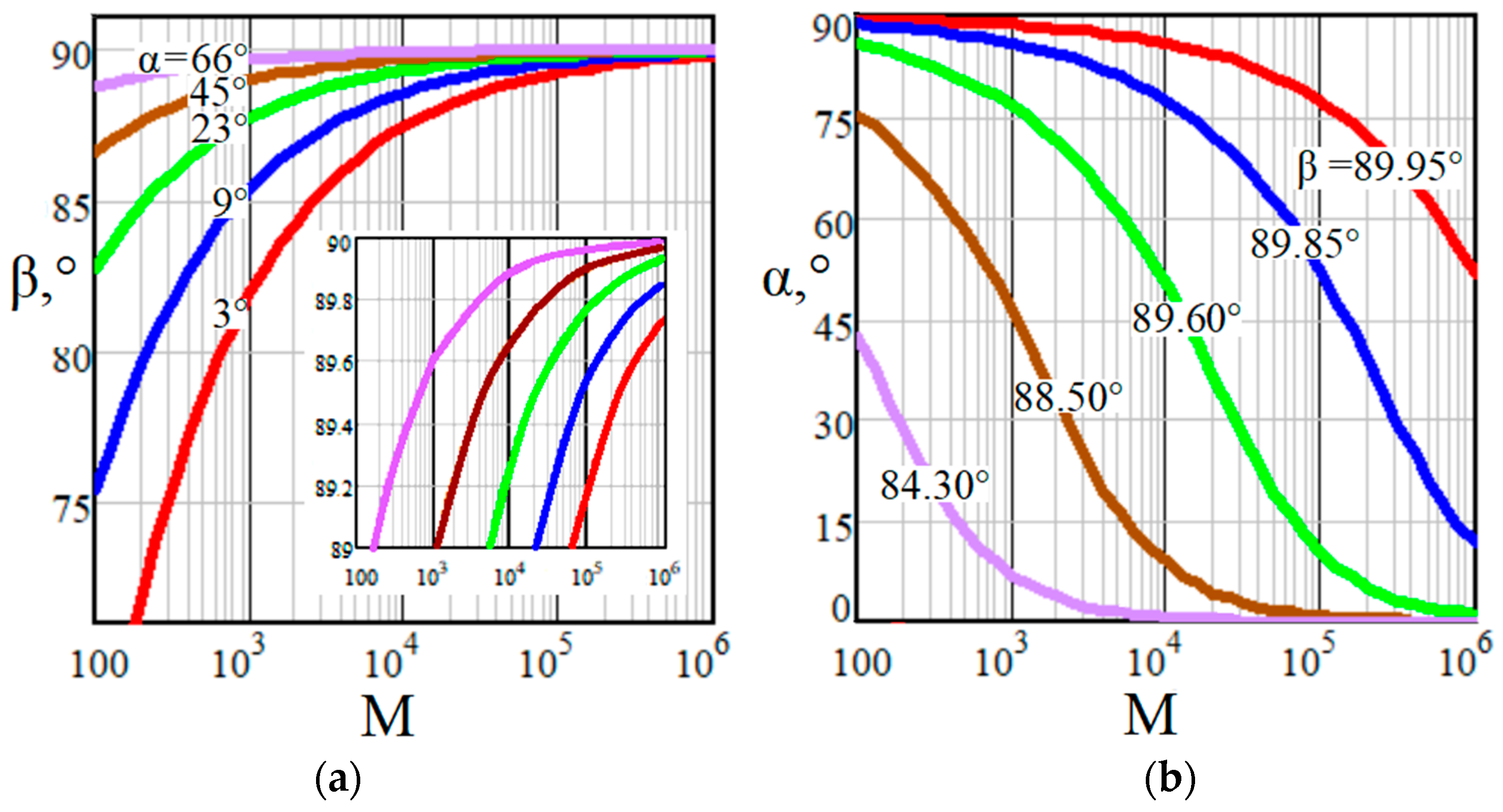
Let us show to what extent the application-specific DoF scale affects the choice of tilt angles α and β. Justifications (8) and (9) for selecting α and β to ensure the necessary operation range width are graphically shown in Figure 4. In both cases, we see that index M determines trends in the tilt angles’ variability.
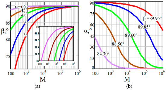
Figure 4.
(a,b) Tilt angles of the lens and image planes as functions of M-index.
Both Figure 4a,b certify that according to (3) and Figure 2, at Rmax > 1 km, the M-parameter values become very large, so that M → 105, and even M → 106. Then, with a rather wide variability of angles α from small to large, the required tilt angles β become increasingly close to 90°, and the receiving optical axis approaches the probing beam direction (γ0 → 0°). If, however, S-lidars are developed for applications with significantly closer Rmax < 100 m and in relatively narrow spatial regions (e.g., with 1.5 < D < 3), the M-parameter takes much smaller values: M → 102…103. This can be realized at more distant from 90° values of tilt angles β.
2.2.3. A New “One and a Half” Criterion to Choose Proper Tilting Angles α and β
To continue the reasoning and illustrations for the previous section, let us consider the problem of interrelated selection of tilt angles α and β from another side. If the lidar developer first chose the tilt angle α, then the associated tilt angle β can be represented in this form:
which follows from (3) and (8).
We noted above that in each specific application, the range of lens tilt angles β turns out to be quite narrow. Indeed, the procedures for selecting and adjusting the angle β according to Scheimpflug principles [31,32] cause dissimilar changes in the focal length f and the base L, orthogonal to each other geometrically. As a criterion highlighting the range of acceptable angles β, we propose the “one and a half” condition applied to the tangent α characterizing the tilt angle of the image plane:
which provides no more than one-and-a-half ratio of the transceiver’s overall dimensions in the longitudinal and transverse directions as a characteristic of its peculiar compactness.
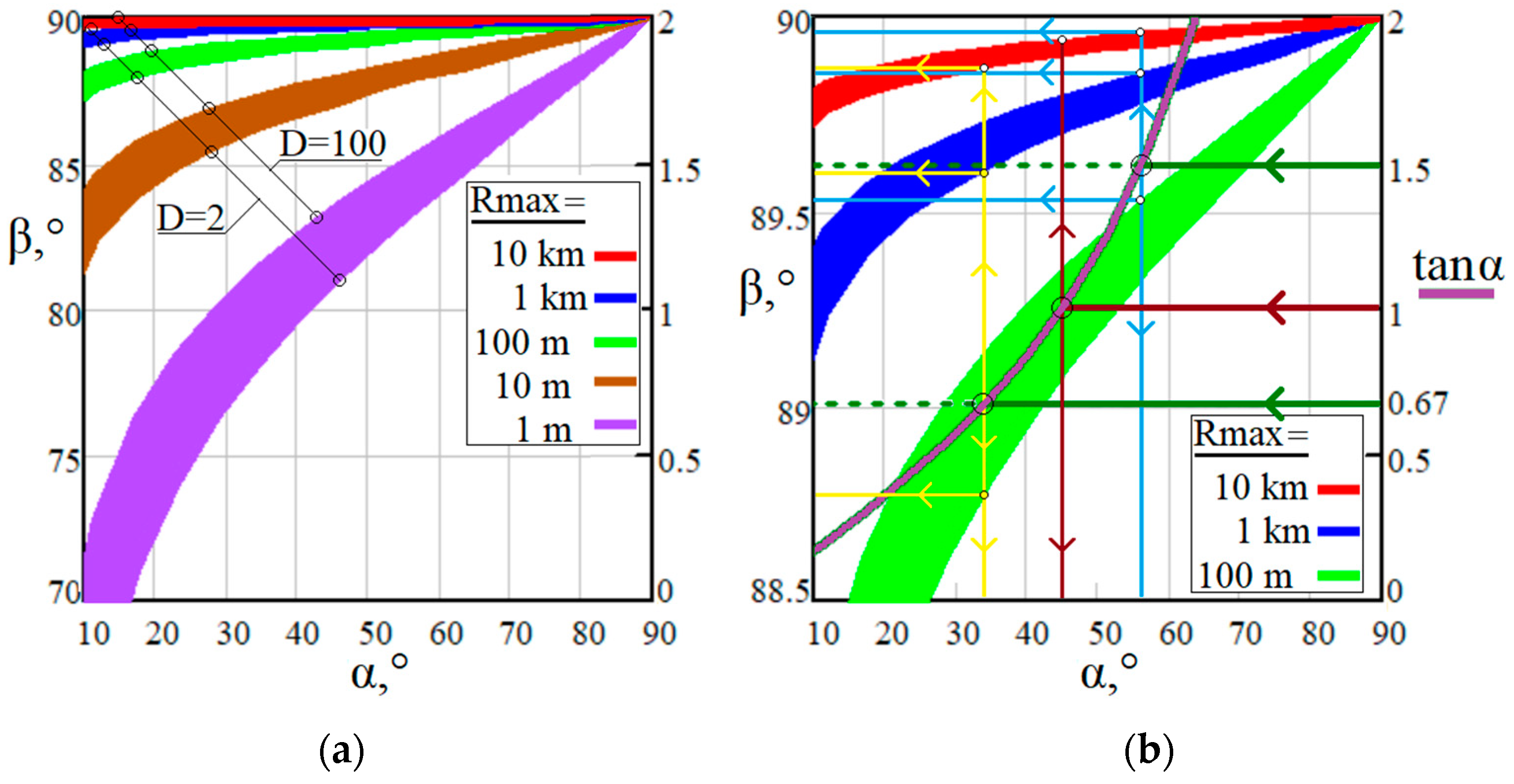
Figure 5 shows the dependencies β = f(α) applicable to diagnostics over a wide range from a tabletop test bench to a 10 km path. Curves are presented at a tenfold range sampling (Rmax = 10x, x = 0…4) at variations D = 2…100.

Figure 5.
Dependences β = f(α) within a wide variability range of tilt angles β, suitable for relatively close Rmax (a); detailed consideration of β = f(α) within a narrow range of tilt angles β, applicable to more distant Rmax (b); pΣ = 1.8 cm.
The “one and a half” condition is illustrated in Figure 5b in the graph tanα = f(α). The horizontals tanα = 1.5 and tanα = 0.67 allow for an acceptable range of image angles α with αmin = 33.8° and αmax = 56.3°. On this basis, the intersections of vertical lines α = αmin and α = αmax with β(α) bands for very different Rmax indicate acceptable tilt angles β of the receiving optics. The lower and upper bounds of each band correspond to D = 2 and D = 100. The simplest situation with α = π/4 at tanα = 1 is also shown for comparison.
Table 2 shows the admissible limits of β for the most different S-lidar operation ranges. In addition, tilt angles β at tan(α = π/4) = 1 are added.

Table 2.
Borders of tilt angle β to provide the required tactical parameters of S-lidars.
Thus, the tilt β at large DR is very close to π/2, which is equivalent to setting the angle γ0 of the receiving optical axis very close to zero. They must be set very precisely, which according to (10), ensures the far Rmax and near Rmin borders of the depth of field predetermined in M-parameter according to (1)–(3). On the other hand, Equation (10) also underlines the high sensitivity of practically realizable values of Rmax and D to the adjustment accuracy of these angles.
Note that when angle α = π/4 is preferred, which is common in optics, it turns out that S(π/4) = √2/2 according to (6). Then, it follows from (8) that the angle β is determined by the dimensionless parameter M = DR/pΣ ≫ 1 in a very simple way:
2.3. How to Select Suitable Hardware Parameters for S-Lidars with Different Range–Domain Scales from 1 m Up to 10 km
Thus, we see how the angles α and β are related, and that there are interdependent pairs of values (α; β) for the required Rmax and D that allow us to provide the required depth of field through parameter M. Let us consider how, in this case, to choose the optical and structural parameters of the lidar device given in Table 1.
2.3.1. Adaptive Choice of Both Focal Length and Lidar Base to Specific Range–Domain Requirements
It became clear that by selecting one of the angles (α; β) in (7) at given M, the developer easily finds the second angle and then can determine the required lidar base L. For example, by first choosing α and finding the value of β on the basis of (8), then, as can be seen from Figure 1 and Figure 2, the lidar base is equal to the following:
As a note, let us point out that based on (8)–(9) we can do the opposite: first choose the angle β, etc.
Let us clarify the choice of focal length of the receiving optics. From the lens equation in notations of Figure 2, it follows that . On the other hand, according to the geometric Law of Sines for triangle OGG’ (Figure 2) with angles α + β, π/2 − β and π/2 − α
However, ro = L·tanβ; ′ = L·tanα (Figure 2); hence,
From (13) and (15), it follows that for the chosen angle α the focal distance
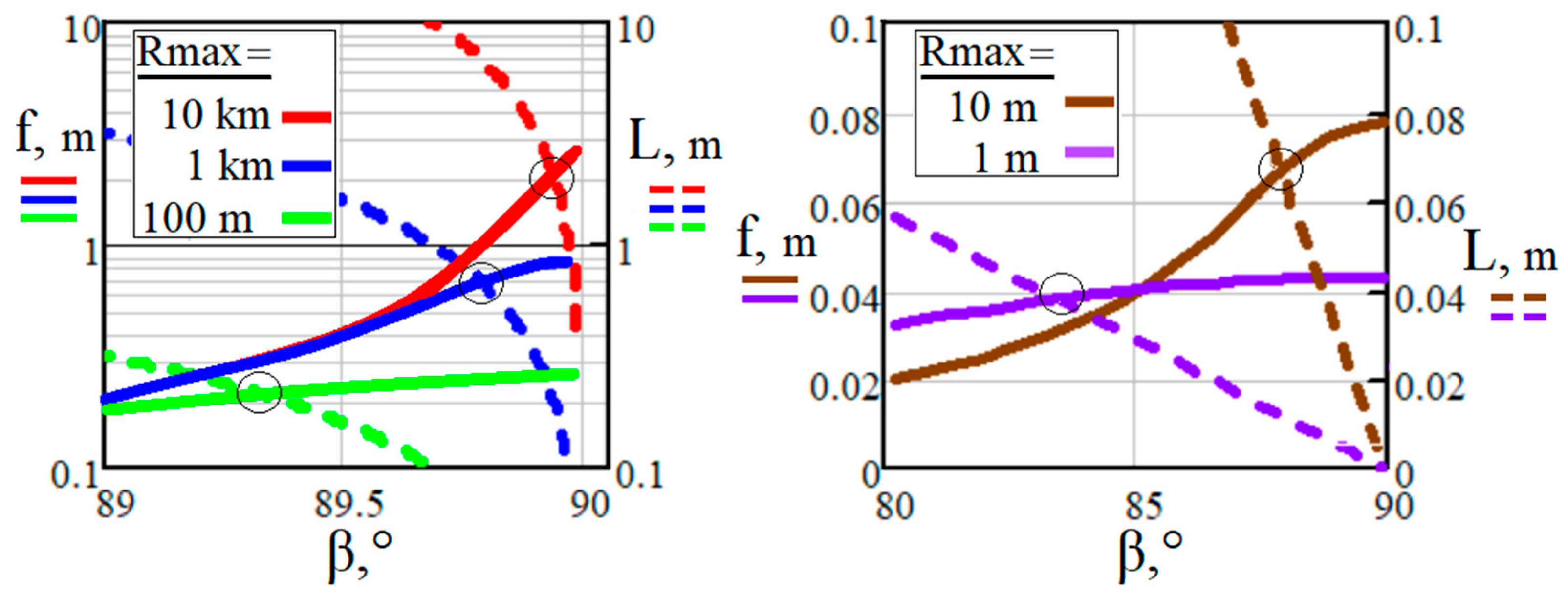
When α is preselected, changing angle β(α) according to (10) leads to the opposite trends in the corresponding changes in focal length f and lidar base L (Figure 6).
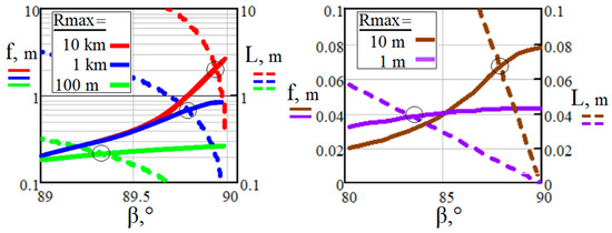
Figure 6.
Dependences of focal length f(β) and lidar base L(β) for Rmax = 10 km, 1 km, 0.1 km and 10 m, D = 10; Rmax = 1 m, D = 5; pΣ = 2 cm.
For example, the adjustments that increase angle β result in a focal length f increase, while the lidar base L decreases. The points of intersection of curves f(β) and L(β) circled in Figure 6 correspond to array tilt angles α ≃ π/4.
For a typical optical angle α = π/4, according to (12), . Given that M ≫ 1, we can write the following:
Then, the lidar base L and the distance Ldet to the array midpoint are equal:
Since it is always that M ≫ 1, according to (12) and (17), cotβ ≃ cosβ. If α = π/4, then it follows from (17) that
and given (18) and (19), the focal distance
Obviously, with the exception of tabletop prototypes, f = L is fulfilled with high accuracy.
2.3.2. Examples of S-Sensors Design to Achieve Different Dynamic Ranges D
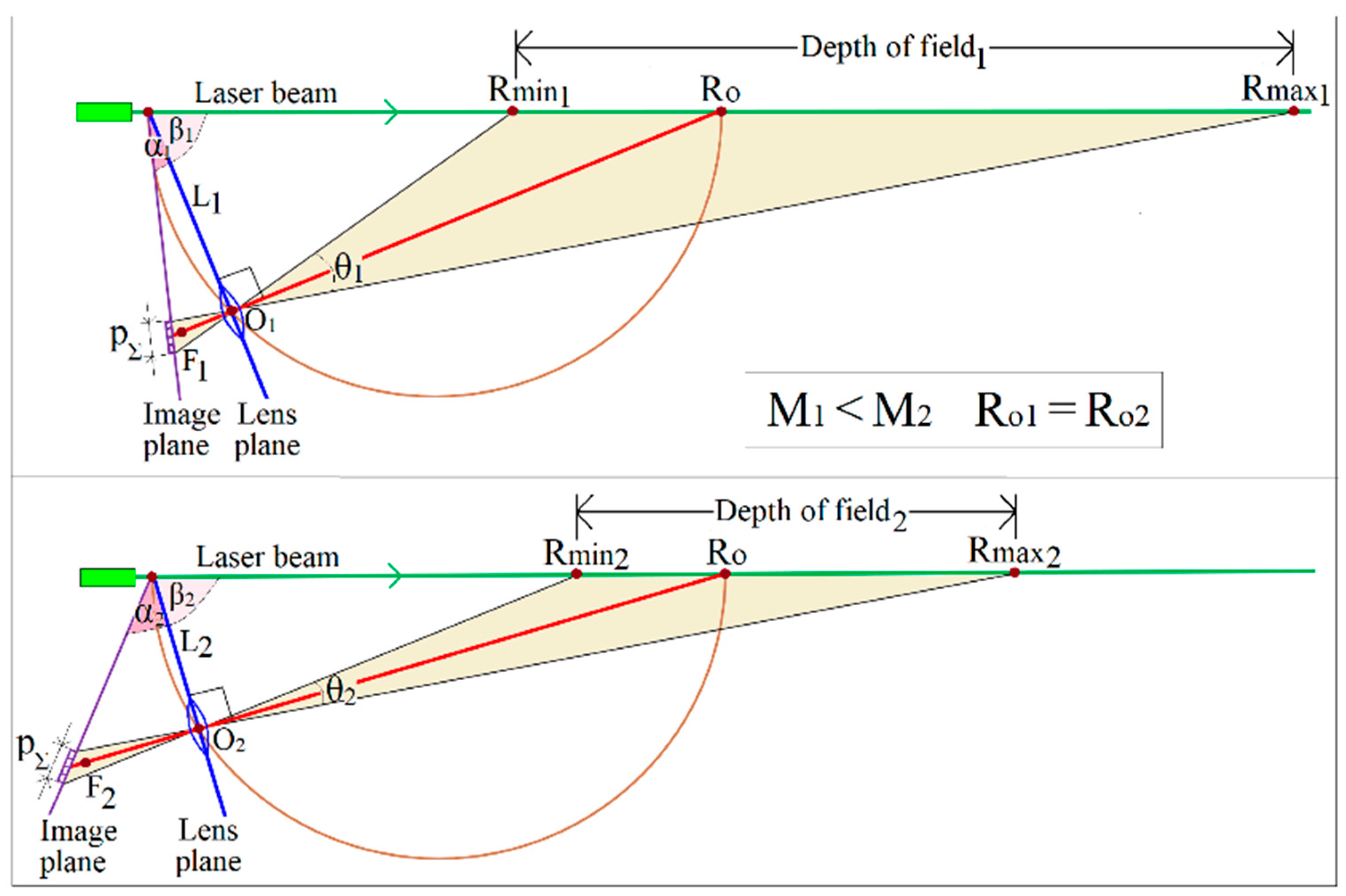
Let us consider the peculiarities of the choice of tilt angles α and β, lidar bases L and focal lengths f on the example of the comparison of two S-sensors, in which pΣ1 = pΣ2 = pΣ, Ro1 = Ro2 = Ro, and D1 > D2 (Figure 7).
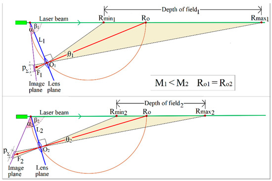
Figure 7.
Comparative geometry of two S-lidars with pΣ1 = pΣ2 = pΣ, Ro1 = Ro2 = Ro, and D1 > D2.
For a given Ro, the semicircle with diameter Ro is the universal geometrical locus of points for any S-lidar. Therefore, for any angles α and β, the receiving optical axis passes through the lens center, which must always be located on this semicircle. The receiving axis connects the point Ro with the lens center and continues to the linear array midpoint.
Let us show in the form of logical sequences how, for two S-lidar tools with the same pΣ and Ro, the differences in the required dynamic ranges (here D1 > D2) affect the ratios of focal lengths f1 and f2 and the corresponding bases L1 and L2. First, by virtue of (1)–(4) it turns out that
In addition, the condition tanα1 < tanα2 must be satisfied so that D1 > D2 at Ro1 = Ro2. On this basis, let us continue the logical sequence with respect to their tilt angles β1,2 and lidar bases L1,2:
D1 > D2 ⇨ β1 < β2 ⇨ L1 = R0·cosβ1 > L2 = R0·cosβ2 ⇨ L1 > L2
The logic of reasoning in regard to the required fields of view θΣ1,2 and focal lengths f1,2 with respect to α1 < α2 is as follows:
D1 > D2 ⇨ θΣ1 > θΣ2 ⇨ pΣ·cosα1/f1 > pΣ·cosα2/f2 ⇨ f1/f2 < cosα1/cosα2 > 1 ⇨ f1 < f2
Thus, the results of the qualitative comparison of parameters of the two sensors shown in Figure 7, can be presented in the form of Table 3.

Table 3.
Qualitative comparison of two S-sensors.
2.3.3. Receiving Field of View of S-Lidars: Adaptation to Depth of Field Required
To discuss the regularities, let us return briefly to Figure 2. The segment L is the base of the three triangles with vertices at points Rmin, Ro and Rmax and the angles at these vertices are equal, respectively, to γ0 + ½·θΣ, γ0 and γ0 − ½·θΣ. According to the already mentioned Law of Sines, the following relations are valid for these angles:
Hence,
The last expression is easily obtained, given that . Let us pay attention to a characteristic property of S-lidars; namely, adjustment range Ro of the receiving optical axis is determined only by the values of the depth-of-field borders Rmin and Rmax.
Therefore, dynamic range D = Rmax/Rmin is so related to the field-of-view (FoV) angle θΣ and the tilt angle γ0 of the receiving optical axis:
From this follows another important and universal relation characterizing S-lidars:
with a very simple conclusion: the interdependence of the FoV θΣ, and the receiving tilting angle γ0 is determined only by the required dynamic range D. In addition, the larger D is, the closer the field of view is to the doubled tilt angle of the receiving optical axis:
Since γ0 = π/2 − β, then for relatively small angles x
the flat field-of-view angle θΣ is defined from (29) as
If tilt angle α = π/4 as usual in optics is chosen, and based on (17), the effect of factor on the field of view can be described as (33) and is illustrated in Figure 8.
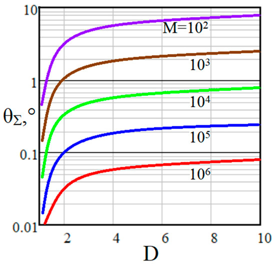
Figure 8.
Field of view θΣ of S-lidars as a function of dynamic range D at variations of M-index.
Note that the obtained analytical relations are of direct practical interest from another point of view. It is obvious that the external background caused by scattered solar radiation and perceived by the detector area gathers inside the solid angle formed by the receiver. Therefore, the desire to reduce the field of view in order to limit the external background is quite natural. In the case of the square shape of a single pixel, the power of perceived external background grows as the square of the flat FoV angle.
3. Results and Discussions
3.1. Achievable Range Resolution and Its Variability Bounds in S-Lidars
As we showed earlier [38], Equation (19), range resolution ΔR realized by S-lidars at an arbitrary distance R can be represented as
where we combined some characteristics of the receiving optics, lidar base and photodetector into such a cumulative parameter K1 [38], Equation (8).
with p1 as a single pixel size.
It follows from (34) and (35) that the larger the lidar base L and the smaller the field of view θ1, formed by a single pixel , the better the spatial resolution of S-lidars.
According to the left-hand side of (13) and using (15), the required lidar base and the focal length f of receiving optics for cotα ≫ cotβ were described. To predict the change in ∆Rmax ≡ ∆R(Rmax) analytically, substitute the above components into Equation (34) and obtain the following:
However, according to (8), the lens angle β depends on α and M as well as on Rmax and D inside M if we follow (3). Consider analytically only the common case of α = π/4 when S(π/4) = . Taking according to (17), Formula (36) is simplified to this form:
Given from (3) and , we can represent (37) as follows:
For large D ≫ 1, we can write as follows:
remembering that when comparing (39) with (38), the relative error δ < 10% already at D = 8 and decreases rapidly with increasing dynamic range D.
Before illustrating the result (38), let us recall that, envisaging a variety of applications of S-lidars, we consider a very wide operating range from a desktop prototype to multikilometer traces: Rmax = 1 m … 10 km. Along with this, the number of cells n of a linear array, as an example, can be in range n = 102 … 104. Consequently, the range of ratio ΔRmin = Rmax/n, characterizing the minimum possible range resolution under a very narrow range D → 1, turns out to be Rmax/n = 10−4 … 102 m.
The results of modeling range resolution ∆Rmax ≡ ∆R(Rmax) variability at the far border of DoF for α = π/4 are presented in Figure 9.
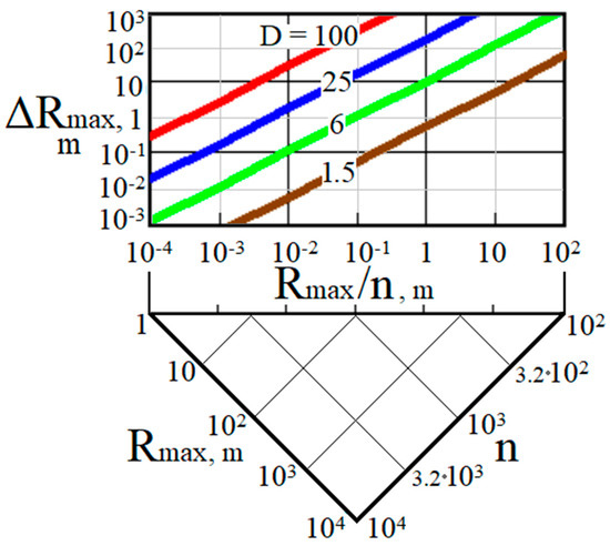
Figure 9.
Variability of range resolution ΔRmax at the far border Rmax of DoF; α = π/4.
It is easy to see that for any given ratio Rmax/n there is a very wide variability of the realized ΔRmax depending on the required value of dynamic range D = Rmax/Rmin. In addition, note that if instead of α = π/4 within the “one and a half” rule we choose arbitrary values of the tilt angle α, the right-hand sides of expressions (37)–(39) obtained from equation (36) should be multiplied by S(α)/S(π/4) according to (6).
3.2. Distant Far Border and Wide Dynamic Range Vs. High-Range Resolution: Achieving Acceptable Trade-Offs
3.2.1. Prerequisites for Further Application of the Q-Factor
Note that in many applications, system designers strive to provide both a wide depth-of-field (DoF) DR ≡ Rmax − Rmin = Rmax·(D − 1)/D and possibly higher-range resolution ΔR to have more detailed information about the object of study within the operation range. Let us return to the Q-index introduced in [38], assuming with its help to characterize the possibility of simultaneous achievement of both expectations. Following [38], for correct accounting of the S-lidar specificity (34), we will further control the index of its range–domain quality Q. It represents the ratio of the far border Rmax of DoF to the spatial resolution ΔR realized at this border ΔR(Rmax):
Obviously, this indicator, similar to quality index Q in the frequency domain and some others, is simple and very clear: the more, the better. When Rmax is fixed, the ability to increase Q means achieving better spatial resolution ΔR(Rmax). For a given ∆Rmax ≡ ∆R(Rmax), a larger value of Q characterizes the extended operating range.
The Q-factor is suitable when designing S-lidars having range-dependent spatial resolution, which distinguishes them from traditional pulsed and CW modulated lidars.
Indeed, since from (34)–(35), simple interdependencies follow from (40):
They describe possibilities of achieving quality Q = Rmax/ΔR(Rmax) at the minimum required value of K1 as a combined optical parameter of the transceiver.
Next, we show the advisability of an extended application of Q-factor to succinctly describe the relationship between cell number i and distance Ri to the i-th layer, potentially achievable length DR of the operation range, minimum required number nmin of the array cells, single cell size p1, dynamic range D, etc.
3.2.2. From i-th Pixel to i-th Layer at Distance Ri: A Simple Conversion Method
We showed earlier in [38], Equations (13) and (14), that the complex factor K0 = ½∙θΣ/γ0 = ½∙n∙R0/K1 with K1 = f∙L/(p1·cosα) and 0 < K0 ≤ 1 is one of collective parameters that can be useful in assessing the capabilities of S-lidar systems. Small values of K0 indicate a very narrow depth of field (DoF) centered around alignment range R0 of receiving optics. In addition, those close to 1 characterize the wide DoF. Its limiting value K0 = 1 refers to the so-called “infinite depth of field”, when the Rmax value tends to infinity.
Consideration of its interrelations can also be used to compactly describe the interdependence Ri = f(i).
When using S-lidars with array detectors, it is necessary to control the range to the i-th layer depending on the pixel number i. Instead of the ratios found in the literature [9,13,17,24,26], which are tied to the tilt angles and are not very convenient to use, we proposed another approach to their description. By numbering all pixels, i.e., assigning the i-th number to each pixel of the linear array, we apply the relation Ri = f(i) from [38], Equation (20), simplifying it somewhat:
where it is assumed that the conditions f/R0 ≪ 1 and K0 ∈ (0;1) are satisfied in the numerator (42). Here, R0 is the tuning range of the receiving optical axis; n is the number of cells of the linear array.
Let us reduce the equation to an even more convenient form on the basis of the following reasoning. According to [38], Equations (17) and (22), where (17), and (22), it can be written that
with K1 from (35). Equation (43) describes the S-lidar’s tuning range R0 as the point of intersection of the laser beam and the receiving optical axis. In a well-tuned receiving system, the last one passes through the midpoint of the array detector (i = n/2).
Substituting just mentioned parameters R0, K0 and K1 into (42), we obtain:
From this, we formulate another useful “rule” inherent only in S-lidars:
As can be seen, range Ri to the i-th layer can be easily predicted based on the system parameter K1 from (35), the number n of the array cells and the required value Q as a range–domain quality factor.
3.2.3. Formation of DoF as a Sequence of Spatially-Resolved Layers
Based on the result of (45), we write the current range resolution from Equation (34) as
Let us represent the depth of field (DoF) of sharply focused images as a sequence of spatially resolved layers ΔRi in range (Rmin; Rmax):
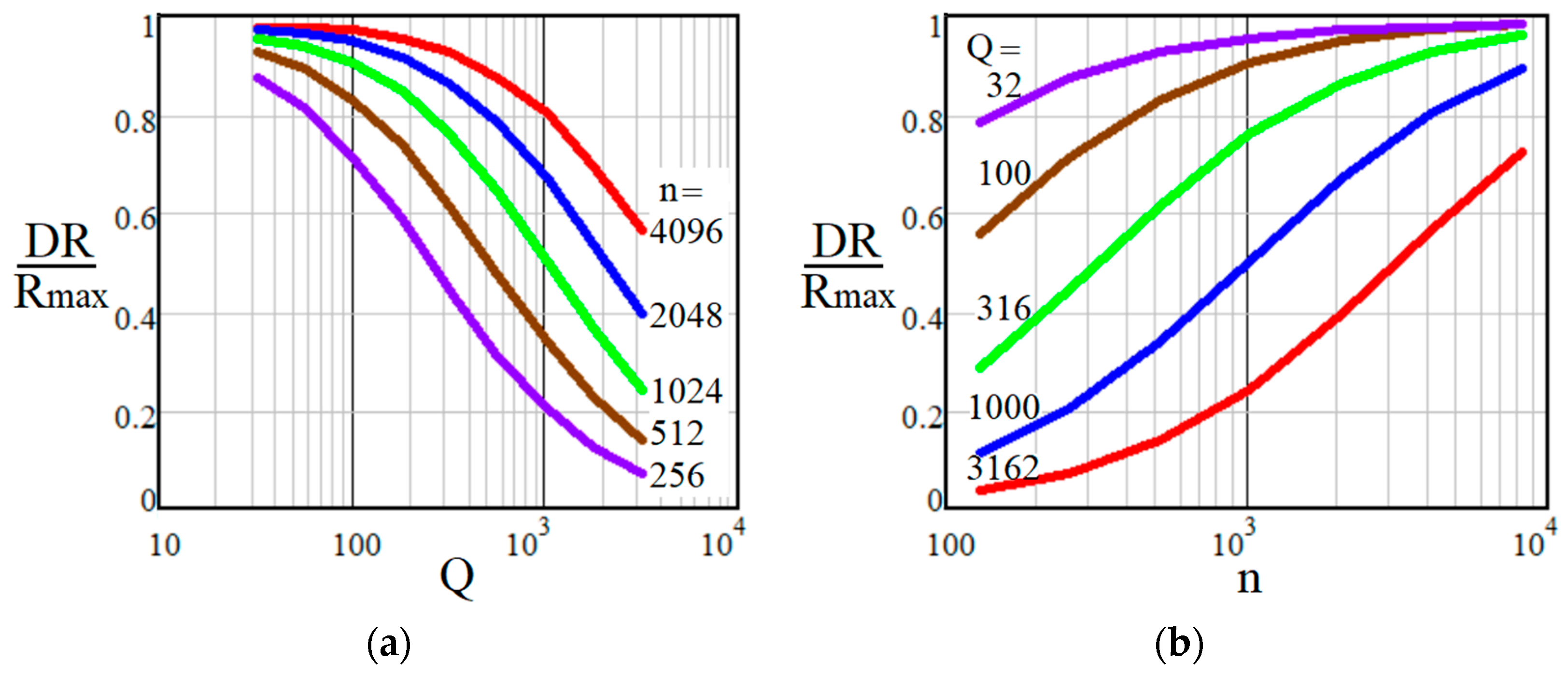
Figure 10 illustrates the variability of DoF normalized to Rmax = K1/Q.
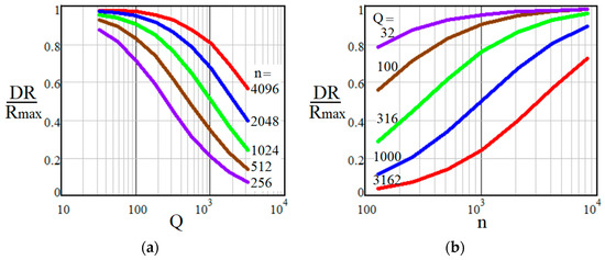
Figure 10.
Normalized variability of depth-of-field DR/Rmax as a function of Q-factor (a) and number of cells n (b).
The illustrated curves show that increasing range–domain quality requirements Q leads to a narrowing of the depth of field, while the arrays with a larger number n of cells allow the DoF to expand. Below, among other things, we will consider the cumulative effect of the Q and n parameters’ ratio Q/n.
3.2.4. Trade-Off between Wide Dynamic Range D and High Spatial Resolution ΔR(Rmax)
Let us describe the near border Rmin of the depth of field using (2), (41) and (44):
Hence, the minimum required number of cells n of a linear array capable of providing the condition R/ΔR(R) ≥ Q within the entire operation range DR = Rmax − Rmin is determined by two requirements: dynamic range D and range–domain quality Q
The required single pixel size p1 of a linear array detector of length pΣ should be no more than
If we use already available linear array p1 × n, the maximum achievable quality Q of remote sensing over a wide range D is limited by the following value:
which is illustrated in Table 4.

Table 4.
Maximum achievable range–domain quality index Q.
In other words, if an available linear array detector with n cells is used, the predicted dynamic range D = Rmax/Rmin, capable of providing range–domain quality R/ΔR(R) ≥ Q, is limited as follows:
Then, the achievable depth of field (DoF), taking into account (48) and (35), is
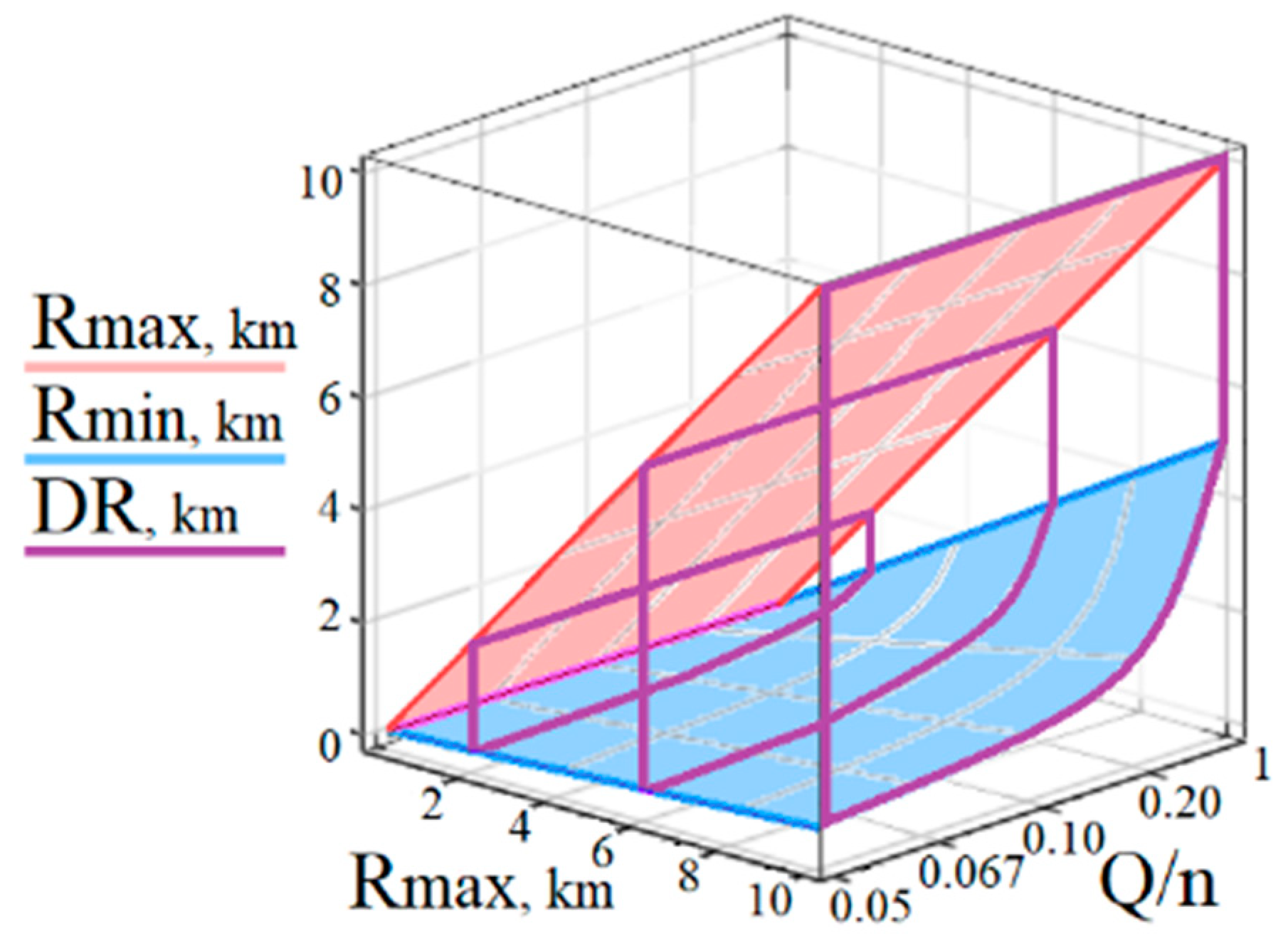
i.e., it is determined by the ratio between the required quality Q and the number of array cells n (Figure 11).

Figure 11.
Achievable depth-of-filed DR as a function of its far border Rmax and the Q/n ratio.
The DR width increases as n/Q grows (Q/n decreases), and the closer DR is to Rmax, the stronger the condition n/Q ≫ 1 is fulfilled.
Finally, based on the results of this study, Table 5 presents the predictions of CW RR S-lidars’ tactical and hardware parameters for various applications ranging from 1 m to 10 km.

Table 5.
Tactical and hardware parameters of S-lidars adapted for various applications and range scales.
We would like to point out that three estimates indicated in Table 5 by the symbol * should be seen as an expectation of new advances in nano- and microphoton technology.
4. Conclusions
We proposed a range–domain-oriented methodology for a generalized analysis of relationships between the non-energy parameters of S-lidars for a wide variety of applications and range scales, from desktop prototypes to a 10 km trace. Based on this analysis’s results, we synthesized the improved tools capable of smoothing out the contradiction inherent in S-sensors by finding a rational compromise in an attempt to simultaneously provide a wide dynamic range and high-range resolution. Scientific novelty of the problem statement, as well as our methods used and the results obtained, are predetermined by their application to S-lidars as a relatively new class of laser remote sensors with the nontraditional principles of design and operation. As a consequence, there was a need to revise typical ways of assessing their range–domain performance and received data interpretation. The focus of our research method is characterized by a dimensionless, parametric approach in order to take into account and compare the applications and tools of different scales with many interdependent and complementary parameters.
To set the desired far and near borders of the operating range, it was shown how to properly adjust the S-lidar by selecting the tilt angles of the lens plane and the image plane as well as the focal length, lidar base, etc. For this purpose, we introduced the mentioned dimensionless factors and criteria, including S-lidar-specific magnification M, angular function S, dynamic range D, “one and a half” condition, quality factor Q, efficiency factor Q/n, etc. This provided a high degree of generalization of analytical models for the use in a wide variety of cases. Finally, we demonstrated ways to achieve a compromise between the requirements for a wide dynamic range and high-range resolution. Possible limitations of the proposed approach with respect to the tilt angles and the receiving field of view were also discussed.
The results of the conducted analysis and synthesis allow increasing the validity of design solutions for further promotion of S-lidars for environmental remote sensing and their better adaptation to a broad spectrum of specific applications and range scales.
Author Contributions
Conceptualization and methodology, R.A.; investigation, R.A., Z.W. and D.L.; writing—review and editing, R.A.; resources and funding acquisition, Z.W. and D.L. All authors have read and agreed to the published version of the manuscript.
Funding
This research was funded by the Chinese Academy of Sciences (CAS-PIFI, 2023VEA0004), the National Natural Science Foundation of China (41975038), the Key Research and Development Program of Anhui Province (2022h11020008) and the HFIPS director’s Fund (2021YZGH01).
Institutional Review Board Statement
Not applicable.
Informed Consent Statement
Not applicable.
Data Availability Statement
No data were generated or analyzed in the presented research.
Conflicts of Interest
The authors declare no conflict of interest.
References
- Measures, R. Laser Remote Sensing: Fundamentals and Applications; Springer: Berlin/Heidelberg, Germany, 1984; p. 320. [Google Scholar]
- Fujii, T.; Fukuchi, T. Laser Remote Sensing; CRC Press: Boca Raton, FL, USA, 2005; p. 240. [Google Scholar]
- Rees, W. Physical Principles of Remote Sensing; Cambridge University Press: Cambridge, UK, 2006; p. 470. [Google Scholar]
- Agishev, R. Laser Remote Sensing of the Environment: Methods and Techniques; PhysMathLit-Press: Moscow, Russia, 2019; p. 264. [Google Scholar]
- McManamon, P. Lidar Technologies and Systems; SPIE-Press: Bellingham, WA, USA, 2019; p. 520. [Google Scholar]
- Ball, J.; Anderson, D.; Chan, C. Comprehensive survey of deep learning in remote sensing: Theories, tools, and challenges for the community. J. Appl. Remote Sens. 2017, 11, 42609. [Google Scholar] [CrossRef]
- Chen, R.; Li, Y.; Xue, G.; Tao, Y.; Li, X. Laser triangulation measurement system with Scheimpflug calibration based on the Monte Carlo optimization strategy. Opt. Express 2022, 30, 25290. [Google Scholar] [CrossRef] [PubMed]
- Xing, L.; Dai, W.; Zhang, Y. Scheimpflug camera-based technique for multi-point displacement monitoring of bridges. Sensors 2022, 22, 4093. [Google Scholar] [CrossRef] [PubMed]
- Yi, S.; Min, S. Composition of sharp-focused image by rotation of Scheimpflug camera. Opt. Laser Technol. 2022, 155, 108406. [Google Scholar] [CrossRef]
- Gao, F.; Lin, H.; Chen, K.; Chen, X.; He, S. Light-sheet based two-dimensional Scheimpflug lidar system for profile measurements. Opt. Express 2018, 26, 338056. [Google Scholar] [CrossRef]
- Chen, X.; Jiang, Y.; Yao, Q.; Ji, J.; Evans, J.; He, S. Inelastic hyperspectral Scheimpflug lidar for microalgae classification and quantification. Appl. Opt. 2021, 60, 4778–4786. [Google Scholar] [CrossRef]
- Lin, H.; Zhang, Y.; Mei, L. Fluorescence Scheimpflug lidar developed for the three-dimension profiling of plants. Opt. Express 2020, 28, 9269–9279. [Google Scholar] [CrossRef]
- Zhao, G.; Malmqvist, E.; Rydhmer, K.; Strand, A.; Bianco, G.; Hansson, L.; Svanberg, S.; Brydegaard, M. Inelastic hyperspectral lidar for aquatic ecosystems monitoring and landscape plant scanning test. EPJ Web Conf. 2018, 176, 01003. [Google Scholar] [CrossRef]
- Duan, Z.; Li, Y.; Wang, X.; Wang, J. Drone-based fluorescence lidar systems for vegetation and marine environment monitoring. EPJ Web Conf. 2020, 237, 07013. [Google Scholar] [CrossRef]
- Ma, X.; Wang, Z.; Zhang, H.; Shan, H.; Han, J.; Zhao, S.; Wang, S.; Liu, D.; Wang, Y.; Tao, Z. Detecting aerosol backscattering coefficient across the whole troposphere by the side-scattering lidar system with three CCD cameras. Opt. Express 2022, 30, 29969–29978. [Google Scholar] [CrossRef]
- Kong, Z.; Yu, J.; Gong, Z.; Hua, D. Visible, near-infrared dual-polarization lidar based on polarization cameras: System design, evaluation and atmospheric measurements. Opt. Express 2022, 30, 28514–28533. [Google Scholar] [CrossRef]
- Mei, L.; Brydegaard, M. Atmospheric aerosol monitoring by an elastic Scheimpflug lidar system. Opt. Express 2015, 23, A1613–A1628. [Google Scholar] [CrossRef] [PubMed]
- Liu, Z.; Li, L.; Li, H. Preliminary Studies on Atmospheric Monitoring by Employing a Portable Unmanned Mie-Scattering Scheimpflug Lidar System. Remote Sens. 2019, 11, 837. [Google Scholar] [CrossRef]
- Larsson, J.; Bood, J.; Xu, C. Atmospheric CO2 sensing using Scheimpflug-lidar based on a 1.57-µm fiber source. Opt. Express 2019, 27, 17348–17358. [Google Scholar] [CrossRef]
- Zhou, B.; Zhang, S.; Xue, R.; Li, J.; Wang, S. A review of space-air-ground integrated remote sensing techniques. J. Environ. Sci. 2021, 123, 3–14. [Google Scholar] [CrossRef]
- Yang, Y.; Guan, P.; Mei, L. A scanning Scheimpflug lidar system developed for urban pollution monitoring. EPJ Web Conf. 2018, 176, 01013. [Google Scholar] [CrossRef]
- Zhang, H.; Zhang, Y.; Li, Z.; Liu, B.; Yin, B.; Wu, S. Small angle scattering intensity measurement by an improved ocean Scheimpflug lidar system. Remote Sens. 2021, 13, 2390. [Google Scholar] [CrossRef]
- Duan, Z.; Yuan, Y.; Lu, J. Underwater spatially, spectrally, and temporally resolved optical monitoring of aquatic fauna. Opt. Express 2020, 28, 2600–2610. [Google Scholar] [CrossRef]
- Gao, F.; Li, J.; Lin, H. Oil pollution discrimination by an inelastic hyperspectral Scheimpflug lidar system. Opt. Express 2017, 25, 515–522. [Google Scholar] [CrossRef]
- Wang, X.; Duan, Z.; Brydegaard, M.; Svanberg, S.; Zhao, G. Drone-based area scanning of vegetation fluorescence height profiles using a miniaturized hyperspectral lidar system. Appl. Phys. A 2018, 124, 207. [Google Scholar] [CrossRef]
- Malmqvist, E.; Brydegaard, M.; Aldén, M.; Bood, J. Scheimpflug lidar for combustion diagnostics. Opt. Express 2018, 26, 14842–14858. [Google Scholar] [CrossRef]
- Rydhmer, K.; Prangsma, J.; Brydegaard, M.; Smith, H. Scheimpfug lidar range profiling of bee activity patterns and spatial distributions. Anim. Biotelemetry 2022, 10, 14. [Google Scholar] [CrossRef]
- Heyworth, G.; Knox, K.; Boydston, K.; Zhu, Y. Multispectral Scheimpflug: Imaging degraded books that open less than 30 degrees. Arch. Conf. 2022, 19, 1–4. [Google Scholar] [CrossRef]
- Agishev, R. Environmental CW range-resolved S-lidars with Si/InGaAs arrays: Limitations and capabilities under sky background. Appl. Opt. 2022, 61, 8889–8897. [Google Scholar] [CrossRef]
- Agishev, R. Application of Imaging S-lidars: Functional and Diagnostic Capabilities for Remote Air Pollution Detection. Opt. Eng. 2021, 60, 084104. [Google Scholar] [CrossRef]
- Scheimpflug, T. Improved Method and Apparatus for the Systematic Alteration or Distortion of Plane Pictures and Images by Means of Lenses and Mirrors for Photography and for Other Purposes. GB Patent 1904, GB190401196A, 2 February 1904. [Google Scholar]
- Carpenter, J. Improvements in Enlarging or Like Cameras. GB Patent 1901, GB190101139A, 2 November 1901. [Google Scholar]
- Meki, K. Range-resolved bistatic imaging lidar for the measurement of the lower atmosphere. Opt. Lett. 1996, 21, 1318–1320. [Google Scholar] [CrossRef] [PubMed]
- Barnes, J.; Bronner, S.; Beck, R.; Parikh, N. Boundary layer scattering measurements with a charge-coupled device camera lidar. Appl. Opt. 2003, 42, 2647–2652. [Google Scholar] [CrossRef]
- Cilingiroglu, U.; Chen, S.; Cilingiroglu, E. Range sensing with a Scheimpflug camera and a CMOS sensor/processor chip. IEEE Sens. J. 2004, 4, 36–44. [Google Scholar] [CrossRef]
- Steger, C. A comprehensive and versatile camera model for cameras with tilt lenses. Intl. J. Comput. Vis. 2017, 123, 121–159. [Google Scholar] [CrossRef]
- Sun, C.; Liu, H.; Jia, M.; Chen, S. Review of Calibration Methods for Scheimpflug Camera. J. Sens. 2018, 2018, 3901431. [Google Scholar] [CrossRef]
- Agishev, R. CW range-resolved S-lidars: Capabilities and limitations in range domain. Opt. Lasers Eng. 2020, 134, 106260. [Google Scholar] [CrossRef]
- Agishev, R. Imaging S-lidars enhancement by optimizing range-domain characteristics. Opt. Eng. 2021, 60, 034110. [Google Scholar] [CrossRef]
Disclaimer/Publisher’s Note: The statements, opinions and data contained in all publications are solely those of the individual author(s) and contributor(s) and not of MDPI and/or the editor(s). MDPI and/or the editor(s) disclaim responsibility for any injury to people or property resulting from any ideas, methods, instructions or products referred to in the content. |
© 2023 by the authors. Licensee MDPI, Basel, Switzerland. This article is an open access article distributed under the terms and conditions of the Creative Commons Attribution (CC BY) license (https://creativecommons.org/licenses/by/4.0/).


