Article

Cross-Domain Multi-Prototypes with Contradictory Structure Learning for Semi-Supervised Domain Adaptation Segmentation of Remote Sensing Images

PLA Strategic Support Force Information Engineering University, Zhengzhou 450001, China
*
Author to whom correspondence should be addressed.
Remote Sens. 2023, 15(13), 3398; https://doi.org/10.3390/rs15133398
Submission received: 11 May 2023 / Revised: 19 June 2023 / Accepted: 1 July 2023 / Published: 4 July 2023
(This article belongs to the Section Remote Sensing Image Processing)

Abstract

:
Recently, unsupervised domain adaptation (UDA) segmentation of remote sensing images (RSIs) has attracted a lot of attention. However, the performance of such methods still lags far behind that of their supervised counterparts. To this end, this paper focuses on a more practical yet under-investigated problem, semi-supervised domain adaptation (SSDA) segmentation of RSIs, to effectively improve the segmentation results of targeted RSIs with a few labeled samples. First, differently from the existing single-prototype mode, a novel cross-domain multi-prototype constraint is proposed, to deal with large inter-domain discrepancies and intra-domain variations. Specifically, each class is represented as a set of prototypes, so that multiple sets of prototypes corresponding to different classes can better model complex inter-class differences, while different prototypes within the same class can better describe the rich intra-class relations. Meanwhile, the multi-prototypes are calculated and updated jointly using source and target samples, which can effectively promote the utilization and fusion of the feature information in different domains. Second, a contradictory structure learning mechanism is designed to further improve the domain alignment, with an enveloping form. Third, self-supervised learning is adopted, to increase the number of target samples involved in prototype updating and domain adaptation training. Extensive experiments verified the effectiveness of the proposed method for two aspects: (1) Compared with the existing SSDA methods, the proposed method could effectively improve the segmentation performance by at least 7.38%, 4.80%, and 2.33% on the Vaihingen, Potsdam, and Urban datasets, respectively; (2) with only five labeled target samples available, the proposed method could significantly narrow the gap with its supervised counterparts, which was reduced to at least 4.04%, 6.04%, and 2.41% for the three RSIs.

1. Introduction

The continuous development of deep learning has given rise to a variety of methods with excellent segmentation performance, such as FCN [1], PSPNet [2], and UPerNet [3]. The introduction of these methods significantly boosts the performance of remote sensing image (RSI) semantic segmentation [4]. However, there are still two common shortcomings to these methods. On the one hand, the over-reliance on a large number of labeled samples greatly increases their application cost, because accurately labeling RSIs pixel by pixel is very time-consuming and labor-intensive [5]. On the other hand, considering the large discrepancies between different RSI domains in terms of resolution, image style, and so on, the widely used supervised learning (SL) mode, limited to a single domain, inevitably degrades their generalization ability [6,7]. Unsupervised domain adaptation (UDA), aiming to adapt the model trained on a labeled source domain to an unlabeled target domain, provides the possibility of alleviating the above problems. In recent years, there have been many explorations on UDA segmentation of RSIs, with some promising and instructive achievements [8]. The existing methods can be roughly divided into two categories: self-supervised-based methods and adversarial-based methods. Although the adopted learning modes and ideas are different, the above methods all attempt to improve the generalization performance of the models on target RSIs by reducing domain discrepancies [9]. However, it is indeed difficult to obtain accurate and satisfactory segmentation results only by utilizing unlabeled target samples to adapt to target RSI domains. According to the existing research, there is an obvious gap between the segmentation results of the UDA methods and those of their supervised counterparts, both qualitatively and quantitatively [10,11,12]. For example, the state-of-the-art entropy-guided UDA method for RSI segmentation [13] only obtained a pixel accuracy of 67.50% and a mean intersection over union of 47.29% on the Vaihingen dataset, and there were many recognition errors and a lot of noise in the obtained segmentation maps. Obviously, such segmentation results cannot provide accurate and reliable support for RSI intelligent interpretation, greatly reducing the practical application value of RSI domain adaptation segmentation.
Therefore, differently from the current mainstream UDA methods for RSI segmentation, this paper focuses on a more practical yet under-investigated problem, semi-supervised domain adaptation (SSDA) of RSIs. The intuitive idea behind this is to further improve the segmentation performance of target RSIs using a few labeled samples, which actually achieves a good trade-off between labeled samples and segmentation performance [14,15,16,17,18,19]. Compared with UDA methods, SSDA methods can bring a significant improvement; compared with supervised methods, the required number of labeled samples can be greatly reduced. Nevertheless, the existing studies have shown that the performance improvement brought by simply extending UDA methods to SSDA tasks is limited [14,15,17], and ideal results for target domains cannot be obtained, because the extension methods cannot fully integrate the feature information in source and target samples. Our experiments on domain adaptation segmentation of RSIs also reached similar conclusions. In the field of computer vision, research and methods tailored to the SSDA tasks have been developed in recent years. Through utilizing both abundant unlabeled samples and a few labeled samples in target domains, these SSDA methods can achieve better knowledge transfer and domain alignment than UDA methods, and thus significantly improve performance in domain adaptation tasks [19]. However, most of the existing research on SSDA focuses on the tasks of image classification and street scene segmentation [14,15,16,17,18,19]. Our experiments showed that directly applying the above methods cannot produce the desired results in the task of RSI domain adaptation segmentation, because they fail to fully fit the characteristics of the discrepancies between different RSI domains, such as different resolutions, changeable styles caused by imaging conditions and the spatial structure, and diverse instances within the same class.
In the SSDA segmentation of RSIs, the potential valuable information contained in the three different groups of samples, namely, abundant labeled source samples, abundant unlabeled target samples, and a few labeled target samples, should be fully mined and fused according to the characteristics of the RSIs, to further improve the segmentation results for the target RSIs. To this end, two considerations are proposed from the perspectives of prototype and feature alignment in this paper.
Multi-prototypes constraint across source and target domains. Due to the influence of sensors, imaging conditions, and other factors, there are obvious discrepancies between different RSI domains. Even in the same RSI domain, due to the wide coverage, the variances within the same class are worthy of concern. This paper revisits these problems from the perspective of prototypes, to alleviate the difficulties caused by them for RSI domain adaptations. The existing research on RSIs semantic segmentation usually learned one prototype for each class; actually, one feature vector that is expected to contain the representative information of the corresponding class [20]. However, considering the large inter-domain discrepancies and intra-domain variations, such methods are not sufficient to establish complex inter-class and intra-class relations. Taking the tree class and the building class as examples, Figure 1 shows their different instances in two RSI domains. As we can see, different instances of the same class have distinct characteristics in size, shape, texture, structure, and so on. Obviously, simply learning a single prototype for a given class cannot provide a unified abstract anchor for such diverse and disparate instances within that class. Therefore, we propose to represent each class as a set of prototypes. Different prototypes within the same class can model complex intra-class variances, while multiple sets of prototypes corresponding to different classes can better describe rich inter-class discrepancies. Furthermore, these prototypes are calculated and updated jointly using the three different groups of samples from source and target domains, to fully fuse rich feature information from different domains. The cooperative participation of source and target samples can actually constrain the two domains for implicit feature alignment. Therefore, maintaining multiple sets of prototypes with samples from different domains involves imposing cross-domain multi-prototype constraint for RSI domain adaptation.
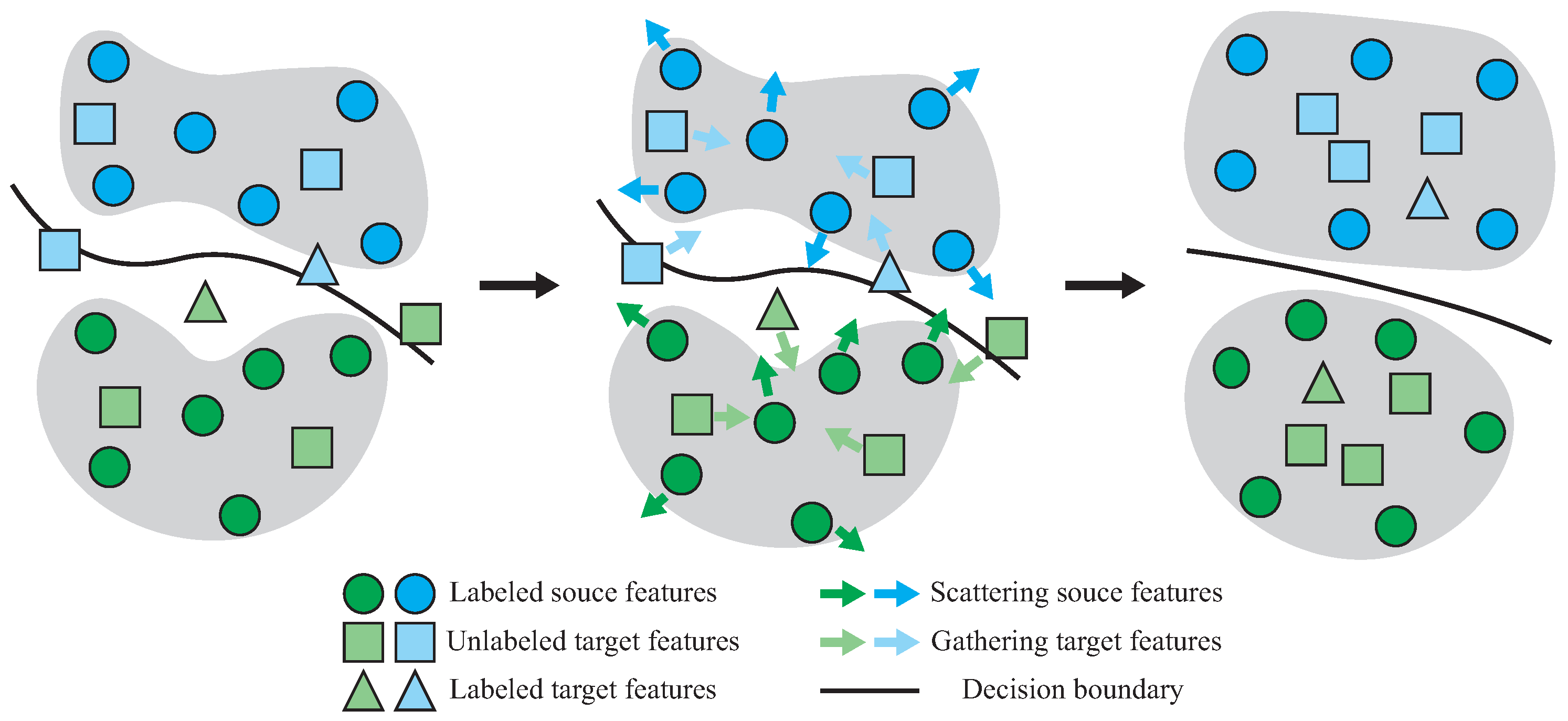
Improving feature alignment through contradictory structure learning. Due to the lack of labeled target samples, the number of target samples used for feature alignment is significantly less than that of the source samples, and even unlabeled target samples with high prediction probabilities are involved. Therefore, a contradictory structure learning mechanism is designed to explicitly improve the domain alignment. As vividly illuminated in Figure 2, the original features of the source and target domains are still not adequately aligned, and the individual feature points are outside the class cluster. Contradictory structure learning, on the one hand, gathers target features to increase the intra-class density and, on the other hand, scatters source features, to enhance the smoothness of the decision boundary. The goal is to make the target features, as much as possible, inside the dilated boundary of the source features, thus achieving a better domain alignment with an enveloping form and reducing misrecognition. In our work, contradictory structure learning is implemented using different feature fusion layers, attention mechanisms, and entropy functions.
In this paper, the above two approaches (multi-prototypes and contradictory structure learning) together with self-supervised learning are integrated into a unified framework, to improve the performance of RSI SSDA segmentation on the basis of fully utilizing and fusing the potentially valuable information in different domains. To sum up, the main contributions include the following four aspects:
(1)
A novel SSDA method for RSI semantic segmentation is proposed in this paper. To our knowledge, this is the first exploration of RSI SSDA, opening a new avenue for future work;
(2)
A cross-domain multi-prototype constraint for RSI SSDA is proposed. On the one hand, the multiple sets of prototypes can better describe intra-class variances and inter-class discrepancies; on the other hand, the cooperation of source and target samples can effectively promote the utilization of the feature information in different RSI domains;
(3)
A contradictory structure learning method is designed. Through gathering target features and scattering source features simultaneously, a better domain alignment with an enveloping form can be achieved;
(4)
Extensive experiments were carried out, and their statistics demonstrate that our method can, not only effectively improve the performance of SSDA segmentation of RSIs, but also significantly narrow the gap with supervised counterparts when only a few labeled target samples are available.

2. Related Work

2.1. RSI Semantic Segmentation

In recent years, deep learning methods have allowed remarkable achievements in RSI semantic segmentation [21,22]. A fully convolutional network (FCN) was the first model to demonstrate the powerful advantages of deep learning for semantic segmentation [1]. The Unet model adopted a more elaborate decoder and obtained better segmentation results, with fine-resolution [23]. Since then, a encoder–decoder structure has been widely adopted in RSs semantic segmentation, and a series of improved methods have been proposed. For example, Diakogiannis et al. introduced a residual connection and multi-task learning mechanism to enhance the fusion of features at different levels [24]. Liu et al. embedded self-cascaded convolution into a deep model, to improve the aggregation of semantic information at different scales [25]. Furthermore, to compensate for the limitation that convolution kernels cannot make full use of long-distance dependencies, attention mechanisms have begun to become popular. Ding et al. designed different attention modules for high-level and low-level features [26]. Li et al. developed a novel segmentation model based on multiple efficient attention modules, to fully utilize global contextual information [27]. Meanwhile, the performance of the transformer model for RSI semantic segmentation has also been widely explored [28], due to its excellent performance in natural image processing and analysis. He et al. embedded a Swin transformer into a Unet model, to make full use of global and local semantic information [29]. Wang et al. designed an advanced model based on a lightweight convolution model, transformer model, and attention mechanism, resulting in significant improvements in both segmentation accuracy and efficiency [30]. Meanwhile, research on instance segmentation [31,32] and small object segmentation [33] has also been developed and gained increased attention.
More recently, UDA methods were introduced, to improve the generalization performance of models on target RSI, by reducing domain discrepancies. Adversarial-based UDA methods can enable the generator to automatically learn domain-invariant features by jointly optimizing the generator and discriminator, and their performance in the RSI domain adaptation has been widely studied [34]. Chen et al. introduced a category-certainty attention module between the generator and classifier, to emphasize the importance of category-level alignment [35]. Chen et al. added a elevation estimation branch to the general UDA network, to improve the adaptation to target domains through multi-task learning [36]. However, it is undeniable that the process of adversarial training is a very challenging issue, due to the instability and difficulty of convergence [37]. In contrast, self-supervised-based UDA methods can effectively improve the segmentation results of target RSIs by fully utilizing pseudo-labels [38]. Wang et al. focused on the problem of spatial resolution inconsistency in RSI domain adaptation, effectively improving the effect of knowledge transfer from airborne to spaceborne images [39]. Yan et al. designed a cross teacher–student network and improved the classification results for target RSI through cross-consistency training [40]. In addition, style transfer [41] and image-to-image translation [42,43] methods were also introduced and combined with other UDA methods, to further improve the performance of RSI domain adaptation.
On the one hand, although a variety of UDA methods for RSI have been proposed, there is still a large gap between these and their supervised counterparts, according to the statistical results. On the other hand, the SSDA methods for RSI have been under-explored. To this end, this paper focuses on the SSDA segmentation of RSIs, to improve the segmentation performance for target RSIs with a few labeled target samples and to narrow the gap existing between UDA and supervised methods.

2.2. Semi-Supervised Domain Adaptation

Differently from UDA methods, SSDA methods can significantly improve the generalization and adaptation ability of a model to target domains using a few labeled samples [44]. The SSDA methods first appeared for the task of natural image classification and have gained attention and been further developed. Saito et al. proposed a novel minimax entropy method, to jointly optimize the encoder and classifier, and to learn domain-invariant features from source and target samples [14]. Li et al. effectively improved the classification accuracy of target domains by combining the advantages of categorical alignment, consistency alignment, and domain adaptation [15]. Yan et al. designed a multi-level consistency learning mechanism, to further improve the accuracy of SSDA classification [16]. At the same time, the SSDA methods tailored for street scene segmentation have also been proposed. For example, Wang et al. designed a semantic-level SSDA model, which significantly outperformed the state-of-the-art UDA models [17]. Alonso et al. achieved pixel-level contrastive learning through a designed memory bank updated with labeled samples, further improving the performance of SSDA segmentation on street scenes [18]. However, these methods fail to fully fit the characteristics of RSIs, and the results of directly applying these methods in RSI domain adaptation is not ideal.
Therefore, based on a full consideration of the discrepancies between different RSI domains, this paper proposes a novel SSDA method using the two aspects of prototypes and feature alignment. The proposed cross-domain multi-prototype constraint can achieve a better modeling of class-level relations on the basis of fully integrating the feature information of different domains. The designed contradictory structure learning module can achieve a better domain alignment with an enveloping form. The joint implementation of the two aspects can further improve the performance of SSDA segmentation of RSIs.

3. Methodology

3.1. Problem Setting

In the setting of SSDA, there are three different groups of samples: labeled source samples, labeled target samples, and unlabeled target samples. Formally, these can be denoted as S = { x i s , y i s } i = 1 N s , T = { x i t , y i t } i = 1 N t and U = { x i u } i = 1 N u , where x, y, and N represent samples, labels, and the size of datasets, respectively. The datasets S, T, and U actually share a common label space. There are abundant samples in S and U, while the number of available samples in T is very small; that is, N s N t and N u N t . Theoretically, it is certainly possible to train a model through supervised learning on S or T and perform segmentation on U. However, due to the large domain discrepancies between S and U and the imbalance in the number of samples between T and U, the above two approaches usually have a poor performance. In the domain adaptation setting, the dataset U can be further divided into U t and U v , where U t is used for domain adaptation training, while U v is used for evaluating the generalization performance of the trained model on target domains. There is no intersection between U t and U v . The SSDA methods aim to improve the segmentation accuracy of the model on U v through domain adaptation training on S, T, and U t .

3.2. Workflow

The workflow of the proposed method is presented in Figure 3. In terms of the model structure, the proposed method consists of a feature extraction module G, two different feature fusion modules F 1 and F 2 , a source scattering module H s , and a target gathering module H t . In terms of data flow, there are three different branches: labeled source samples, unlabeled target samples, and labeled target samples. An input sample is actually a RSI patch with a size of h × w × 3 . All the source and target samples are first mapped into deep feature vectors through the shared G and then input into the two feature fusion modules F. With the input of three different data flows, the modules F 1 will generate three groups of features, including labeled source features Z 1 s , unlabeled target features Z 1 u , and labeled target features Z 1 t . Correspondingly, the outputs of F 2 are denoted as Z 2 s , Z 2 u , and Z 2 t . Next, based on the above six groups of features, the model will perform cross-domain multi-prototype learning, contradictory structure learning, and self-supervised learning simultaneously.
Cross-domain multi-prototype learning. The above six groups of features are jointly responsible for cross-domain multi-prototype learning, which consists of online clustering and momentum updating. The former is to assign features to the different prototypes, while the latter is to update the prototypes according to the clustering results. In addition, it is worth noting that it is very important to determine the appropriate threshold for target pixels participating in multi-prototype updating, taking into account the fact that, if the threshold is too large, too many incorrect pseudo-labels will be used, damaging the learning effect; however, if the threshold is too small, the number of target pixels for multi-prototype learning will be greatly reduced, resulting in the bias of the obtained prototypes to source RSIs. The preliminary experiments showed that the proposed method achieved a better performance when the unlabeled pixels whose prediction probability was in the top 30% were used for prototype updating. With the cooperative participation of source and target samples, the generated cross-domain multi-prototypes contained rich feature information in different RSI domains. The segmentation results produced by online clustering and the corresponding labels are used to calculate the supervised loss L c e , which contains the loss of labeled source samples L s r c and the loss of labeled target samples L t a r . Meanwhile, the pixel-prototype contrastive loss L p p c and the pixel-prototype distance loss L p p d are added, to further optimize inter-cluster relation and enhance the intra-cluster compactness, respectively.
Contradictory structure learning. The process of contradictory structure learning is implemented using the four modules F 1 , F 2 , H s , and H t . During the backpropagation of L c e , the module F 1 receives ( 1 α ) L s r c + α L t a r and F 2 receives ( 1 α ) L t a r + α L s r c , where α [ 0 , 0.5 ) . Consequently, the modules F 1 and F 2 have different parameters and focus on the source and target RSI domains, respectively. The features Z 1 s , Z 2 t , and Z 2 u are first clustered based on the current prototypes. Then, the clustering results of Z 1 s are input to H s for source scattering, while the clustering results of Z 2 t and Z 2 u are input to H t for target gathering, and both sides work together to achieve a better domain alignment with an enveloping form.
Self-supervised learning. The predictions of the unlabeled target pixels with high probabilities can be used as pseudo-labels to further train the model. Specifically, the mean values of Z 1 u and Z 2 u , i.e., ( Z u = ( Z 1 u + Z 2 u ) / 2 ) , are taken as the deep features for self-supervised learning, to fully combine the different strengths of F 1 and F 2 . Then, the pseudo-labels obtained by the nearest prototype retrieving Z u and the corresponding samples are used to generate the new sample-label pairs for self-supervised training through data augmentations, such as rotation, crop, and color jitter.
The cross-domain multi-prototypes and contradictory structure learning are the main innovations in the proposed method, while the self-supervised learning can provide high-quality pseudo-labels and effectively increase the number of target samples involved in multi-prototype updating and domain adaptation training. Through combining these different advantages, the proposed method can fully mine and utilize the feature information in the three different groups of samples, to effectively improve the adaptation and transfer to target RSI domains.

3.3. Cross-Domain Multi-Prototype Constraint

3.3.1. Multi-Prototype-Based Segmentation

Given an input RSI patch denoted as I R h × w × 3 , the modules G and F first map this to the feature vector Z R H × W × D . For the segmentation task with C classes, the label of each pixel is determined with reference to the C sets of prototypes, where each set contains K prototypes. Specifically, the prototypes can be denoted as P = { p c , k R D } c , k = 1 C , K , in which each prototype is determined as the center of a k-th subcluster of features belonging to the c-th class. The class prediction of each pixel is achieved through nearest prototype retrieval [45]:
c ^ z = c * , with ( c * , k * ) = argmin ( c , k ) { z , p c , k } c , k = 1 C , K ,
where z R D is the feature after L2 normalization, and the distance measure · , · is defined as the negative cosine similarity. Furthermore, based on the prediction obtained using Equation (1) and the groundtruth label c z { 1 , d o t s , C } , the cross entropy loss is calculated:
L c e = log p ( c z z ) = log exp ( s z , c z ) exp ( s z , c z ) + c c z exp ( s z , c ) ,
where p ( c z ) is the probability distribution of the feature z over C classes, and s z , c = m i n { z , p c , k } k = 1 K is the distance between the feature and the closet prototype of class c. As illustrated in Figure 4a, the Equation (2), on the one hand, can push the embedded pixel closer to the nearest prototype of its corresponding class c z ; on the other hand, it can pull it away from other close prototypes of irrelevant classes, i.e., c c z .

3.3.2. Online Clustering and Momentum Updating

The entire process of online clustering and momentum updating can be summarized as follows: the features within the same class are assigned to multiple prototypes belonging to that class, and then the current prototypes are updated based on this assignment. Formally, given the three different groups of samples from the source and target RSI domains in a batch, the features Z c = { z n } n = 1 N are first generated, where N = H × W . The goal of online clustering is to assign the features Z c to the K prototypes { p c , k } k = 1 K belonging to the class c. This assignment process can be denoted as L c = [ l z n ] n = 1 N , where l z n = [ l z n , k ] k = 1 K { 0 , 1 } K is the one-hot vector assigning features z n to the K prototypes. The probability matrix L c can be optimized by maximizing the similarity between the features Z c and prototypes P c :
max Tr L c ( L c P c Z c ) , s . t . L c { 0 , 1 } K × N , L c 1 K = 1 N , L c 1 N = N K 1 K ,
where 1 N is the vector with N-dimension elements that are all ones. The constraint L c 1 K = 1 N ensures that each feature can only be assigned to one prototype. The constraint L c 1 N = N K 1 K ensures that each prototype can be selected at least N / K times in a batch on average, which can effectively prevent the model from being optimized to extreme or trivial solutions, such as assigning all features to a single prototype.
The solution of Equation (3) can be completed by relaxing L c to be an element of the transportation polytope:
max Tr L c ( L c P c Z c ) + κ h ( L c ) s . t . L c R + K × N , L c 1 K = 1 N , L c 1 N = N K 1 K ,
where κ > 0 is the hyperparameter controlling the smoothness of distribution and h ( L c ) = n , k l z n , k log l z n , k is the entropy. Furthermore, the solver of Equation (4) can be given based on the soft assignment relaxation and the regularization term h ( L c ) :
L c = diag ( u ) exp ( P c Z c ) κ ) diag ( v ) ,
where u R K and v R N are renormalization vectors computed using a few steps of Sinkhorn–Knopp iteration [46].
Obviously, the prototypes are constructed directly on the input samples themselves, without introducing additional parameters that need to be optimized. More specifically, the prototypes are actually calculated as the centers of the corresponding features. Therefore, the prototypes can be continuously updated by taking full account of the online clustering results:
p c , k μ p c , k + ( 1 μ ) z ¯ c , k ,
where μ [ 0 , 1 ] is the coefficient for momentum updating, and z ¯ c , k represents the mean vector of features after L2 normalization.

3.3.3. Contrastive Learning and Distance Optimization

There are two main deficiencies in Equation (2). First, the inter-cluster relation is not clearly expressed. In other words, the embedded pixels should be pushed closer to a certain prototype and relatively away from other prototypes within the same class (illustrated in Figure 4b). Second, Equation (2) cannot directly regularize the distances between the embedded pixels and classes. This may make the large intra-class distance only produce a small penalty loss, because the intra-class distance may be smaller, relatively, than the inter-class distance [47]. However, the embedded pixels should be more tightly distributed around the corresponding prototype, to improve the compactness and discriminability of the different clusters (illustrated in Figure 4c). Therefore, pixel-prototype contrastive loss and pixel-prototype distance loss are introduced to deal with the above two problems, respectively.
During online clustering, pixel-prototype contrastive learning is implemented by maximizing the prototype assignment posterior probability:
L p p c = log exp ( z p c z , k z / τ ) exp ( z p c z , k z / τ ) + p P exp ( z p / τ ) , s . t . k z = argmax k { l z , k } k = 1 K , l i , k l z ,
where P = { p c , k } c , k = 1 C , K / p c z , k z , the hyperparameter τ is used for controlling the concentration level, and k z indexes the prototypes belonging to class c. Intuitively, the Equation (7) can reduce the distance between each feature and its assigned prototype p c z , k z (positive prototype) and increase the distance between each feature and other C K 1 prototypes P (negative prototypes) belonging to the same class.
Meanwhile, the pixel-prototype distance loss is calculated as follows:
L p p d = ( 1 z p c z , k z ) 2 ,
where both the z and p c z , k z are L2 normalized. The objective of Equation (8) is to minimize the distance between each feature and its assigned prototype, which can effectively reduce the intra-cluster variation.
During the whole process of prototype clustering and updating, the total loss is defined as
L p r o = L c e + λ 1 L p p c + λ 2 L p p d ,
where λ 1 and λ 2 are weight coefficients. In summary, the losses L c e , L p p c and L p p d can optimize the learning process from three different levels of inter-class relation, inter-cluster relation, and intra-cluster compactness. Figure 4 gives a visual explanation. Consequently, clustering different embedded pixels around different prototypes can better model inter- and intra-class relations. This is very important and effective for RSI domain adaptation, since multiple instances of a class are very distinct from each other in different domains. In addition, the joint participation of source and target samples is the data basis for giving full play to the advantages of the cross-domain multi-prototypes. Only in this way can the generated prototypes better aggregate and fuse the feature information of different RSI domains.

3.4. Contradictory Structure Learning

In this section, the specific process of contradictory structure learning in H s and H t is described in detail. On the one hand, existing research has shown that the entropy function can effectively measure the closeness of features [14,48]; on the other hand, the adoption of an attention mechanism can further enhance the focus on important and discriminative features. Therefore, the modules H s and H t are designed as a combination of an attention mechanism and entropy function.
According to Equations (3)–(5), the clustering results are actually vectors that can be denoted as O = { o n } n = 1 N R N × C . Taking the module H t as an example, the vectors first pass through the attention module and then are used to compute the entropy function. Specifically, the advanced attention mechanism ACmix [49] is adopted, due to its ability to integrate the different advantages of convolution and self attention. Figure 5 briefly shows its workflow, which can be divided into three steps. First, the input vectors are projected using 1 × 1 convolutions to generate rich intermediate features. Next, the generated features are input into the self-attention branch and the convolution branch, and the different strengths of each branch are used for feature information selection and aggregation. Finally, the outputs of the two branches are combined to generate the transformed feature vectors, which can be denoted as A = { a n } n = 1 N R N × C .
As shown in Figure 3, the module H t clusters both label target samples and unlabeled samples. In a batch, their corresponding features can be denoted as a t and a u , respectively, and the union set of the two can be denoted as a u t . Therefore, the conditional entropy loss in H t is calculated:
L h t = E a u t A u t [ c = 1 C p ( y = c a u t ) log p ( y = c a u t ) ] ,
where y includes the truth labels and the pseudo-labels corresponding to the features a t and a u . The optimization of Equation (10) can effectively cluster target features by enforcing the high-confidence predictions.
Similarly, taking the clustering results of source features as the input, the module H s first utilizes the attention mechanism ACmix for feature aggregation and then computes the entropy loss. By analogy, scattering features can be regarded as the inverse process of clustering features. Similarly to the module H t , the loss function in the modules H s can be calculated:
L h s = E a s A s [ c = 1 C p ( y = c a s ) log p ( y = c a s ) ] ,
where a s represents the features of the labeled source samples in a batch. Therefore, in the whole process of contradictory structure learning, the total loss can be denoted as
L c s l = β ( L h t + L h s ) ,
where β is the weight coefficient. The loss functions L h t and L h s can prompt the modules H t and H s to cluster target samples and scatter source samples, respectively, thus achieving better feature alignment with an enveloping form between different RSI domains.

3.5. Optimization Objective

Before the overall optimization objective is given, the calculation process of self-supervised loss is formalized, as follows: The features of the augmented unlabeled samples generated by F 1 and F 2 are denoted as z 1 u and z 2 u , respectively, and the mean features, i.e., z u = ( z 1 u + z 2 u ) / 2 , are used for class prediction. Therefore, the self-supervised loss is calculated:
L s s l = log exp ( s z u , c z u ) exp ( s z u , c z u ) + c c z u exp ( s z u , c ) .
Furthermore, the overall optimization objective of the proposed method can be summarized as
L a l l = L p r o + L c s l + L s s l ,
where the losses L p r o , L c s l , and L s s l correspond to the three different learning mechanisms. By integrating their different advantages, the proposed method can fully mine and fuse the feature information in the source and target samples, effectively improving the performance of RSI SSDA segmentation. In addition, Algorithm 1 summarizes the pseudo-code, to clearly show the entire workflow of the proposed method.
Algorithm 1 Proposed SSDA method for RSI segmentation
Require: 
Labeled source RSI samples I s
Require: 
Labeled target RSI samples I t , unlabeled target RSI samples I u
  1:
Randomly initialize different modules G, F 1 , F 2 , H s , H t
  2:
Randomly initialize prototypes P
  3:
while not done do
  4:
  Generate features Z 1 s , Z 1 u , Z 1 t , Z 2 s , Z 2 u and Z 2 t
  5:
  Calculate L p r o with Equation (9)
  6:
  Calculate L c s l with Equation (12)
  7:
  Calculate L s s l with Equation (13)
  8:
  Calculate L a l l with Equation (14)
  9:
  Update P
  10:
   Update G, F 1 , F 2 , H s , H t
  11:
end while

4. Experimental Results

4.1. Dataset Description

Three RSI datasets, Vaihingen (VH), Potsdam (PD), and LoveDA, [12] were used for the experiments, and their details are listed in Table 1. The VH dataset contains 33 images, which are divided into two groups consisting of 16 images and 17 images, respectively, according to the official statements. The PD dataset consists of 38 images, which are divided into two groups consisting of 24 images and 14 images, respectively. Both these two datasets contain the same six classes: impervious surface, building, low vegetation, tree, car, and cluster. During preprocessing, all images were cropped to samples with 512 × 512 pixels. Consequently, the VH dataset produced 344 and 398 samples, respectively, while the PD dataset produced 3456 and 2016 samples, respectively.
Compared with the above two datasets, LoveDA is a more challenging spaceborne RSI dataset. It contains seven classes: background, building, road, water, barren, forest, and agricultural. The dataset is divided into two domains: rural and urban. The rural domain contains 1366 training images and 992 validation images, and the urban domain contains 1156 training images and 677 validation images. Each image is 1024 × 1024 pixels.
Referring to [13,50], three SSDA segmentation tasks, PD→VH, VH→PD, and Rural→Urban were designed. Table 2 summarizes the different task settings. Taking the first task as an example, the 3456 labeled samples of the PD dataset, the 398 samples of the VH dataset without labels, and the 5 labeled samples selected from the 398 samples were used for domain adaptation training, while the 344 samples of the VH dataset were used for evaluation.

4.2. Experimental Settings

The hardware environment includes a computer equipped with an Intel Xeon Gold 6152 CPU and an Nvidia A100 PCIE GPU. The software environment was developed using the ubuntu system, including Python 3.9 and machine learning libraries.
Referring to [11,13,34], the widely used DeepLabv2 segmentation framework with the ResNet-101 model was adopted. The module G was actually the ResNet-101 model pretrained on the ImageNet dataset, without the last pooling layer and fully connected layer. The modules F 1 and F 2 had the same structure, i.e., the improved atrous spatial pyramid pooling module, which were responsible for fully extracting and utilizing the features at different scales. Specifically, the number of input channels was 2048, and the dilated rates were 6, 12, 18, and 24. The modules H s and H t were developed based on ACmix and also had the same structure. The three 1 × 1 convolutions first projected the input vector to 18 intermediate feature maps. Then, the multi-head self attention mechanism with 3 heads was used for feature aggregation in the self-attention branch, and the fully connected layer and 3 × 3 two-dimensional convolutions were adopted to shift and aggregate features in the convolution branch.
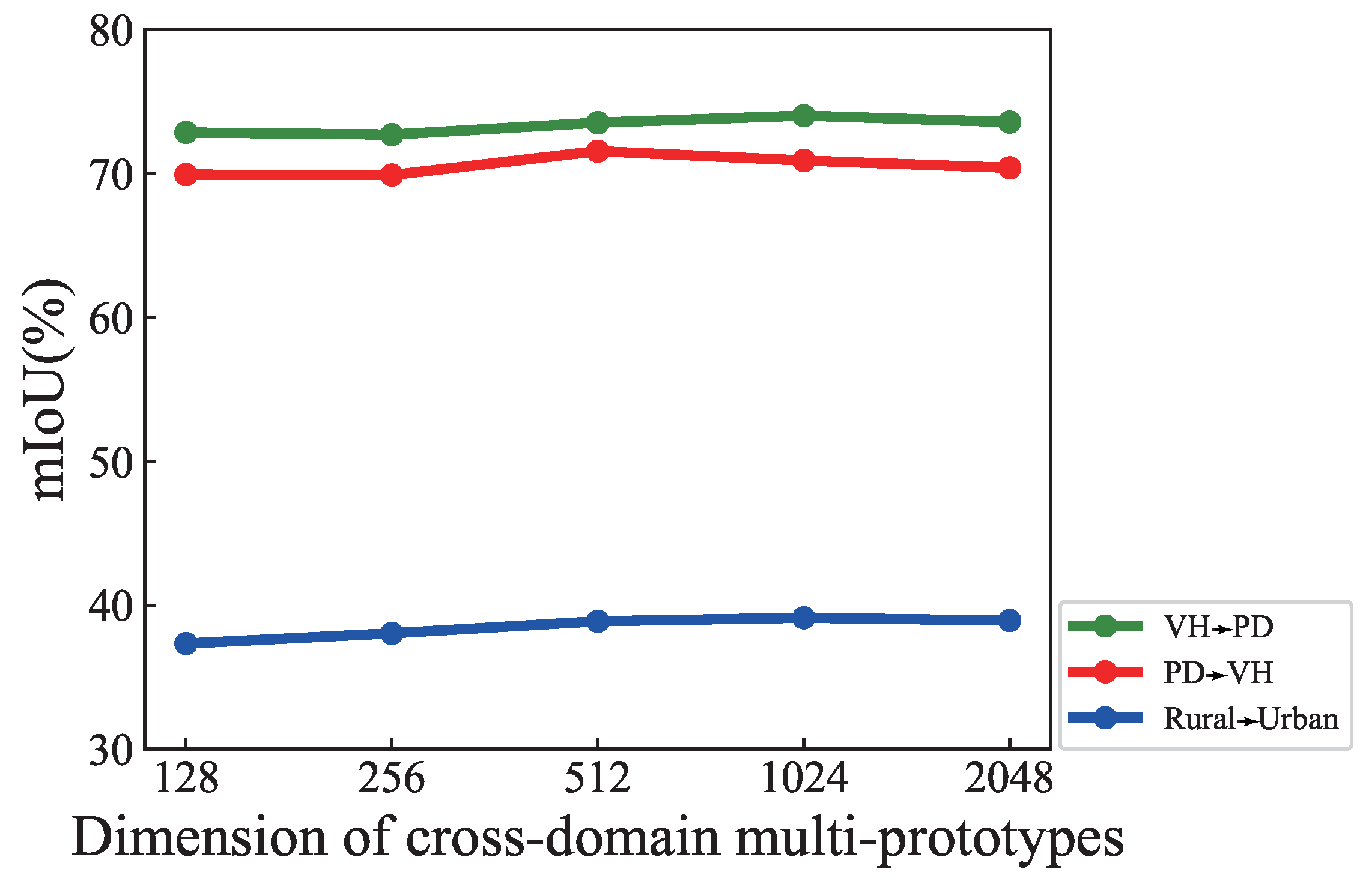
The selection of hyperparameters was mainly based on relevant research or experimental results. During domain adaptation training, the number of prototypes per class was 20, and the dimensions of prototypes were set to 512 for the first task, and 1024 for the other two tasks (analyzed in Section 5.3). According to existing research, compared with the Adam and SGD optimizers, the AdamW algorithm enables deep models to achieve faster convergence and better performance, and it has been widely used in many tasks [51]. Therefore, the AdamW algorithm was used for parameter optimization, where the hyperparameters β 1 and β 1 were set to 0.9 and 0.999, respectively, and the weight decay coefficient was 0.01. The coefficient β was set to 0.1. Referring to [45,48], the weight coefficients λ 1 , λ 2 , and μ were set to 0.01, 0.001, and 0.999, respectively. The hyperparameter α was 0.25, ensuring that the modules F 1 and F 2 focused on the source and target domains, respectively. The learning rate of G was 0.0001, while the learning rates of F 1 , F 2 , A 1 , and A 2 were all set to 0.001, for a faster convergence. In addition, the poly decay strategy was applied for a more adequate training. The maximum number of iterations was set to 20,000 and the batchsize was 4, which means that there were 4 labeled source samples, 4 unlabeled target samples, and 4 labeled target samples in each iteration. To ensure the quality of the pseudo-labels, self-supervised learning was carried out after 2000 iterations, and the pixels whose prediction probability was in the top 30% were used for prototype updating.
Referring to [11,26,36], the pixel accuracy (PA), intersection over union (IoU) per class, and mean value of IoU (mIoU) were used to quantitatively evaluate the segmentation performance of the different methods on the target RSIs.

4.3. Quantitative Results and Comparison

In this section, five SL methods, six UDA methods, and seven SSDA methods were used for quantitative comparison, to verify the effectiveness of the proposed method from two aspects: (1) Comparing the performance of the proposed method and existing SSDA methods in semi-supervised domain adaptation segmentation of RSIs; (2) Analyzing the ability of the proposed method to bridge the gap with the SL methods in the segmentation results of target RSIs.

4.3.1. Comparison with SSDA Methods

First, the superiority of the proposed method in improving the performance of RSI semi-supervised domain adaptation segmentation was analyzed. The SSDA methods for quantitative comparison were as follows: (1) DACS (SSDA). The UDA method DACS is a cross-domain mixed sampling method based on self-supervised learning [52], which was extended to the SSDA tasks by inputting a few labeled target samples into the student network for supervised training and sample mixing. (2) Zheng’s (SSDA). The Zheng UDA method is an advanced entropy guided adversarial learning algorithm with local feature alignment and graph convolutions for RSI UDA segmentation [13], which was extended to a SSDA method through adding a few labeled target samples into the supervised segmentation flow. (3) RDG (SSDA). The UDA method RDG is an advanced RSI-to-RSI translation method, focusing on scale discrepancy and translation stability [42], which was also extended to a SSDA method by incorporating supervised training on a few labeled target samples into the domain adaptation process. (4) MME. A classic SSDA method that can adversarially optimize models via a minimax entropy strategy [14]. (5) CDAC. A cross-domain adaptation clustering method aiming to achieve both inter- and intra-domain adaptation [15]. (6) Alonso’s. A SSDA method designed for street scene segmentation, which can perform pixel-level contrastive learning via a class-wise memory bank [18]. (7) Hoyer’s. An advanced SSDA method that can effectively enhance the segmentation results of target images through self-supervised monocular depth estimation.
All the methods and the proposed method followed the settings in Table 2, and the statistical results are listed in Table 3 and Table 4, which can be summarized into the following four aspects:
(1)
The improvement in the segmentation performance for the target RSIs brought by the three extension SSDA methods was limited compared with the corresponding UDA methods. For example, the mIoU of Zheng’s (SSDA) in the three tasks increased by only 0.48%, 3.03%, and 0.90%, respectively. This indicates that simply extending the UDA methods to SSDA methods cannot obtain ideal results in SSDA segmentation of RSIs;
(2)
The two methods MME and CDAC could improve the segmentation performance for the target RSIs to a certain extent, and the mIoU increased by about 3.9%, 1.5%, and 0.3% on average, respectively, in the three tasks, compared with the three extension SSDA methods. In addition, the adaptive clustering strategy endowed CDAC with a better generalization ability, so its segmentation results were better than those of MME. However, both methods were originally designed for SSDA classification of natural images and are not suitable for dense prediction, so there is still a lot of room for performance improvement;
(3)
The two advanced SSDA methods for semantic segmentation, Alonso’s and Hoyer’s, could effectively improve the segmentation results by a large margin. Compared with CDAC, the mIoU of Alonso’s increased by 7.23%, 18.47%, and 1.28% in the three tasks, respectively, while the mIoU of Hoyer’s increased by 9.89%, 20.88%, and 2.83%, respectively. The network structures designed for semantic segmentation and advanced strategies tailored to SSDA enabled the two methods to better adapt to and generalize for the target RSIs;
(4)
The proposed method achieved the best segmentation results among all the SSDA methods, both in terms of overall metrics and individual classes. In the first task, the mIoU and PA of the proposed method were 7.38% and 4.41%,respectively, higher than those of the second-place method. In the second task, the mIoU and PA of the proposed method were 4.80% and 2.48%,respectively, higher than those of the second-place method. In the third task, the mIoU and PA of the proposed method were 2.33% and 1.49%, respectively, higher than those of the second-place method. Such improvements benefited from the ability of the proposed method to fully extract, fuse, and align the feature information in the source and target samples. Specifically, the representation abilities of multi-prototypes for inter- and intra-class relations, and the better domain alignment with an enveloping form, enabled the proposed method to better distinguish the classes with high inter-class similarity. For example, in the second task, the proposed method improved the IoU of the classes low vegetation and tree by 2.36% and 3.28%, respectively, compared with the second-place method. Meanwhile, the segmentation performance for challenging classes that were difficult to identify using the other methods was also greatly improved. For example, the proposed method increased the IoU of the car class by 11.13% and 14.19%, respectively, in the first two tasks, and increased the IoU of the agriculture class by 2.61% in the third task, over the second-place method.
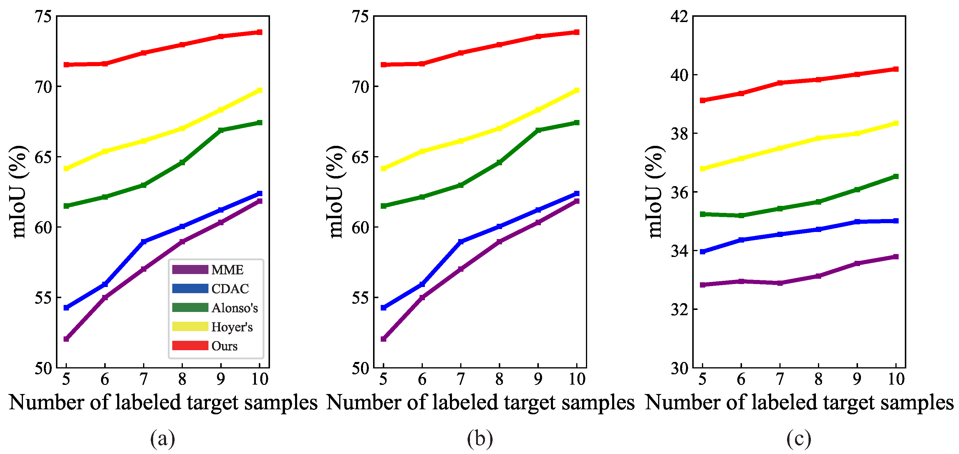
The comparison results of the SSDA methods and proposed method with a different number of labeled target samples are shown in Figure 6. As we can see, when the number of labeled target samples was increased from 5 to 10, the mIoU of all methods increased gradually. Obviously, more annotation information would be beneficial to further improve the segmentation results for the target RSIs. The curve corresponding to the proposed method was always above the other curves, indicating that the proposed method had advantages over the existing SSDA methods in the SSDA segmentation of RSIs.

4.3.2. Comparison with UDA and SL Methods

Furthermore, the effectiveness of the proposed method in bridging the gap with its supervised counterparts with a few labeled samples was analyzed. The UDA methods for quantitative comparison included (1) DACS, (2) MRNet, (3) Advent, (4) Zheng’s, (5) RDG, and (6) DRDG. The methods DACS, Zheng’s, and RDG were introduced in the previous section. MRNet is an orthogonal method with memory regularization that can regularize the training process of unsupervised scene adaptation [53]; Advent is an adversarial domain adaptation method targeting entropy minimization and structure adaptation [54]; DRDG is an improved generative method based on the RDG method, introducing depth consistency [55]. The SL methods for quantitative comparison were as follows: (1) LANet. A novel local attention network with two types of attention module for RSI segmentation [26]. (2) PSPNet. A pyramid scene parsing network that has been widely used in semantic segmentation [2]. (3) DeepLabv3+. A classic model with the best segmentation performance in the series DeepLab [56]. (4) HRNet. A high-resolution network that can achieve better segmentation results through fully fusing features with different resolutions [57]. (5) MAE+UPerNet. An advanced segmentation method combining the different advantages of the MAE model pretrained on the ImageNet dataset and the UPerNet model [10].
For the UDA methods, the datasets S and U t were used for domain adaptation training, while for the SL methods, the dataset U t with labels was used for supervised training. For all methods, the dataset U v was used for performance evaluation. Table 3 and Table 4 list the segmentation results, from which two observations can be obtained:
(1)
Obviously, the segmentation performance of the UDA methods was far behind that of the SL methods on the target RSIs. In the first task, the highest mIoU obtained by the UDA method was 49.11%, which was at least 26.47% lower than that of the supervised counterparts. In the second task, this value rose to 34.06%. Such a large gap can be attributed to the lack of supervision information for the target RSIs, and this also indicates that only utilizing unlabeled target samples for RSI domain adaptation cannot achieve satisfactory segmentation results on target RSIs. The results in Table 5 reflect the same conclusions;
(2)
Compared with the UDA methods, the proposed method presented a significant improvement in segmentation results for target RSIs. In the three tasks, the mIoU of the proposed method was 22.43%, 28.02%, and 6.52% higher than that of the UDA methods with the best performance, respectively. Obviously, the proposed method significantly reduced the gap with its supervised counterparts. For example, in the PD→VH task, the proposed method narrowed the gap with LANet to 4.04% on the mIoU, while the gap on the PA was only 1.96%. It should be noted that, in the statistics of Table 3 and Table 4, the SL methods required a large number of labeled target samples, while the proposed method only utilized five labeled target samples for domain adaptation. Considering the segmentation performance and the required labeled samples, it can be seen that the proposed method was sample-efficient and cost-effective.
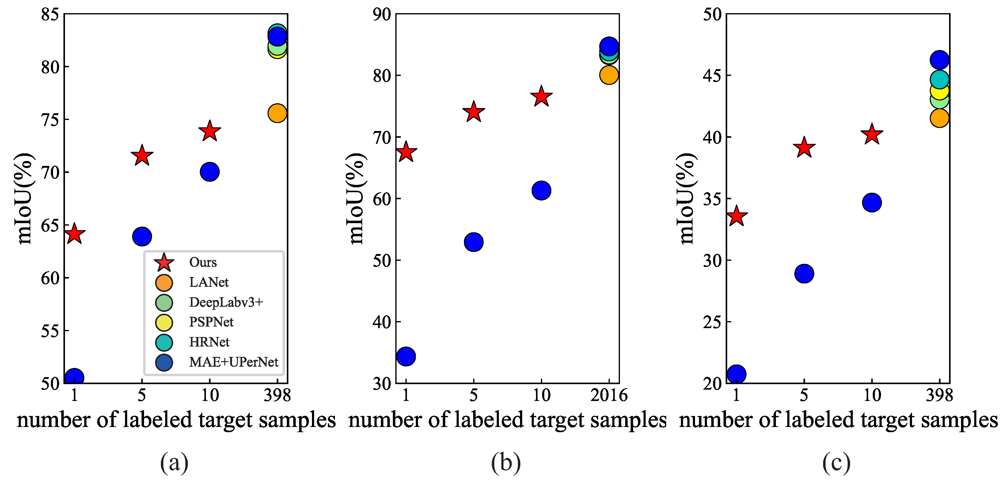
Figure 7 compares the segmentation results of the proposed method and those of the supervised counterparts with different labeled target samples. With the increase in available labeled samples, the mIoU of the proposed method gradually increased and approached the results of its supervised counterparts using all labeled target samples. This again demonstrates that the proposed method can effectively improve the segmentation results for the target RSIs using a few labeled samples, and its performance tended to be close to that of its supervised counterparts. In addition, when only a few labeled samples (e.g., 1, 5, or 10) were used for training, the mIoU of the proposed method was significantly higher than that of MAE+UPerNet, indicating its better sample efficiency.

4.4. Qualitative Results and Comparison

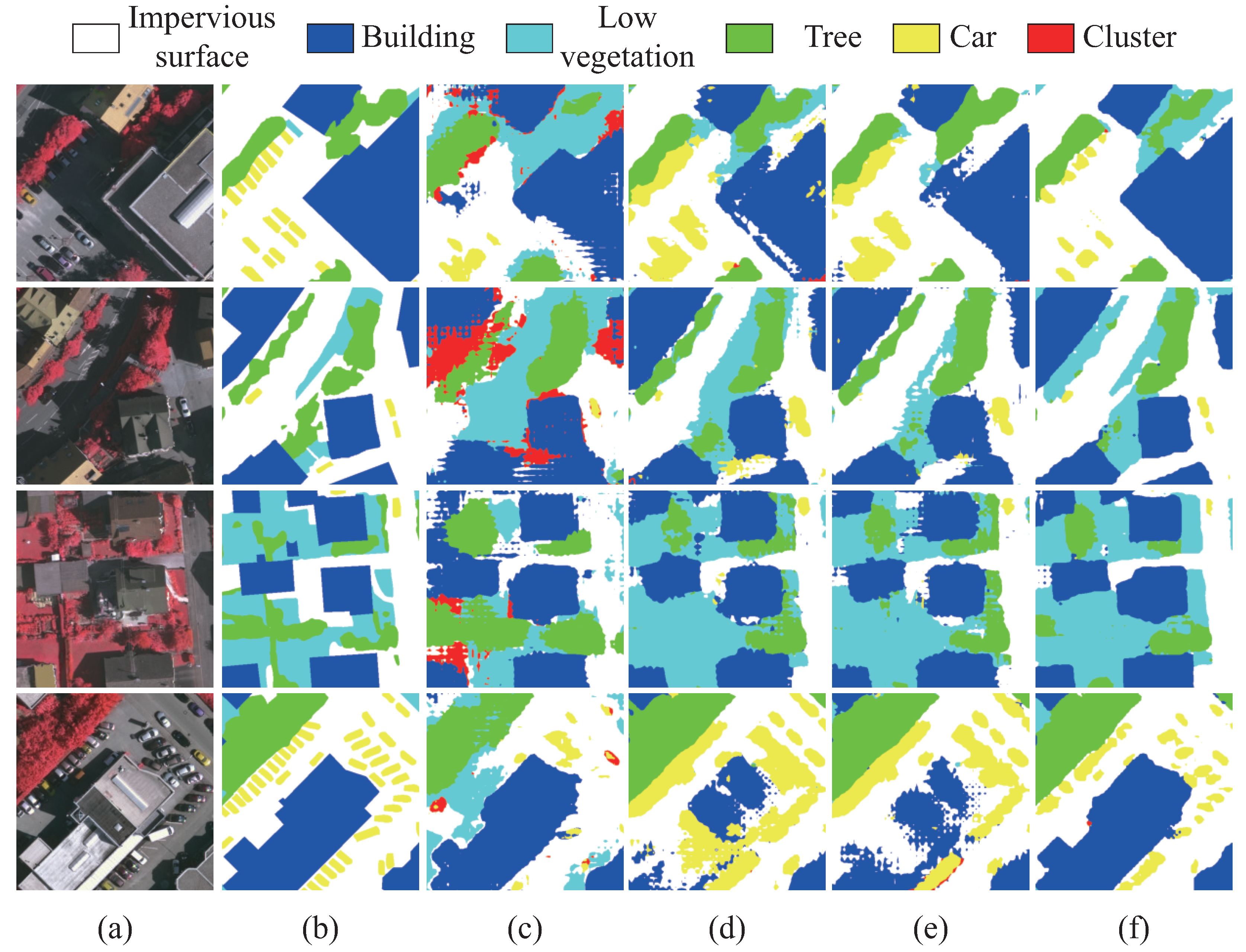
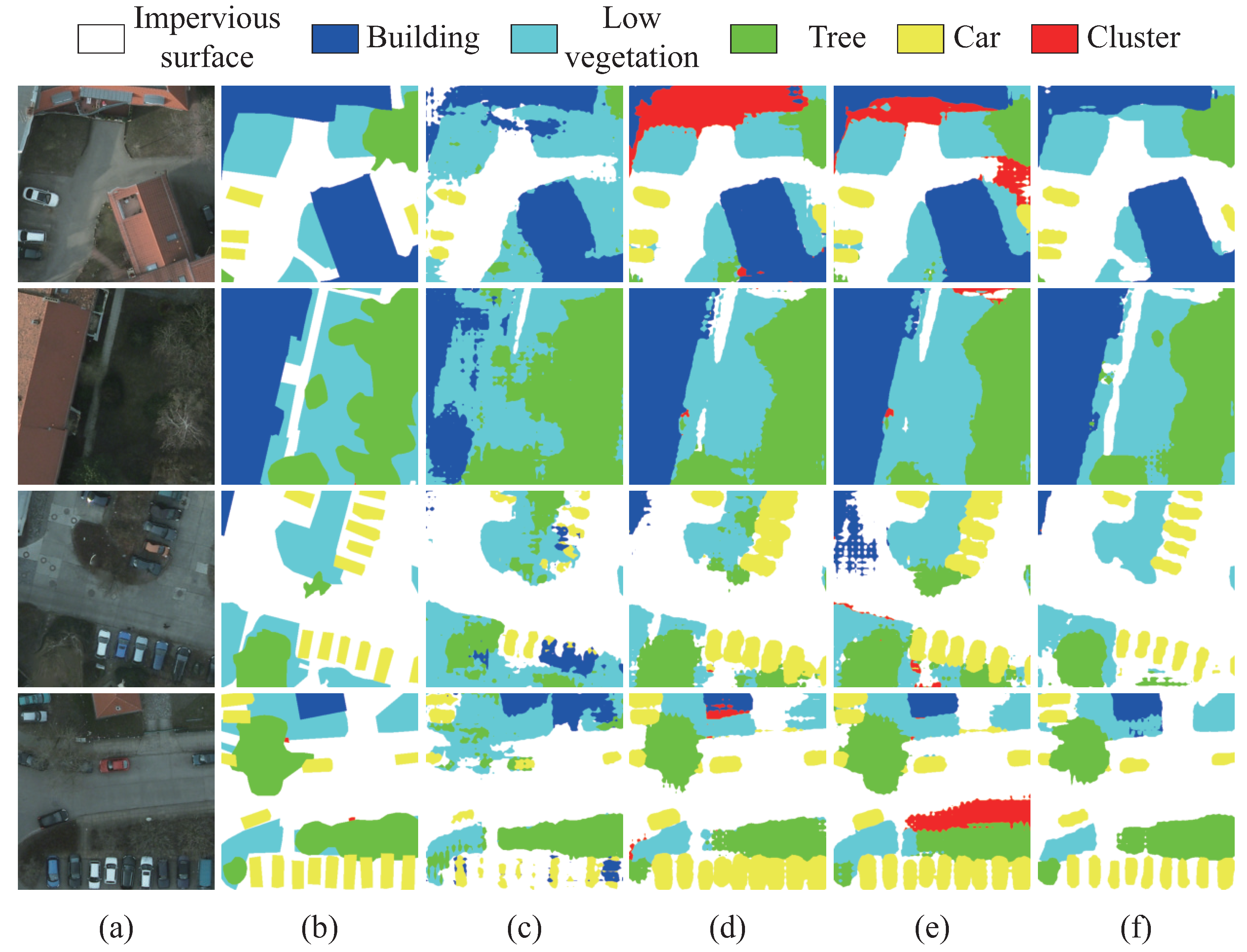
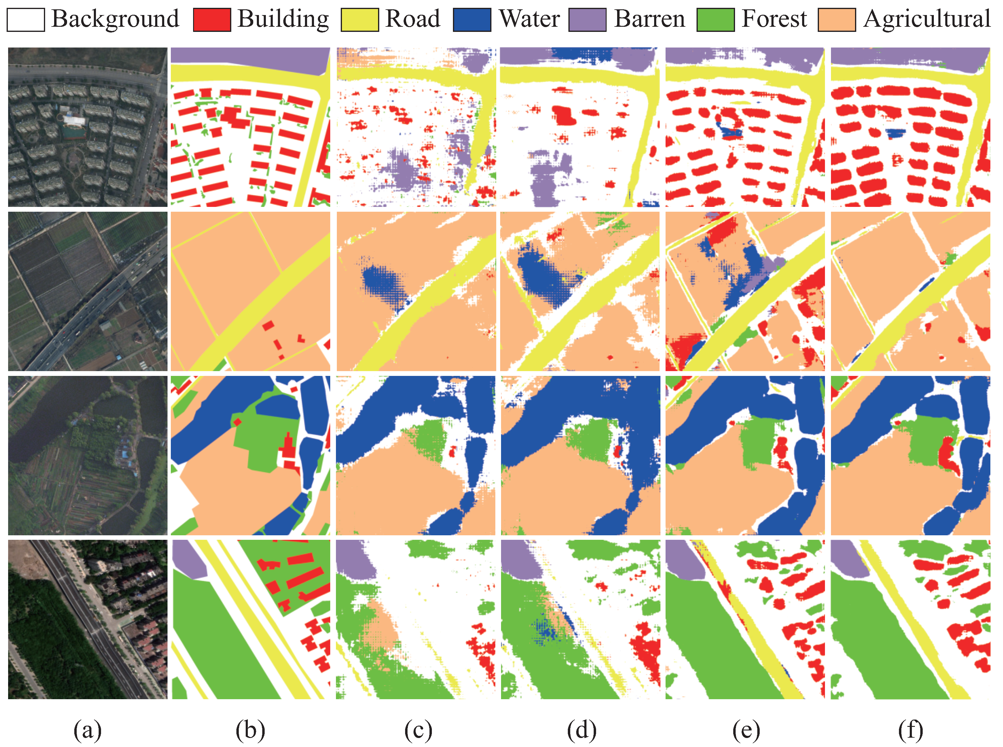
Several representative segmentation examples are visually displayed in Figure 8, Figure 9 and Figure 10 for qualitative analysis. The UDA method Zheng’s and SSDA methods Alonso’s and Hoyer’s were used for comparison with the proposed method, due to their better performance than the other methods for the corresponding types. As we can see, the segmentation maps of Zheng’s are ambiguous and scattered, and there is a lot of misrecognition and class confusion. Such segmentation maps are obviously not usable in practice. The two SSDA methods effectively improved the accuracy of the segmentation maps by utilizing some annotation information of the target RSIs. Compared with the results of Zheng’s method, the segmentation maps possess relatively complete spatial structure information, and the number of misclassified pixels was effectively reduced. However, they still suffer from unclear object boundaries and fragmented segments, which is unsatisfactory. For example, in Figure 9d,e, the smoothness of the boundaries of objects is poor, and there is a lot of noise around them. In the last row of Figure 8d,e, the complete building object is segmented into multiple ambiguous and discontinuous pieces. Compared with the above methods, the proposed method could produce more accurate segmentation maps. Benefiting from the advantages of cross-domain multi-prototypes and contradictory structure learning, there are three obvious improvements in the segmentation maps of the proposed method. First, the spatial structure is more complete, and the boundaries between adjacent objects are smoother and clearer. Second, the segmentation accuracy for small objects is significantly improved, and the discernability between them is greatly enhanced, such as the cars in the fourth row of Figure 9f and the last row of Figure 8f, and the buildings in the first row of Figure 10f. Third, the segmentation performance between classes with high similarity is improved, effectively reducing the recognition errors between these classes. For example, in the second row of Figure 9f, the proposed method could accurately recognize the complete road object, which was almost completely misclassified as low vegetation by the other methods.

5. Analysis and Discussion

5.1. Visual Analysis

In this section, a visual analysis is conducted to confirm the role of the cross-domain multi-prototypes and contradictory structure learning. First, the multi-prototypes after t-SNE [58] dimension reduction are visually displayed, as shown in Figure 11. When the number of prototypes per class was five, the prototypes belonging to different classes formed different clusters, and there was also a certain distance between multiple prototypes of the same class, suggesting that inter- and intra-class relations had been established. As the number of prototypes was increased to 5 and 10, the distance between the different clusters further widened, and the relations between the different prototypes within the same clusters were still clear, while the clusters became more compact. In particular, the sixth class cluster was a collection of many different instances without an explicit class, so the discrepancies in this class were relatively larger. As the number of prototypes was increased from 5 to 20, the prototypes of this class gradually changed from scattered to clustered, because too few prototypes were insufficient to represent the large intra-class variations.This directly demonstrated the effectiveness of the cross-domain multi-prototypes in modeling the inter- and intra-class relations.
Furthermore, to analyze the relationships between pixels and prototypes, the building class in the PD→VH task is taken as an example and the visualization results are shown in Figure 12. Specifically, in the segmentation results of the proposed method, the prototype of each pixel was obtained through the nearest prototype retrieval strategy. Then, the masks with different colors were assigned to different prototypes. At last, the input RSIs were overlaid with these masks, and the obtained results were displayed visually. It can be seen that, even within the same class of the same RSI domain, the instances with large differences had different prototypes. For example, there are four prototypes contained in the six samples in Figure 12a. In addition, in different RSI domains, the instances with similar characteristics corresponded to the same prototype, such as column 6 in Figure 12a and column 1 in Figure 12b. Undoubtedly, these observations can visually verify the representation abilities of the cross-domain multi-prototypes.
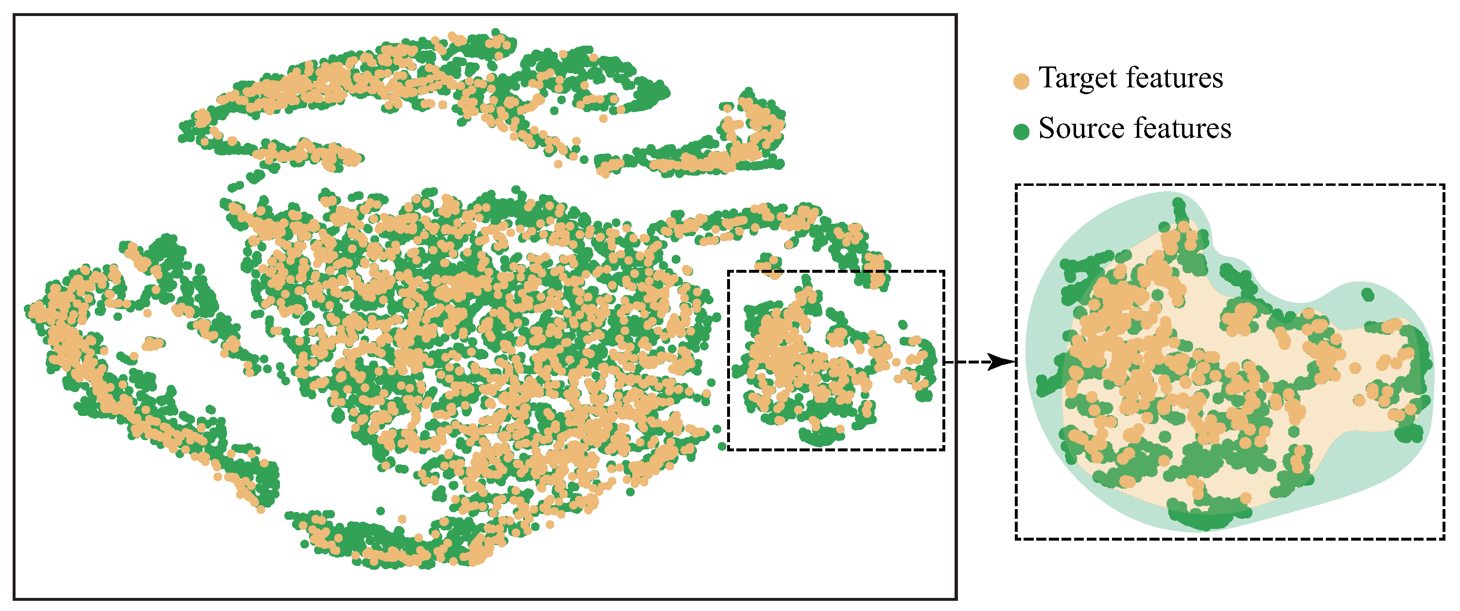
Moreover, the distributions of the source and target features after t-SNE dimension reduction were visualized, as shown in Figure 13. As we can see, the contradictory structure learning scattered the source features and clustering target features simultaneously, and the target features are generally inside the dilated boundary of the source features. At the same time, a cluster is zoomed in on, to show the details of feature distribution. In a nut shell, the better domain alignment with an enveloping form could further improve the performance of the SSDA segmentation of RSIs.

5.2. Ablation Studies

As described in Section 3.2, the proposed method combines the different advantages of cross-domain multi-prototypes, contradictory structure learning and self-supervised learning, thus effectively improving the performance in SSDA segmentation of RSIs. To verify the effectiveness of the three mechanisms for performance improvement, ablation studies were conducted and the results are listed in Table 6. With the multi-prototype constraint discarded, the proposed method only achieved 69.14%, 69.46%, and 36.37% mIoU in the three tasks, which are 2.4%, 4.55%, and 2.75% lower than the corresponding optimal values, respectively. This fully verifies its important role in improving the segmentation accuracy for target RSIs. The contradictory structure learning brought a 2.10–2.76% improvement in the mIoU, indicating its effectiveness for further improving the segmentation results. Self-supervised learning can provide high-quality pseudo-labels of target RSIs for domain adaptation training. Therefore, it also had a positive impact and further improved the mIoU by 1.47–1.91%.
In fact, the different advantages of the three approaches can complement each other and jointly improve the performance in SSDA segmentation of RSIs. Specifically, semi-supervised learning can effectively increase the number of target samples involved in prototype calculation and updating, so that the multiple sets of cross-domain prototypes can better represent the complex relations between classes in different RSI domains. In turn, the optimization of multi-prototypes can further improve the quality of pseudo-labels and thus promote the transfer and adaptation of the learned knowledge to the target domains. Meanwhile, contradictory structure learning can achieve a better feature alignment with an enveloping form and further improve the segmentation performance for the target RSIs.

5.3. Hyperparameter Analysis

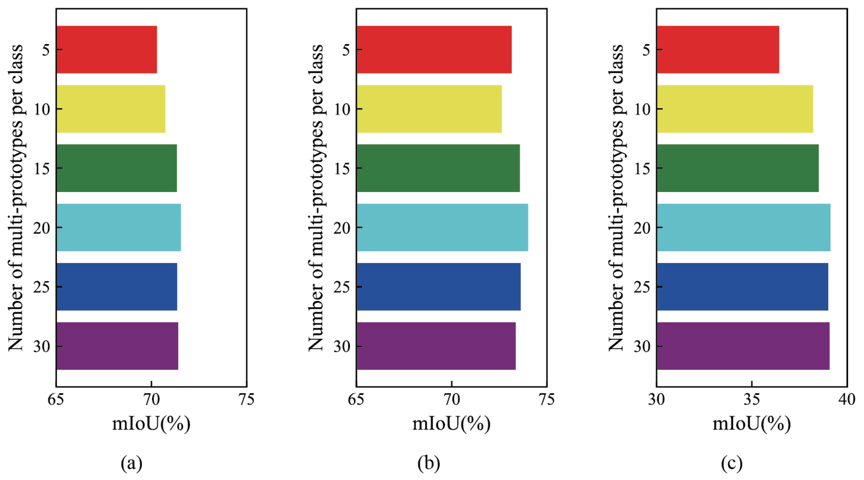
In this section, several important hyperparameters are discussed and analyzed. First of all, the relationships between the number of prototypes per class and the obtained mIoU were explored, and the results are shown in Figure 14. As we can see, the segmentation performance was limited when the number of prototypes per class was set to 5 or 10, which can be attributed to the fact that a small number of prototypes cannot adequately represent the complex inter-class discrepancies and intra-class variances. As the number of prototypes was increased, the segmentation performance showed a clear boost, while further increasing the number of prototypes beyond 20 yielded marginal returns or even a slight decrease in the mIoU. Therefore, in the proposed method, it is appropriate to set the number of prototypes per class to 20, based on the comprehensive consideration of segmentation performance and computational complexity.
Next, the relationships between the dimension of multi-prototypes and segmentation performance are analyzed, as shown in Figure 15. In short, all the curves present a trend of gradual increase at first and then a slow decline. For the different tasks, the optimal mIoU occurred when the dimensions were 1024 and 512. The reason for this can be summarized briefly as follows: With the PD dataset or the urban dataset as the target RSI, the proposed method aimed to fully adapt to the different classes and instances from a larger number of unlabeled target samples, so a larger number of dimensions was necessary to learn more complex and rich information. However, with the VH dataset as the target RSIs, the number of unlabeled target samples participating in domain adaptation training was only 398, which was a smaller value than those for the other two tasks, so the optimal value of the dimensions was relatively small in the PD→VH task. Actually, the different optimal values for the dimensions in different tasks indirectly confirmed the advantages of multi-prototypes for capturing intra-class and inter-class relations.
Last but not least, the influence of the hyperparameter β on the segmentation performance of the proposed method was explored. As expressed in Equation (12), a larger value of β increased the component of the contradictory structure learning in the process of domain adaptation training, while a smaller value of β would undoubtedly weaken its role in improving the domain alignment. According to the statistical results in Table 7, when the value of β was too large or too small, the mIoU declined to varying degrees, and the value of β corresponding to the optimal segmentation performance was 0.1.

6. Conclusions

In this paper, a novel SSDA method for RSI domain adaptation segmentation was proposed, effectively improving the segmentation results for target RSIs with a few labeled target samples. Specifically, the proposed method consisted of three different learning mechanisms: cross-domain multi-prototype constraint, contradictory structure learning, and self-supervised learning. On the one hand, considering the inter-domain discrepancies and intra-domain variations in different RSIs, building a set of prototypes for each class could better model the complex inter- and intra-class relations. On the other hand, the multiple sets of prototypes were calculated and updated jointly by both the source and target samples, effectively promoting the utilization and integration of the feature information in different domains. Meanwhile, through gathering target features and scattering source features simultaneously, the designed contradictory structure learning mechanism can effectively improve domain alignment through an enveloping form. In addition, self-supervised learning can effectively increase the number of target samples involved in multi-prototype updating and domain adaptation training, further improving the generalization and adaptation to target RSI domains. The experimental results demonstrated that the proposed method can, not only effectively improve the performance of SSDA segmentation of RSIs, but also significantly narrow the gap with its supervised counterparts, with only a few labeled target samples available. This paper also opens a new avenue for future work on RSI domain adaptation segmentation.
It should be noted that the cross-domain multi-prototypes and contradictory structure learning modules designed in this paper could also be embedded into existing domain adaptation frameworks, such as adversarial learning methods and so on. However, the effects of this remain to be further explored. In addition, the experimental settings were limited to spaceborne RSI datasets and airborne RSI datasets, and the domain adaptation method between spaceborne and airborne RSIs is under-explored. Finally, the multi-stage domain adaptation process from a single source RSI to multiple target RSIs also needs further study. The above works could be further developed and implemented on the basis of this paper.

Author Contributions

Methodology, K.G. and A.Y.; investigation, A.Y., X.Y. and C.Q.; resources, A.Y. and X.Y.; writing—original draft preparation, K.G.; writing—review and editing, A.Y.; visualization, K.G., B.L. and F.Z.; supervision, A.Y. and X.Y. All authors have read and agreed to the published version of the manuscript.

Funding

This research was funded by National Natural Science Foundation of China under grants 42130112, 42101458, and 41801388.

Data Availability Statement

Publicly available datasets were analyzed in this study, which can be found here: https://www.isprs.org/education/benchmarks/UrbanSemLab (accessed on 8 May 2023).

Acknowledgments

The authors would like to thank all the professionals for kindly providing the codes associated with the experiments.

Conflicts of Interest

The authors declare no conflict of interest.

References

  1. Long, J.; Shelhamer, E.; Darrell, T. Fully convolutional networks for semantic segmentation. In Proceedings of the 2015 IEEE Conference on Computer Vision and Pattern Recognition (CVPR), Boston, MA, USA, 7–12 June 2015; pp. 3431–3440. [Google Scholar] [CrossRef] [Green Version]
  2. Zhao, H.S.; Shi, J.P.; Qi, X.J.; Wang, X.G.; Jia, J.Y. Pyramid Scene Parsing Network. arXiv 2017, arXiv:1612.01105. [Google Scholar] [CrossRef] [Green Version]
  3. Xiao, T.T.; Liu, Y.C.; Zhou, B.L.; Jiang, Y.N.; Sun, J. Unified Perceptual Parsing for Scene Understanding. arXiv 2018, arXiv:1807.10221. [Google Scholar] [CrossRef] [Green Version]
  4. Ma, L.; Liu, Y.; Zhang, X.; Ye, Y.; Yin, G.; Johnson, B.A. Deep learning in remote sensing applications: A meta-analysis and review. ISPRS J. Photogramm. Remote Sens. 2019, 152, 166–177. [Google Scholar] [CrossRef]
  5. Gao, K.; Liu, B.; Yu, X.; Yu, A. Unsupervised Meta Learning With Multiview Constraints for Hyperspectral Image Small Sample set Classification. IEEE Trans. Image Process. 2022, 31, 3449–3462. [Google Scholar] [CrossRef] [PubMed]
  6. Kotaridis, I.; Lazaridou, M. Remote sensing image segmentation advances: A meta-analysis. ISPRS J. Photogramm. Remote Sens. 2021, 173, 309–322. [Google Scholar] [CrossRef]
  7. Zhang, L.; Zhang, L. Artificial Intelligence for Remote Sensing Data Analysis: A review of challenges and opportunities. IEEE Geosci. Remote Sens. Mag. 2022, 10, 270–294. [Google Scholar] [CrossRef]
  8. Luo, M.; Ji, S. Cross-spatiotemporal land-cover classification from VHR remote sensing images with deep learning based domain adaptation. ISPRS J. Photogramm. Remote Sens. 2022, 191, 105–128. [Google Scholar] [CrossRef]
  9. Zhao, S.; Yue, X.; Zhang, S.; Li, B.; Zhao, H.; Wu, B.; Krishna, R.; Gonzalez, J.E.; Sangiovanni-Vincentelli, A.L.; Seshia, S.A.; et al. A Review of Single-Source Deep Unsupervised Visual Domain Adaptation. IEEE Trans. Neural Netw. Learn. Syst. 2022, 33, 473–493. [Google Scholar] [CrossRef]
  10. Sun, X.; Wang, P.; Lu, W.; Zhu, Z.; Lu, X.; He, Q.; Li, J.; Rong, X.; Yang, Z.; Chang, H.; et al. RingMo: A Remote Sensing Foundation Model with Masked Image Modeling. IEEE Trans. Geosci. Remote Sens. 2022, 1. [Google Scholar] [CrossRef]
  11. Xu, Q.; Yuan, X.; Ouyang, C. Class-Aware Domain Adaptation for Semantic Segmentation of Remote Sensing Images. IEEE Trans. Geosci. Remote Sens. 2022, 60, 1–17. [Google Scholar] [CrossRef]
  12. Wang, J.; Zheng, Z.; Ma, A.; Lu, X.; Zhong, Y. LoveDA: A Remote Sensing Land-Cover Dataset for Domain Adaptive Semantic Segmentation. CoRR 2021, abs/2110.08733. Available online: http://xxx.lanl.gov/abs/2110.08733 (accessed on 1 July 2020.).
  13. Zheng, A.; Wang, M.; Li, C.; Tang, J.; Luo, B. Entropy Guided Adversarial Domain Adaptation for Aerial Image Semantic Segmentation. IEEE Trans. Geosci. Remote Sens. 2022, 60, 1–14. [Google Scholar] [CrossRef]
  14. Saito, K.; Kim, D.; Sclaroff, S.; Darrell, T.; Saenko, K. Semi-supervised Domain Adaptation via Minimax Entropy. arXiv 2019, arXiv:1904.06487. [Google Scholar] [CrossRef] [Green Version]
  15. Li, K.; Liu, C.; Zhao, H.D.; Zhang, Y.L.; Fu, Y.; IEEE. ECACL: A Holistic Framework for Semi-Supervised Domain Adaptation. In Proceedings of the IEEE/CVF International Conference on Computer Vision, Montreal, QC, Canada, 10–17 October 2021. [Google Scholar] [CrossRef]
  16. Yan, Z.; Wu, Y.; Li, G.; Qin, Y.; Han, X.; Cui, S. Multi-level Consistency Learning for Semi-supervised Domain Adaptation. In Proceedings of the IJCAI, Vienna, Austria, 25 July 2022; pp. 1530–1536. [Google Scholar]
  17. Wang, Z.H.; Wei, Y.C.; Feris, R.; Xiong, J.J.; Hwu, W.M.; Huang, T.S.; Shi, H.H.; SOC, I.C. Alleviating Semantic-level Shift: A Semi-supervised Domain Adaptation Method for Semantic Segmentation. arXiv 2020, arXiv:2004.00794. [Google Scholar] [CrossRef]
  18. Alonso, I.; Sabater, A.; Ferstl, D.; Montesano, L.; Murillo, A.C.; IEEE. Semi-Supervised Semantic Segmentation with Pixel-Level Contrastive Learning from a Class-wise Memory Bank. arXiv 2021, arXiv:2104.13415. [Google Scholar] [CrossRef]
  19. Berthelot, D.; Roelofs, R.; Sohn, K.; Carlini, N.; Kurakin, A. AdaMatch: A Unified Approach to Semi-Supervised Learning and Domain Adaptation. In Proceedings of the International Conference on Learning Representations, Virtual Event, 25–29 April 2022. [Google Scholar]
  20. Jiang, X.; Zhou, N.; Li, X. Few-Shot Segmentation of Remote Sensing Images Using Deep Metric Learning. IEEE Geosci. Remote Sens. Lett. 2022, 19, 1–5. [Google Scholar] [CrossRef]
  21. Osco, L.P.; Marcato Junior, J.; Marques Ramos, A.P.; de Castro Jorge, L.A.; Fatholahi, S.N.; de Andrade Silva, J.; Matsubara, E.T.; Pistori, H.; Gonçalves, W.N.; Li, J. A review on deep learning in UAV remote sensing. Int. J. Appl. Earth Obs. Geoinf. 2021, 102, 102456. [Google Scholar] [CrossRef]
  22. Gao, K.; Liu, B.; Yu, X.; Qin, J.; Zhang, P.; Tan, X. Deep Relation Network for Hyperspectral Image Few-Shot Classification. Remote Sens. 2020, 12, 923. [Google Scholar] [CrossRef] [Green Version]
  23. Ronneberger, O.; Fischer, P.; Brox, T. U-Net: Convolutional Networks for Biomedical Image Segmentation. arXiv 2015, arXiv:1505.04597. [Google Scholar] [CrossRef] [Green Version]
  24. Diakogiannis, F.I.; Waldner, F.; Caccetta, P.; Wu, C. ResUNet-a: A deep learning framework for semantic segmentation of remotely sensed data. ISPRS J. Photogramm. Remote Sens. 2020, 162, 94–114. [Google Scholar] [CrossRef] [Green Version]
  25. Liu, Y.; Fan, B.; Wang, L.; Bai, J.; Xiang, S.; Pan, C. Semantic labeling in very high resolution images via a self-cascaded convolutional neural network. ISPRS J. Photogramm. Remote Sens. 2018, 145, 78–95. [Google Scholar] [CrossRef] [Green Version]
  26. Ding, L.; Tang, H.; Bruzzone, L. LANet: Local Attention Embedding to Improve the Semantic Segmentation of Remote Sensing Images. IEEE Trans. Geosci. Remote Sens. 2021, 59, 426–435. [Google Scholar] [CrossRef]
  27. Li, R.; Zheng, S.; Zhang, C.; Duan, C.; Su, J.; Wang, L.; Atkinson, P.M. Multiattention Network for Semantic Segmentation of Fine-Resolution Remote Sensing Images. IEEE Trans. Geosci. Remote Sens. 2022, 60, 1–13. [Google Scholar] [CrossRef]
  28. He, Q.; Sun, X.; Diao, W.; Yan, Z.; Yin, D.; Fu, K. Transformer-induced graph reasoning for multimodal semantic segmentation in remote sensing. ISPRS J. Photogramm. Remote Sens. 2022, 193, 90–103. [Google Scholar] [CrossRef]
  29. He, X.; Zhou, Y.; Zhao, J.; Zhang, D.; Yao, R.; Xue, Y. Swin Transformer Embedding UNet for Remote Sensing Image Semantic Segmentation. IEEE Trans. Geosci. Remote Sens. 2022, 60, 1–15. [Google Scholar] [CrossRef]
  30. Wang, L.; Li, R.; Zhang, C.; Fang, S.; Duan, C.; Meng, X.; Atkinson, P.M. UNetFormer: A UNet-like transformer for efficient semantic segmentation of remote sensing urban scene imagery. ISPRS J. Photogramm. Remote Sens. 2022, 190, 196–214. [Google Scholar] [CrossRef]
  31. Chen, Z.; Shang, Y.; Python, A.; Cai, Y.; Yin, J. DB-BlendMask: Decomposed Attention and Balanced BlendMask for Instance Segmentation of High-Resolution Remote Sensing Images. IEEE Trans. Geosci. Remote Sens. 2022, 60, 1–15. [Google Scholar] [CrossRef]
  32. Zhang, T.; Zhang, X.; Zhu, P.; Tang, X.; Li, C.; Jiao, L.; Zhou, H. Semantic Attention and Scale Complementary Network for Instance Segmentation in Remote Sensing Images. IEEE Trans. Cybern. 2022, 52, 10999–11013. [Google Scholar] [CrossRef]
  33. Ma, A.; Wang, J.; Zhong, Y.; Zheng, Z. FactSeg: Foreground Activation-Driven Small Object Semantic Segmentation in Large-Scale Remote Sensing Imagery. IEEE Trans. Geosci. Remote Sens. 2022, 60, 1–16. [Google Scholar] [CrossRef]
  34. Chen, X.; Pan, S.; Chong, Y. Unsupervised Domain Adaptation for Remote Sensing Image Semantic Segmentation Using Region and Category Adaptive Domain Discriminator. IEEE Trans. Geosci. Remote Sens. 2022, 60, 1–13. [Google Scholar] [CrossRef]
  35. Chen, J.; Zhu, J.; Guo, Y.; Sun, G.; Zhang, Y.; Deng, M. Unsupervised Domain Adaptation for Semantic Segmentation of High-Resolution Remote Sensing Imagery Driven by Category-Certainty Attention. IEEE Trans. Geosci. Remote Sens. 2022, 60, 1–15. [Google Scholar] [CrossRef]
  36. Chen, H.; Zhang, H.; Yang, G.; Li, S.; Zhang, L. A Mutual Information Domain Adaptation Network for Remotely Sensed Semantic Segmentation. IEEE Trans. Geosci. Remote Sens. 2022, 60, 1–16. [Google Scholar] [CrossRef]
  37. Gui, J.; Sun, Z.; Wen, Y.; Tao, D.; Ye, J. A Review on Generative Adversarial Networks: Algorithms, Theory, and Applications. IEEE Trans. Knowl. Data Eng. 2021, 35, 3313–3332. [Google Scholar] [CrossRef]
  38. Bai, L.; Du, S.; Zhang, X.; Wang, H.; Liu, B.; Ouyang, S. Domain Adaptation for Remote Sensing Image Semantic Segmentation: An Integrated Approach of Contrastive Learning and Adversarial Learning. IEEE Trans. Geosci. Remote Sens. 2022, 60, 1–13. [Google Scholar] [CrossRef]
  39. Wang, J.; Ma, A.; Zhong, Y.; Zheng, Z.; Zhang, L. Cross-sensor domain adaptation for high spatial resolution urban land-cover mapping: From airborne to spaceborne imagery. Remote Sens. Environ. 2022, 277, 113058. [Google Scholar] [CrossRef]
  40. Yan, L.; Fan, B.; Xiang, S.; Pan, C. CMT: Cross Mean Teacher Unsupervised Domain Adaptation for VHR Image Semantic Segmentation. IEEE Geosci. Remote Sens. Lett. 2022, 19, 1–5. [Google Scholar] [CrossRef]
  41. Li, Y.; Shi, T.; Zhang, Y.; Chen, W.; Wang, Z.; Li, H. Learning deep semantic segmentation network under multiple weakly-supervised constraints for cross-domain remote sensing image semantic segmentation. ISPRS J. Photogramm. Remote Sens. 2021, 175, 20–33. [Google Scholar] [CrossRef]
  42. Zhao, Y.; Gao, H.; Guo, P.; Sun, Z. ResiDualGAN: Resize-Residual DualGAN for Cross-Domain Remote Sensing Images Semantic Segmentation. CoRR 2022, abs/2201.11523. Available online: http://xxx.lanl.gov/abs/2201.11523 (accessed on 1 July 2020.).
  43. Tasar, O.; Happy, S.L.; Tarabalka, Y.; Alliez, P. ColorMapGAN: Unsupervised Domain Adaptation for Semantic Segmentation Using Color Mapping Generative Adversarial Networks. IEEE Trans. Geosci. Remote Sens. 2020, 58, 7178–7193. [Google Scholar] [CrossRef] [Green Version]
  44. Chen, S.; Jia, X.; He, J.; Shi, Y.; Liu, J. Semi-supervised Domain Adaptation based on Dual-level Domain Mixing for Semantic Segmentation. CoRR 2021, abs/2103.04705. [Google Scholar]
  45. Zhou, T.; Wang, W.; Konukoglu, E.; Van Goo, L. Rethinking Semantic Segmentation: A Prototype View. In Proceedings of the 2022 IEEE/CVF Conference on Computer Vision and Pattern Recognition (CVPR), New Orleans, LA, USA, 18–24 June 2022; pp. 2572–2583. [Google Scholar] [CrossRef]
  46. Cuturi, M. Sinkhorn Distances: Lightspeed Computation of Optimal Transport. In Proceedings of the Advances in Neural Information Processing Systems; Burges, C., Bottou, L., Welling, M., Ghahramani, Z., Weinberger, K., Eds.; Curran Associates, Inc.: Red Hook, NY, USA, 2013; Volume 26. [Google Scholar]
  47. Zhang, X.; Zhao, R.; Qiao, Y.; Li, H. RBF-Softmax: Learning Deep Representative Prototypes with Radial Basis Function Softmax. In Proceedings of the Computer Vision—ECCV 2020, Glasgow, UK, 23—28 August 2020; Vedaldi, A., Bischof, H., Brox, T., Frahm, J.M., Eds.; Springer International Publishing: Cham, Switzerkand, 2020; pp. 296–311. [Google Scholar]
  48. Qin, C.; Wang, L.; Ma, Q.; Yin, Y.; Wang, H.; Fu, Y. Semi-supervised Domain Adaptive Structure Learning. CoRR 2021, abs/2112.06161. Available online: http://xxx.lanl.gov/abs/2112.06161 (accessed on 1 July 2020.).
  49. Pan, X.; Ge, C.; Lu, R.; Song, S.; Chen, G.; Huang, Z.; Huang, G. On the Integration of Self-Attention and Convolution. In Proceedings of the 2022 IEEE/CVF Conference on Computer Vision and Pattern Recognition (CVPR), New Orleans, LA, USA, 19–20 June 2022; pp. 805–815. [Google Scholar] [CrossRef]
  50. Fang, B.; Kou, R.; Pan, L.; Chen, P. Category-Sensitive Domain Adaptation for Land Cover Mapping in Aerial Scenes. Remote Sens. 2019, 11, 2631. [Google Scholar] [CrossRef] [Green Version]
  51. Loshchilov, I.; Hutter, F. Decoupled Weight Decay Regularization. In Proceedings of the 7th International Conference on Learning Representations, ICLR 2019, New Orleans, LA, USA, 6–9 May 2019. [Google Scholar]
  52. Tranheden, W.; Olsson, V.; Pinto, J.; Svensson, L. DACS: Domain Adaptation via Cross-domain Mixed Sampling. In Proceedings of the 2021 IEEE Winter Conference on Applications of Computer Vision (WACV), Waikoloa, HI, USA, 5–9 January 2021; pp. 1378–1388. [Google Scholar] [CrossRef]
  53. Zheng, Z.D.; Yang, Y. Unsupervised Scene Adaptation with Memory Regularization in vivo. arXiv 2020, arXiv:1912.11164. [Google Scholar]
  54. Vu, T.H.; Jain, H.; Bucher, M.; Cord, M.; Pérez, P. ADVENT: Adversarial Entropy Minimization for Domain Adaptation in Semantic Segmentation. In Proceedings of the 2019 IEEE/CVF Conference on Computer Vision and Pattern Recognition (CVPR), Long Beach, CA, USA, 15–20 June 2019; pp. 2512–2521. [Google Scholar] [CrossRef] [Green Version]
  55. Zhao, Y.; Guo, P.; Gao, H.; Chen, X. Depth-Assisted ResiDualGAN for Cross-Domain Aerial Images Semantic Segmentation. CoRR 2022, abs/2208.09823. Available online: http://xxx.lanl.gov/abs/2208.09823 (accessed on 1 July 2020.). [CrossRef]
  56. Chen, L.C.E.; Zhu, Y.K.; Papandreou, G.; Schroff, F.; Adam, H. Encoder-Decoder with Atrous Separable Convolution for Semantic Image Segmentation. arXiv 2018, arXiv:1802.02611. [Google Scholar] [CrossRef] [Green Version]
  57. Wang, J.; Sun, K.; Cheng, T.; Jiang, B.; Deng, C.; Zhao, Y.; Liu, D.; Mu, Y.; Tan, M.; Wang, X.; et al. Deep High-Resolution Representation Learning for Visual Recognition. IEEE Trans. Pattern Anal. Mach. Intell. 2021, 43, 3349–3364. [Google Scholar] [CrossRef] [PubMed] [Green Version]
  58. van der Maaten, L.; Hinton, G.E. Visualizing Data using t-SNE. J. Mach. Learn. Res. 2008, 9, 2579–2605. [Google Scholar]
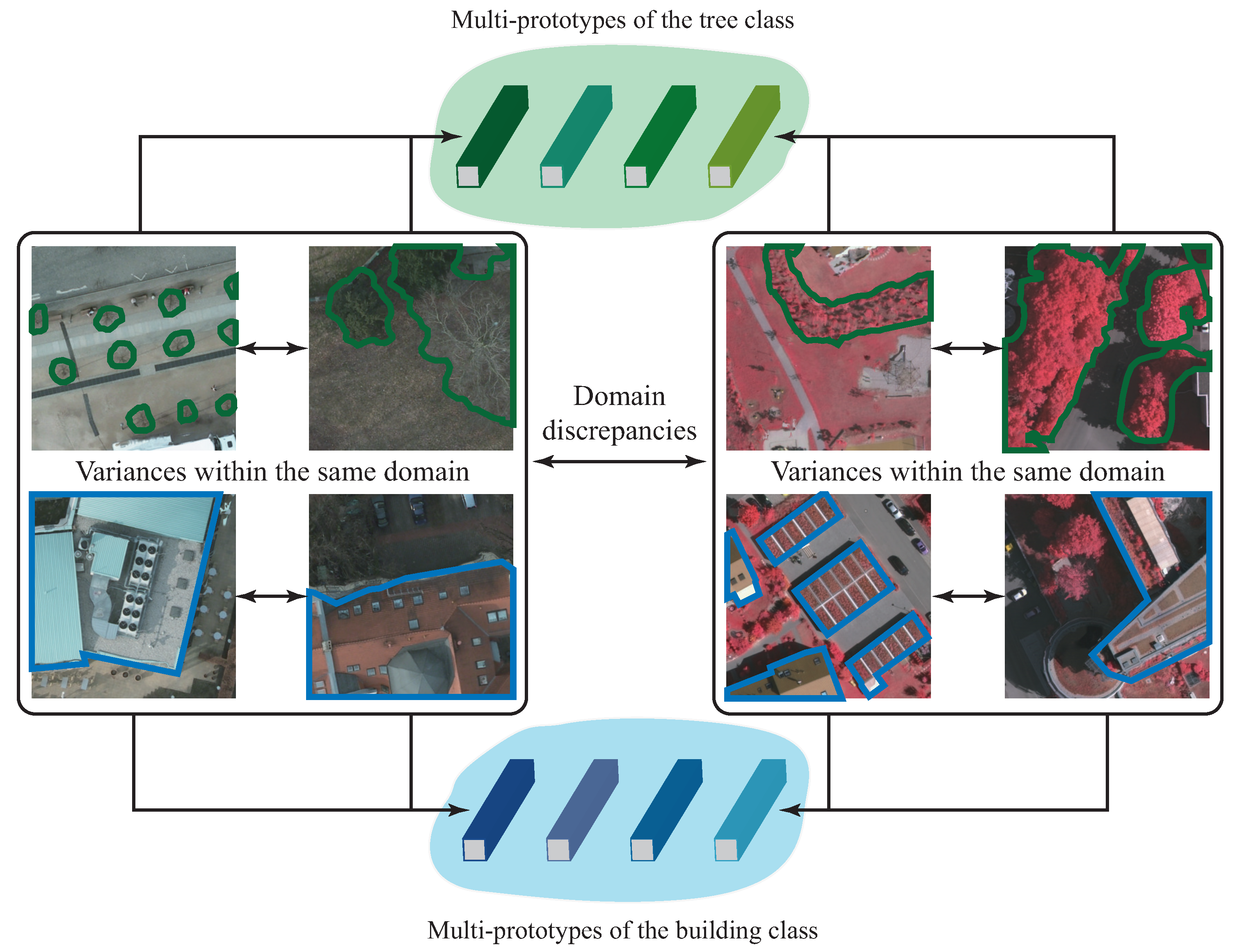
Figure 1. Schematic of inter-domain discrepancies and intra-domain variations. Given that there are such diverse and disparate instances within a class, each class is represented as a set of prototypes, which are calculated and updated jointly by the samples from source and target domains.
Remotesensing 15 03398 g001
Figure 2. Schematic of contradictory structure learning. Different colors represent different classes. Through target gathering and source scattering simultaneously, the target features are within the dilated boundary of the source features, thus achieving better domain alignment with an enveloping form.
Remotesensing 15 03398 g002
Figure 3. Workflow of the proposed method. The green line, orange line, and red line represent the data flows of labeled source samples, unlabeled target samples, and labeled target samples. The dashed line represents a smaller percentage of the gradient along that branch during loss backpropagation. The symbols L c e , L p p c , and L p p d denote the supervised loss, pixel-prototype contrastive loss, and pixel-prototype distance loss. The symbols L h t and L h s are the losses for target gathering and source scattering, respectively, and the symbol L h t is the self-supervised loss.
Remotesensing 15 03398 g003
Figure 4. Optimizing the learning process of cross-domain multi-prototypes from three different levels. (a) Inter-class relation. (b) Inter-cluster relation. (c) Intra-cluster compactness.
Remotesensing 15 03398 g004
Figure 5. Flowchart of the ACmix structure.
Remotesensing 15 03398 g005
Figure 6. Comparison of the SSDA methods and proposed method with different numbers of labeled target samples. (a) PD→VH. (b) VH→PD. (c) Rural→Urban.
Remotesensing 15 03398 g006
Figure 7. Comparison of the proposed method and supervised learning methods with different numbers of labeled target samples. (a) PD→VH. (b) VH→PD. (c) Rural→Urban.
Remotesensing 15 03398 g007
Figure 8. Segmentation maps of the different methods in the PD→VH task. (a) RSIs. (b) Ground truth. (c) Zheng’s. (d) Alonso’s. (e) Hoyer’s. (f) Ours.
Remotesensing 15 03398 g008
Figure 9. Segmentation maps of the different methods in the VH→PD task. (a) RSIs. (b) Ground truth. (c) Zheng’s. (d) Alonso’s. (e) Hoyer’s. (f) Ours.
Remotesensing 15 03398 g009
Figure 10. Segmentation maps of the different methods in the Rural→Urban task. (a) RSIs. (b) Ground truth. (c) Zheng’s. (d) Alonso’s. (e) Hoyer’s. (f) Ours.
Remotesensing 15 03398 g010
Figure 11. Visualization of the cross-domain multi-prototypes in the PD→VH task. (ac) Correspond to 5, 10, and 20 prototypes per class.
Remotesensing 15 03398 g011
Figure 12. Visualization of the relationships between pixels and prototypes with the building class as an example in the PD→VH task. The first row and the second row show the RSIs and their corresponding ground truths, respectively. The third row displays the weighted addition results of the masks of different prototypes and RSIs. The subfigures (a,b) display several representative samples in the PD and VH datasets, respectively. It can be seen that, the instances with large differences corresponded to different prototypes and similar instances corresponded to the same prototypes, verifying the representation abilities of the cross-domain multi-prototypes.
Remotesensing 15 03398 g012
Figure 13. Visualization of the distributions of source and target features.
Remotesensing 15 03398 g013
Figure 14. Relationships between the number of cross-domain multi-prototypes per class and mIoU. (a) PD→VH. (b) VH→PD. (c) Rural→Urban.
Remotesensing 15 03398 g014
Figure 15. Relationship between the dimensions of cross-domain multi-prototypes and mIoU.
Remotesensing 15 03398 g015
Table 1. Details of the different RSI datasets.
RSIsTypesCoverageResolutionBands
VHAirborne1.38 km 2 0.09 mIRRG
PDAirborne3.42 km 2 0.05 mRGB
LoveDASpaceborne536.15 km 2 0.3 mRGB
Table 2. Task settings. The symbols S, U t , and T represent the labeled source samples, unlabeled target samples, and labeled target samples for training, while U v represents the target samples for evaluation.
TasksS U t T U v
PD→VH34563985344
VH→PD344201653456
Rural→Urban136667751156
Table 3. Segmentation results of the different methods on the VH dataset. Bold values represent the results of the proposed method.
TypesSettingsMethodsPAImpervious
Surface
BuildingLow
Vegetation
TreeCarmIoU
UDAtraining:
S,
U t without labels
evaluating:
U v
DACS62.2758.0980.6316.2641.7043.4848.03
MRNet65.3154.1175.3916.1654.9929.3946.01
Advent65.5155.4368.4920.7359.0228.2846.39
Zheng’s67.5055.0672.7331.5455.4021.7347.29
RDG66.4453.8874.2222.5258.1129.8947.72
DRDG69.2355.7375.0821.3460.0233.3949.11
SSDAtraining:
S, T,
U t without labels
evaluating:
U v
DACS (SSDA)73.4559.3487.5116.1343.0446.3750.48
Zheng’s (SSDA)69.2757.2574.6423.7759.4323.7647.77
RDG (SSDA)71.3456.3376.1223.6059.1332.2449.48
MME73.4865.0666.8237.3958.3032.6952.05
CDAC76.7570.3872.5436.3663.4628.5954.27
Alonso’s80.3271.5977.4849.3370.4538.6461.50
Hoyer’s82.0474.1679.4853.3670.7743.0564.16
Ours86.4581.5989.4960.6671.8054.1871.54
SLtraining:
U t with labels
evaluating:
U v
LANet88.4182.9390.0866.2576.8161.8275.58
PSPNet90.4785.6692.2170.1680.3179.9081.65
DeepLabv3+90.6386.1592.6670.0880.3680.5581.96
HRNet91.0587.2193.2371.0980.5883.6483.15
MAE+UPerNet91.5787.6193.9272.6681.6678.2882.83
Table 4. Segmentation results of the different methods on the PD dataset. Bold values represent the results of the proposed method.
TypesSettingsMethodsPAImpervious
Surface
BuildingLow
Vegetation
TreeCarmIoU
UDAtraining:
S,
U t without labels
evaluating:
U v
DACS57.1945.7651.8839.0115.6143.6239.18
MRNet58.2548.5654.3436.4026.2054.5244.00
Advent60.0349.8054.8540.1926.9446.7143.70
Zheng’s60.8947.6348.7734.9241.1751.5844.81
RDG60.6352.1748.0040.0137.6944.4744.47
DRDG62.5454.0550.5339.1439.1547.0845.99
SSDAtraining:
S, T,
U t without labels
evaluating:
U v
DACS (SSDA)60.8348.3157.7743.0216.3847.0942.51
Zheng’s (SSDA)62.9653.6352.4842.1438.1752.2647.84
RDG (SSDA)61.9851.3548.4543.0440.4353.9147.44
MME61.0348.9251.6231.7750.5851.4146.86
CDAC64.7160.0361.4720.0144.3255.8248.33
Alonso’s78.0071.9473.9264.6159.2264.3266.80
Hoyer’s79.7171.7478.0265.9061.6168.7969.21
Ours82.1972.2381.7168.2664.8982.9874.01
SLtraining:
U t with labels
evaluating:
U v
LANet86.6880.4188.5371.2069.6390.4880.05
PSPNet89.2384.1991.6574.1874.7491.5783.27
DeepLabv3+89.3184.0292.2574.1974.9191.5683.39
HRNet89.6985.1692.8974.7675.1091.5183.88
MAE+UPerNet90.2085.9593.2576.3376.0891.8284.69
Table 5. Segmentation results of different methods on the Urban dataset. Bold values represent the results of the proposed method.
TypesSettingsMethodsPABackgroundBuildingRoadWaterBarrenForestAgriculturalmIoU
UDAtraining:
S,
U t without labels
evaluating:
U v
DACS53.8546.3337.8732.3935.6121.3321.4214.7929.96
MRNet51.0330.8342.3036.0743.1226.8925.8310.3830.77
Advent50.6629.1242.1436.4243.8527.3026.4812.5631.12
Zheng’s52.6943.7337.2332.2248.9221.2626.6510.9731.57
RDG53.8549.5836.1736.5855.7319.0715.6815.3732.60
SSDAtraining:
S, T,
U t without labels
evaluating:
U v
DACS (SSDA)54.1347.9338.0234.0337.4320.9422.0615.3930.83
Zheng’s (SSDA)53.2544.5737.9532.9650.1321.7927.0312.8332.47
RDG (SSDA)54.9249.9737.9437.0456.5620.9718.6115.0733.74
MME53.9641.1240.9833.6553.9027.0620.5412.5932.83
CDAC55.1442.0442.3734.5455.6526.1922.1214.7833.96
Alonso’s56.9750.0646.1139.0542.2422.6331.0915.5235.24
Hoyer’s57.4343.2644.4038.7053.2032.2833.1712.5336.79
Ours58.9244.4447.7038.9062.9829.3932.2918.1339.12
SLtraining:
U t with labels
evaluating:
U v
LANet62.2243.9945.7749.2264.9629.9531.9124.9041.53
PSPNet64.4551.5951.3253.3471.0724.7722.2932.0243.77
DeepLabv3+62.6150.2145.2146.7367.0629.4531.4231.2743.05
HRNet63.5350.2550.2353.2673.2028.9533.0723.6444.66
MAE+UPerNet63.8951.0946.1250.8874.9333.2429.8937.6046.25
Table 6. Ablation studies.
TasksCross-Domain
Multi-Prototypes
Contradictory
Structure
Learning
Self-Supervised
Learning
PAmIoU
PD→VH 84.5969.14
85.3669.38
85.8769.79
86.4571.54
VH→PD 78.7269.46
80.1171.25
81.0872.10
82.1974.01
Rural→Urban 56.0436.37
56.7937.02
57.3337.65
58.9239.12
Table 7. Relationship between the hyperparameter β and mIoU.
Tasks β = 0.001 β = 0.01 β = 0.1 β = 1
PD→VH70.7271.1971.5470.60
VH→PD71.4673.2574.0172.33
Rural→Urban37.9738.6439.1238.03
Disclaimer/Publisher’s Note: The statements, opinions and data contained in all publications are solely those of the individual author(s) and contributor(s) and not of MDPI and/or the editor(s). MDPI and/or the editor(s) disclaim responsibility for any injury to people or property resulting from any ideas, methods, instructions or products referred to in the content.