A Gated Content-Oriented Residual Dense Network for Hyperspectral Image Super-Resolution

Abstract

Limited by the existing imagery sensors, a hyperspectral image (HSI) is characterized by its high spectral resolution but low spatial resolution. HSI super-resolution (SR) aims to enhance the spatial resolution of the HSIs without modifying the equipment and has become a hot issue for HSI processing. In this paper, inspired by two important observations, a gated content-oriented residual dense network (GCoRDN) is designed for the HSI SR. To be specific, based on the observation that the structure and texture exhibit different sensitivities to the spatial degradation, a content-oriented network with two branches is designed. Meanwhile, a weight-sharing strategy is merged in the network to preserve the consistency in the structure and the texture. In addition, based on the observation of the super-resolved results, a gating mechanism is applied as a form of post-processing to further enhance the SR performance. Experimental results and data analysis on both ground-based HSIs and airborne HSIs have demonstrated the effectiveness of the proposed method.

1. Introduction

With the rapid development of the imagery sensors, remote sensing images are gaining great attention [1]. Among these sensors, hyperspectral imagery sensors usually collect hundreds of bands which range from the visible to the infrared wavelength by a step of less than 10 nm, coming into a three-dimensional (3D) data cube [2,3]. The rich and fine spectral information in the hyperspectral images (HSIs) makes their wide application in various fields, including the medical diagnosis [4], military rescue [5], change detection [6,7], object detection [8], agriculture monitoring [9], etc. However, as a result of the high spectral resolution, electrons reaching a single band are limited, creating the poor spatial resolution of the HSIs. This trade-off between the spectral and the spatial information is one of the fundamental issues in HSI processing [10]. HSI super-resolution (SR) aims to enhance the spatial information of the input HSI without modifying the equipment, which plays a significant role in accurate classification and has become a hot issue in remote sensing [11].

There are lots of studies on the SR methods for the HSIs. According to the number of input images, the existing HSI SR methods can be roughly classified into the fusion-based and the single-image super-resolution (SISR) approaches [12]. The fusion-based methods create a combination of multi-modal images captured by different sensors, and they lead to obtaining the final image with all the characteristics these different sensors own [13]. The SISR methods are mainly focused on how to improve the spatial information by importing priors [14].

The typical input images for the fusion-based methods can be a combination between the HSI and the multispectral image (MSI) [15], the HSI and the RGB [16,17] or the HSI and the panchromatic (PAN) image [18]. Among all these combinations, the HSI provides the rich spectral information, and the other image provides the rich spatial information. Due to the excellent performance of the deep learning-based methods in nonlinear mapping learning, many neural networks have been designed for the fusion task [19]. When it comes to the fusion between the high-resolution (HR) PAN and low-resolution (LR) HSI, many networks have been focused on how to inject the spatial information in the PAN image into the HSI and to obtain the desired HR HSI [20]. The Laplace pyramid decomposition technique is proposed to be merged in the convolution neural network, decomposing the image into different levels and achieving a more efficient performance [21]. By injecting the residual between the HSI and the PAN image into the structure of the HSI, which served as an additional constraint during the super-resolving process, an appealing performance is achieved [22]. When compared with the HR PAN, there is more information conveyed by the HR MSI, making the SR between the LR HSI and the HR MSI much more complicated [23]. Both input images are usually formulated as the spatial and spectral down-sampled version of the desired HR HSI. Inspired by the physical imaging models, the fusion can be formulated as a differentiable problem. A model-guided unfolding network is proposed to optimize the problem by an end-to-end training [24]. An MSI/HSI fusion net is designed to represent the desired HSI by its complete basis set and to build an interpretable network through unfolding the proximal gradient algorithm [25]. In addition, due to the intrinsically high correlation among the HSIs, they can be formulated by a three-dimensional tensor. Consequently, many tensor-based methods have been proposed [26,27]. By importing the tensor–tensor product in the sparse representation process, the relationship between the input images and the desired images is better formulated, achieving an acceptable performance. Meanwhile, by importing the nuclear norm regularization of the third tensor ring core with mode-2 unfolding, the spectral low rankness of the desired HR HSI is exploited [28]. With more information already known for the target scene, the reconstruction performance of the fusion-based methods always outperforms the SISR methods. However, in reality, it is always difficult to access two fully registered multi-modal images, which creates a limitation on the practicability of this type of method [29].

As for the SISR methods, they can be further divided into two sub-groups, including the sub-pixel mapping ones and the reconstruction-based ones. Considering the coarse resolution of the HSIs, pixels in the spatial tend to be mixed by different endmembers. The sub-pixel mapping methods aim to arrange class spatial location within each mixed pixel [30]. The two main modules include endmember extraction and fractional abundance estimation [22]. During the endmember extraction process, the simple but effective linear spectral mixture model is frequently employed to formulate the mixing mechanism inside the pixels [31]. In the abundance fraction estimation process, the two most frequent constraints for the abundance are the sum-to-one constraint and the non-negative constraint. By formulating a hybrid library in which both labeled and unlabeled endmembers are included, abundances of unlabeled endmembers are used to optimize the abundances of the labeled endmembers, achieving a more accurate sub-pixel mapping result [32]. By incorporating the spectral information in the original HSI and the concept of spatial dependence, a sub-pixel mapping result is generated, which is independent from the intermediate abundance map. For this type of method, the noise generated by the unmixing operation is inevitable and propagated into the mapping operation [33], which has a negative influence on the SR process.

As for the reconstruction-based SISR methods, they are mainly focused on the spatial characteristics of the HSIs, while giving some consideration to the spectral information. The most direct way is to design a 3D fully convolutional neutral network (3D-CNN) for learning the mapping between the input HSI and the desired HSI [34]. Considering the spectral preservation ability of the network, a spectral difference convolutional neural network (SDCNN) is designed [12]. In addition, a deep intrafusion network (IFN) is also proposed to fully utilize the spatial–spectral information [35]. Networks with both 2D and 3D units have also been designed to share spatial information in the reconstruction process [36]. By importing the detail in the reconstruction process, a gradient-guided residual dense network (G-RDN) is also proposed [37]. All these mentioned HSI SR methods deal with the original HSI as a whole, in which both the texture and the structure are simultaneously super-resolved in a mixture. By observing that the structure and texture exhibit different sensitivities to the spatial degradation, a residual structure-texture dense network (RSTDN) with two branches has also been proposed [38]. Combining 2D and 3D convolutions to better utilize single and adjacent band information to foster information complementarity and simplify the network structure [39]. It alternately employs 2D and 3D units and includes a split adjacent spatial and spectral convolution (SAEC) design to parallelly analyze spectrum and spatial direction information [40]. However, these two branches just directly send the structure and the texture into the residual dense blocks to make a feature extraction, lacking consideration of the probable error propagation and texture-weakening phenomenon at a large degradation extent. Meanwhile, HSIs can also fuse with the LiDAR to promote the classification accuracy [41,42]. In addition, super-resolution can be further applied in the spectral domain to obtain the rich spectral information via the RGB images [43,44]. Images captured by different sensors can be fused to achieve the finer application accuracy [45,46].

In this paper, a gated content-oriented residual dense network (GCoRDN) is innovatively designed for HSI super-resolution. This network is designed by three important observations. Specifically, based on the first observation that the structure and texture exhibit different sensitivities to the spatial degradation, a content-oriented network with two branches is designed, in which the original HSI is respectively integrated with the structure and texture to make a further utilization of the input HSI. This integration avoids the possible information loss during the extraction process. Meanwhile, different bands have distinct roles in the reconstruction process, and the attention mechanism can be employed to account for this variation. Furthermore, to maintain consistency in both the structure and texture, a weight-sharing strategy is integrated into the network through the utilization of the attention mechanism. In addition, by analyzing the super-resolved results via different methods, a gating mechanism is applied in post-processing to further enhance the performance. Experimental results and data analysis on both the ground-based HSIs and airborne HSIs have demonstrated the effectiveness of the proposed method. The main contributions of this paper are highlighted as follows:

(1) By integrating the input HSI with the structure and texture, and super-resolving them separately via two branches, the proposed GCoRDN not only individualized super-resolves the different contents in the scene but also avoids the possible error caused in the content extraction process;

(2) By incorporating a weight-sharing attention mechanism between these two branches, bands with the same indices in both the structure and the texture cube are equally weighted. This strategy not only respects the different roles these bands play in the reconstruction process but also ensures the consistency among the structure and the texture, achieving a more acceptable reconstruction performance;

(3) Data analysis of the reconstruction results achieved by different methods have demonstrated that the classical bicubic method tends to have a good performance for the homogeneous regions with little information. Consequently, a gating mechanism is applied to these regions with less details, which leads to a further enhancement of the reconstruction performance.

(4) The proposed GCoRDN is evaluated on three different datasets with different degradation degrees, including both the ground-based HSIs and airborne HSI at the scaling factors of 2, 3 and 4. Experimental results and data analysis have demonstrated the superiority of the proposed method.

The rest of this paper is organized as follows. Section 2 describes the proposed method. The experimental setup and ablation study are in Section 3 and Section 4 contains a discussion of the experimental results. Finally, the conclusions are drawn in Section 5.

2. Methods

In this section, detailed descriptions about the proposed GCoRDN are presented from the following four aspects, including the framework overview, and the descriptions about the three modules in the GCoRDN.

2.1. Framework Overview

As demonstrated in Figure 1, there are mainly three modules in the proposed GCoRDN method, including the content-oriented convolution (COC) module, the residual dense spectral attention block (RDSAB), and the gating-mechanism (GM). Given the input HSI with low spatial resolution $L\in R^{w\times h\times b}$, the goal is to properly reconstruct the desired HSI $H\in R^{nw\times nh\times b}$ with high spatial resolution, where w and h represent the width and height of the input LR HSI and b is the number of bands. n denotes the scaling factor between the LR HSI and the HR HSI. According to the important observations in ref. [38], the structure and texture of the scene exhibit different sensitivities according to different spatial finesses. In this way, we have designed a content-oriented residual dense network for HSI SR. Meanwhile, to avoid the probable information distortion during the content extraction process, the original HSI is respectively integrated with both the structure and the texture, and then it is sent into the convolutional process, which provides a backup for the input information. Furthermore, even though the bands in the HSI depict the same scene, different bands may exhibit different sensitivities to the noises, resulting in their different spatial qualities. In this way, the spectral attention is integrated into the residual block to make a further improvement of the spatial information. In addition, another important observation is that the classical bicubic method is a simple but effective SR method, especially when the input HSI is a large homogeneous scene or the input HSI has poor spatial fitness. In this way, a gating mechanism is applied as a post-processing module to further improve the SR performance.

2.2. Content-Oriented Convolution Module

According to the content in the scene, an image can be divided into a structure component and a texture component. The structure component refers to the dominant structures in the image with semantic information. The texture component contains the fine details in the image [47]. It is reasonable that the structure could be more stable to the spatial degradation. Experiments in ref. [38] have demonstrated this conjecture. Meanwhile, both the structure and the texture are more stable to the spatial degradation than the entire scene. Given that the input LR HSI can be decomposed into the structure and the texture as S and T, a simple yet effective method based on local variation measures can be applied to decompose the texture and structure. The decomposition is based on an important finding that the inherent spatial variation in a window which just contains texture is generally smaller than that in a window also including structural edges. In this way, minimizing the spatial variation (including both the horizontal and the vertical direction) in a window will make sure that there are just textures, which is a process that can be described as:

$$arg\underset{S}{min}\sum _q{(S^{p,q}-L_{}^{p,q})}^2+\lambda (\frac{D_x\left(q\right)}{K_x\left(q\right)+\epsilon }+\frac{D_y\left(q\right)}{K_y\left(q\right)+\epsilon }),$$

(1)

where p is the index of the channel and q is the 2D pixels of the current band. $\lambda$ and $\epsilon$ refer to the weight and the small positive number to avoid being divided by zero. $D_t\left(q\right)$ denotes pixel-wise windowed total variations in the t direction (t can be either the x or the y direction) for pixel q in order to apply in different categories of images. Meanwhile, to better distinguish structure elements and texture elements, $K_t\left(q\right)$ is introduced as a new window capturing the spatial variation of pixel q in the t direction. They can be expressed as:

$$D_t\left(q\right)=\sum _{r\in R\left(q\right)}{g}_{q,r}·\left|{\left({\partial }_{t}S\right)}_r\right|,$$

(2)

$$K_t\left(q\right)=\left|\sum _{r\in R\left(q\right)}{g}_{q,r}·{\left({\partial }_{t}S\right)}_r\right|(t=x,y),$$

(3)

where ${\partial }_t$ denotes the partial derivatives in the t direction. $g_{q,r}$ is a weighting function, and it can be obtained by

$$g_{q,r}\propto exp(-\frac{{(x_q-x_r)}^2+{(y_q-y_r)}^2}{2{\sigma }^2}),$$

(4)

where $\sigma$ represents the spatial size of the window [48].

Once we obtained the structure S, the texture can be achieved by eliminating the structure from the scene, which can be expressed as:

$$T=L-S.$$

(5)

Based on the first observation, the structure and the texture are super-resolved separately. The structure is calculated by a local variation measure, and the texture is obtained by eliminating the structure from the whole scene. However, in reality, it is unavoidable that the structure extraction process may bring in some distortion and make a further error propagation on the texture information T. This is why as the scaling factor grows, the superiority of the RSTDN over the RDN is gradually decreased in ref. [38]. To avoid the information loss during the extraction process of the structure and the texture, the band in the original HSI is intersected with the structure and the texture. In this way, the alternating intersection strategy can avoid the information loss during the extraction process. Meanwhile, to keep the spectral correlation, either the bands in the structure or in the texture are supposed to be followed by their corresponding original bands. In this way, all the bands in both the structure and the texture cube are alternating and intersecting with the bands in the original HSI, and achieving two new cubes $\hat{S}$ and $\hat{T}$, a process can be formulated as:

$$\hat{S}=f_{AIS}(L,S),$$

(6)

$$\hat{T}=f_{AIS}(L,T).$$

(7)

in which $f_{AIS}\left(\right)$ denotes the alternating intersection process.

As demonstrated in Figure 1, there are two convolutional layers followed by the $\hat{S}$ and $\hat{T}$, which spectrally merge the neighboring bands into the desired b bands and make a combination of the extracted features and the original HSI. This process can be denoted as:

$$S{F}_0=convs\left(\hat{S}\right),$$

(8)

$$T{F}_0=convs\left(\hat{T}\right).$$

(9)

The $S{F}_0$ and $T{F}_0$ are the output of the COC module, and they are going to be sent into the RDSABs for hierarchical feature extraction.

2.3. Residual Dense Spectral Attention Block

The attention mechanism can strengthen effective information and suppress redundant information [49,50]. Among all the bands in the HSI, different bands exhibit different sensitivities to the noise, leading to their different spatial qualities [51]. In this way, a spectral attention (SA) strategy is integrated with the residual dense block (RDB) to further utilize the information, and it comes into a residual dense spectral attention block (RDSAB) for feature extraction. The architecture of the RDSAB is briefly shown at the bottom of Figure 1, including two paralleled RDSABs and a SA block. Both pre-processed cubes $S{F}_0$ and $T{F}_0$ are parallelly fed into the RDSABs. The output of the i-th RDSAB can be denoted as:

$$S{F}_i=f_{RDSAB}\left(S{F}_{i-1}\right),$$

(10)

where $f_{RDSAB}\left(\right)$ represents the feature extraction process achieved by the RDSAB. As shown in Figure 1, the RDSAB can be viewed as a combination of the RDB and the SA module, among which the output of the RDB can be expressed as:

$$S{F}_i^{\prime }=f_{1\times 1}\left([S{F}_{i-1},S{F}_{i,1},\cdots S{F}_{i,J}]\right)+S{F}_{i-1},$$

(11)

in which $f_{1\times 1}\left(\right)$ denotes the $1\times 1$ convolution operation to control the channel number.

To be specific, for the RDB presented in Figure 2, there are three modules in them, including the dense connected layers, the local feature fusion module and the local residual learning module [52]. The output of the current RDSAB can be transmitted into each layer of the next one via a continuous memory mechanism, a strategy which extracts deeper hierarchical features and provides more information for the super-resolving process. Meanwhile, considering the different spatial qualities of various bands, the spectral attention module is applied to utilize this variation in the reconstruction process. The details of the SA strategy are shown in Figure 3. It is noted that because the scene has been separated into the structure and the texture, the bands with same indices in both the structure and the texture suffer from the same noisy influence during the acquisition process. In this way, the structure and the texture are supposed to enjoy the same weights which are going to be extracted by the SA module. To achieve this goal, the feature cubes of both the structure and the texture are temporarily combined and being sent into the SA module to find the optimal weights, which is depicted by the first add symbol in Figure 3. The weight achieved by the SA module can be formulated as:

$$W_{SA}=\sigma (H_A(S{F}_i^{\prime }+T{F}_i^{\prime })+H_M(S{F}_i^{\prime }+T{F}_i^{\prime })),$$

(12)

where $H_A\left(\right)$ indicates the upper stream of the CA module, including an average pooling layer, a $1\times 1$ convolutional layer, a ReLU layer and a $1\times 1$ convolutional layer. The composition of $H_M\left(\right)$ is the same as $H_A\left(\right)$, except that the pooling layer is replaced by a maximum pooling layer. Both streams are combined and being mapped via a sigmoid operation $\sigma$ to increase the nonlinearity. Then, the features $U_{SF}$ and $U_{TF}$ can be directly obtained by the element-wise multiplication between the weight $W_{SA}$ and the local fused structure and texture, respectively. In this way, the output of the i-th RDSAB can be depicted as:

$$S{F}_i=S{F}_i^{\prime }+U_{SF},$$

(13)

$$T{F}_i=T{F}_i^{\prime }+U_{TF}.$$

(14)

To deeply investigate the features in the scene, there are N RDSABs applied in the proposed GCoRDN. The determination of N is described in the following Section 3.4.

2.4. Gating Mechanism

This module is based on another important observation that the simple but classical bicubic interpolation method is effective for the areas with homogeneous background or the scene with poor details. For these regions, the nonlinear mapping learned by the deep leaning based methods is overcomplicated for the super-resolving process, which may not achieve an appealing performance. Consequently, a gating mechanism is applied as a post-processing module of the GCoRDN to further improve the spatial reconstruction performance.

To measure the details of the super-resolved regions, an all-zero three-dimensional tensor $\mathcal{T}$ whose size is $k\times k\times b$ is being formulated. The mean square error (MSE) between the all-zero tensor $\mathcal{T}$ and the reconstructed region $H_r$ is computed as $M_r$. Meanwhile, $M_b$ denotes the MSE between the all-zero tensor $\mathcal{T}$ and the bicubic-interpolated data region $H_b$, which can be expressed as:

$$M_b=MSE(\mathcal{T},H_b),$$

(15)

$$M_r=MSE(\mathcal{T},H_r).$$

(16)

It is rational to say that, the larger the value of MSE is, the less similar the two inputs are. In this way, if $M_b$ is larger than $M_r$, it illustrates that the bicubic interpolated region is less similar to the manually made all-zero tensor with few details when compared with the one constructed by the network. In this case, it is inferred that the bicubic interpolated region conveys more information than that of the network. In this way, these regions are supposed to be replaced by the bicubic interpolated region, which is a process that can be depicted as:

$$H_r=\left\{\begin{array}{cc}{H}_b,& if{M}_b\ge M_r\\ H_r,& otherwise\end{array}\right.$$

(17)

After the gating mechanism, an HR HSI is finally obtained with rich spatial information.

3. Results

To thoroughly analyze the proposed method, three datasets including both the indoor scene and the real scenarios have been exploited for the experiments. Meanwhile, both the subject visual exhibition and the objective measurement metrics have been applied to the evaluation. Details about the experimental setup and data analysis are discussed in the following subsections.

3.1. Datasets

Cave dataset: The CAVE dataset [53] was collected by a cooled CCD camera in the laboratory environment. There are 32 HSIs in the dataset, which covers a wide variety of real-word objects including flower, food and drink, paints, etc. Each HSI contains 512 × 512 pixels with 31 bands in the spectral range from 400 to 700 nm, whose spectral resolution is 10 nm per band.

Harvard dataset: The Harvard dataset [54] was collected by the Nuance FX, CRI Inc., covering both indoor and outdoor environments in fifty natural scenes under daylight illumination. All the HSIs in this dataset have 31 spectral bands at a step of 10 nm from 400 to 700 nm. The spatial size of each HSI is 1040 × 1392 pixels.

Pavia center: The Pavia center [55] was collected by the Reflective Optics System Imaging Spectrometer (ROSIS) sensor over Pavia, northern Italy. This scene are composed by 1096 × 715 pixels with a geometric resolution of 1.3 m per pixel. After removing the invalid information in the original image, there remains 102 spectral reflectance bands. Different from both the CAVE and Harvard datasets which are ground-based remote sensing HSIs, the Pavia center HSI is an airborne HSI which suffers from more environmental disturbance during the acquisition process.

In short, all the HSIs in the CAVE dataset are captured at the indoor environment, and they are with comparatively fine details. As for the HSIs in the Harvard dataset, they were captured in the outdoor scenario with a large shooting distance, leading to their rough spatial information. The Pavia center is an airborne HSI whose spatial information is also comparatively poor.

3.2. Experimental Setup

In order to conduct a comprehensive evaluation of the super-resolving performance, four universal metrics are used, including the Peak Signal-to-Noise Ratio (PSNR), Structure Similarity Index Measurement (SSIM), Spectral Angle Mapper (SAM) and the Erreur Relative Globale Adimensionnelle de Synthese (ERGAS). The optimal value for the SAM, RMSE and ERGAS is 0.

PSNR is an indicator that measures the degree of image distortion, and a higher PSNR value indicates better image quality. It is calculated as follows

$$PSNR=10·{log}_{10}\left(\frac{MA{X}^2}{MSE}\right)$$

(18)

where the MSE is calculated as shown in Equation (19)

$$MSE=\frac{1}{mn}\sum _{i=0}^{m-1}\sum _{j=0}^{n-1}{(I(i,j)-K(i,j))}^2$$

(19)

where m and n represent the dimensions (width and height) of the image, and $I(i,j)$ and $K(i,j)$ represent the grayscale values of the original image and reference image at pixel position $(i,j)$, respectively.

SSIM is an indicator used to evaluate the similarity between two images or video frames. It is formulated as follows

$$\mathrm{SSIM}(x,y)=\frac{(2{\mu }_x{\mu }_y+C_1)(2{\sigma }_{xy}+C_2)}{({\mu }_x^2+{\mu }_y^2+C_1)({\sigma }_x^2+{\sigma }_y^2+C_2)}$$

(20)

where x and y denote two images, ${\mu }_x$ and ${\mu }_y$ represent the average values of images x and y, respectively, while ${\sigma }_x$ and ${\sigma }_y$ represent the standard deviations of images x and y. ${\sigma }_{xy}$ denotes the covariance between images x and y. $C_1$ and $C_2$ are constants used to avoid division by zero in the denominator.

SAM is mainly used to compare and classify different spectral regions in multispectral or hyperspectral images, and SAM evaluates the similarity between spectra by calculating their angles. It is formulated as follows

$$\mathrm{SAM}(x,y)={cos}^{-1}\left(\frac{{\sum }_{i=1}^n{x}_i{y}_i}{\sqrt{{\sum }_{i=1}^n{x}_i^2}·\sqrt{{\sum }_{i=1}^n{y}_i^2}}\right)$$

(21)

where x and y denote two spectral vectors, where $x_i$ and $y_i$ represent the elements of these vectors, and n represents the length of the spectral vectors.

ERGAS measures the global image quality with lower ERGAS values corresponding to the higher spectral quality of pansharpened images, which is given by the following equation

$$\mathrm{ERGAS}=100\times \sqrt{\frac{1}{N}\sum _{i=1}^N{\left(\frac{{\mathrm{RMSE}}_i}{{\overline{r}}_i}\right)}^2}$$

(22)

where ERGAS represents the Relative Global Error in the Synthesis index. N represents the total number of bands in the image. ${\mathrm{RMSE}}_i$ denotes the Root Mean Squared Error of the i-th band, while ${\overline{r}}_i$ represents the average spatial resolution of the i-th band.

3.3. Training Details

During the training process, the images in the datasets are randomly divided into the training, validation and testing sets at the ratio of 4:1:1 or 10:1:1. For the CAVE dataset, there are 32 images in the dataset, of which 24 images are randomly selected for the training, and 4 images are selected for validation. The remaining 4 images are utilized for testing. For the Harvard dataset, there are more hyperspectral images, and the images have a bigger spatial size, which causes a great burden for the training process. In this way, 30 randomly selected images composed the training set. Meanwhile, the validation and testing sets are both composed by three HSIs. It is noted that to speed up the training process, the HSIs in both the validation and test sets are cropped into a cube with 512 × 512 × 31. For the Pavia center dataset, the whole scene is cropped into three nonoverlapping regions. The top region with a size of 728 × 712 × 102 is designed for the training, the bottom-left region with a size of 368 × 356 × 102 is designed for the validation, and the remaining area is for the testing.

The input LR image is acquired by down-sampling the ground truth image via the classical bicubic interpolation operation, which is a conventional manipulation in the HSI SR. During the training process, the LR HSIs are cropped into the 32 × 32 patches and act as the input. Experiments in ref. [56] have demonstrated that optimizing the $L_1$ norm requires less computational complexity and achieves a performance improvement. In this way, the difference between the reconstructed HSI and the desired HR HSI in the proposed GCoRDN is also measured by the $L_1$ norm, and it acts as the loss function. To be specific, the parameters ${\beta }_1$ and ${\beta }_2$ of the ADAM optimizer are set as 0.9 and 0.999, respectively. The initial learning rate is $1.0\times {10}^{-3}$ whereas it is set to $1.0\times {10}^{-4}$ on the real scenario, and the training epoch is fixed as 200. The weight decay and the momentum are empirically set as the default value and 35 epochs, respectively. The training is implemented on the PyTorch framework, and the platform is with an Intel core i9-10850K 3.6 GHz CPU, 16 GB memory and NVIDIA RTX 3070 GPU.

In addition, the size of all the kernels in the convolution layers is 3 × 3, except for those in the global and local fusion module whose size is 1 × 1. All the compared methods are implemented based on the code released by the authors. To make a fair comparison, each method has been retrained according to the experimental setup described in the corresponding papers until convergence.

3.4. Parameter Sensitivity

To conduct an analysis of the correlation between the numbers of RDSAB and the performance, the parameter N ranges from 4 to 10 by step 2, and the corresponding reconstruction performance is exhibited in

Table 1. Study of the number of the RDSAB modules.

Metrics	4	6	8	10
PSNR	46.4242	46.1688	46.4915	46.2472
SSIM	0.9933	0.9929	0.9932	0.9929
SAM	2.3864	2.4305	2.3977	2.4528

. Table 1 demonstrates the average reconstruction performance of the four test images in the CAVE dataset at the scaling factor 2. It is demonstrated that both the SSIM and SAM are comparatively stable to the variation of N. The optimal PSNR is achieved when N is 8. In this way, we empirically set N as 8 in the experiments.

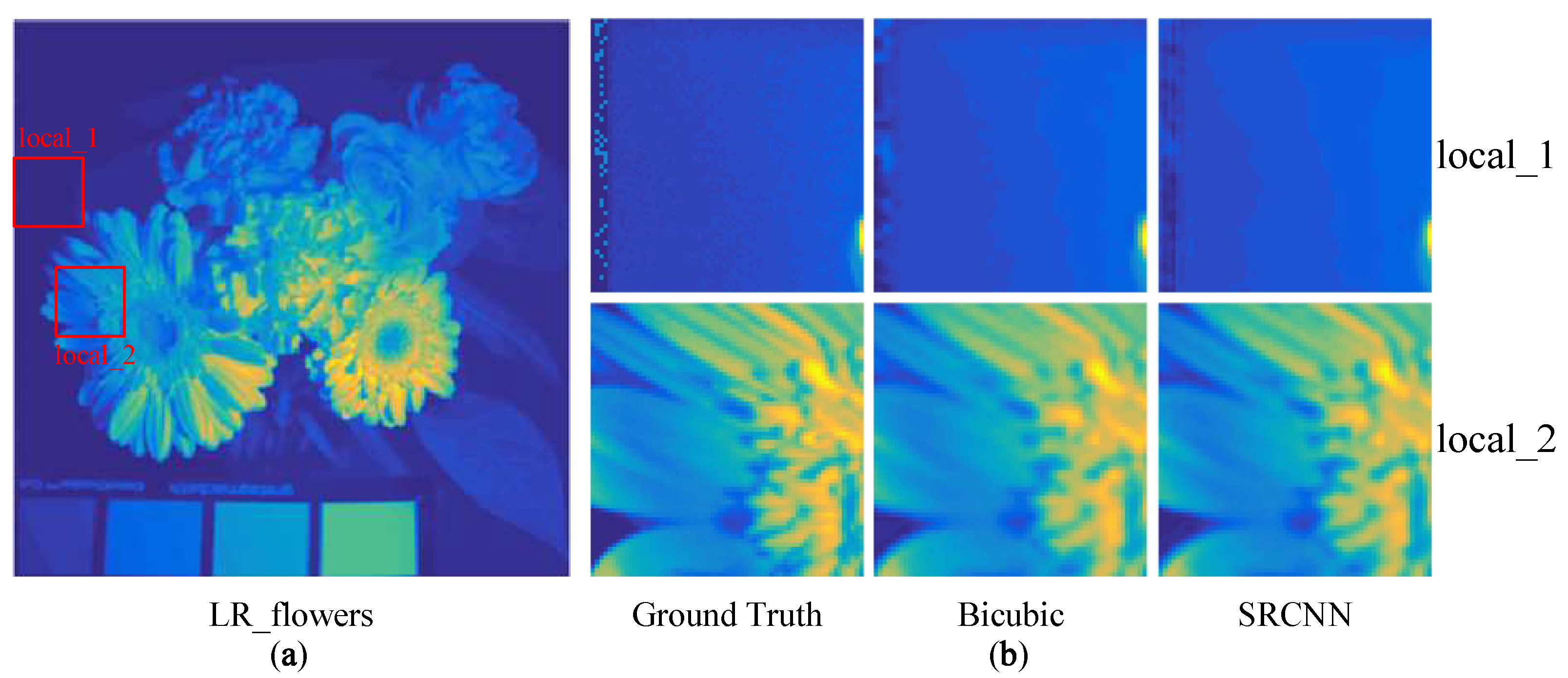
Meanwhile, experiments have also been conducted to validate the effectiveness of the gating mechanism. The HSI named as “flowers” in the CAVE dataset has been employed for this validation. A comparison is made between the HSIs reconstructed by the SRCNN and the bicubic methods. As shown in Figure 4a, the “LR_flowers” denotes a down-scaled LR HSI by the ratio of 0.5. Two rectangle regions are manually selected, which are marked with ’local_1’ and ’local_2’. The ’local_1’ and ’local_2’ regions denote the areas with poor and rich spatial information, respectively. There are three columns in Figure 4b, which visually displays the ground truth, the bicubic reconstructed area and the SRCNN reconstructed area. It is noticed that for the ‘local_1’ area with a homogeneous background, the classical bicubic method can easily achieve an acceptable performance. As to the ‘local_2’ area with more texture, both the SRCNN reconstructed and the bicubic reconstructed areas exhibit blurs between the neighboring petals. However, the information brought by the bicubic method is far less than that brought by the SRCNN, leading to its poor performance on the complex textures, such as the left-top regions of ’local_2’.

To further validate this observation, the PSNR, SSIM and SAM have been employed to conduct a quantitative evaluation. The results have been displayed in

Table 2. Quantitative evaluation of two different regions on ‘flower’.

	Metrics	PSNR	SSIM	SAM
local_1	Bicubic	51.2249	0.9905	5.4049
	SRCNN	50.425	0.9884	6.1364
local_2	Bicubic	39.4046	0.9716	1.6741
	SRCNN	40.2666	0.9729	2.4394

. The data in the first row of Table 2 have validated that the bicubic method outperforms the SRCNN in all the measurements when super-resolving the ‘local_1’ area. It demonstrates the effectiveness of the classical bicubic method for the homogeneous areas. On the other hand, the data in the last row of the Table 2 have proved the effectiveness of SRCNN for the areas with rich information. In this way, it is rational to incorporate the gating mechanism in the proposed GCoRDN to further improve the super-resolving performance.

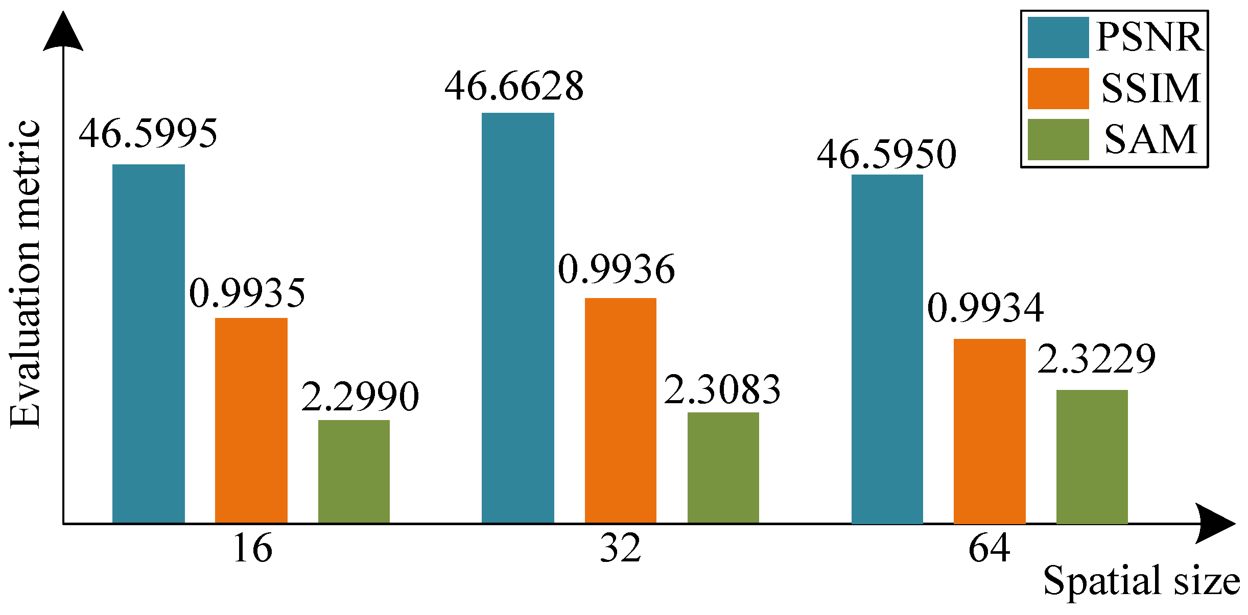
Meanwhile, it is mentioned in Section 2.4 that there is an all-zero tensor $\mathcal{T}$ manually formulated to make an evaluation of the information richness, whose size is $k\times k\times b$. k has ranged from 16 and 32 to 64 and to find the optimal size. The corresponding reconstruction performance of the GCoRDN on the CAVE dataset at the scaling factor of 2 is listed in Figure 5. The data in Figure 5 have shown that both the PSNR and SSIM obtain the optimal values when k is 32. The SAM is comparatively stable to the variation of the k. In this way, the k value is finally determined as 32 in the GM module. In this way, to make the proposed method more practical, the k is fixed as 32 for all the experimental data.

3.5. Ablation Study

To verify the effectiveness of key modules, this section tests variant versions of the proposed model by removing each component on the Cave dataset.

Table 3. Ablation experiments of different modules at the scaling factor 2 for the Cave dataset.

Module	Different Combinations of Modules
COC	✗	✔	✔	✔	✔
RDSAB	✔	✗	✔	✔	✔
Weight sharing	✔	✔	✗	✔	✔
GM	✔	✔	✔	✗	✔
PSNR	45.9308	46.4784	46.5884	46.4915	46.6628
SAM	2.3373	2.2571	2.2767	2.3977	2.3083
ERGAS	3.1426	3.0214	2.9795	2.9578	2.9395

shows the ablation study for key modules. Specifically, to validate the effectiveness of the COC module, the concatenation operation between the S, T, and the LR image was excluded, and the comparison of PSNR and SAM values between the first column and the last column proves that the introduction of the COC module can effectively avoid the problem of information loss in the process of structure extraction. The ablation experiment regarding the RDSAB module involves replacing the SA strategy with the RDB module, which proves that the module can improve the image spatial quality comparing with the last column. Then, we also conduct the experiment without weight sharing, which is to generate texture feature weights and structure feature weights separately in the attention mechanism of RDSAB. Table 3 demonstrates the effectiveness of adopting this strategy. Compared with the last column, the fourth column verifies that the GM module can further improve the network performance as a type of post-processing.

One can observe that the proposed combination produces better performance than any other arbitrary module combination, especially achieving the highest value in PSNR which measures the reconstruction ability of the methods. However, the SAM metric performs better without the inclusion of RDSAB module and weight sharing, indicating that these modules may introduce noise or uncertainty of the spectrum during the spatial reconstruction process. At the same time, using these modules significantly improves the PSNR and ERGAS metrics. Improvement of the PSNR indicates that the spatial information is enhanced by these modules. Meanwhile, better ERGAS values show that the spatial enhancement suppressed the spectral uncertainly brought by these modules. Overall, these modules can extract and retain more useful feature information, thereby enhancing the overall image quality and detail reconstruction ability.

4. Disscusion

4.1. Cave Dataset

To conduct a fair evaluation of the proposed GCoRDN, the pioneering deep learning-based HSI SR method, SRCNN [57], has been applied as one of the competitors. Because the baseline of the proposed method is the RDN, the RDN is also applied as one of the competitors. Meanwhile, two other extensions of the RDN, including the G-RDN and RSTDN, are also applied for the comparison. To demonstrate the superiority of our proposed model, the latest models SFCSR and ERCSR were also included in the comparative experiments. Due to GPU memory limitations, the number of modules in ERCSR was adjusted to 1. In addition, the classical bicubic is applied in the comparison.

Table 4. Average evaluation metrics for the Cave dataset.

Scaling Factor	Metrics	Bicubic	SRCNN	RDN	G-RDN	RSTDN	SFCSR	ERCSR	GCoRDN
2x	PSNR	42.5489	43.4588	44.8489	44.9913	45.0293	46.2606	46.0864	46.6628
	SSIM	0.9896	0.9877	0.9905	0.9909	0.9910	0.9928	0.9937	0.9936
	SAM	2.3344	3.2324	2.8657	2.7688	2.7771	3.4872	2.3244	2.3083
	ERGAS	4.6124	4.1068	3.5076	3.4674	3.4316	3.0806	3.1065	2.9395
3x	PSNR	38.8453	39.8498	40.3374	40.4575	40.4618	41.2759	41.1293	41.9424
	SSIM	0.9788	0.9781	0.9815	0.9819	0.9802	0.9858	0.9860	0.9858
	SAM	2.8973	3.6033	3.378	3.2557	3.5175	3.3984	2.5214	2.6283
	ERGAS	4.6447	4.1723	3.9569	3.8894	3.8639	3.6114	3.6619	3.3405
4x	PSNR	36.7106	38.1703	38.8653	38.6438	38.5754	39.4022	39.2211	39.6767
	SSIM	0.9676	0.9689	0.9716	0.9697	0.9703	0.9971	0.9766	0.9771
	SAM	3.4404	4.3295	4.1922	5.0645	4.267	3.3940	3.5259	3.3496
	ERGAS	4.444	3.7863	3.5043	3.5901	3.6415	3.3268	3.3974	3.3118

Note: The optimal and second optimal values have been highlighted by the bold format and the underline format, respectively.

lists the average quantitative evaluations on the CAVE dataset at different scaling factors. The best indices are highlighted in a bold format. The second optimal measurements are highlighted by the underline format. According to the data in Table 4, the proposed GCoRDN outperforms the other competitors in terms of the PSNR and ERGAS at the scaling factors of 2, 3 and 4. These two metrics are mainly utilized to evaluate the spatial quality and the overall quality of the reconstructed images, respectively. In this way, it is rational to say that the proposed method is effective in reconstructing the spatial detail and achieves an acceptable overall reconstruction ability. As for the remaining SSIM and SAM, the proposed method still achieves the optimal or suboptimal values. At the scaling factor of 4, the proposed GCoRDN outperforms the SRCNN and RDN by 1.5064 db and 0.8114 db, respectively. Meanwhile, even though the G-RDN imports the gradient information during the reconstruction process, the proposed GCoRDN still outperforms it, which make a further validation of the effectiveness of the proposed method. Furthermore, different from the RSTDN, the COC module, RDSABs and gating mechanism modules in the GCoRDN have ensured a further improvement of the reconstruction performance. In addition, a performance comparison between the GCoRDN and the GCoRDN without the gating mechanism (which are marked by the upper script *) is given in

Table 5. Average evaluation metrics achieved by the GCoRDN* and GCoRDN for the Cave dataset.

Scaling Factor	Method	PSNR	SSIM	SAM	ERGAS
2x	GCoRDN*	46.4915	0.9932	2.3977	2.9578
	GCoRDN	46.6628	0.9936	2.3083	2.9395
3x	GCoRDN*	41.7825	0.9852	2.7305	3.358
	GCoRDN	41.9424	0.9858	2.6283	3.3405
4x	GCoRDN*	39.6542	0.9763	3.4548	3.2997
	GCoRDN	39.6767	0.9771	3.3496	3.3118

. It is noted that the GCoRDN outperforms the GCoRDN* on almost all the measurements, which validated the effectiveness of the gating mechanism. Meanwhile, by combining the Table 4 and Table 5, it is noted that the GCoRDN* still outperforms most of the other methods, which further proves the effectiveness of the other two modules.

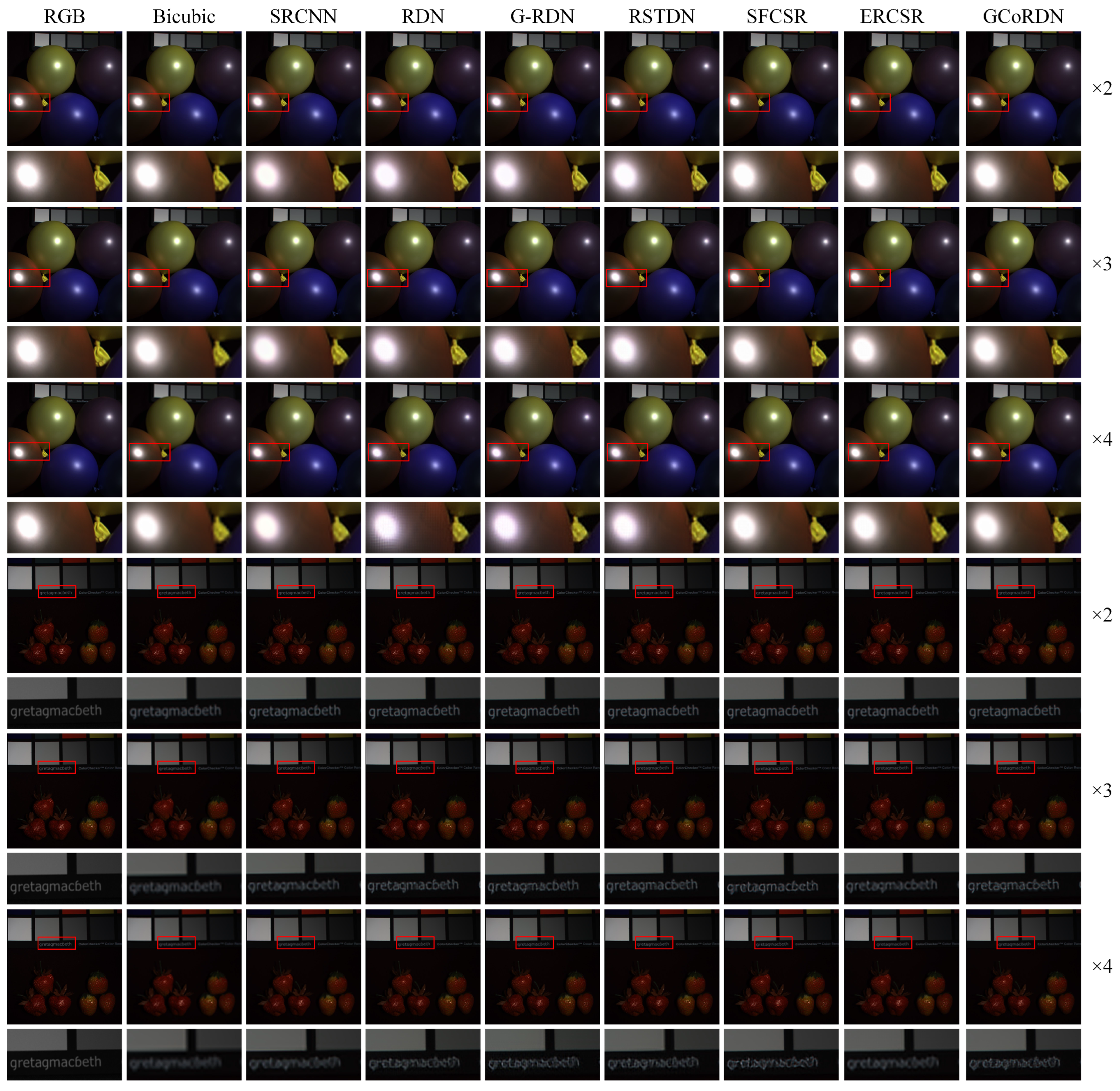
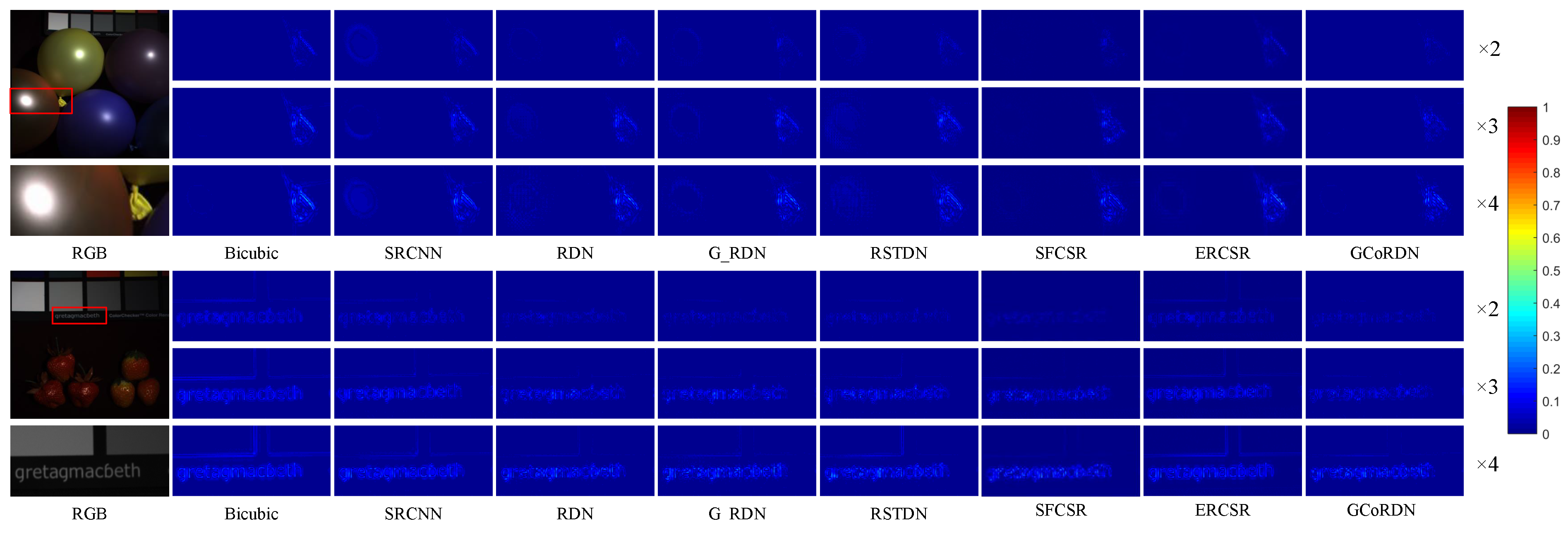
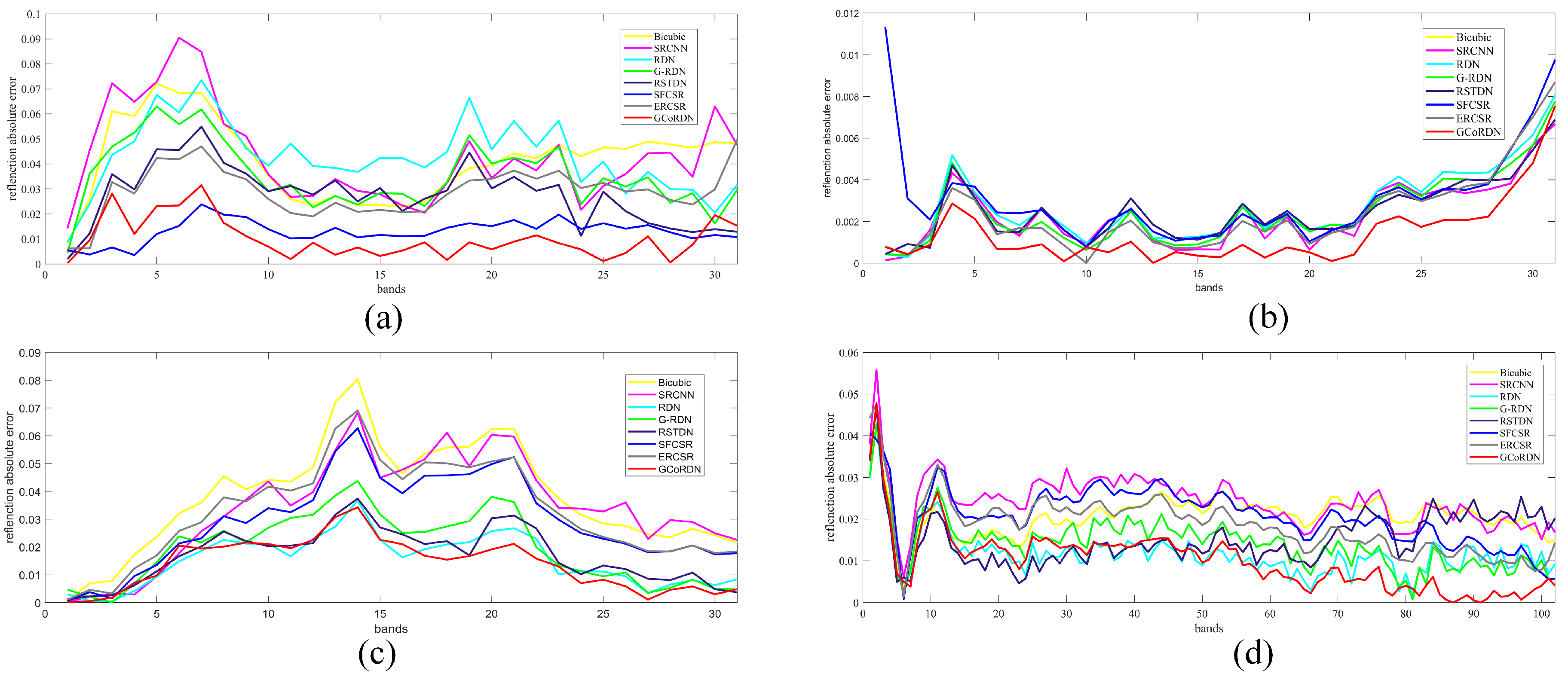
Figure 6 exhibits the visual exhibition of the reconstructed fake_and_real_strawberries and balloons. It should be noted that the RGB versions are composed by the 10th, 20th and 30th band in the reconstructed HSIs. A rectangle region with comparative rich texture has been selected from the reconstructed HSIs and amplified to make a better visual difference. For the balloons, it is noted that the ridge between the red balloon and the yellow one in the HSI reconstructed by the proposed method is the sharpest. As for the fake_and_real_strawberries, the letters reconstructed by the proposed method are still the clearest. The absolute error map of the proposed method in Figure 7 is closest to the dark blue. Figure 8a,b presents the spectral reconstruction error of one randomly selected pixel from each of the reconstructed HSIs. The curves reconstructed by the proposed method are closest to the x-axis, which demonstrates the effectiveness of the GCoRDN in preserving the spectral information for the CAVE dataset.

4.2. Harvard Dataset

The objective measurements on the Harvard dataset are listed in

Table 6. Average evaluation metrics for the Harvard dataset.

Scaling Factor	Metrics	Bicubic	SRCNN	RDN	G-RDN	RSTDN	SFCSR	ERCSR	GCoRDN
2x	PSNR	47.8050	48.2568	49.6857	49.3426	49.5636	49.3676	49.1446	49.5270
	SSIM	0.9940	0.9936	0.9948	0.9944	0.9948	0.9970	0.9969	0.9950
	SAM	1.7897	2.036	1.8656	1.9525	1.8433	2.1972	2.1927	1.8118
	ERGAS	3.8536	4.2734	4.0610	4.3104	4.0375	3.5580	3.5813	3.7823
3x	PSNR	45.2523	46.1117	46.4675	46.3401	46.4960	46.6199	46.1555	46.7033
	SSIM	0.9906	0.9912	0.9914	0.9908	0.9915	0.9921	0.9945	0.9921
	SAM	1.9576	2.1091	2.1550	2.2042	2.1386	2.6486	2.4997	2.0745
	ERGAS	3.0893	3.1778	3.2630	3.6983	3.2793	2.7905	2.4997	3.0862
4x	PSNR	43.774	44.4394	44.6581	44.4795	44.6474	44.4837	44.2345	44.6773
	SSIM	0.9876	0.9882	0.9882	0.9864	0.9883	0.9922	0.9919	0.9888
	SAM	2.0527	2.1787	2.3291	2.4642	2.3438	2.6486	2.6845	2.1795
	ERGAS	2.6169	2.6389	3.0183	3.7425	2.9889	2.7905	2.4294	2.6652

. Different from the HSIs in the CAVE dataset, which are captured in an indoor environment, many details of the HSIs in this dataset are obscured by the outdoor dark light, resulting in their poor spatial information. According to the data in Table 6, it is noticeable that the proposed GCoRDN achieves the optimal PSNR at the scaling factor of 3 and 4. When it comes to the overall metric ERGAS, the ERCSR obtains the optimal values. However, both SFCSR and the ERCSR adopt the weight-sharing strategy for the whole reconstruction process in the network, making the memory occupation linearly correlated with the number of the bands. In this way, for the HSIs with hundreds of bands, the reconstruction processed by the SFCSR and ERCSR requires a large amount of memory. The proposed GCoRDN super-resolves the entire HSI simultaneously, even though there is a weight sharing for the attention mechanism. In this way, the proposed method achieves a comparable reconstruction performance with the limited computational memory. Meanwhile, it is noted that the superiority of the deep learning-based methods over the classical bicubic methods is shrinking as the scaling factor grows. The main reason is that for a large scaling factor, the input image is down-sampled via a larger factor in correspondence, making the input LR HSIs convey less information. In this way, less information can be utilized for the deep learning-based methods, and the classical bicubic method exhibits a more stable performance. This further validates the rationality of the gating mechanism applied in the proposed method.

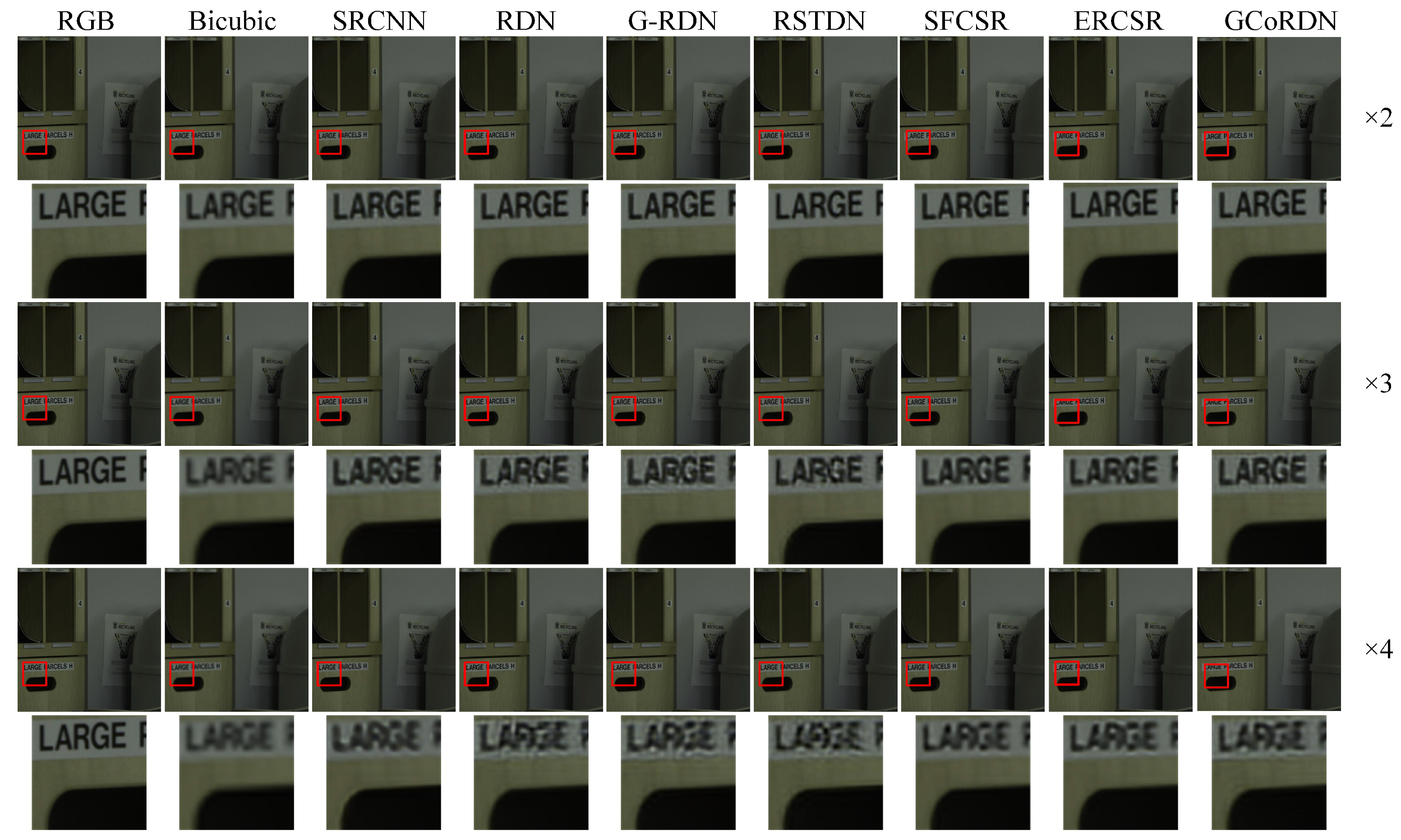
To evaluate the perceptual quality, Figure 9 shows the super-resolved output of the test HSI from the Harvard dataset and enlarges the same area marked by the red rectangle to show in detail. All deep methods exhibit the appealing spatial ability. In addition, the difference images between the ground truth HSI and the reconstructed ones have also been visually displayed in Figure 10. A square region of discriminable edges and structures in the scene is amplified to highlight the visual difference. It is observed that at the scaling factor of 2, all the reconstructed methods exhibit the acceptable performance, in which all the difference images are blue, and people cannot visually recognize the word ‘LARGE’ in the scene. As the scaling factor grows, the profiles of the word gradually become clearer. At a scaling factor of 3 and 4, it can be observed that the proposed method shows shallower edges or even no edges compared to other methods. This indicates that our method is capable of effectively restoring structural information, and it implies that our approach can maintain detailed information while also preventing excessive sharpening of the image. Spectrally, one pixel is randomly selected from the scene to show the spectral distortion in Figure 8c. For the selected point, the proposed method outperforms the other methods in the spectral preservation ability.

4.3. Pavia Center

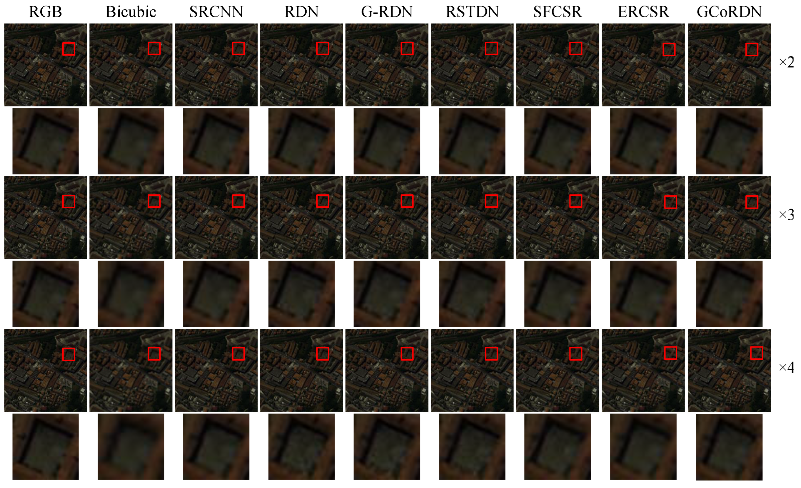
To enable a comprehensive performance evaluation of the proposed GCoRDN method, experiments have been also conducted on the airborne HSI named Pavia center with the least spatial information among the three datasets.

Table 7. Average evaluation metrics for the Pavia center.

Scaling Factor	Metrics	Bicubic	SRCNN	RDN	G-RDN	RSTDN	SFCSR	ERCSR	GCoRDN
2x	PSNR	32.8297	35.5476	36.0851	36.0548	36.1165	35.0796	35.4397	36.4866
	SSIM	0.903	0.9371	0.9406	0.9405	0.9418	0.9369	0.9402	0.9458
	SAM	3.935	3.6367	3.6671	3.6719	3.61213	3.6147	3.4202	3.5471
	ERGAS	8.3075	6.2692	5.9827	6.0043	5.9342	6.3559	6.2318	5.7479
3x	PSNR	29.6889	31.5700	31.6415	31.6342	31.6370	30.8804	31.2587	32.1459
	SSIM	0.8137	0.8642	0.8605	0.8576	0.8618	0.8519	0.8609	0.8768
	SAM	4.9308	4.5439	4.7506	5.0094	4.8279	5.0643	4.6435	4.6070
	ERGAS	7.7490	6.3153	6.2967	6.3190	6.2776	6.6824	6.5141	5.9961
4x	PSNR	27.9970	29.4344	29.1472	29.1928	29.1990	28.6395	29.1312	29.5475
	SSIM	0.7447	0.7992	0.7810	0.7763	0.7828	0.7675	0.7897	0.7953
	SAM	5.6473	5.2289	5.6593	5.8933	5.8525	6.1831	5.4685	5.5374
	ERGAS	6.9765	6.0061	6.1882	6.1712	6.1498	6.4272	6.1321	5.9374

and Figure 11, respectively, exhibit the quantitative and qualitative measurements of the reconstructed Pavia center. Table 7 exhibits the objective metrics of the reconstructed Pavia center. The proposed method still achieves the optimal PSNR and ERGAS. As for the SAM and SSIM, the proposed method achieves suboptimal values. At the scaling factor of 3, the SRCNN achieves the optimal SAM, which obtains a 0.06° priority over the proposed GCoRDN. However, the proposed GCoRDN surpasses the SRCNN with a PSNR improvement of nearly 0.6 db. The overall measurement ERGAS indicates the superiority of the proposed GCoRDN method. At the scaling factor of 4, the SRCNN still achieves the optimal SAM, besides the SSIM. Due to the adoption of a band grouping strategy, SFCSR and ERCSR did not exhibit satisfactory performance for the Pavia center with a large number of bands. However, the proposed GCoRDN still achieves the optimal ERGAS and PSNR.

Visually, presentations about the difference images reconstructed by different methods at different scaling factors are listed in Figure 11. Overall, it is noticed that the frame of the buildings in the selected area become clearer as the scaling factor increases. This demonstrates that as the scaling factor grows, the difference tends to become large, and the profile of the scene can gradually be noticed. The results of the spatial absolute error visualization are shown in Figure 12. To be specific, at the scaling factor of 3, the boundary of the buildings can be clearly seen in the difference images which are generated by the bicubic, SRCNN, RDN, SFCSR, ERCSR methods. Furthermore, the difference image generated by our method is the closest to dark blue when compared with the image reconstructed by the G-RDN and RSTDN methods. In this way, it is also illustrated that the proposed GCoRDN is effective in the airborne HSI as well as the ground-based HSIs. In addition, one pixel in Figure 8d was plotted to visually show the spectral difference. The randomly selected pixel by the proposed GCoRDN exhibits the strongest spectral preservation ability in all bands after the 60th band. For the remaining bands, GCoRDN continues to maintain a strong competitive performance.

In this way, experiments on both the ground-based HSIs and the airborne HSI have demonstrated the superiority of the proposed method at different scaling factors. Meanwhile, data analysis has proved the effectiveness the three modules designed in the GCoRDN.

5. Conclusions

This paper has presented a novel gated content-oriented residual dense network for HSI super-resolution. Inspired by the important observations that the texture and structure exhibit different sensitivities to the spatial resolution, this paper proposes a network with three modules to super-resolve the HSI, which makes a deep utilization of the content in the HSI. The structure and texture are dealt through two branches, which are followed by a weight-sharing spectral attention strategy. In addition, the gating mechanism is applied to further improve the HSIs. Experimental results and data analysis have demonstrated the superiority of the proposed method.

References

1. Li, J.; Zi, S.; Song, R.; Li, Y.; Hu, Y.; Du, Q. A Stepwise Domain Adaptive Segmentation Network With Covariate Shift Alleviation for Remote Sensing Imagery. IEEE Trans. Geosci. Remote Sens. 2022, 60, 1–15. [Google Scholar] [CrossRef]
2. Rasti, B.; Hong, D.; Hang, R.; Ghamisi, P.; Kang, X.; Chanussot, J.; Benediktsson, J.A. Feature Extraction for Hyperspectral Imagery: The Evolution From Shallow to Deep: Overview and Toolbox. IEEE Geosci. Remote Sens. Mag. 2021, 8, 60–88. [Google Scholar] [CrossRef]
3. Zheng, X.; Sun, H.; Lu, X.; Xie, W. Rotation-Invariant Attention Network for Hyperspectral Image Classification. IEEE Trans. Image Process. 2022, 31, 4251–4265. [Google Scholar] [CrossRef] [PubMed]
4. Huang, Q.; Li, W.; Zhang, B.; Li, Q.; Tao, R.; Lovell, N.H. Blood Cell Classification Based on Hyperspectral Imaging with Modulated Gabor and CNN. IEEE J. Biomed. Health Inform. 2020, 24, 160–170. [Google Scholar] [CrossRef]
5. Shimoni, M.; Haelterman, R.; Perneel, C. Hypersectral Imaging for Military and Security Applications: Combining Myriad Processing and Sensing Techniques. IEEE Geosci. Remote Sens. Mag. 2019, 7, 101–117. [Google Scholar] [CrossRef]
6. Li, Y.; Ren, J.; Yan, Y.; Liu, Q.; Ma, P.; Petrovski, A.; Sun, H. CBANet: An End-to-End Cross-Band 2-D Attention Network for Hyperspectral Change Detection in Remote Sensing. IEEE Trans. Geosci. Remote Sens. 2023, 61, 1–11. [Google Scholar] [CrossRef]
7. Zheng, X.; Chen, X.; Lu, X.; Sun, B. Unsupervised Change Detection by Cross-Resolution Difference Learning. IEEE Trans. Geosci. Remote Sens. 2022, 60, 1–16. [Google Scholar] [CrossRef]
8. Li, J.; Leng, Y.; Song, R.; Liu, W.; Li, Y.; Du, Q. MFormer: Taming Masked Transformer for Unsupervised Spectral Reconstruction. IEEE Trans. Geosci. Remote Sens. 2023, 61, 1–12. [Google Scholar] [CrossRef]
9. Arias, F.; Zambrano, M.; Broce, K.; Medina, C.; Pacheco, H.; Nunez, Y. Hyperspectral imaging for rice cultivation: Applications, methods and challenges. AIMS Agric. Food 2021, 6, 273–307. [Google Scholar] [CrossRef]
10. Dian, R.; Li, S.; Sun, B.; Guo, A. Recent advances and new guidelines on hyperspectral and multispectral image fusion. Inf. Fusion 2021, 69, 40–51. [Google Scholar] [CrossRef]
11. Hao, S.; Wang, W.; Ye, Y.; Li, E.; Bruzzone, L. A deep network architecture for super-resolution-aided hyperspectral image classification with classwise loss. IEEE Trans. Geosci. Remote Sens. 2018, 56, 4650–4663. [Google Scholar] [CrossRef]
12. Hu, J.; Li, Y.; Xie, W. Hyperspectral image super-resolution by spectral difference learning and spatial error correction. IEEE Geosci. Remote Sens. Lett. 2017, 14, 1825–1829. [Google Scholar] [CrossRef]
13. Dian, R.; Li, S.; Kang, X. Regularizing hyperspectral and multispectral image fusion by CNN denoiser. IEEE Trans. Neural Netw. Learn. Syst. 2021, 32, 1124–1135. [Google Scholar] [CrossRef] [PubMed]
14. Ma, Q.; Jiang, J.; Liu, X.; Ma, J. Deep Unfolding Network for Spatiospectral Image Super-Resolution. IEEE Trans. Comput. Imaging 2022, 8, 28–40. [Google Scholar] [CrossRef]
15. Yokoya, N.; Grohnfeldt, C.; Chanussot, J. Hyperspectral and multispectral data fusion: A comparative review of the recent literature. IEEE Geosci. Remote Sens. Mag. 2017, 5, 29–56. [Google Scholar] [CrossRef]
16. Yan, L.; Wang, X.; Zhao, M.; Kaloorazi, M.; Chen, J.; Rahardja, S. Reconstruction of hyperspectral data from RGB images with prior category information. IEEE Trans. Comput. Imaging 2020, 6, 1070–1081. [Google Scholar] [CrossRef]
17. Wang, X.; Chen, J.; Wei, Q.; Richard, C. Hyperspectral Image Super-Resolution via Deep Prior Regularization with Parameter Estimation. IEEE Trans. Circuits Syst. Video Technol. 2022, 32, 1708–1723. [Google Scholar] [CrossRef]
18. Qu, J.; Hou, S.; Dong, W.; Xiao, S.; Du, Q.; Li, Y. A Dual-Branch Detail Extraction Network for Hyperspectral Pansharpening. IEEE Trans. Geosci. Remote Sens. 2022, 60, 1–13. [Google Scholar] [CrossRef]
19. Li, J.; Zheng, K.; Yao, J.; Gao, L.; Hong, D. Deep Unsupervised Blind Hyperspectral and Multispectral Data Fusion. IEEE Geosci. Remote Sens. Lett. 2022, 19, 1–5. [Google Scholar] [CrossRef]
20. Xie, W.; Lei, J.; Cui, Y.; Li, Y.; Du, Q. Hyperspectral Pansharpening With Deep Priors. IEEE Trans. Neural Netw. Learn. Syst. 2020, 31, 1529–1543. [Google Scholar] [CrossRef]
21. Dong, W.; Zhang, T.; Qu, J.; Xiao, S.; Liang, J.; Li, Y. Laplacian pyramid dense network for hyperspectral pansharpening. IEEE Trans. Geosci. Remote Sens. 2022, 60, 5507113. [Google Scholar] [CrossRef]
22. Li, S.; Tian, Y.; Xia, H.; Liu, Q. Unmixing based PAN guided fusion network for hyperspectral imagery. IEEE Trans. Geosci. Remote Sens. 2022, 60, 5522017. [Google Scholar] [CrossRef]
23. Sun, W.; Ren, K.; Meng, X.; Yang, G.; Xiao, C.; Peng, J.; Huang, J. MLR-DBPFN: A Multi-Scale Low Rank Deep Back Projection Fusion Network for Anti-Noise Hyperspectral and Multispectral Image Fusion. IEEE Trans. Geosci. Remote Sens. 2022, 60, 1–14. [Google Scholar] [CrossRef]
24. Huang, T.; Dong, W.; Wu, J.; Li, L.; Li, X.; Shi, G. Deep Hyperspectral Image Fusion Network With Iterative Spatio-Spectral Regularization. IEEE Trans. Comput. Imaging 2022, 8, 201–214. [Google Scholar] [CrossRef]
25. Xie, Q.; Zhou, M.; Zhao, Q.; Xu, Z.; Meng, D. MHF-net: An interpretable deep network for multispectral and hyperspectral image fusion. IEEE Trans. Pattern Anal. Mach. Intell. 2022, 44, 1457–1473. [Google Scholar] [CrossRef] [PubMed]
26. He, W.; Chen, Y.; Yokoya, N.; Li, C.; Zhao, Q. Hyperspectral super-resolution via coupled tensor ring factorization. Pattern Recognit. 2022, 122, 108280. [Google Scholar] [CrossRef]
27. Fu, H.; Sun, G.; Zhang, A.; Shao, B.; Ren, J.; Jia, X. Tensor Singular Spectral Analysis for 3D feature extraction in hyperspectral images. IEEE Trans. Geosci. Remote Sens. 2023, 61, 1. [Google Scholar] [CrossRef]
28. Xu, Y.; Wu, Z.; Chanussot, J.; Wei, Z. Hyperspectral Images Super-Resolution via Learning High-Order Coupled Tensor Ring Representation. IEEE Trans. Neural Netw. Learn. Syst. 2020, 31, 4747–4760. [Google Scholar] [CrossRef] [PubMed]
29. Wang, X.; Ma, J.; Jiang, J. Hyperspectral Image Super-Resolution via Recurrent Feedback Embedding and Spatial–Spectral Consistency Regularization. IEEE Trans. Geosci. Remote Sens. 2022, 60, 1–16. [Google Scholar] [CrossRef]
30. Sun, G.; Fu, H.; Ren, J.; Zhang, A.; Zabalza, J.; Jia, X.; Zhao, H. SpaSSA: Superpixelwise Adaptive SSA for Unsupervised Spatial-Spectral Feature Extraction in Hyperspectral Image. IEEE Trans. Cybern. 2022, 52, 6158–6169. [Google Scholar] [CrossRef]
31. Dong, L.; Yuan, Y.; Luxs, X. Spectral–spatial joint sparse NMF for hyperspectral unmixing. IEEE Trans. Geosci. Remote Sens. 2021, 59, 2391–2402. [Google Scholar] [CrossRef]
32. Zhang, Y.; Wang, T.; Mei, S.; Du, Q. Subpixel Mapping of Hyperspectral Images Using a Labeled-Unlabeled Hybrid Endmember Library and Abundance Optimization. IEEE J. Sel. Top. Appl. Earth Obs. Remote Sens. 2020, 13, 5036–5047. [Google Scholar] [CrossRef]
33. He, D.; Zhong, Y.; Wang, X.; Zhang, L. Deep convolutional neural network framework for subpixel mapping. IEEE Trans. Geosci. Remote Sens. 2021, 59, 9518–9539. [Google Scholar] [CrossRef]
34. Mei, S.; Yuan, X.; Ji, J.; Zhang, Y.; Wan, S.; Du, Q. Hyperspectral Image Spatial Super-Resolution via 3D Full Convolutional Neural Network. Remote Sens. 2017, 9, 1139. [Google Scholar] [CrossRef] [Green Version]
35. Hu, J.; Jia, X.; Li, Y.; He, G.; Zhao, M. Hyperspectral Image Super-Resolution via Intrafusion Network. IEEE Trans. Geosci. Remote Sens. 2020, 58, 7459–7471. [Google Scholar] [CrossRef]
36. Li, Q.; Wang, Q.; Li, X. Mixed 2D/3D Convolutional Network for Hyperspectral Image Super-Resolution. Remote Sens. 2020, 12, 1660. [Google Scholar] [CrossRef]
37. Zhao, M.; Ning, J.; Hu, J.; Li, T. Hyperspectral Image Super-Resolution under the Guidance of Deep Gradient Information. Remote Sens. 2021, 13, 2382. [Google Scholar] [CrossRef]
38. Hu, J.; Li, T.; Zhao, M.; Ning, J. Hyperspectral Image Superresolution via Deep Structure and Texture Interfusion. IEEE J. Sel. Top. Appl. Earth Obs. Remote Sens. 2021, 14, 8665–8678. [Google Scholar] [CrossRef]
39. Wang, Q.; Li, Q.; Li, X. Hyperspectral Image Superresolution Using Spectrum and Feature Context. IEEE Trans. Ind. Electron. 2021, 68, 11276–11285. [Google Scholar] [CrossRef]
40. Li, Q.; Wang, Q.; Li, X. Exploring the Relationship Between 2D/3D Convolution for Hyperspectral Image Super-Resolution. IEEE Trans. Geosci. Remote Sens. 2021, 59, 8693–8703. [Google Scholar] [CrossRef]
41. Li, J.; Liu, Y.; Song, R.; Li, Y.; Han, K.; Du, Q. Sal2RN: A Spatial-Spectral Salient Reinforcement Network for Hyperspectral and LiDAR Data Fusion Classification. IEEE Trans. Geosci. Remote Sens. 2023, 61, 1–14. [Google Scholar] [CrossRef]
42. Li, J.; Ma, Y.; Song, R.; Xi, B.; Hong, D.; Du, Q. A Triplet Semisupervised Deep Network for Fusion Classification of Hyperspectral and LiDAR Data. IEEE Trans. Geosci. Remote Sens. 2022, 60, 1–13. [Google Scholar] [CrossRef]
43. Li, J.; Du, S.; Song, R.; Wu, C.; Li, Y.; Du, Q. HASIC-Net: Hybrid Attentional Convolutional Neural Network With Structure Information Consistency for Spectral Super-Resolution of RGB Images. IEEE Trans. Geosci. Remote Sens. 2022, 60, 1–15. [Google Scholar] [CrossRef]
44. Zheng, X.; Chen, W.; Lu, X. Spectral Super-Resolution of Multispectral Images Using Spatial-Spectral Residual Attention Network. IEEE Trans. Geosci. Remote Sens. 2022, 60, 1–14. [Google Scholar] [CrossRef]
45. Zheng, X.; Chen, X.; Lu, X. Visible-Infrared Person Re-Identification via Partially Interactive Collaboration. IEEE Trans. Image Process. 2022, 31, 6951–6963. [Google Scholar] [CrossRef]
46. Ning, H.; Zheng, X.; Lu, X.; Yuan, Y. Disentangled Representation Learning for Cross-Modal Biometric Matching. IEEE Trans. Multimed. 2022, 24, 1763–1774. [Google Scholar] [CrossRef]
47. Ding, K.; Ma, K.; Wang, S.; Simoncelli, E.P. Image Quality Assessment: Unifying Structure and Texture Similarity. IEEE Trans. Pattern Anal. Mach. Intell. 2022, 44, 2567–2581. [Google Scholar] [CrossRef] [PubMed]
48. Xu, L.; Yan, Q.; Xia, Y.; Jia, J. Structure Extraction from Texture via Relative Total Variation. ACM Trans. Graph. 2012, 31, 1–10. [Google Scholar] [CrossRef] [Green Version]
49. Zheng, X.; Zhang, Y.; Zheng, Y.; Luo, F.; Lu, X. Abnormal event detection by a weakly supervised temporal attention network. CAAI Trans. Intell. Technol. 2022, 7, 419–431. [Google Scholar] [CrossRef]
50. Zheng, X.; Wang, B.; Du, X.; Lu, X. Mutual Attention Inception Network for Remote Sensing Visual Question Answering. IEEE Trans. Geosci. Remote Sens. 2022, 60, 1–14. [Google Scholar] [CrossRef]
51. Wang, Q.; Li, Q.; Li, X. A fast neighborhood grouping method for hyperspectral band selection. IEEE Trans. Geosci. Remote Sens. 2021, 59, 5028–5039. [Google Scholar] [CrossRef]
52. Zhang, Y.; Tian, Y.; Kong, Y.; Zhong, B.; Fu, Y. Residual Dense Network for Image Super-Resolution. In Proceedings of the 2018 IEEE/CVF Conference on Computer Vision and Pattern Recognition, Salt Lake City, UT, USA, 18–23 June 2018; pp. 2472–2481. [Google Scholar] [CrossRef] [Green Version]
53. Yasuma, F.; Mitsunaga, T.; Iso, D.; Nayar, S.K. Generalized Assorted Pixel Camera: Postcapture Control of Resolution, Dynamic Range, and Spectrum. IEEE Trans. Image Process. 2010, 19, 2241–2253. [Google Scholar] [CrossRef] [PubMed] [Green Version]
54. Chakrabarti, A.; Zickler, T. Statistics of Real-World Hyperspectral Images. In Proceedings of the IEEE Conference on Computer Vision and Pattern Recognition (CVPR), Colorado Springs, CO, USA, 20–25 June 2011; pp. 193–200. [Google Scholar]
55. Fauvel, M.; Tarabalka, Y.; Benediktsson, J.A.; Chanussot, J.; Tilton, J.C. Advances in Spectral-Spatial Classification of Hyperspectral Images. Proc. IEEE 2013, 101, 652–675. [Google Scholar] [CrossRef]
56. Lim, B.; Son, S.; Kim, H.; Nah, S.; Mu Lee, K. Enhanced deep residual networks for single image super-resolution. In Proceedings of the IEEE Conference on Computer Vision and Pattern Recognition Workshops, Honolulu, HI, USA, 21–26 July 2017; pp. 136–144. [Google Scholar]
57. Dong, C.; Loy, C.C.; He, K.; Tang, X. Image Super-Resolution Using Deep Convolutional Networks. IEEE Trans. Pattern Anal. Mach. Intell. 2016, 38, 295–307. [Google Scholar] [CrossRef] [Green Version]
Figure 1. Framework of the proposed GCoRDN.
Remotesensing 15 03378 g001
Figure 2. Architecture of the RDB.
Remotesensing 15 03378 g002
Figure 3. The attention mechanism inside the RDSAB.
Remotesensing 15 03378 g003
Figure 4. (a): LR_flowers; (b): Visual exhibition of two different regions in the reconstructed flowers via the bicubic and the SRCNN method.
Remotesensing 15 03378 g004
Figure 5. Performance of parameter k with different values.
Remotesensing 15 03378 g005
Figure 6. Visual exhibition on two selected test images of the Cave dataset.
Remotesensing 15 03378 g006
Figure 7. Absolute error map comparisons on two selected test images of the Cave dataset.
Remotesensing 15 03378 g007
Figure 8. Spectral curves in the reconstructed different dataset with scale with ×2. (a,b) Cave dataset. (c) Harvard dataset. (d) Pavia center.
Remotesensing 15 03378 g008
Figure 9. Visual exhibition on Harvard dataset.
Remotesensing 15 03378 g009
Figure 10. Absolute error map comparisons on Harvard dataset.
Remotesensing 15 03378 g010
Figure 11. Visual exhibition on Pavia center.
Remotesensing 15 03378 g011
Figure 12. Absolute error map comparisons on Pavia Center.
Remotesensing 15 03378 g012