Abstract
Numerous works have explored deep models for the classification of high-resolution natural images. However, limited investigation has been made into a deep classification for low-resolution synthetic aperture radar (SAR) images, which is a challenging yet important task in the field of remote sensing. Existing work adopted ROC–VGG, which has a huge amount of parameters, thus limiting its application in practical deployment. It remains unclear whether the techniques developed in high-resolution natural images to make the model lightweight can be effective for low-resolution SAR images. Therefore, with prior work as the baseline, this work conducts an empirical study, testing three popular lightweight techniques: (1) channel attention module; (2) spatial attention module; (3) multi-stream head. Our empirical results show that these lightweight techniques in the high-resolution natural image domain can also be effective in the low-resolution SAR domain. We reduce the parameters from 9.2M to 0.17M while improving the performance from 94.8% to 96.8%.
1. Introduction
SAR based on electromagnetic scattering and coherence offers benefits over optical and infrared sensors as an active image sensor for detection and surveillance due to its capability of strong penetration [1,2,3,4]. As a result, it has numerous applications in both military and civilian domains, with classification being the most fundamental one. SAR images differ significantly from natural images due to the imaging technique, where the resolution of SAR images may vary for different scenarios, for example, in foliage-penetrating applications, where the carrier frequency of SAR is lower in order to penetrate canopies, resulting in low bandwidths in both range and cross-range directions. Therefore, foliage-penetrating SAR images have poor resolution, making the image classification more challenging. One existing study [5] for classification of foliage-penetrating SAR images proposed VGG powered by Receiver Operating Characteristic (ROC), with restricted performance and a large number of parameters.
In recent years, great progress has been made in the neural network-based classification of high-resolution natural images, which focuses on deep [6] and wide networks [7] to obtain good performance. Increasing the model depth yields a model that has a large number of parameters, making it difficult to deploy in many real-world applications. Therefore, numerous works [8,9,10] have paid careful attention to increase the model performance by adding negligible computation and parameter overhead. For example, SENet [8] introduces an attention module that automatically decides the weight for each channel to increase the model performance. On top of SENet, CBAM [9] additionally introduces a spatial attention module for further boosting the model performance. It is worth mentioning that channel attention module [8] and spatial attention module [9] do not increase the model width or depth; thus, they can be seen as an almost free boost. MGTS [11] proposes a simple yet effective method based on two streams for person search, with the two streams utilized for detection and re-identification feature extraction.
These models considerably improve performance in natural images while reducing parameters due to using these simple yet effective structures. In the computer vision community, new techniques are often developed on natural datasets. CNN structures, channel attention, and spatial attention have been widely shown to work well for natural datasets. However, it is worth mentioning that these techniques mainly improve the model performance from the architecture perspective instead of the dataset type. Intuitively, those techniques that can improve the performance of natural images are expected to improve the performance of low-resolution SAR images. Nonetheless, the effectiveness of those techniques in low-resolution SAR needs to be empirically validated. Our work fills this gap by applying these structures on low-resolution SAR image classification. The resolution for natural images often refers to the number of pixels in the image, while the resolution in SAR refers to the radar system’s ability to distinguish targets on the ground, specifically the minimum distance between two adjacent targets that can be identified. SAR resolution depends on several factors, including radar frequency, antenna size, antenna motion, and signal processing. Inspired by two-stream CNN [11], SENet [8], and CBAM [9], we offer an empirical study on the capability of CNN powered with multi-stream and attention modules for low-resolution SAR images, where attention-based multi-stream CNNs (AMS-CNNs) are proposed. AMS-CNN mainly consists of two components: the first one extracting low-level features, and the second one extracting high-level features. Specifically, this model focuses on two basic techniques for improving performance without significantly increasing parameters: attention modules and multi-stream heads. Two distinct domains of attention blocks, which belong to the first part of AMS-CNN, have the capability to select important low-level features that are beneficial for classification. The multi-steam head, including the maximum, median, and average features extractor, aims to obtain diverse high-level features. Moreover, considering the limited dataset in foliage-penetrating SAR images, DCGAN is used to generate synthetic SAR images to augment. We applied our proposed method to CARABAS-II foliage-penetrating SAR images presented in Figure 1, which achieved competitive performance with significantly lower performance than the baseline.
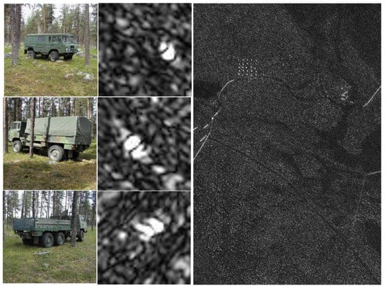
Figure 1.
Natural pictures for different vehicles and extracted SAR images. First column: natural pictures; second column: SAR images; third column: example image from the CARABAS-II SAR dataset; first row: TGB11; second row: TGB30; third row: TGB40.
The rest of this paper is organized as follows. Section 2 introduces related work by summarizing the progress of attention block and multi-stream in CNN for the SAR image classification and GAN for SAR image augmentation. Section 3 discusses the method and material, including the basic functions of CNN (Section 3.1), the attention mechanism (Section 3.2), the structure of AMS-CNN (Section 3.3), data generation with GAN (Section 3.4), and dataset (Section 3.5). Section 4 presents the results with GAN selection (Section 4.1), and experimental results of AMS-CNN, including comparative (Section 4.2), ablation (Section 4.3), and robustness (Section 4.4) experiments. Section 5 presents the discussion for this work.
2. Related Work
Attention in SAR image classification. The attention mechanism has been proposed due to the idea that it makes the model pay more attention to the key information. The attention mechanism can be classified as spatial, channel, layer, and mixed-domain based on the aspects of differently calculated domains. Numerous works [12,13,14,15] have applied attention modules to high-resolution SAR target recognition, which gain significant performance. The study [12] serves as a pioneering work, proposing a CNN architecture powered by attention modules, with a fully convolutional attention block (FCAB) containing a channel and spatial module. The two attention modules utilize average-pooling and max-pooling convolutional operations to extract complementary features. The results demonstrate that the proposed method improves performance significantly on the MSTAR dataset. AM-CNN [15] is built on the framework of A-ConvNets [16], with the fully connected layers eliminated and the convolutional layers remaining, each followed by a convolutional block attention module. Compared to A-ConvNets [16], the performance of this model improved, while the parameters were reduced by 5.12 M.
Muti-stream in SAR image classification. The concept of multi-stream is introduced to make the model pay greater attention to distinct features, thereby improving the performance of the model while decreasing the number of parameters. Numerous works [17,18,19] focus on utilizing multiple streams in high-resolution SAR images. MS-CNN [17] is composed of three layers, the first of which is a multi-stream convolutional layer that extracts multiple views of SAR images to obtain various features. The Fourier feature fusion and connected layers then follow. On the MSTAR dataset, experimental results show that the proposed method outperforms the others under both Standard Operating Conditions (SOC) and Extended Operating Conditions (EOC). Two-stream CNN [18] focuses on utilizing lightweight CNN to have a good performance on moving and stationary SAR datasets, with dramatically fewer parameters. Two streams and convolutional are utilized in two-stream CNN, where two streams have the capacity to extract local and global features, enabling the model to learn rich multilevel features. The experimental results have demonstrated that the proposed model has good performance on moving and stationary SAR datasets, with dramatically fewer parameters.
GAN for SAR image augmentation. Generative adversarial networks (GANs) [20] have been widely used for SAR image classification to augment data [21,22]. Ref. [23] adopted a multi-discriminator (MGAN) to generate synthetic images, which are then combined with real SAR images as CNN input. The results demonstrated that adding synthetic samples in training can increase the CNN classification accuracy, especially with the limited dataset. Moreover, in [24], a constrained naive GAN (CN-GAN) was presented, combing the properties of Least Squares Generative Networks (LSGAN) [25] and Image-to-Image Translation (Pix2Pix) [26] to stabilize the generative data. Its results demonstrated that the synthetic SAR images generated by CN-GAN have high quality. Simultaneously, the CNN with CN-GAN data augmentation performs better in classification accuracy.
3. Method and Material
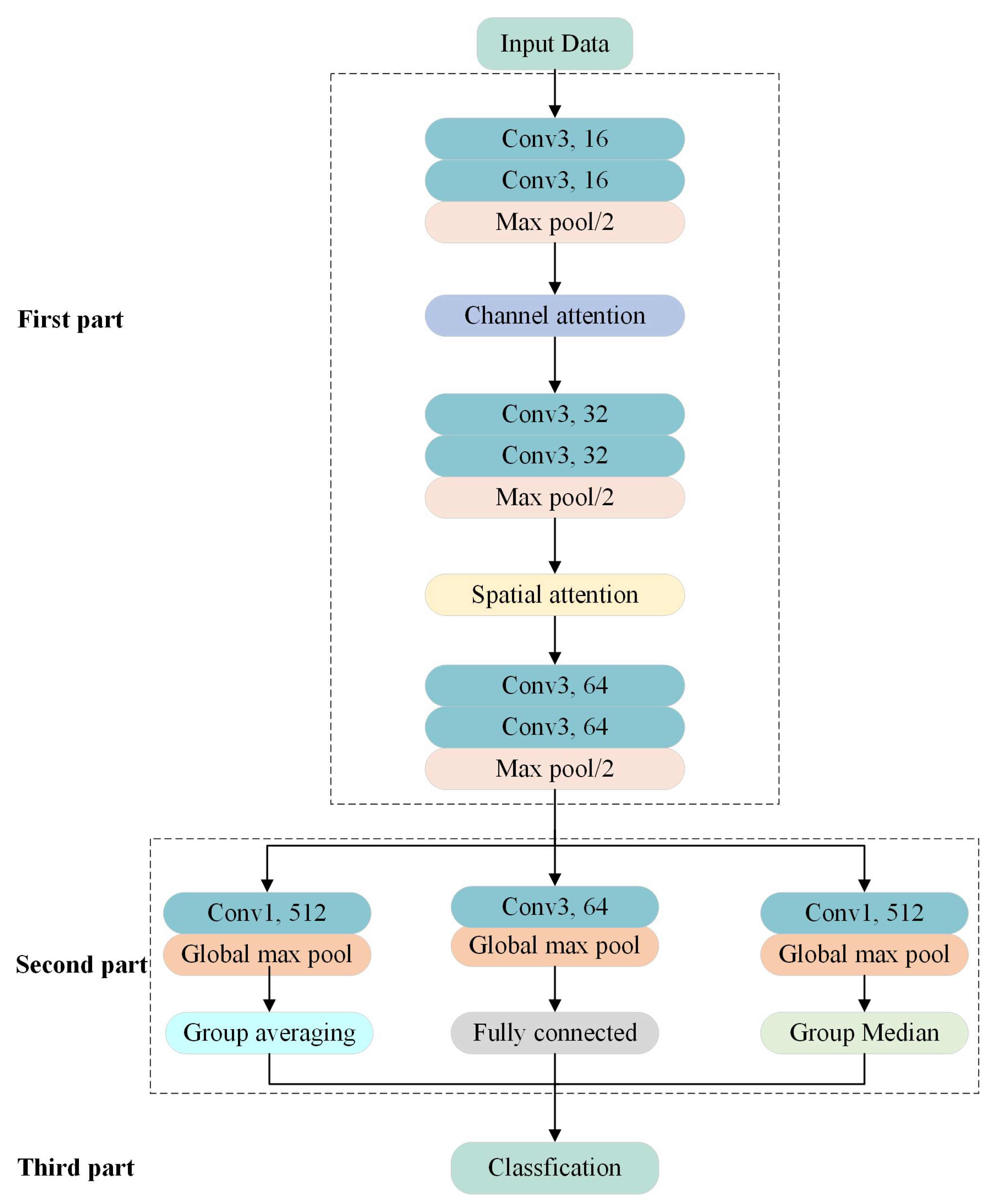
In this section, we introduce the lightweight CNN that we proposed for low-resolution SAR images in detail. We propose attention-based multi-stream convolutional neural networks (AMS-CNN) for SAR image classification by extracting key and diverse features, which is depicted in Figure 2. ASM-CNN includes three parts. On the one hand, the first section utilizes three convolutional blocks and pooling layers to extract low-level features, where each convolutional block has two convolutional layers with a different number of channels. The first part, on the other hand, utilizes two domains of attention blocks to focus on the important features, where the output of the attention module is the product between the input features and the attention features. The second part extracts various high-level characteristics (i.e., maximum, average, and median features) from three streams using varied strides and channels. Finally, the third part combines the features extracted by three streams for image classification, and the AMS-CNN output is the type of vehicle. Moreover, we explore the different GAN variants for foliage-penetrating SAR image generation.
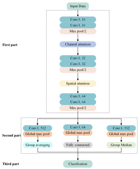
Figure 2.
AMS-CNN structure.
3.1. Basic Functions of CNN
In this section, we introduce the basic functions of CNN: the activation function, loss function, and dropout.
Activation Function. The activation function follows the convolution layer and is able to express the nonlinear mapping relationship between the input and output. Traditional nonlinear activation functions include double tangent and sigmoid. However, the gradient of these functions disappears in a certain range, which is not conducive to the training of the network. Recently, ReLU has attracted more attention for its good properties, which can obtain non-zero values when the input value is greater than zero, reducing gradient disappearance. However, the network with the ReLU active function can not work for a value less than zero. To make the activation function applicable to all values, LeakyReLU is supplemented on the basis of ReLU. The function of LeakyReLU is as follows:
Dropout. Dropout refers to the random omission of the hidden units from the network with a given probability on training cases, which can effectively reduce overfitting, especially with a limited dataset. It is always used in the fully connected layer, which makes the networks more lightweight and robust.
Loss Function. In network forward propagation, the parameters in the network need to be updated according to a specific strategy. The most popular loss functions are mean square error and cross-entropy. In our problem of classification, the cross-entropy loss function can more accurately express the relationship between the network and real distribution, reflecting the difference between the real and predicted labels. For n samples , the cross-entropy loss function is as follows:
where W is the parameter in the network, is the real label of the sample , and is the predicted label of the sample . Adding parameter regularization (i.e., dropout) to the loss function can reduce model overfitting. The loss function with regularization is as follows:
where L is the total number of layers, l is the number of layers, is the parameter of the lth layer, and is the regularization parameter.
3.2. Attention Mechanism
Channel attention module. Channel attention focuses on the inter-channel relationship of features, as presented in Figure 3. The channel attention utilizes the max-pooling and average-pooling processes for the input feature, where the result is a one-dimension vector, before using shared Multi-Layer Perceptron (MLP) to obtain two types of channel information. The max-pooling and average-pooling are proposed to obtain comprehensive channel information where the operations are along the spatial axis. The MLP is composed of three layers, with the middle layer acting as a bottleneck and the units being one-third the size of the first layer. The two kinds of channel information obtained by MLP are summed, and then sigmoid is applied. The channel attention function is as follows:
where is the input of the channel attention module feature map (), AvgPool and MaxPool are the operations of taking the average and maximum of each feature map, MLP is a multi-layer perceptron, and represents the sigmoid function.

Figure 3.
Channel attention structure.
Spatial attention module. Figure 4 depicts the structure of the spatial attention module, which focuses on the inter-spatial connection of features. The spatial attention module, similar to the channel attention module, utilizes average-pooling and max-pooling to focus on the key spatial information where the operations are along the channel axis. Then, the two parts of the results are merged according to the channel, which means a two-channel feature map is obtained. The convolutional operation is followed to convert it to a one-channel feature map, and then a sigmoid is applied to it. The following is the spatial attention function:
where is the input of the spatial attention module feature map (), is the filter with the convolutional kernel of 7, and represents the sigmoid function.

Figure 4.
Spatial attention structure.
3.3. Structure of AMS-CNN
First part. Three convolutional blocks and two attention modules make up the first part. The convolutional block has two convolution layers and one pooling layer, with the convolution layer being the key to extracting features. The convolution kernels of each layer are set to 3 × 3, and the stride size is 1. After the convolutional layer, a pooling layer is able to compress the local view information. The pooling layer can be configured for average or maximum pooling, with maximum pooling being used in AMS-CNN, where the pooling kernels of each layer are set to 2 × 2 and the stride size is 2. The activation function is LeakyReLU, which realizes the nonlinearity of the network. The feature dimensions extracted by the convolution layers in three convolutional blocks differ at 16, 32, and 64. We used to represent the output of three convolutional blocks. AMS-CNN employs channel and layer attention modules in the first part, with the channel attention module after the first convolutional block and the layer attention module following the second convolutional block.
Second part. The second part includes three streams. We use to represent the output of the kth layer of the jth stream of the second part, for . This sequentially represents the maximum, average, and median structure when j = 1,2,3. The maximum structure includes a convolutional layer with a large stride to extract local features, which is used to extract 64 features, and the convolution kernel is set to 3 × 3. Simultaneously, the average and median structures focus on details for their convolutional layer with a small stride, in which the convolution kernel is set to 1 × 1 and output channels are 512. All of these three structures include a global max pool after the convolutional layer. The output of the maximum structure is depicted in Equation (6). The average and median structures are the same for the first two layers, so the output of the global max pool of them is shown in Equation (7):
where is the height and width of the feature map, and i is the ith channel. A full connection with the dropout is used for the third layer of the maximum structure. In contrast to the maximum structure, the third layer of the average and median structure adopts group averaging and group median with nearly fixed weight and bias to extract features. These three structures not only acquire specified features but also increase the diversity of the features. The output of group averaging is shown in Equation (8), which divides the features based on the number of classes and then averages each class. As depicted in Equation (9), the group median groups the features and calculates the median in each class. In average and median structures, they share all the weight, except for the last layer, which reduces the parameters of AMS-CNN:
where a is the number of features of the 2nd layer, and a/f is the number of classes.
Third part. The third part is to combine the maximum, median, and average features extracted in the second part and classify the objects. The optimization function Adam was used to update the training parameters in the loss function and the parameters in Adam were set to and . The loss function of the AMS-CNN is as follows:
where , , and are the cross-entropy loss function of each stream. We adopted 0.5 for the value of .
3.4. Data Generation with GANs
Deep learning focuses on training the model close to the actual model, and the amount of data samples is crucial. The large dataset benefit for the trained model close to the real model, resulting in greater generalization ability and less overfitting. Large datasets (e.g., ImageNet, CIFAR-10, and MNIST) are widely used in image classification and recognition research. AlexNet [27] achieved a top-5 error rate of 17% for 1000 different classes using the 1.2 million ImageNet datasets. Kaiming He et al. [6] used CIFAR-10 with a data volume 60,000 to verify the proposed residual network structure. The content of these datasets is common in real life, resulting in easy to collect.
However, the open-source datasets of SAR images are less available because they are difficult to collect and laborious to label. Data augmentation uses existing data to increase the amount of data. The most prevalent data augmentation methods, such as flipping, clipping, and scaling, do not increase data diversity, resulting in the model with insufficient stability. GAN has been actively employed in dataset augmentation since its release for the diversity of generated data.
GAN is a method of generative models that can be trained on a small amount of data. GAN is made up of two components: the generator and the discriminator. The generator generates images from random Gaussian noise, and the discriminator determines if the images created by the generator are true images. GAN focuses on the images generated by the generator that can fool the discriminator.
The vanilla GAN generator G and discriminator D are fully-connected layers. G is a generator network, the input is random noise data of the given dimension, and the output is the generated image data. D is the discriminator network (i.e., classifier) used to identify whether the input data represent a real picture. The process of GAN is depicted in Figure 5. The randomly generated noise is the generator’s input, and the generator’s output is the discriminator’s input. Simultaneously, the real data with labels are input into the discriminator. The parameters of the generator and discriminator are iterated until the image generated by the generator successfully fools the discriminator. The GAN loss function is as follows:
where x is the real sample, z is the noise sample, is the generator network, is the discriminator network, is the data generated by the noise through the generator network, is the possibility of discriminating x as the real sample data by the discriminator, and is the probability that the discriminator will judge the generated data as real.
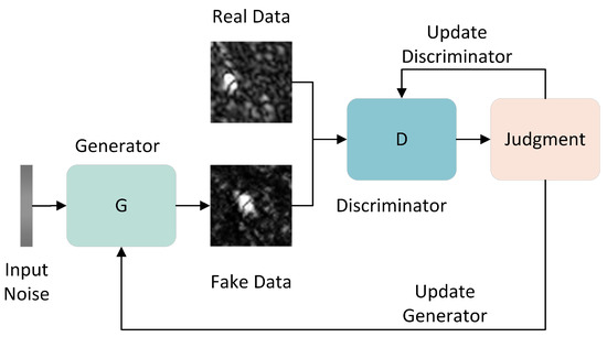
Figure 5.
GAN process.
Since the vanilla GAN was proposed, many works [25,28,29] successively improved it and proposed various variants, where DCGAN [28] and LSGAN [25] are the more well-known GAN variants. The vanilla GAN network tends to gradient disappears because the JS divergence is used to measure the distance between two distributions. The Jensen-Shannon (JS) divergence is constant if there is no intersection between two distributions. In practice, there is a negligible probability of an intersection between the data distribution generated by the generator and the real data distribution. Consequently, the discriminator can easily identify the difference, resulting in the disappearance of the gradient. LSGAN weakens the discriminator to solve this problem by changing the sigmoid activation layer in the discriminator to a linear activation layer. Although the two distributions do not intersect, the difference between the two distributions cannot be distinguished, solving the problem of vanishing gradients.
DCGAN is another variant based on GAN, consistent with GAN in principle. Given the successful application of CNNs in image recognition, DCGAN replaces the multilayer-perceptual network of the generator and discriminator with the convolutional network. Although GAN’s exquisite network structure design enables it to complete self-supervised learning data distribution, the network’s training is unstable, leading to some meaningless results. DCGAN is based on convolutional networks, and the details of the network structure are adjusted to speed up the network convergence and improve the quality of the samples. These detailed structural adjustments include adding data normalization in the generator and discriminator networks, using the tanh activation function in the last layer of the G network, and using the rectified linear unit (ReLU) activation function in the other layers LeakyReLU as the activation function in the D network function.
Previous studies have proposed different evaluation metrics to evaluate the GAN models. Inception score (IS) and Fréchet inception score (FID) [30] are two widely used evaluation indicators. IS is used to assess the generated images based on the JS divergence of the two distributions, while FID is based on the mean and variance of the data distributions. IS evaluates the GAN networks from two perspectives: generated image quality and diversity. The higher the quality of the generated image, the smaller the conditional entropy. The larger the edge probability entropy, the more diverse the generated images.
The performance indicators of IS are expressed as the Kullback-Leibler (KL) divergence, where the larger KL divergence indicates the higher diversity and quality of the generated images. FID is based on the inception net network, which obtains a 2048-dimensional feature. The principle of FID is that the generated data distribution should be as similar as possible to the real data distribution. The mean and covariance are used to calculate the distance between the two distributions. The IS and FID formulas are as follows:
where is the data distribution of the generated image, is the image sampled by x from , is the KL divergence of the distributions p and q, is the distribution of the label y under the condition of x, and is the distribution of the label y.
where is the distribution mean of the real data, is the distribution mean of the generated data, is the distribution variance of the real data, is the variance of the generated data, and is the trace of the matrix. The lower the value of FID, the closer the two distributions and the higher quality and diversity of the generated images. Therefore, this study combines the IS and FID scores to evaluate the images generated by different GANs. The results in Section 4.1 demonstrate that the foliage-penetrating SAR images obtained by the DCGAN network have larger IS and smaller FID scores.
3.5. CARABAS-II Dataset
In remote sensing, the absence of labeled data impedes training a deep network, notably in synthetic aperture radar (SAR) image interpretation, compared to the large-scale annotated dataset in natural photographs.
Large datasets can significantly increase the accuracy and stability of deep learning networks, but they are not often available because of the cost of collection and the difficulty of labeling. SAR images, especially foliage-penetrating SAR images, are difficult to obtain. To our knowledge, CARABAS-II [31] is the only open-source foliage-penetrating SAR image dataset, with just 24 images. To improve the reliability of AMS-CNN, we utilize the CARABAS-II dataset and data augmentation based on it using DCGAN.
The CARABAS-II dataset [31], which comprises 24 VHF band SAR images obtained during a flight in northern Sweden, was utilized. The SAR system uses HH-polarized radio waves with a transmission frequency of 20–90 MHz and obtains images with a resolution of 2.5 × 2.5 m. The dataset was obtained by four deployments during the flight, including Sigismund, Karl, Fredrik, and Adolf–Fredrik, with the imaged area encompassing 25 military vehicles concealed in the forest. Three types of military vehicles were in the imaged area: TGB11, TGB30, and TGB40; their SAR and natural images are depicted in Figure 1.
The parameters that change in gathered data include incidence angle, flight heading, radio frequency interference (RFI), forest location, and target heading, as shown in Table 1. There are 12 different settings, each repeated, resulting in 24 images. Each captured image covers an area of size 2 × 3 km, containing 10 TGB11s with dimensions 4.4 × 1.9 × 2.2 m, 8 TGB30s with dimensions 6.8 × 2.5 3.0 m, and 7 TGB40s with dimensions 7.8 × 2.5 × 3.0 m. Each pixel size is 1 × 1 m, making the image data have 3000 rows and 2000 columns, and the distance between two vehicles is about 50 m. Given that the extracted images only include one type of vehicle, we obtained SAR images of each vehicle with a size of 38 × 38, corresponding to the setting in [5].

Table 1.
Oprating conditions in the CARABAS-II dataset.
4. Results
In this section, we experiment with multiple GAN variants to generate synthetic SAR images, and the visualized and quantitative results are reported. More importantly, we evaluate the performance of AMS-CNN on the foliage-penetrating SAR dataset that is shown in Table 3. Specifically, we discuss them from three different aspects: comparative, ablation, and robustness. The experimental software platform was Pytorch 1.11.0, widely used in deep learning platforms. The GPU used was NVIDIA RTX A2000. In our experiment, the learning rate was set as 0.0001.
4.1. GAN Selection
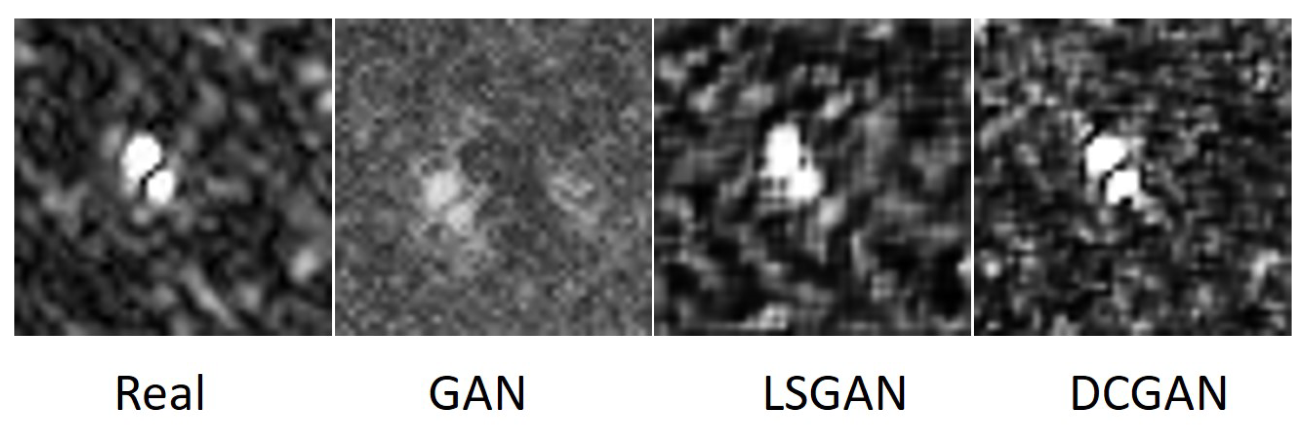
All data in the dataset except the test set is used as training data for GANs. The GAN, LSGAN, and DCGAN visualization results are shown in Figure 6, where the synthetic TGB11 images obtained by different GANs are presented. Compared with the real image obtained by SAR, the synthetic SAR image generated by vanilla GAN looks blurry visually, where the basic outline of the TGB11 vehicle images exists, but the internal details are absent. Moreover, the synthetic SAR images generated by DCGAN and LSGAN are complete regarding outline and interior information. However, the SAR images generated by DCGAN have a clearer outline than LSGAN. Additionally, we adopt IS and FID to quantitatively analyze the results of synthetic SAR images generated by GAN, LSGAN, and DCGAN, shown in Table 2. The quantitative results demonstrate that the DCGAN has the highest IS and lowest FID, consistent with the visualized results. Therefore, the synthetic SAR data generated by DCGAN is used as training samples in this study for DCGAN outperforms the other two networks.
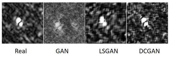
Figure 6.
Synthetic TGB11 SAR images of each GAN.

Table 2.
IS and FID score of each GAN.
We choose the same amount of each vehicle in the real data to guarantee the balance of the different vehicles in the dataset. TGB40 has the least data, so TGB11 and TGB30 choose the same amount as TGB40, resulting in a total dataset of 504 and 168 samples per class. We selected 396 samples for training and 108 samples for testing. DCGAN performs an equal amount of data augmentation for each vehicle category in the dataset, leading to 393 synthetic SAR images. Therefore, the dataset we utilized for foliage-penetrating SAR image classification has 897 samples, and the sample size for training and testing is provided in Table 3, using the same settings as the previous study [5].

Table 3.
The sample size of real and synthetic data in the dataset.
4.2. Comparative Experiments of AMS-CNN
To demonstrate the effectiveness of our proposed model, we compare the foliage-penetrating SAR image classification accuracy of AMS-CNN to that of a recently relevant network, which is shown in Table 4. Simultaneously, we give the parameters of two models in Table 4. On top of the previous work on the foliage-penetrating SAR image classification, we also compared our model with the classical CNNs, like AlexNet [27], VGG16 [32], and GoogleNet [33]. AlexNet is the first work to adopt CNN for classification, which achieves higher accuracy than the traditional machine learning methods. Therefore, it attracted much attention when released and became the milestone of deep learning. To improve the performance of CNN, VGG16 has a deep network with 16 layers to extract the high-level features. Simultaneously, GoogleNet increases not only the deep but also the width to improve its performance. As for the classical CNNs, we adopt the same parameters setting with the AMS-CNN and conduct the experiments.

Table 4.
Accuracy and the number of parameters of different models.
As depicted in Table 4, AMS-CNN outperforms the other networks, where the classification accuracy is 96.8%. In the classical CNNs, the VGG16 achieves the highest accuracy, whereas the GoogleNet performs the worst. It demonstrates that the deep networks adopting the low-resolution SAR images training dataset are more effective than the width networks when CNN only focuses on deep and width. ROC-VGG [5] based on the VGG11 is a pioneer using CNN for foliage-penetrating SAR image classification, which yields higher accuracy than traditional machine learning methods. Compared with the classical CNNs, ROC-VGG performs better, where the classification accuracy is slightly higher than VGG16, indicating the VOC can effectively improve the accuracy. Unlike ROC-VGG, which is based on VGG and uses Receiver Operating Characteristic (ROC) to determine ultimate accuracy, our method proposes a novel framework that powers CNN with a multi-stream and attention mechanism. To verify the impact of the attention blocks, we experiment with the AMS-CNN without them, where the classification accuracy is lower than AMS-CNN with attention blocks and even lower than the ROC-VGG. It indicates that the attention mechanism prioritizes significant information, and the multi-stream focus on the different feature extraction, which are critical for useful feature extraction.
Additionally, the number of parameters for all these CNNs is shown in Table 4. VGG16 and GoogleNet have a number of parameters with and , which both have a large number of parameters because these two models that focus on increasing parameters to improve the accuracy. ROC-VGG based on the VGG11 falls into the VGG series and has many parameters. However, our proposed AMS-CNN has fewer parameters than ROC-VGG, which is only , indicating that AMS-CNN is lightweight and easy to deploy to the device. AMS-CNN is lightweight because of the multi-stream and attention modules we built to extract significant and different information, improving classification accuracy and reducing model parameters.
4.3. Ablation Experiment of AMS-CNN
In addition to the comparative experiments between the proposed AMS-CNN and previous work for foliage-penetrating SAR image classification, we investigate ablation experiments of AMS-CNN from two aspects: model parameters and structure. Specifically, we experiment with batch size, iteration, and regularization hyperparameters, which significantly affect the model performance. We study the different parameter settings. Moreover, the ability of the models to extract features varies depending on the model structures, where we focus on the attention blocks and multiple streams. We set the different spatial and channel attention positions to obtain the performance on the foliage-penetrating SAR images. ASM-CNN adopts three streams: maximum, average, and media. However, the effectiveness of each stream and the combination of the two of them is still unknown to us. Therefore, we also investigate these settings of streams to the model performance.
Model parameters. The study [34] indicates efficient use of vast batch sizes can significantly reduce the model parameters update and improve the performance. The larger the batch size, the more accurate the descending direction, and the smaller the vibration. Simultaneously, [35] has demonstrated that the quality of CNN models degrade for generation performance when they adopt the larger batch size of the parameter using the stochastic gradient descent (SGD) and its variants to update the model. More specifically, the large batch size of the CNN models tends to convert to sharp minima, which greatly impacts generalization performance, while the small batch size has been prone to flatten minima. The number of model parameter updates is affected by the number of iterations. The value of the loss function decreases as the number of updates of the model parameters increases, but there is a risk of model overfitting. According to the introduction of neural networks and deep learning [36], CNN models tend to overfit when the dataset is limited, where the model performs higher accuracy in the training data while the lower accuracy in the testing data. Given the dataset in our experiment is limited, we conduct the L2 regularization to reduce the overfitting, where L2 regularization can reduce the value of the model parameters to decrease network complexity. As such, we explore the impact of batch size, iterations, and regularization parameters on the model.
Table 5 shows the results of our investigation into classification accuracy based on batch size and iterations. We experiment with the batch size setting in 16, 32, and 48, respectively. We further obtain classification accuracy using these three different batch sizes, and the findings show that 32 is the best batch size, and the accuracy worsens when the batch size grows or decreases. Five different iteration settings were explored, such as 400, 800, 1200, 1600, and 2000, with iteration 1600 achieving the highest accuracy. Simultaneously, we experiment with the regularization parameters of four different settings, which are set to 0, 0.1, 0.5, and 1. The regularization parameter in the model significantly reduces model overfitting, with the model performing better when the is set to 0.5, shown in Table 6. Therefore, we adopt a value of 0.5 for the regularization parameter in the experiment.

Table 5.
Recognition accuracy of different iterations and batch sizes.

Table 6.
Recognition accuracy of different regularization parameters .
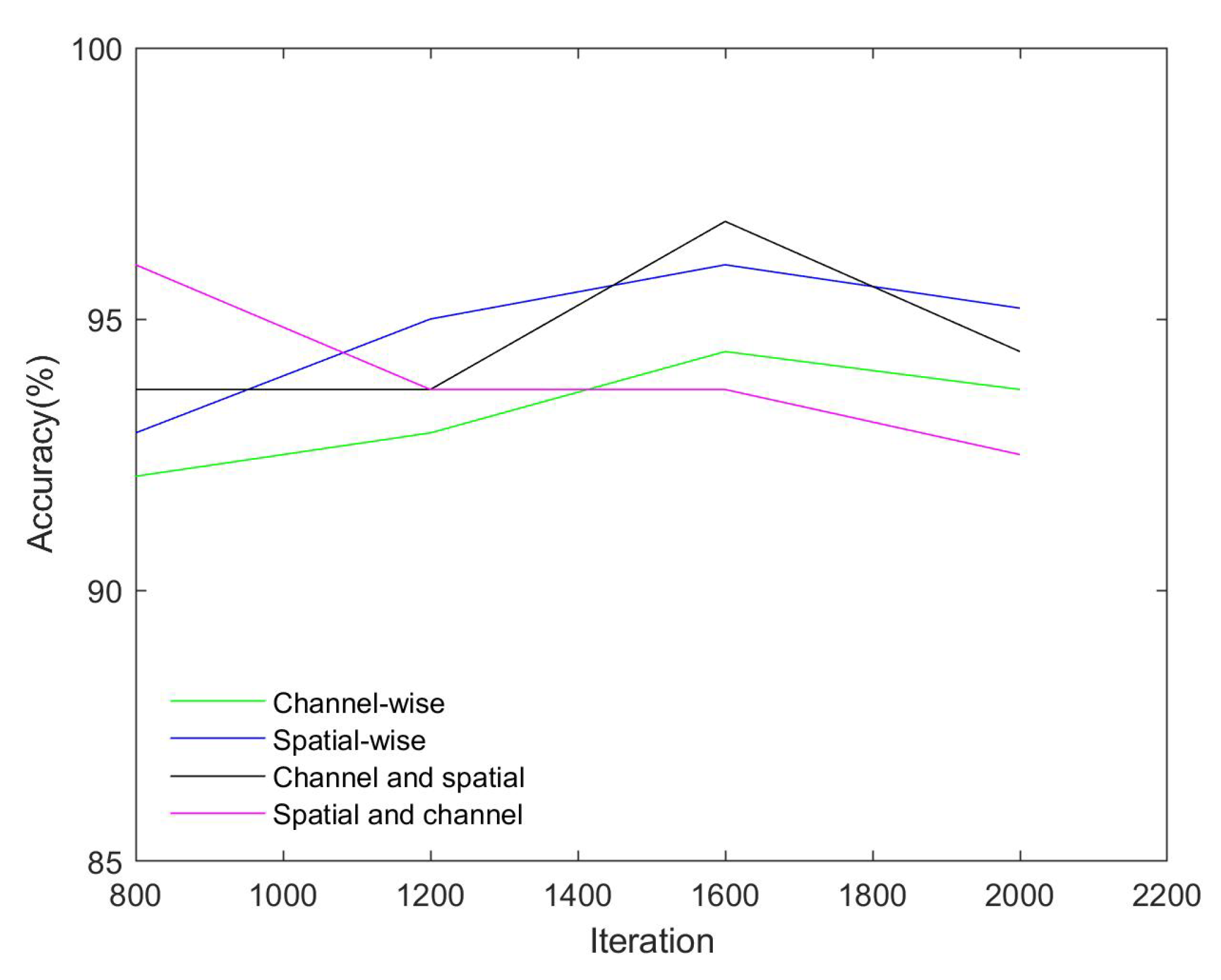
Attention block. The attention blocks, where the spatial, channel, and mixed of them are always employed in SAR image classification, are a key design of our AMS-CNN. We adopt attention blocks after the first two convolutional blocks in AMS-CNN and compare the performance of AMS-CNN based on different attention domains, depicted in Table 7. This experiment uses four configurations: channel-wise, spatial-wise, channel and spatial, and spatial and channel. The first two indicate that the attention domain of two locations in AMS-CNN is the same whether channel or spatial attention is used. The configuration channel and spatial indicate that the first location is the channel attention module, the second is the spatial attention module, and the configuration spatial and channel are the inverse. We also explore the classification accuracy of four attention settings on the different iterations.

Table 7.
The recognition accuracy of different attention domains configuration.
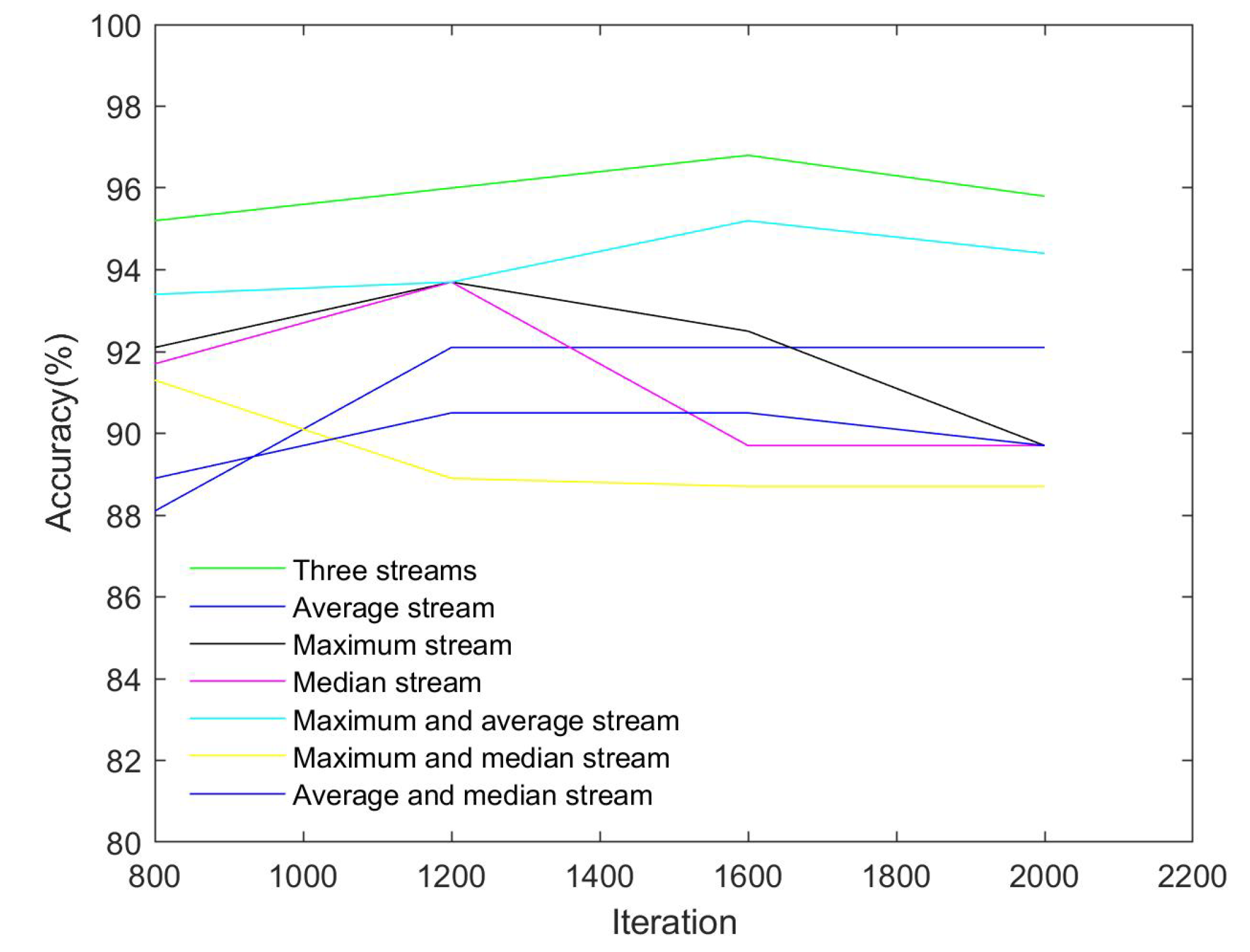
Multi-stream structures. Three streams are used in our work: average, maximum, and median streams. The possible combinations of the three streams are explored, including seven settings: three one-stream, two-stream, and one three-stream (the default setting). Table 8 shows the influence of different steam settings on foliage-penetrating SAR images accuracy. The maximum stream outperforms the other two one-stream models with a classification accuracy of 92.5 % in the optimal iteration setting of 1600, indicating the maximum stream can extract important features beneficial for the classification. The two-stream model with maximum and average stream performs better, while the two-stream model with maximum and median stream performs worst in the default iteration number of 1600. The two-stream model with maximum and average streams performs better than the one-stream maximum and average models, which indicates the maximum stream and the average stream can promote each other to extract features for classification. However, the two-stream models with one of the streams as the median stream, performs worse than the one-stream model with the maximum or average stream.

Table 8.
Recognition accuracy of different streams setting.
4.4. Robustness Experiment of AMS-CNN
Deep learning models are widely considered to dominate the field of computer vision in recent years, which achieve remarkable performance on many standard benchmarks. Unlike human vision, which is robust to the situation that the distribution of train and test data differ, the deep learning models lack robustness to this [37]. For example, the input test images with some forms of corruption (e.g., uniform noise, Gaussian noise ) tend to mislead the models, resulting in misleading classification.
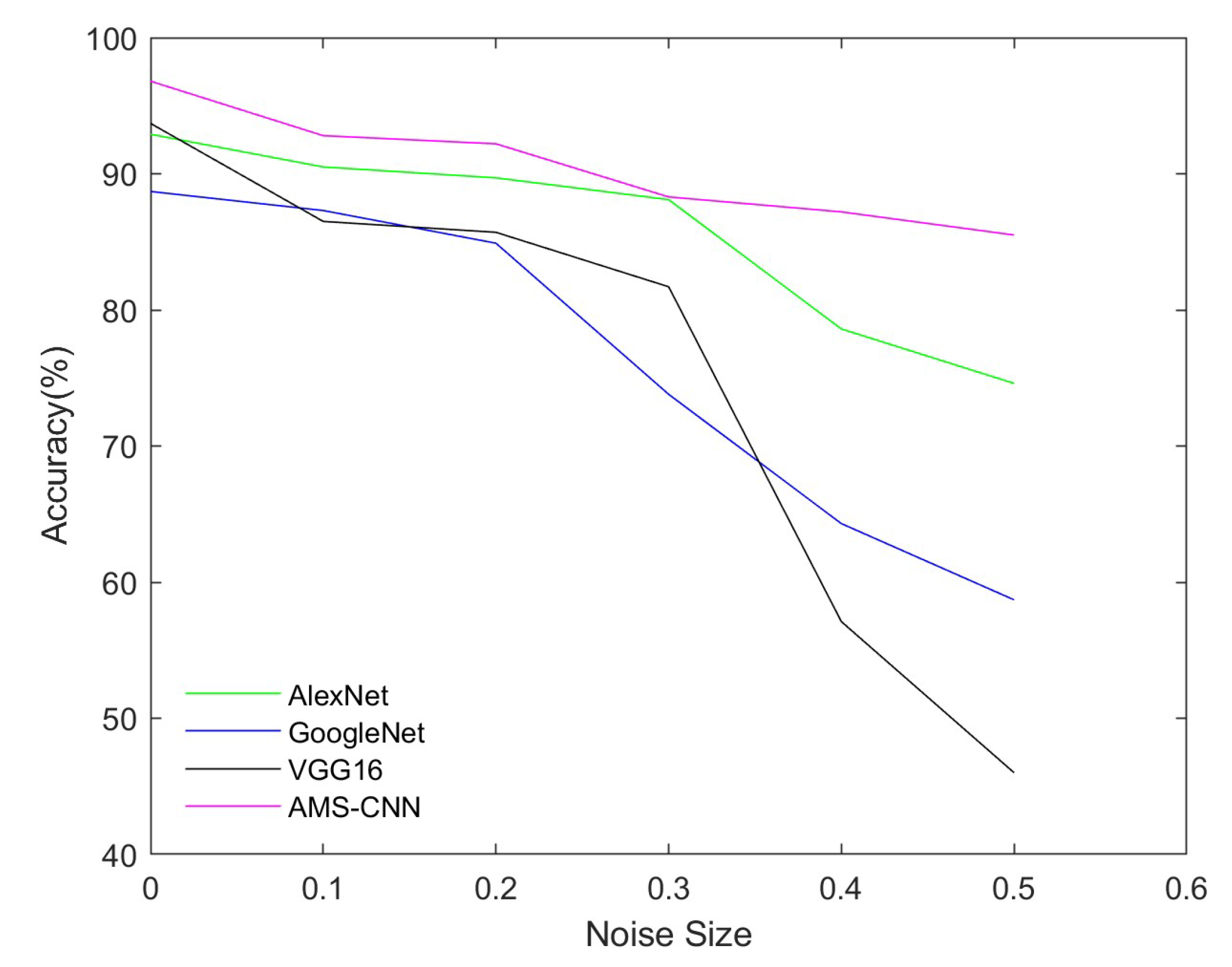
To evaluate the robustness of our proposed AMS-CNN, uniform noise with five different severity is adopted to the test foliage-penetrating SAR images. Simultaneously, the three classical CNN models, including AlexNet, GoogleNet, and VGG16, are also evaluated for the robustness with the distribution of test data that differs from the train data, where the test data is added by the uniform noise. We investigate its accuracy performance when noise is added to test samples and compare it to the other three classical models under the same conditions. In this experiment, we compare our proposed method with three classic CNNs based on the same hyperparameter settings, and random uniform noise of various sizes is added to test images. Table 9 gives different models’ classification accuracy.

Table 9.
Evaluation results on images with added noise.
5. Discussion
On the different attention block settings of AMS-CNN. The classification accuracy of different attention settings is illustrated in Figure 7. The model’s performance with spatial and channel attention rapidly deteriorates as iterations increase from 1200 to 1600. Unlike the model with spatial and channel attention, the model with the other three settings improves gradually, with iteration 1600 yielding the best accuracy. The optimal configuration, the first convolutional block followed by channel attention and the second convolutional block followed by spatial attention, achieves 96.8% classification accuracy, while the configuration spatial and channel performs the worst. Given this condition, one plausible explanation is that we should prioritize channel attention for low-level characteristics while prioritizing spatial attention for high-level features.
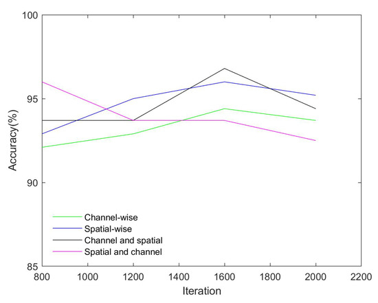
Figure 7.
Evaluation of the different attention settings.
On the different streams of AMS-CNN. We explore the effect of varied steams on classification accuracy with different iteration settings, as shown in Figure 8, where we use one-stream and two-stream models for the classification. As the number of iterations increases to 1200, the classification recognition accuracy of the one-stream model increases. Moreover, the two-stream models perform differently from the one-stream models. When the number of iterations increases to 1600, the accuracy of AMS-CNN with the default hyperparameter setting (iteration of 1600) increases, whereas the accuracy of the other three models based on a one-stream decreases. The classification accuracy of the network with one stream is worse than that of three streams, where the latter provides adequate information for SAR image information. Simultaneously, the network with one different stream performs differently, whereas the network with maximum stream outperforms others. The capacity of the three streams of AMS-CNN to extract information may differ, with merging the three streams yielding the essential features.
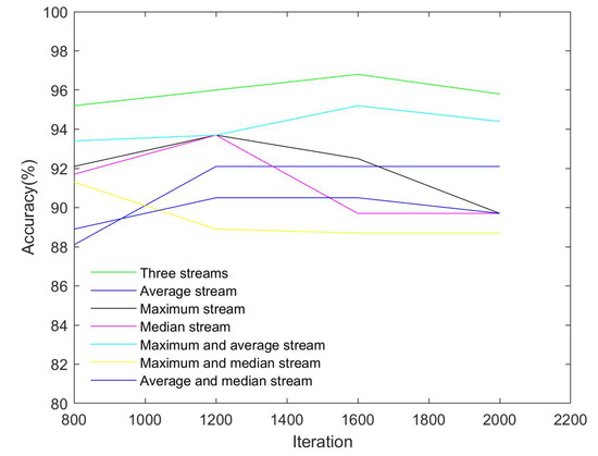
Figure 8.
Evaluation of the different stream settings (the proposed AMS-CNN with three steams).
On the robustness of AMS-CNN. The robustness of different CNN models is analyzed, where we adopt test set images with five different sizes of random uniform noise. Figure 9 depicts the effects of varying noise sizes on the classification accuracy of different CNN models. The finding shows that the classification accuracy decreases as the noise size increases. However, as the noise size increases, the accuracy of the four models decreases to varying degrees, with AMS-CNN dropping the least and Vgg16 dropping the most. Vgg16 performs less robustness, although it has better image classification accuracy in clean images for its deep network structure. Simultaneously, AMS-CNN has better image classification accuracy in clean and noisy images. The reason is that our AMS-CNN is designed to extract key and multiple features for image classification, making it more robust to images with added noise.
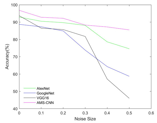
Figure 9.
Evaluation of the noised images for different models.
6. Conclusions
A lightweight AMS-CNN boosted by attention modules and multi-stream heads is proposed in this paper, which extends the success of lightweight CNN used in natural images to low-resolution SAR images. Specifically, in our proposed method, the attention modules based on channel and spatial domains are utilized to automatically select important low-level features, while the multi-stream heads focus on gathering diverse high-level features. Moreover, DCGAN is utilized to address the limited foliage-penetrating SAR dataset. Different attention domains and stream settings are compared, as well as various iterations and batch sizes. To validate the performance of AMS-CNN, we compared it to the previous model ROC–VGG, and the results showed that AMS-CNN performs well with fewer parameters. Moreover, different noise sizes were used to test the robustness of AMS-CNN, and a comparison of the accuracy of different models shows that AMS-CNN was more robust. Overall, our proposed lightweight method is simple, effective, and robust, constituting a strong baseline for future works to study SAR classification.
Author Contributions
Conceptualization, S.Z. and X.H.; methodology, S.Z. and C.Z.; software, S.Z. and W.Z.; validation, S.Z. and X.H; formal analysis, S.Z. and C.Z.; investigation, L.D.; resources, S.Z.; data curation, W.Z.; writing—original draft preparation, S.Z. and C.Z..; writing—review and editing, S.Z. and C.Z.; visualization, W.Z.; supervision, X.H.; project administration, X.H.; funding acquisition, X.H. All authors have read and agreed to the published version of the manuscript.
Funding
This research was funded by the National Natural Science Foundation of China, grant number 61871414, and partly by the Basic Strengthening Project of Military Science and Technology Commission 2019-JCJQ-ZD-324.
Data Availability Statement
The research data is available in https://www.sdms.afrl.af.mil/index.php?collection=mstar&page=targets (accessed on 9 May 2023).
Acknowledgments
We thank the National Natural Science Foundation of China and the Military Science and Technology Commission for their financial support. We would also like to thank the handling Associate Editor and the anonymous reviewers for their valuable comments and suggestions for this paper.
Conflicts of Interest
The authors declare no conflict of interest.
Abbreviations
The following abbreviations are used in this manuscript:
| SAR | Synthetic aperture radar |
| AMS-CNN | Attention-based multi-stream convolutional neural network |
| SOC | Standard Operating Conditions |
| EOC | Extended Operating Conditions |
| GAN | Generative adversarial network |
| SVM | Support vector machine |
| AdaBoost | Adaptive boosting |
| RBF | Radial basis function |
| CNN | Convolutional neural network |
| DCGAN | Deep convolutional generative adversarial network |
| MGAN | Multi-discriminator generative adversarial network |
| CN-GAN | Constrained naive generative adversarial network |
| LSGAN | Least Squares generative adversarial network |
| Pix2Pix | Image-to-image transation |
| JS | Jensen–Shannon |
| ReLU | Rectified linear unit |
| IS | Inception score |
| FID | Fréchet inception score |
| RFI | Radio frequency interference |
| ROC | Receiver Operating Characteristic |
References
- Lu, J. Design Technology of Synthetic Aperture Radar; John Wiley & Sons: Hoboken, NJ, USA, 2019. [Google Scholar]
- Chen, J.; Xing, M.; Yu, H.; Liang, B.; Peng, J.; Sun, G.C. Motion compensation/autofocus in airborne synthetic aperture radar: A review. IEEE Geosci. Remote Sens. Mag. 2021, 10, 185–206. [Google Scholar] [CrossRef]
- Zhang, X.; Wu, H.; Sun, H.; Ying, W. Multireceiver SAS imagery based on monostatic conversion. IEEE J. Sel. Top. Appl. Earth Obs. Remote Sens. 2021, 14, 10835–10853. [Google Scholar] [CrossRef]
- Choi, H.m.; Yang, H.s.; Seong, W.j. Compressive underwater sonar imaging with synthetic aperture processing. Remote Sens. 2021, 13, 1924. [Google Scholar] [CrossRef]
- Vint, D.; Anderson, M.; Yang, Y.; Ilioudis, C.; Di Caterina, G.; Clemente, C. Automatic target recognition for low resolution foliage penetrating SAR images using CNNs and GANs. Remote Sens. 2021, 13, 596. [Google Scholar] [CrossRef]
- He, K.; Zhang, X.; Ren, S.; Sun, J. Deep residual learning for image recognition. In Proceedings of the IEEE Conference on Computer Vision and Pattern Recognition, Las Vegas, NV, USA, 27–30 June 2016; pp. 770–778. [Google Scholar]
- Zagoruyko, S.; Komodakis, N. Wide residual networks. arXiv 2016, arXiv:1605.07146. [Google Scholar]
- Hu, J.; Shen, L.; Sun, G. Squeeze-and-excitation networks. In Proceedings of the IEEE Conference on Computer Vision and Pattern Recognition, Salt Lake City, UT, USA, 18–23 June 2018; pp. 7132–7141. [Google Scholar]
- Woo, S.; Park, J.; Lee, J.Y.; Kweon, I.S. Cbam: Convolutional block attention module. In Proceedings of the European Conference on Computer Vision (ECCV), V), Munich, Germany, 8–14 September 2018; pp. 3–19. [Google Scholar]
- Hu, Y.; Lu, M.; Lu, X. Driving behaviour recognition from still images by using multi-stream fusion CNN. Mach. Vis. Appl. 2019, 30, 851–865. [Google Scholar] [CrossRef]
- Chen, D.; Zhang, S.; Ouyang, W.; Yang, J.; Tai, Y. Person search via a mask-guided two-stream cnn model. In Proceedings of the European Conference on Computer Vision (ECCV), Munich, Germany, 8–14 September 2018; pp. 734–750. [Google Scholar]
- Li, R.; Wang, X.; Wang, J.; Song, Y.; Lei, L. SAR target recognition based on efficient fully convolutional attention block CNN. IEEE Geosci. Remote Sens. Lett. 2020, 19, 1–5. [Google Scholar] [CrossRef]
- Shi, B.; Zhang, Q.; Wang, D.; Li, Y. Synthetic aperture radar SAR image target recognition algorithm based on attention mechanism. IEEE Access 2021, 9, 140512–140524. [Google Scholar] [CrossRef]
- Wang, D.; Song, Y.; Huang, J.; An, D.; Chen, L. SAR Target Classification Based on Multiscale Attention Super-Class Network. IEEE J. Sel. Top. Appl. Earth Obs. Remote Sens. 2022, 15, 9004–9019. [Google Scholar] [CrossRef]
- Zhang, M.; An, J.; Yang, L.D.; Wu, L.; Lu, X.Q. Convolutional neural network with attention mechanism for SAR automatic target recognition. IEEE Geosci. Remote Sens. Lett. 2020, 19, 1–5. [Google Scholar]
- Chen, S.; Wang, H.; Xu, F.; Jin, Y.Q. Target classification using the deep convolutional networks for SAR images. IEEE Trans. Geosci. Remote Sens. 2016, 54, 4806–4817. [Google Scholar] [CrossRef]
- Zhao, P.; Liu, K.; Zou, H.; Zhen, X. Multi-stream convolutional neural network for SAR automatic target recognition. Remote Sens. 2018, 10, 1473. [Google Scholar] [CrossRef]
- Huang, X.; Yang, Q.; Qiao, H. Lightweight two-stream convolutional neural network for SAR target recognition. IEEE Geosci. Remote Sens. Lett. 2020, 18, 667–671. [Google Scholar] [CrossRef]
- Zeng, Z.; Sun, J.; Han, Z.; Hong, W. SAR automatic target recognition method based on multi-stream complex-valued networks. IEEE Trans. Geosci. Remote Sens. 2022, 60, 1–18. [Google Scholar] [CrossRef]
- Goodfellow, I.; Pouget-Abadie, J.; Mirza, M.; Xu, B.; Warde-Farley, D.; Ozair, S.; Courville, A.; Bengio, Y. Generative adversarial networks. Commun. ACM 2020, 63, 139–144. [Google Scholar] [CrossRef]
- Gao, F.; Liu, Q.; Sun, J.; Hussain, A.; Zhou, H. Integrated GANs: Semi-supervised SAR target recognition. IEEE Access 2019, 7, 113999–114013. [Google Scholar] [CrossRef]
- Du, S.; Hong, J.; Wang, Y.; Qi, Y. A high-quality multicategory SAR images generation method with multiconstraint GAN for ATR. IEEE Geosci. Remote Sens. Lett. 2021, 19, 1–5. [Google Scholar] [CrossRef]
- Zheng, C.; Jiang, X.; Liu, X. Semi-supervised SAR ATR via multi-discriminator generative adversarial network. IEEE Sensors J. 2019, 19, 7525–7533. [Google Scholar] [CrossRef]
- Mao, C.; Huang, L.; Xiao, Y.; He, F.; Liu, Y. Target recognition of SAR image based on CN-GAN and CNN in complex environment. IEEE Access 2021, 9, 39608–39617. [Google Scholar] [CrossRef]
- Mao, X.; Li, Q.; Xie, H.; Lau, R.Y.; Wang, Z.; Paul Smolley, S. Least squares generative adversarial networks. In Proceedings of the IEEE International Conference on Computer Vision, Venice, Italy, 22–29 October 2017; pp. 2794–2802. [Google Scholar]
- Isola, P.; Zhu, J.Y.; Zhou, T.; Efros, A.A. Image-to-image translation with conditional adversarial networks. In Proceedings of the IEEE Conference on Computer Vision and Pattern Recognition, Honolulu, HI, USA, 21–26 July 2017; pp. 1125–1134. [Google Scholar]
- Krizhevsky, A.; Sutskever, I.; Hinton, G.E. Imagenet classification with deep convolutional neural networks. Commun. ACM 2017, 60, 84–90. [Google Scholar] [CrossRef]
- Radford, A.; Metz, L.; Chintala, S. Unsupervised representation learning with deep convolutional generative adversarial networks. arXiv 2015, arXiv:1511.06434. [Google Scholar]
- Brock, A.; Donahue, J.; Simonyan, K. Large scale GAN training for high fidelity natural image synthesis. arXiv 2018, arXiv:1809.11096. [Google Scholar]
- Heusel, M.; Ramsauer, H.; Unterthiner, T.; Nessler, B.; Hochreiter, S. Gans trained by a two time-scale update rule converge to a local nash equilibrium. In Proceedings of the 31st International Conference on Neural Information Processing Systems, Long Beach, CA, USA, 4 December 2017; Volume 30. [Google Scholar]
- Lundberg, M.; Ulander, L.M.; Pierson, W.E.; Gustavsson, A. A challenge problem for detection of targets in foliage. In Proceedings of the Algorithms for Synthetic Aperture Radar Imagery XIII, Kissimmee, FL, USA, 17–20 April 2006; SPIE: Bellingham, WA, USA, 2006; Volume 6237, pp. 160–171. [Google Scholar]
- Simonyan, K.; Zisserman, A. Very deep convolutional networks for large-scale image recognition. arXiv 2014, arXiv:1409.1556. [Google Scholar]
- Szegedy, C.; Liu, W.; Jia, Y.; Sermanet, P.; Reed, S.; Anguelov, D.; Erhan, D.; Vanhoucke, V.; Rabinovich, A. Going deeper with convolutions. In Proceedings of the IEEE Conference on Computer Vision and Pattern Recognition, Boston, MA, USA, 7–12 June 2015; pp. 1–9. [Google Scholar]
- Smith, S.L.; Kindermans, P.J.; Ying, C.; Le, Q.V. Don’t decay the learning rate, increase the batch size. arXiv 2017, arXiv:1711.00489. [Google Scholar]
- Keskar, N.S.; Mudigere, D.; Nocedal, J.; Smelyanskiy, M.; Tang, P.T.P. On large-batch training for deep learning: Generalization gap and sharp minima. arXiv 2016, arXiv:1609.04836. [Google Scholar]
- Nielsen, M.A. Neural Networks and Deep Learning; Determination Press: San Francisco, CA, USA, 2015; Volume 25. [Google Scholar]
- Recht, B.; Roelofs, R.; Schmidt, L.; Shankar, V. Do imagenet classifiers generalize to imagenet? In Proceedings of the International Conference on Machine Learning, Long Beach, CA, USA, 9–15 June 2019; pp. 5389–5400. [Google Scholar]
Disclaimer/Publisher’s Note: The statements, opinions and data contained in all publications are solely those of the individual author(s) and contributor(s) and not of MDPI and/or the editor(s). MDPI and/or the editor(s) disclaim responsibility for any injury to people or property resulting from any ideas, methods, instructions or products referred to in the content. |
© 2023 by the authors. Licensee MDPI, Basel, Switzerland. This article is an open access article distributed under the terms and conditions of the Creative Commons Attribution (CC BY) license (https://creativecommons.org/licenses/by/4.0/).


