Application of a Modified BP_S Neural Network Based on Three-Way Decision Theory in an Effectiveness Evaluation for a Remote Sensing Satellite Cluster

Abstract

The remote sensing satellite cluster system, as an important component of the next generation of space architecture in the United States, has important application prospects in the military field. In order to improve the effects of time, with regard to the effectiveness evaluation of the remote sensing satellite cluster system, neural network methods are generally used to satisfy the requirements of real-time decision-making assistance in the military field. However, there are two problems that emerge when applying the existing neural network methods to an effectiveness evaluation of the remote sensing satellite cluster. On the one hand, the neural network model architecture needs to be designed specifically for the remote sensing satellite cluster system. On the other hand, there is still a lack of hyperparameter optimization methods that consume less time and have good optimization effects for the established neural network model. In this regard, two main modifications were made to the back-propagation neural network, to which an effectiveness evaluation was applied. The first comprised a new architecture named BP_S, which was designed for the back-propagation neural network so as to improve its prediction accuracy. In BP architecture, one back-propagation neural network is established for each indicator involved in the effectiveness evaluation indicator system of the remote sensing satellite cluster; the output of each back-propagation neural network model is modified to the residual value between the corresponding indicator value and the value that is predicted through a multiple linear regression analysis of the corresponding indicator. The second modification involved the multi-round traversal method, which is based on the three-way decision theory, and it was proposed in order to significantly improve the model’s training time, which is a new type of hyperparameter optimization method. The results show that compared with the traditional simulation model, the modified back-propagation neural network model based on three-way decision theory can quickly and effectively provide stable and accurate evaluation results; this can assist with and meet the requirements for real-time decision-making in the military field.

1. Introduction

The United States released the National Security Space Strategy (NSSS) in 2011. The NSSS mainly focuses on the problem of space confrontation, and it emphasizes “flexibility” as an important indicator with which to evaluate the military space system to ensure the security of its space capabilities [1,2]. After years of research, demonstrations, and tests, the United States released the National Space Strategy in 2018, which focuses on the elastic space system as an important means with which to establish the absolute advantages of space and its ability to act as a nuclear deterrent [3,4,5]. Subsequently, NASA proposed the next generation of space architecture for the first time at the 35th Space Seminar held in April 2019, which includes seven functional layers: the space transmission layer, tracking layer, monitoring layer, deterrence layer, navigation layer, combat management layer, and support layer. As an important part of the next generation of space architecture, the tracking layer and the monitoring layer are mainly used to provide reconnaissance information and early warnings of sea, land, and air targets; this is achieved by equipping electronic reconnaissance, optical imaging, and radar imaging payloads, among others. In light of the abovementioned requirements, the US Department of Defense has planned a project focusing upon a hypersonic and ballistic tracking space sensor, which was initially a large-scale, low-orbit, remote-sensing satellite cluster composed of multiple small sensor satellites [6].

In order to establish a more perfect remote-sensing satellite cluster system, it is essential to evaluate the effectiveness of the remote-sensing satellite cluster. An effectiveness evaluation can start by assessing the needs of remote sensing applications and finding out the weaknesses of the remote sensing satellite cluster system, so as to better optimize the remote sensing satellite cluster system [7]. Moreover, a reasonable and scientific effectiveness evaluation can provide strong support for the demand concerning demonstrations and the system development of remote sensing satellites; it can speed up the development process of remote sensing satellites, optimize the allocation of satellite resources, and improve the operational efficiency of satellites. It is evident that the accurate and effective evaluation of the effectiveness of a remote sensing satellite cluster is of great importance to the design, operation, and maintenance of the constellation configuration, and it is the basis for the optimization of the constellation structure [8].

With the development of complex system simulation technology, computer technology, and data management technology, the granularity of simulation models is getting finer and more complex. The simulation data gradually present characteristics of larger data. In addition, there are prominent problems such as information redundancy and a high correlation among evaluation indicators. It is well known that the higher the accuracy of the model, the more accurate the effectiveness evaluation, and the more consistent it is with the real situation. At present, there are several effectiveness evaluation methods, such as the analytic hierarchy process (AHP) [7,9,10], ADC (availability, dependability, capability) model [11,12,13], fuzzy comprehensive evaluation method [14,15,16,17], grey evaluation method [18], neural network method [8,19], and so on. It is worth noting that all of the abovementioned effectiveness evaluation methods, except the neural network method, have the following two shortcomings. On the one hand, the methods are weak for processing large data. On the other hand, the low efficiency of the simulation calculations of the methods leads to time-consuming effectiveness evaluations, which cannot support the demand of real-time decision-making. In recent years, with the rapid development of neural network technology, neural networks have been applied well in many fields [19,20,21,22,23,24,25,26]. An increasing number of researchers have begun to use neural networks to conduct effectiveness evaluations of satellite clusters. ZHOU Xiao-he et al. [27] constructed the operational effectiveness evaluation model for communication satellites using the GA-BP (Genetic Algorithm-Back Propagation) neural network method, and they validated the model using the data generated during the actual working process of the satellite. Li Z et al. [8] proposed a neural network effectiveness evaluation model for remote-sensing satellites, and the proposed model can generate real-time, high-quality evaluation results. Compared with other traditional effectiveness evaluation methods, the neural network method can effectively solve the abovementioned problems and achieve a rapid and accurate effectiveness evaluation. Liu, J. et al. [24] presented a modified event-triggered command filter backstepping tracking control scheme for a class of uncertain nonlinear systems with an unknown input saturation, based on the adaptive neural network (NN) technique, which can avoid the issue of Zeno behavior when subjected to the designed event-triggering mechanism.

The architecture design of the neural network model varies according to the different problems to be solved. The architecture design of the neural network often determines the overall network performance [28,29,30]. Moreover, the hyperparameters such as the number of hidden layers, the number of nodes per layer, and the type of activation function have a direct impact on the training accuracy and generalization ability of the neural network model, and its importance is self-evident. At present, there are generally three methods to optimize the hyperparameters of the neural network, which are manual parameter adjustment [31], grid optimization [32,33], and intelligent algorithm optimization [34,35,36].

This paper mainly focuses on the design of the neural network effectiveness evaluation model for the remote-sensing satellite cluster system, and the architecture design and the optimization of the design parameters of the model have been found to have problems to be solved. On the one hand, the effectiveness evaluation of a remote-sensing satellite cluster system involves many indicators, and the influencing factors of each indicator are different. Specifically, seven core indicators contained within the effectiveness evaluation indicator system of remote sensing satellite cluster and thirteen influencing factors are considered in this paper. The influencing factors mainly include number of orbits, number of satellites per orbit, orbit altitude, etc., which are described in detail in

Table 1. The orbital parameters of the remote sensing satellite cluster.

Parameter Name	Value
Number of orbits	10
Number of satellites per orbit	10
Orbit altitude (km)	650
Orbital inclination (°)	98
The proportion of wide-band satellites	0.2
The view angle of wide-band satellites (°)	10
The view angle of high-resolution satellites (°)	2
Number of pixels	20,000
Maximum attitude maneuver angle (°)	45
Maximum attitude maneuver angular velocity (°/s)	3
Maximum imaging times per orbit	4
Maximum imaging time per orbit (s)	40
Communication rate (Mbps)	400

. The number of neural network models needs to be determined. In other words, whether to use one neural network model to predict all indicators or one neural network model to predict one indicator is a question worth researching. If only one neural network model is used to predict all indicators, we think that the prediction accuracy of the final effectiveness evaluation will be inaccurate. Hence, it is necessary to obtain a better neural network architecture by comparing prediction accuracy results. It should be noted that the architecture design mentioned above refers to not changing the algorithm logic of the traditional neural network, but only changing the output and number of the neural networks. On the other hand, the commonly used hyperparameter optimization methods are not applicable to the neural network effectiveness evaluation model built for remote sensing satellite clusters, and the main reasons are as follows. The remote-sensing satellite cluster system is a very complex system with a large scale. Manual parameter adjustment depends on expert experience and is easily affected by expert subjectivity, so it is inaccurate and usually time-consuming. The grid optimization generally takes long time consumption, and its calculation amount increases exponentially when multiple hyperparameters are considered. Since the remote-sensing satellite cluster effectiveness evaluation index system involves many indicators and the influencing factors of each indicator are different, it is generally necessary to establish corresponding neural network effectiveness evaluation models for each indicator for training, so the more complex the whole system is, the larger the number of neural network effectiveness evaluation models that need to be trained. Intelligent algorithm optimization has certain uncertainty and depends on a large number of computing resources. The effectiveness evaluation indicator system of remote sensing satellite cluster contains a large number of indicators, which will involve a large number of different neural network models. It will multiply the computational resources required to optimize the hyperparameters. Hence, intelligent algorithm optimization is not suitable for this paper. Hence, according to the neural network effectiveness evaluation model built for the remote sensing satellite cluster system, first of all, it is necessary to design a reasonable architecture of the neural network effectiveness evaluation model with stable and higher prediction accuracy, and secondly, it is urgent to need a new hyperparameter optimization method with less time consumption and better optimization effect.

In view of the above problems, the neural network effectiveness evaluation model is improved in two aspects in this paper. On the one hand, based on the effectiveness evaluation indicator system of remote sensing satellite cluster, a new back propagation (BP) neural network architecture named BP_S architecture is designed, which can effectively improve the prediction accuracy of the model. In BP_S architecture, one BP neural network is established for each indicator involved in the effectiveness evaluation indicator system of the remote-sensing satellite cluster, respectively, in BP_S architecture, which means that the output of the BP neural network is one indicator value rather than all indicator values On the other hand, the multi-round traversal method based on the three-way decision theory is designed in order to solve the problem of the low efficiency in model training, which can obtain the optimal hyperparameter combination in a relatively short period of time.

The contributions of this paper can be summarized as follows.

• We compared the prediction accuracy of one BP neural network predicting one indicator value with that of one BP neural network predicting all indicator values, which validates the effectiveness of the BP_S architecture (Section 3.2).
• The types and the range of values for hyperparameters is large. If we directly traverse all hyperparameter combinations to find the optimal one, it will consume a lot of model training time. Hence the multi-round traversal method based on the three-way decision theory is proposed to solve the problem, which can significantly shorten model training time (Section 3.3).

2. The Effectiveness Evaluation Indicator System of Remote Sensing Satellite Cluster

The effectiveness evaluation indicator system of the remote-sensing satellite cluster for moving targets built by reference [8] in this paper is divided into three layers, as shown in Figure 1. Three capabilities are mainly considered in system construction: discovery, identification and confirmation, and continuous tracking.

It can be seen in Figure 1 that the effectiveness evaluation indicator system of remote sensing satellite cluster for moving targets mainly includes six indicators, which are target discovery probability, discovery response time, target identification probability, identification response time, tracking time percentage, average tracking interval, and minimum tracking interval, respectively. The mathematical description and calculation formula of all indicators are given as follows.

The target discovery probability $P_{\mathrm{TD}}$ is defined as the proportion of the number of successfully discovered targets to the total number of targets within a period of time.

$$P_{\mathrm{TD}}=\frac{N_{\mathrm{TD}}}{N_{\mathrm{T}}}$$

(1)

where $N_{\mathrm{TD}}$ is the number of targets discovered successfully within a period of time, and $N_{\mathrm{T}}$ is the total number of targets.

The discovery response time $T_{\mathrm{DR}}$ is calculated by the time from the satellite receiving the discovery mission order to the successful discovery of the target, which is the average value.

$$T_{\mathrm{DR}}=\frac{{\displaystyle \sum _{i=1}^{N_{\mathrm{DM}}}(t_{\mathrm{DMEnd}}^i-t_{\mathrm{DMStart}}^i)}}{N_{\mathrm{DM}}}$$

(2)

where $t_{\mathrm{DMStart}}^i$ is the start time of the i-th successful discovery mission, and $t_{\mathrm{DMEnd}}^i$ is the end time of the i-th successful discovery mission. It should be noted that the start time is defined as the order upload time of one successful discovery mission and the end time is defined as the time when the satellite completes the observation of the target. $N_{\mathrm{DM}}$ is the number of successful discovery mission within a period time.

The target identification probability $P_{\mathrm{TI}}$ is defined as the proportion of the number of targets successfully identified at least once to the number of targets required by at least one identification mission within a period time.

$$P_{\mathrm{TI}}=\frac{N_{\mathrm{TI}}}{N_{\mathrm{TIR}}}$$

(3)

where $N_{\mathrm{TI}}$ is the number of targets successfully identified at least once within a period time, and $N_{\mathrm{TIR}}$ is the number of targets required by at least one identification mission within a period time.

The identification response time $T_{\mathrm{IR}}$ is calculated by the time from the moment the satellite receives the identification mission order to the time it successfully identifies the target, which is the average value. It should be noted that failed identification missions are not counted.

$$T_{\mathrm{IR}}=\frac{{\displaystyle \sum _{i=1}^{N_{\mathrm{RM}}}(t_{\mathrm{RMEnd}}^i-t_{\mathrm{RMStart}}^i)}}{N_{\mathrm{RM}}}$$

(4)

where $N_{\mathrm{RM}}$ is the number of the successful identification missions within a period time. $t_{\mathrm{RMStart}}^i$ and $t_{\mathrm{RMEnd}}^i$ are the start time and end time of the i-th successful identification mission, respectively. It should be noted that the start time is defined as the order upload time of one successful identification mission and the end time is defined as the time when the satellite completes the observation of the target.

The tracking time percentage $A_{\mathrm{TT}}$ is defined as the proportion of total target tracking time to total simulation time.

$$A_{\mathrm{TT}}=\frac{{\displaystyle \sum _{i=1}^{N_{\mathrm{T}}}{\displaystyle \sum _{j=1}^{N_i^{\mathrm{Tr}}}(T_{i,j}^{\mathrm{TrEnd}}-T_{i,j}^{\mathrm{TrStart}})}}}{N_{\mathrm{T}}\times T_{\mathrm{T}}}$$

(5)

where $T_{i,j}^{\mathrm{TrStart}}$ and $T_{i,j}^{\mathrm{TrEnd}}$ are the start time and end time of the j-th tracking mission of the i-th target. $T_i^{\mathrm{Tr}}$ is the total tracking number of the i-th target.

The average tracking interval $T_{\mathrm{AT}}$ is calculated by the interval between two consecutive tracking mission, which is the average value.

$$T_{\mathrm{AT}}=\frac{{\displaystyle \sum _{i=1}^{N_{\mathrm{T}}}{\displaystyle \sum _{j=1}^{N_i^{\mathrm{Tr}}-1}(T_{i,j+1}^{\mathrm{TrStart}}-T_{i,j}^{\mathrm{TrEnd}})}}}{{\displaystyle \sum _{i=1}^{N_{\mathrm{T}}}{N}_i^{\mathrm{Tr}}}}$$

(6)

The minimum tracking interval $T_{\mathrm{MT}}$ is calculated by the interval between two consecutive tracking mission, which is the average value, which is the minimum value.

$$T_{\mathrm{AT}}=\underset{i=1}{\overset{N_{\mathrm{T}}}{\min }}(\underset{j=1}{\overset{N_i^{\mathrm{Tr}}-1}{\min }}(T_{i,j+1}^{\mathrm{TrStart}}-T_{i,j}^{\mathrm{TrEnd}}))$$

(7)

3. A New Neural Network Evaluation Model Training Method for a Remote-Sensing Satellite Cluster

The traditional method of effectiveness evaluation is generally to establish a simulation model and then calculate the required indicator values based on the simulation results obtained through simulation, which can be seen in Figure 2. In order to make the calculated values of the indicators closer to the true values, we need to build a simulation model as realistic as possible, which means that the granularity of the simulation model should be as fine as possible. Hence, we build the multi-physical field coupling simulation model, which mainly includes environmental models, various subsystem models in each satellite, various component models in each subsystem, etc. We have considered the coupling relationship between multiple physical fields such as mechanics, electricity, heat, light, magnetism, and radiation, which makes the simulation model closer to reality. The detailed construction process of the multi-physical field coupling simulation model has been described in Section 2 and Section 3 of the reference [8].

Compared with the above method, all indicator values can be predicted in real time by using the neural network model, which is also the main work of reference [8]. The main work of this paper is to try to design a new neural network architecture and a new hyperparameter optimization method based on the reference [8]. The new neural network model proposed in this paper mainly involves the following aspects.

First is the selection of neural network type. Common types of neural networks include BP, CNN, RNN, etc. We need to choose the most suitable neural network based on the actual situation in this paper.

Second is designing the most suitable neural network architecture based on the chosen neural network. It should be noted that the architecture design mentioned above refers to not changing the algorithm logic of the neural network, but only changing the output and number of the neural networks. In other words, the difference between different architectures is only the number of used neural networks. For example, one architecture only contains one neural network (BP_A architecture); the outputs of its neural network are all indicator values, and another architecture establishes one neural network for each indicator (BP_S architecture). The output of its neural network is a single indicator value. We need to compare the prediction accuracy of different architectures to choose the most suitable one.

Third is the determination of the samples required for the neural network, mainly including how the samples are generated and how the inputs and outputs of the samples are defined. In this paper, all samples are obtained through simulation using a multi-physical field coupling simulation model. The inputs of the sample are the influencing factors of one or more indicators, and the outputs of the sample are one or more indicator values. Choosing one or more indicators depends on the architecture chosen. For example, if we choose the BP_S architecture, the inputs of the sample are the influencing factors of one indicator, and the output of the sample is the one indicator value. We can use the multi-physical field coupling simulation model for simulation to obtain all indicator values, which can be the outputs of the samples.

Final is the neural network training, which is mainly hyperparameter optimization. The hyperparameters of the neural network need combinatorial optimization to obtain higher prediction accuracy. Due to the wide types and values range of hyperparameters, we need to select the best one from a large number of hyperparameter combinations. The current relatively stable method is the full traversal method, but it will consume a lot of model training time. Hence, a new hyperparameter optimization method is proposed in this paper, which can greatly shorten the model training time.

3.1. Selection of Neural Network Type

There are currently four main types of neural networks, which are named the back propagation (BP) neural network, convolutional neural network (CNN), recurrent neural network (RNN), and radial basis function (RBF) [37]. CNN and RNN are generally suitable for image and sound processing which are more complex [38,39,40]. In general, the generalization ability of RBF is better than that of BP neural network, but when solving problems with the same accuracy requirements, the structure of BP neural network is simpler than that of RBF [41,42]. Therefore, BP neural networks are generally used to guide the design of neural networks in practical applications. Hence, the BP neural network is selected in this paper. The BP neural network is a multilayer feedforward neural network trained according to the error back-propagation algorithm, which is one of the most widely used neural network models, with strong nonlinear mapping ability and flexible network structure. The number of hidden layers and the number of neurons in each hidden layer of BP network can be arbitrarily set according to the specific situation.

The structure of BP neural network is shown in Figure 3, including forward propagation of signal and back propagation of error. In other words, the error output is calculated in the direction from input to output, and the weight and threshold are adjusted in the direction from output to input. In forward propagation, the input signal acts on the output node through the hidden layer, and through nonlinear transformation, the output signal is generated. If the actual output does not match the expected output, it will enter into the back propagation process of error. The error can be reduced along the gradient direction by adjusting the weight and threshold of input nodes and hidden layer nodes, hidden layer nodes and output nodes, and the network parameters (weight and threshold) corresponding to the minimum error can be determined through repeated learning and training.

Moreover, there are many selections for activation functions of BP neural network, among which the activation functions applicable to nonlinear relations include softmax, poslin, satlin, logsig, tansig, satlins, radbas, tribas, etc.

It is well known that the original BP neural network needs to be modified according to different problems. Hence, in order to solve the problem of fast and accurate effectiveness evaluation for remote sensing satellite cluster, the model architecture, training process, and hyperparameter optimization method of the BP neural network are modified adaptively in this paper.

3.2. Modified BP Neural Network

3.2.1. Architecture Design of BP Neural Network

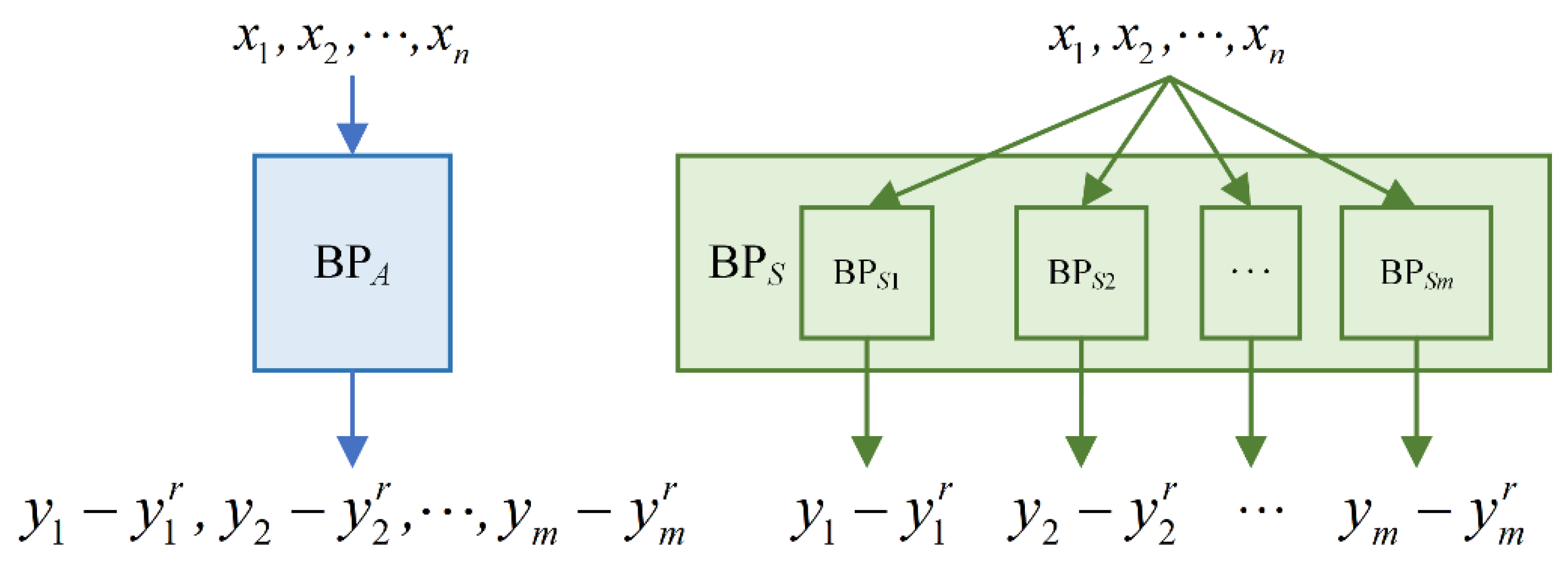
The effectiveness evaluation indicator system of remote sensing satellite cluster includes many indicators. If we only choose one BP neural network to train (BP_A architecture), the evaluation effect of the model is probably not good. Hence, a new architecture of BP neural network needs to be designed. It should be noted that the architecture design mentioned above refers to not changing the algorithm logic of the BP neural network, but only changing the output and number of the BP neural networks. The only difference between the BP_A architecture and the BP_S architectures is the number of BP neural networks used.

In this section, a new architecture of the BP neural network named BP_S architecture is designed, which can be seen in Figure 4. In BP_S architecture, the number of BP neural networks is the same as the number of indicators, which means that each indicator corresponds to a BP neural network model. In BP_S architecture, the input of each BP neural network model is related to the influencing factors of all indicators, and the output of each BP neural network model is related to the corresponding indicator. Compared with BP_S, there is only one BP neural network in BP_A architecture, which can be seen in Figure 4. In BP_A, the input of the BP neural network model is related to the influencing factors of all indicators, and the output of BP neural network model is a set of all indicators. It should be noted that BP_A architecture is introduced for comparison with BP_S architecture in this paper. Our goal is to highlight the advantages of BP_S architecture through comparison.

In BP_S architecture, the input of each BP neural network model is the influencing factors set of all indicators involved in the effectiveness evaluation indicator system of remote sensing satellite cluster, and the output of each BP neural network model is the residual value between the corresponding indicator value and the value predicted through multiple linear regression analysis of the corresponding indicator.

The multiple linear regression analysis model can be expressed by the following formula. The specific process of multiple linear regression analysis is as follows. Firstly, one multiple linear regression model is established for each indicator; then, it should be trained. Finally, the trained multiple linear regression model is used to predict the corresponding indicator value. It should be noted that the predicted indicator value is used to calculate the residual value mentioned in the previous paragraph.

$$y_i^r={\beta }_{i0}+{\beta }_{i1}{x}_1+\cdots +{\beta }_{in}{x}_n$$

(8)

3.2.2. Determination of Value Ranges of Hyperparameters

It is well known that the training effect of the BP neural network in BP_S architecture is affected directly by the selection of hyperparameters values. The hyperparameters mentioned in this paper include the type of activation function, the number of hidden layers, and the number of neurons in each hidden layer. The above three types of hyperparameters will produce too many different hyperparameters combinations. If the direct traversal method is used to find the optimal hyperparameter combination, the workload will be too heavy.

In this paper, the activation functions considered include softmax, poslin, satlin, logsig, tansig, satlins, radbas, elliotsig, and tribas. Considering the limitations of the complex effectiveness evaluation system for the remote sensing satellite cluster on the scale of the neural network, the value range of the number of hidden layers is [1, 3], and the value range of the number of neurons in each hidden layer is [0, 100].

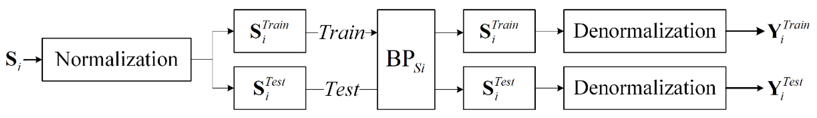
3.2.3. Model Training of BP Neural Network

The training process of BP neural network can be seen in Figure 5. The influencing factors of all indicators can be described as $X={\left[x_1,x_2,\cdots ,x_n\right]}^T$. BP_Si is the BP neural network in BP_S architecture established for the i-th indicator. The output of BP_Si can be described as $y_i-y_i^r$, where $y_i$ is the i-th indicator value and the $y_i^r$ is the value calculated through multiple linear regression analysis of the i-th indicator, which can be seen in Figure 4. $S_i$ is the sample space composed of $n_{Sample}$ samples. $S_i$ is a matrix of $n_{Sample}$ rows and $n+1$ columns, corresponding to $n$ inputs and 1 output of BP_Si.

The input and outputs of the sample space $S_i$ are normalized, and then $S_i$ is divided into training set $S_i^{Train}$ and test set $S_i^{Test}$ according to the ratio of $\sigma :1-\sigma$, where the number of rows of $S_i^{Train}$ and $S_i^{Test}$ are $\sigma \cdot n_{Sample}$ and $(1-\sigma )\cdot n_{Sample}$, respectively.

BP_Si is applied for sample input of training set $S_i^{Train}$ and test set $S_i^{Test}$, respectively. After that, the corresponding $y_i^r$ is added to the result predicted by BP_Si to obtain the indicator prediction results of the training set and the test set named ${\widehat{Y}}_i^{Train}$ and ${\widehat{Y}}_i^{Test}$, which is used to test the training and generalization performance of BP_Si.

The training performance of BP_Si is evaluated by calculating the mean square error (MSE) for the training set, which can be described as follows.

$$MSE={\displaystyle \sum _{i=1}^{n_{Index}}\left(\frac{w_i}{\sigma \cdot n_{Sample}}\times {\displaystyle \sum _{j=1}^{\sigma \cdot n_{Sample}}{(Y_{i,j}^{Train}-{\widehat{Y}}_{i,j}^{Train})}^2}\right)}$$

(9)

$$w_i={\left(\frac{1}{\max (Y_i^{Train})-\min (Y_i^{Train})}\right)}^2$$

(10)

The generalization performance of BP_Si is evaluated by calculating the mean absolute percentage error (MAPE). The MAPE of the test set of the i-th indicator is calculated as follows.

$$MAP{E}_i=\frac{1}{(1-\sigma )\cdot n_{Sample}}\times {\displaystyle \sum _{j=1}^{(1-\sigma )n_{Sample}}\left|\frac{Y_{i,j}^{Test}-{\widehat{Y}}_{i,j}^{Test}}{Y_{i,j}^{Test}}\right|}$$

(11)

3.3. The Multi-Round Traversal Method Based on the Three-Way Decision Theory for the Hyperparameter Combinations of the BP_S Neural Network

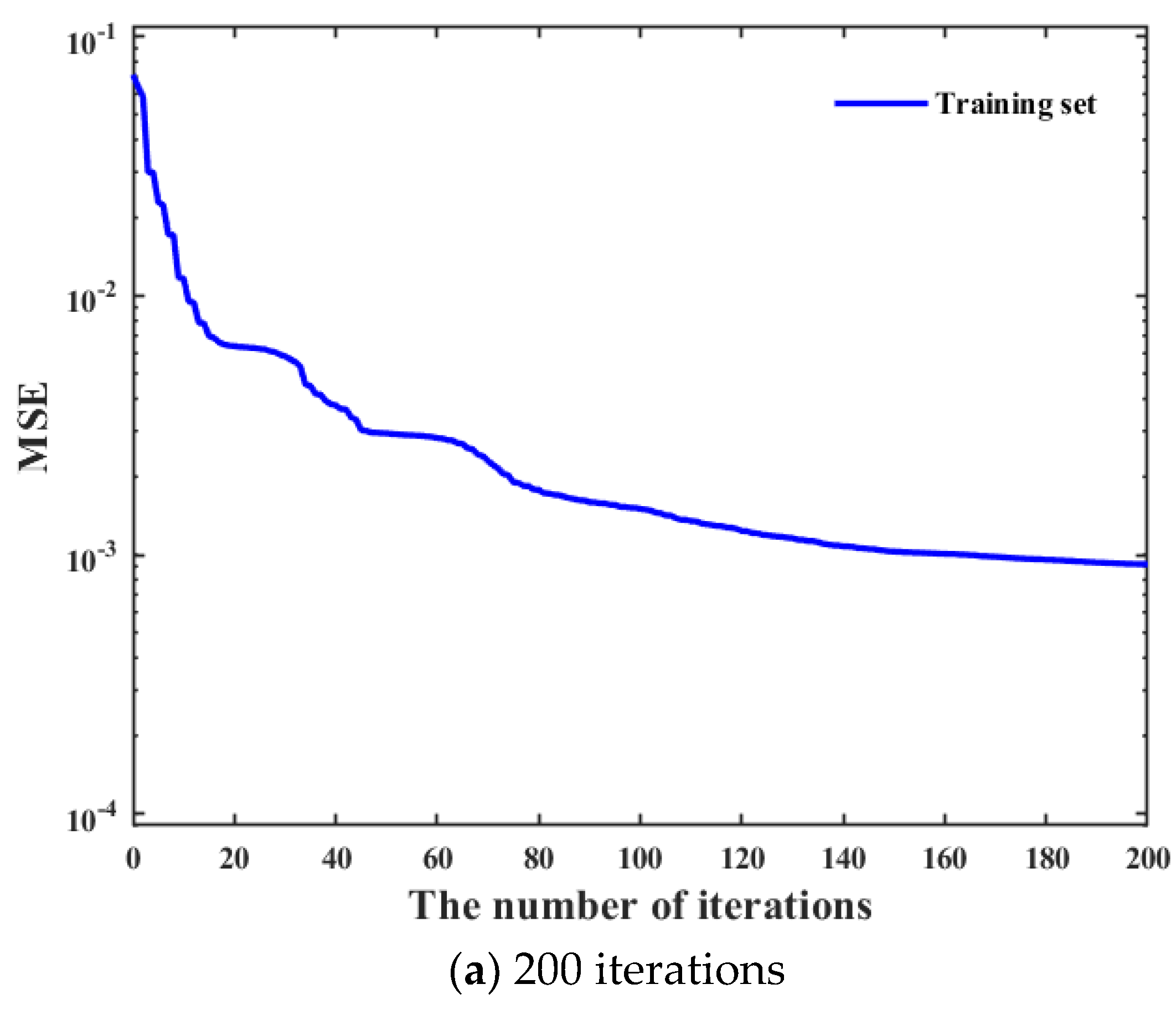
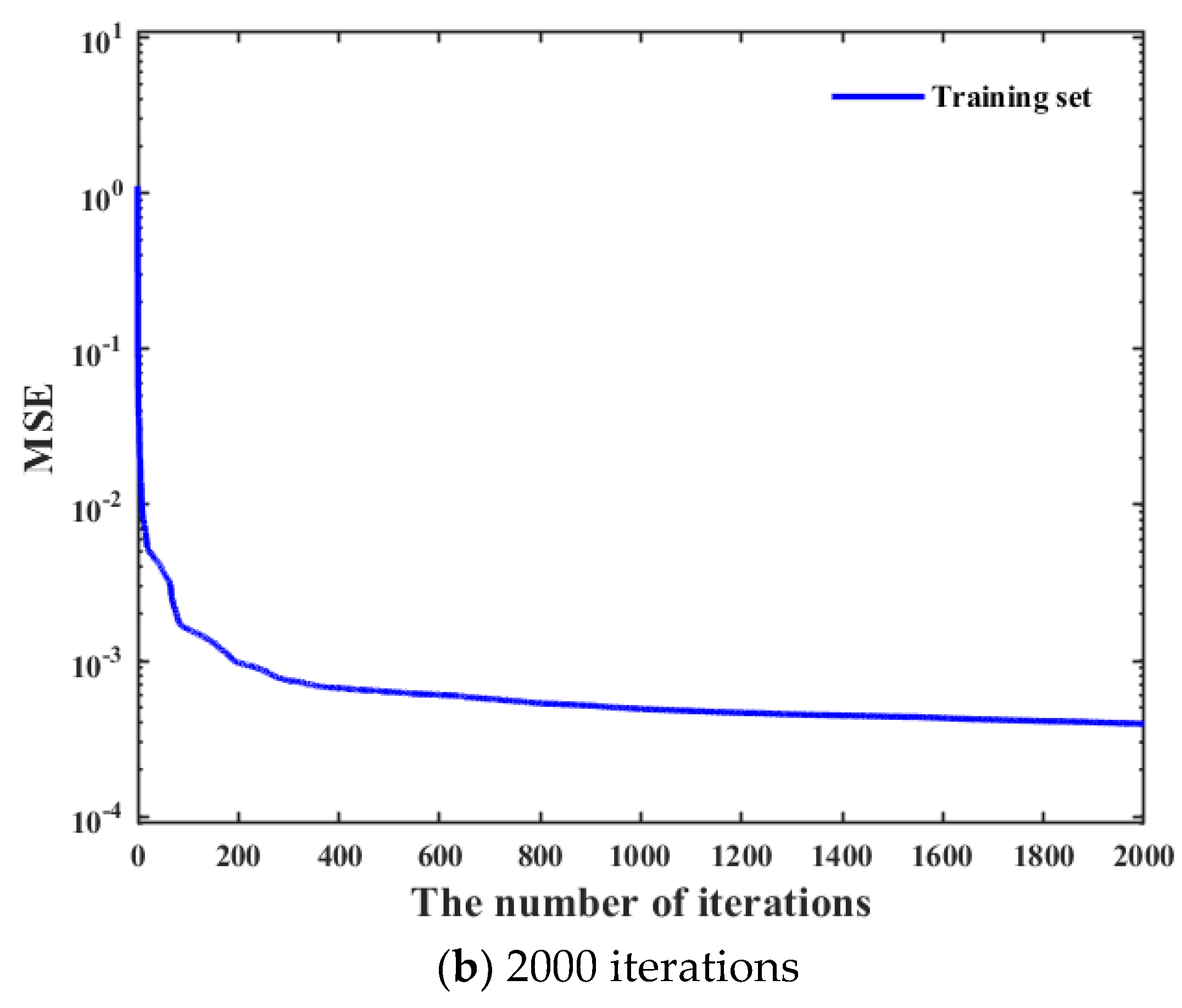
In order to improve the accuracy of the evaluation results predicted by BP_s architecture as much as possible, it is necessary to traverse all possible combinations of different types of activation functions, different numbers of hidden layers, and nodes in each hidden layer to obtain the optimal hyperparameters combination. Moreover, the training performance of the neural network often improves with the increase of the number of iterations. It can be seen in Figure 6 that the training performance of tracking time percentage indicator is significantly different under different iterations. Compared with 200 iterations, the training performance of tracking time percentage indicator under 2000 iterations is improved by about 50%, but the resource consumption of that is also increased by more than 10 times. Hence, it can be clearly found that the time cost is very high if all possible network design parameters combinations are directly traverse under high iterations. Hence, we hope to screen out some hyperparameter combinations with poor training effect as much as possible under low iterations, which can greatly shorten the overall model training time.

Three-way decision theory is a decision-making method based on human cognition. In the actual decision-making process, people can quickly make judgments about events that they have sufficient confidence in accepting or rejecting. For those events that cannot be decided immediately, people often delay their judgment, which is called delayed decisions [43].

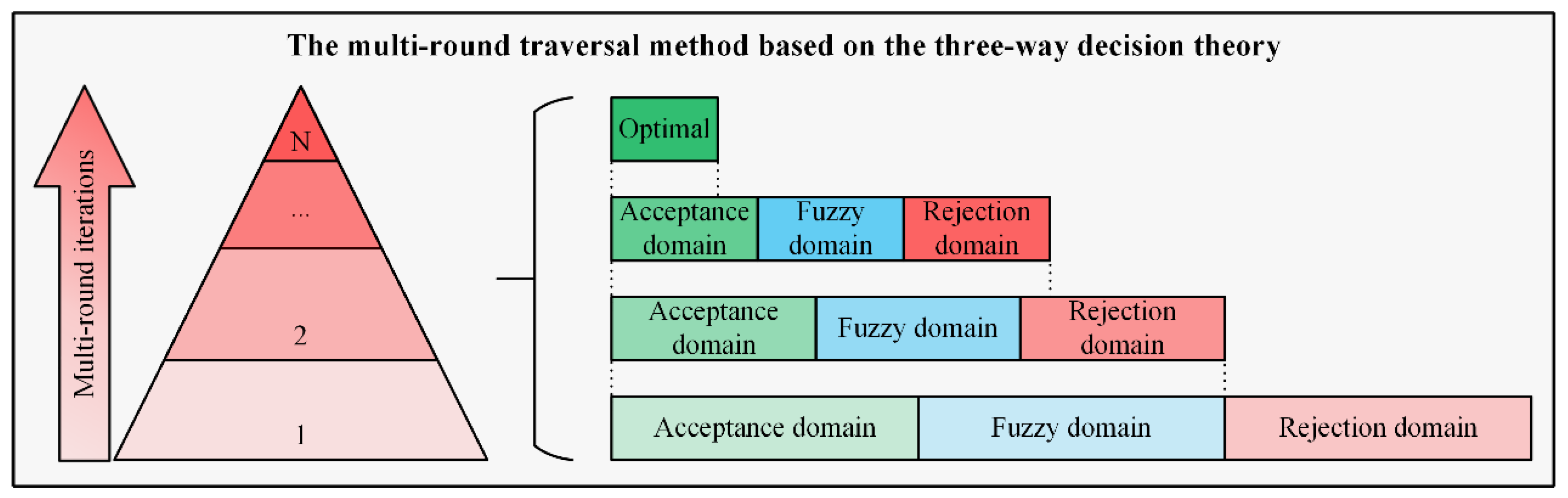
In this paper, the three-way decision theory is introduced into hyperparameter traversal combinations to find the optimal hyperparameter combination, which can be seen in Figure 7. It is quite time-consuming to directly traverse all hyperparameter combinations under high iterations. Hence, a multi-round traversal method is adopted. The multi-round traversal process is divided into multiple rounds based on the number of iterations. A portion of hyperparameter combinations with poor training performance is removed at each round of the multi-round traversal process, and the optimal hyperparameter combination can be obtained through multiple screening.

The specific screening process of the multi-round traversal method based on the three-way decision theory is shown in Figure 7. At each round of the multi-round traversal process, the training performance of the neural network with all different hyperparameter combinations is divided into three domains, which are defined as acceptance domain, fuzzy domain, and rejection domain according to the training performance from good to bad. Then, the hyperparameter combinations that belong to the rejection domain are removed, and the hyperparameter combinations that belong to the acceptance domain and the fuzzy domain are retained and continue to be screened at the next round of the multi-round traversal process. Most of the hyperparameter combinations with poor training performance are removed through the multi-round screening process, and then the rest of the hyperparameter combinations are traversed to find the optimal hyperparameter combinations set under high iterations. It should be noted that the top five hyperparameter combinations with the best training performance are combined to the optimal hyperparameter combinations set in this paper.

It should be noted that the prerequisite for applying three-way decision theory to neural network training is that the optimal hyperparameter combinations maintain certain consistency under different iterations. For example, if the training performance of the network with hyperparameter combination A is better than B under low iterations, then it will be also better under high iterations. Hence, the phenomenon that the optimal hyperparameter combination is incorrectly removed under low iterations can be effectively avoided, and the phenomenon that a large number of hyperparameter combinations with poor training performance are retained under low iterations can also be effectively avoided. Based on the BP_S architecture, seven BP_S neural networks are established for seven indicators. These seven BP_S neural networks are trained for 200, 400, 600, 800, 1000, 2000, and 3000 iterations, respectively. Different hyperparameter combinations are traversed for each BP_S neural network, which are described as follows. The activation functions include softmax, logsig, tansig, and radbas. The value range of the number of hidden layers is [1, 2]. The value range of the number of neurons in each hidden layer is [10, 20, 30, 40, 50]. Hence, there are a total of 40 different hyperparameter combinations. The training performance can be seen in Figure 8. It can be seen in Figure 8 that the ordinate displays the numbers of 40 hyperparameter combinations. Acceptance domains are marked with green; fuzzy domains are marked with blue, and rejection domains are marked with red.

It can be seen in Figure 8 that in most cases, the training performance of different hyperparameter combinations under different iterations maintains a high degree of consistency, which basically meets the prerequisites for using the three-way decision theory. However, there are two aspects worth noting. On the one hand, there are also a few special cases where the training performance of the hyperparameter combination with excellent training performance under low iterations becomes bad under high iterations. The above situation has no impact on the screening of the optimal hyperparameter combination, which can be ignored. On the other hand, there are also a few special cases where the training performance of the hyperparameter combination with bad training performance under low iterations becomes excellent under high iterations. The above situation may have a certain impact on the screening of the optimal hyperparameter combination. Hence, in order to prevent the occurrence of the above situation, we need to further research the number of rounds and the number of iterations per round for the multi-round iterative optimization process.

The training score for the j-th hyperparameter combination of the i-th indicator can be defined as follows.

$$t{s}_{i,j}^k=\left\{\begin{array}{ll}0\hfill & j\in \mathrm{Rejection}\mathrm{domain}\hfill \\ 1\hfill & j\in \mathrm{Fuzzy}\mathrm{domain}\hfill \\ 2\hfill & j\in \mathrm{Acceptance}\mathrm{domain}\hfill \end{array}\right.$$

(12)

where $1\le i\le n_{Index}$,$1\le j\le n_{Net}$.

The cumulative variation coefficient of the training performance between adjacent iterations k and k + 1 can be calculated as follows, which is abbreviated as the adjacent cumulative variation coefficient.

$$v{a}_j^{k,k+1}=\frac{1}{n_{Index}}{\displaystyle \sum _{i=1}^{n_{Index}}\frac{1}{n_{Net}}{\displaystyle \sum _{j=1}^{n_{Net}}(t{s}_{i,j}^k-}}t{s}_{i,j}^{k+1}{)}^2$$

(13)

where k is the number of iterations, $k=100,200,\cdots ,n_{Epoch}$.

The cumulative variation coefficient of the training performance between current iteration k and the max iteration $n_{Epoch}$ can be calculated as follows, which is abbreviated as the optimal cumulative variation coefficient.

$$v{a}_j^{k,n_{Epoch}}=\frac{1}{n_{Index}}{\displaystyle \sum _{i=1}^{n_{Index}}\frac{1}{n_{Net}}{\displaystyle \sum _{j=1}^{n_{Net}}(t{s}_{i,j}^k-}}t{s}_{i,j}^{Epoch}{)}^2$$

(14)

The number of rounds and the number of iterations per round for the multi-round iterative optimization process are determined by comparing the cumulative variation coefficient of the training performance between different iterations.

4. Results and Discussion

4.1. Experimental Parameter Configuration

The observation scene of remote sensing satellite cluster on moving targets is established based on the related reference [8]. The orbital parameters of the remote sensing satellite cluster are set according to the configuration of Walker constellation, which can be seen in Table 1.

The inputs and their value ranges for neural network training are defined as follows, which can be seen in

Table 2. The inputs and their value ranges for neural network training.

Inputs	Value Range
Simulation start time $t_{Start}$	From 0:00 on 1 January 2020 to 0:00 on 1 January 2023
Discovery mission coefficient $k_{Discovery}$	0~1
Identification mission coefficient $k_{Identification}$	0~1
Confirmation mission coefficient $k_{Confirmation}$	0~1
Target loss determination time $T_{Lost}$	5000~10,000
Tracking mission time coefficient	0~1

. The core influencing factors involved in satellite cluster mission scheduling are chosen to be the inputs of the neural network.

The entire sample set is divided into training sets and testing sets in a 1:4 ratio, which means that $\sigma =0.8$. The maximum number of iterations is 10,000. The activation functions of the hidden layer include softmax, poslin, satlin, logsig, tansig, satlins, radbas, elliotsig, and tribus. Purelin is chosen to be the activation function of the output layer. Considering the limitations of network size, the value range of the number of hidden layers is [1–3], and the value range of the number of neurons in each hidden layer is [10, 20, 30, 40, 50, 60, 70, 80, 90, 100].

A total of 6600 samples were collected by using 40 8-core i7 9700 k CPU computers. Each sample needs to be simulated 50 times to calculate the average of all indicators. Hence, 330,000 simulations take about 3 months in total.

4.2. Verification of the Effectiveness of the Multi-Round Traversal Method Based on the Three-Way Decision Theory

In this section, the effectiveness of applying the three-way decision theory to the iterative optimization method for hyperparameters of BP_S neural network is verified. The number of samples is 6000. The number of hidden layers is 1. The value range of the number of neurons in the hidden layer is [20, 40, 60, 80, 100]. The activation functions of the hidden layer include softmax, poslin, satlin, logsig, tansig, satlins, radbas, elliotsig, and tribas. Purelin is chosen to be the activation function of the output layer.

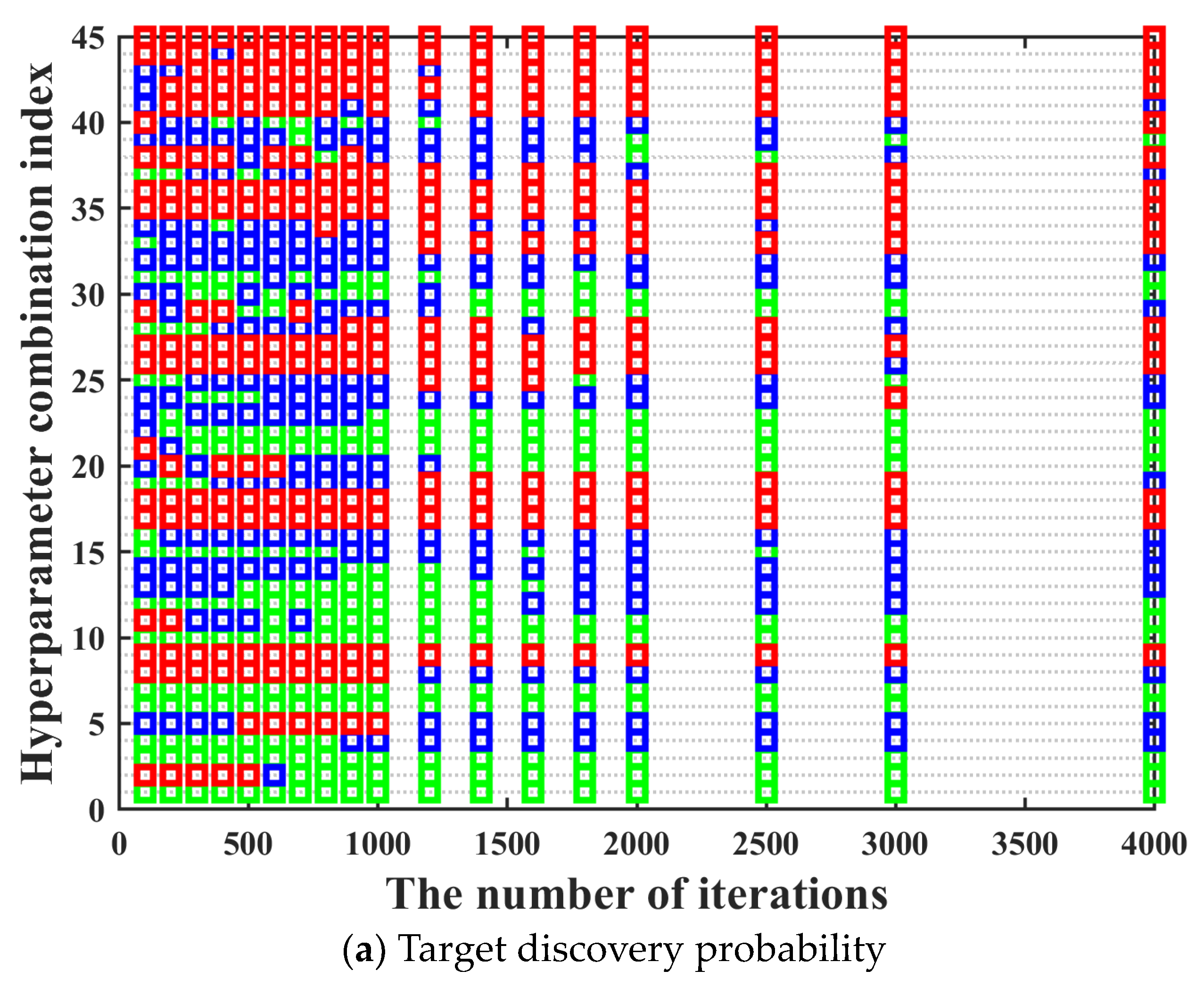
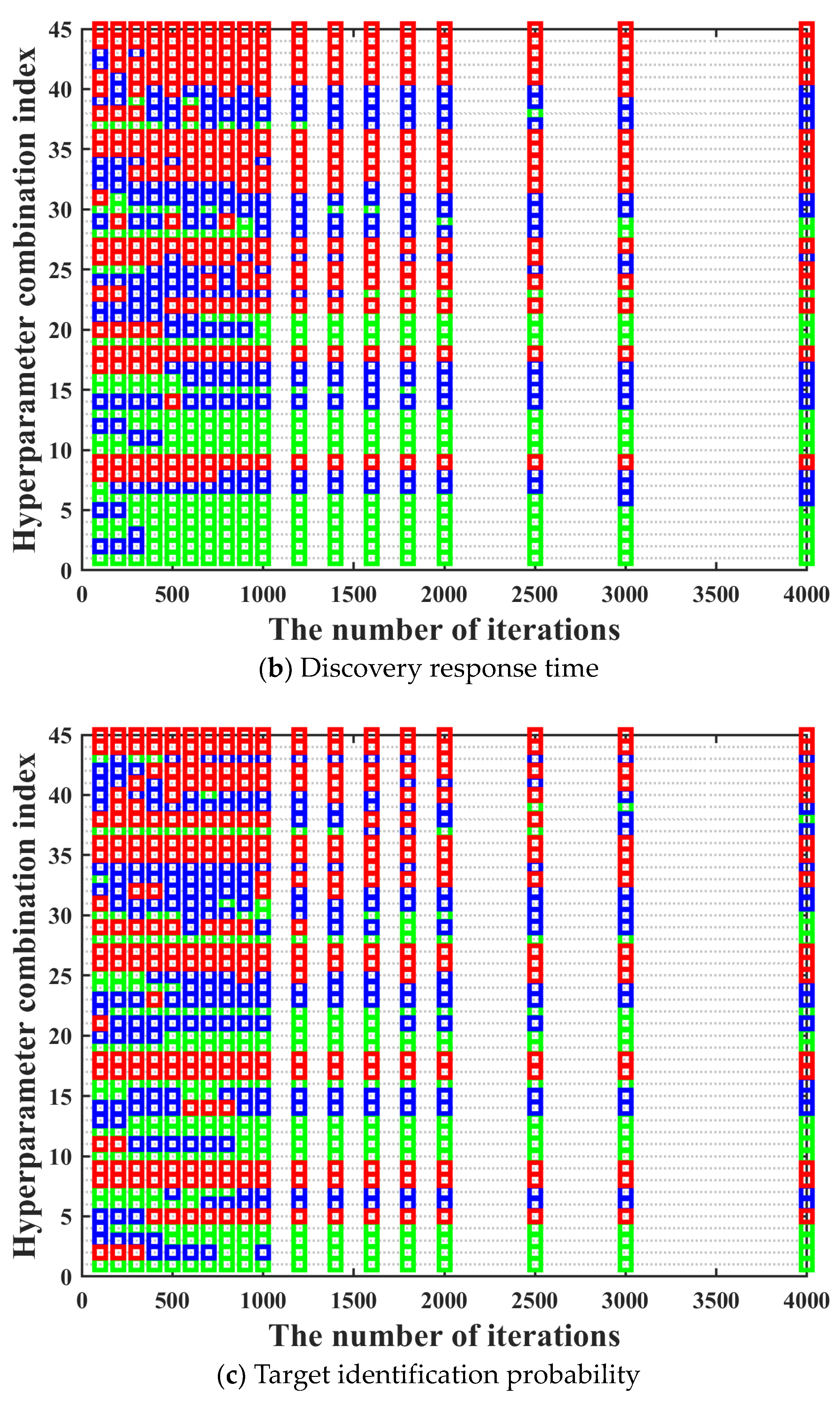
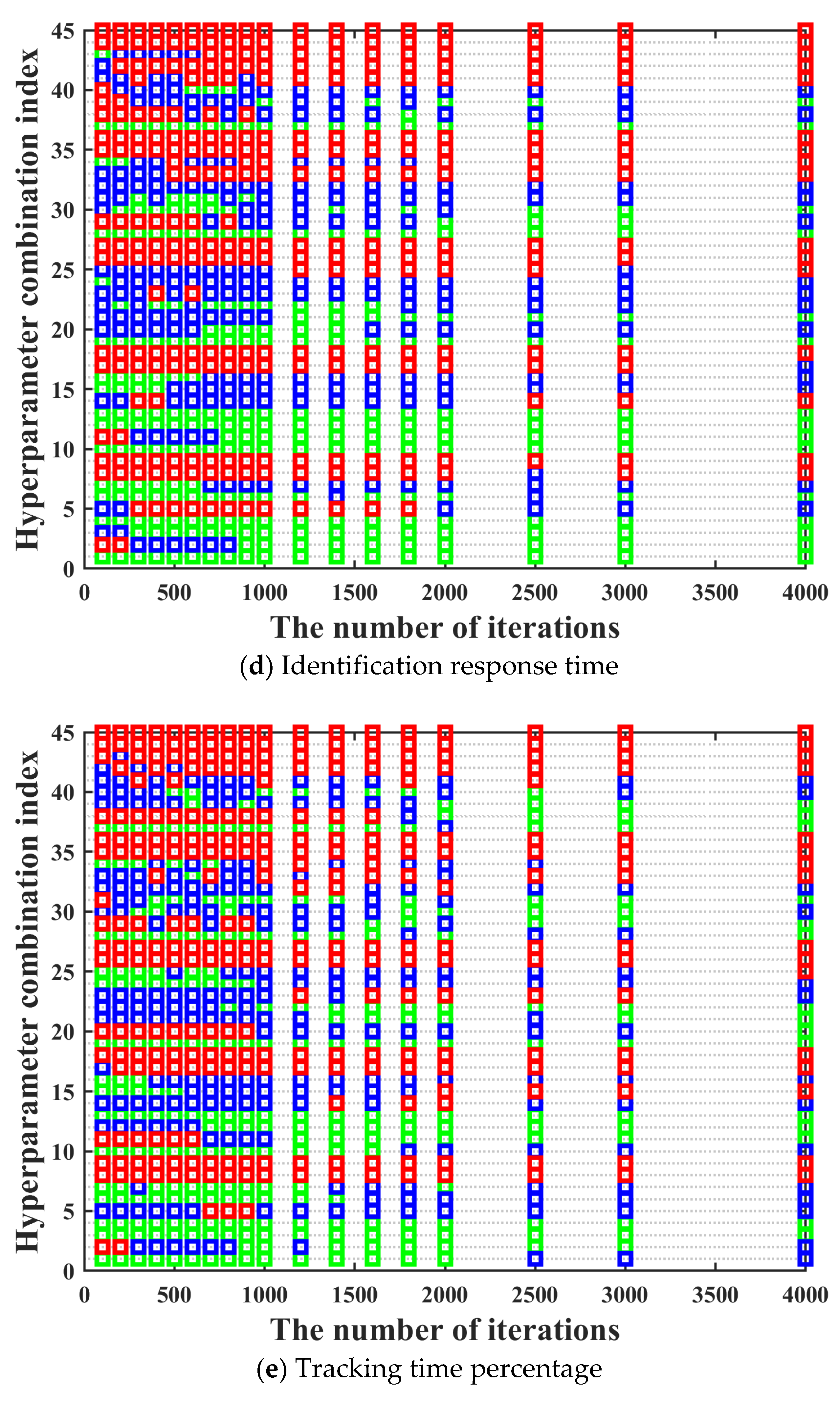
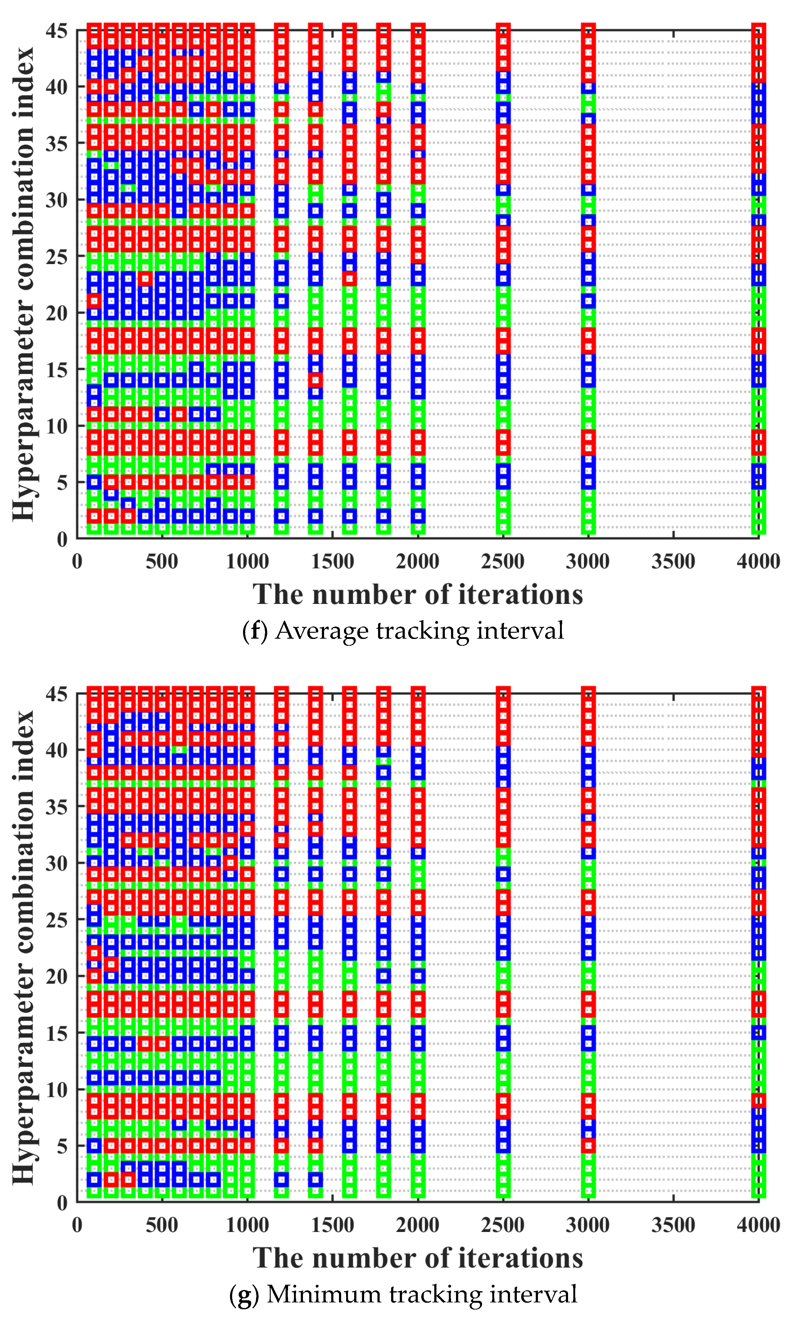
Moreover, in order to make the training performance of hyperparameter combinations under different iterations to maintain a high degree of consistency as much as possible, the number of rounds and the number of iterations per round for the multi-round iterative optimization process are determined by comparing the cumulative variation coefficient of the training performance between different iterations in this section. The value range of iteration number is [100, 200, 300, 400, 500, 600, 700, 800, 900, 1000, 1200, 1400, 1600, 1800, 2000, 2500, 3000, 4000]. The training performance of all hyperparameter combinations under different iterations is shown in Figure 9.

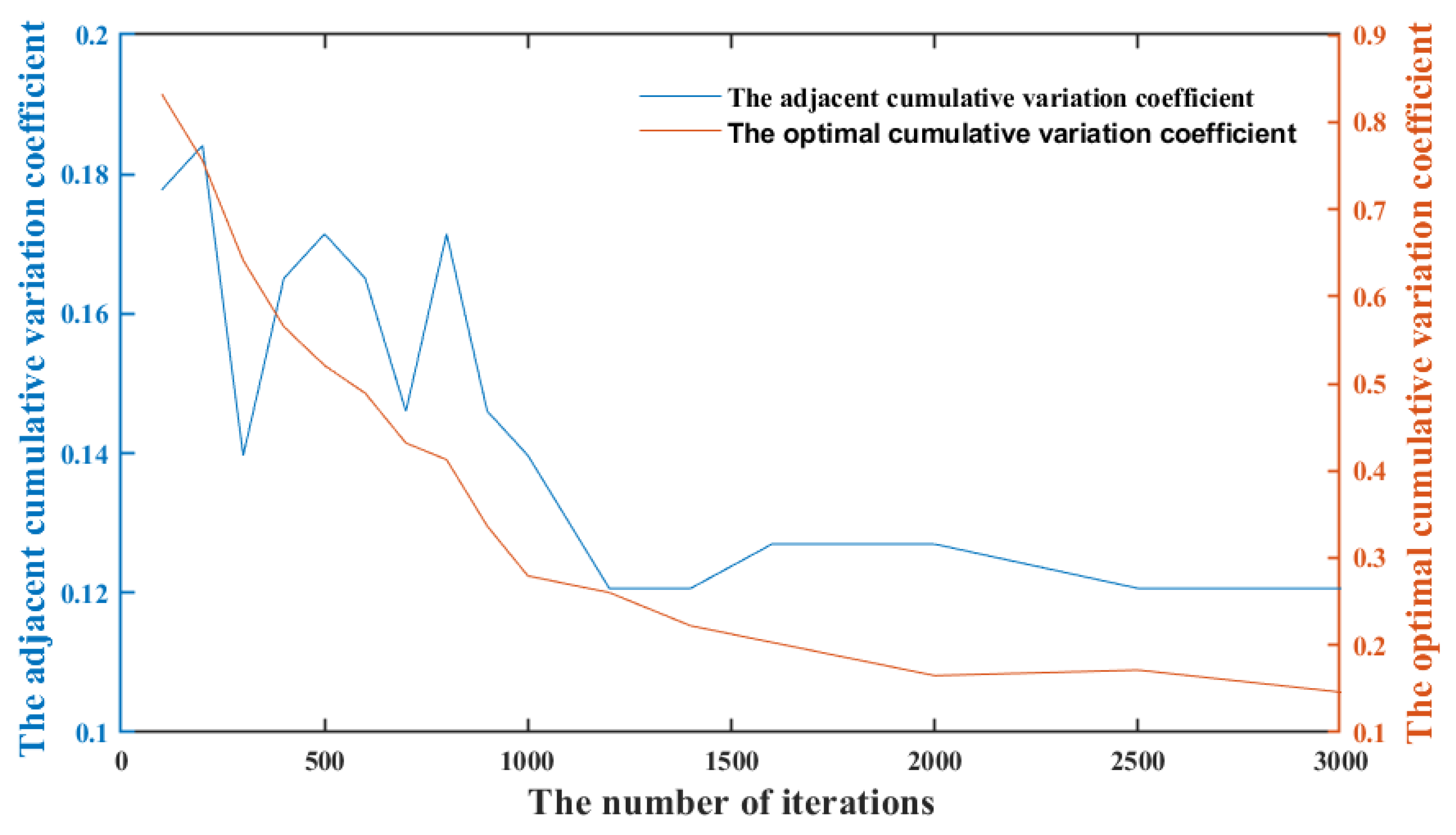
It can be seen in Figure 9 that after the hyperparameter combination is determined, its training performance maintains good consistency under different iterations. The only situation we need to pay attention to is that there are also a few special cases where the training performance of the hyperparameter combination with bad training performance under low iterations becomes excellent under high iterations. In order to prevent the occurrence of the above situation, we need to further determine the most suitable number of rounds and the number of iterations per round for the multi-round iterative optimization process by comparing the adjacent and optimal cumulative variation coefficient calculated under different iterations. The adjacent cumulative variation coefficient $v{a}_j^{k,k+1}$ and optimal cumulative variation coefficient $v{a}_j^{k,n_{Epoch}}$ are calculated, which can be seen in Figure 10.

It should be noted that we want to find the optimal hyperparameter combinations set through the three-way decision theory in this paper, not only one optimal hyperparameter combination. It can be known from Figure 9 that there may be situations where the training performance of rather a small number of hyperparameter combinations cannot maintain good consistency under different iterations. Hence, it is the most suitable for the actual situation to screen a part of the optimal hyperparameter combinations set through the three-branch decision theory as the relatively optimal combinations. Moreover, it can be known from

Table 3. The optimal hyperparameter combinations set of seven BP_A neural networks.

Neural Network Name	Number	MSE	The Number of Hidden Layers	The Number of Neurons in Each Hidden Layer	The Activation Function of the Hidden Layer
BPA	1	0.002063	2	30	tansig
	2	0.002210	2	40	radbas
	3	0.002288	1	30	radbas
	4	0.002371	2	20	tansig
	5	0.002382	2	30	radbas

that the difference in training performance between hyperparameter combinations in the optimal hyperparameter combinations set is not significant, which can be ignored.

It can be seen in Figure 10 that as the number of iterations increases, both the cumulative variation coefficient of the training performance $v{a}_j^{k,k+1}$ and $v{a}_j^{k,n_{Epoch}}$ show a downward trend. Compared with the cumulative variation coefficient of the training performance $v{a}_j^{k,n_{Epoch}}$, the cumulative variation coefficient of the training performance $v{a}_j^{k,k+1}$ first fluctuates and decreases, then steadily decreases, and finally approaches zero. The cumulative variation coefficient of the training performance between adjacent iterations $v{a}_j^{k,k+1}$ fluctuates significantly when the number of iterations is less than 900, and it tends to decline steadily when the number of iterations exceeds 900, which means that the error in dividing the rejection domain and the acceptance domain almost disappears. When the number of iterations exceeds 1500, both the cumulative variation coefficients of the training performance $v{a}_j^{k,k+1}$ and $v{a}_j^{k,n_{Epoch}}$ still decrease steadily, but the rate of decrease slows down significantly, which means that the optimal hyperparameter combinations set is only adjusted in adjacent domains. When the number of iterations exceeds around 2500, both the cumulative variation coefficients of the training performance $v{a}_j^{k,k+1}$ and $v{a}_j^{k,n_{Epoch}}$ remain basically unchanged, which means that the optimal hyperparameter combinations set tends to stabilize.

According to the above analysis, the number of rounds is determined as 4. The number of iterations for the first round is 900, and the first two-thirds of the hyperparameter combinations which belong to the acceptance domain and fuzzy domain are selected for the next round. The number of iterations for the second round is 1500, and the first two-thirds of the hyperparameter combinations which belong to the acceptance domain and fuzzy domain are selected for the next round. The number of iterations for the third round is 2500, and the first one-third of the hyperparameter combinations which belong to the acceptance domain are selected for the final round. The number of iterations for the final round is 4000, and a part of hyperparameter combinations is selected as the optimal hyperparameter combinations set.

The time consumption of the direct traversal method and the multi-round traversal method based on the three-way decision theory is calculated and compared. On the premise that both methods achieve the same training effect, the time consumption of the direct traversal method and the three-way decision theory step-by-step traversal method is 14.85 h and 4.28 h, respectively. Compared with the direct traversal method, the time consumption of the multi-round traversal method based on the three-way decision theory is decreased by more than 70%. This is due to the fact that all hyperparameter combinations need to be trained for 4000 iterations in the direct traversal method. Compared with the direct traversal method, only a few of hyperparameter combinations need to be trained for 4000 iterations, and the rest of the hyperparameter combinations are screened out before 4000 iterations in the multi-round traversal method based on the three-way decision theory. Hence, the total training time can be greatly shortened.

4.3. The Training Accuracy and Generalization Ability of the BP_S Trained by the Multi-Round Traversal Method Based on the Three-Way Decision Theory

In Section 4.2, the effectiveness of the multi-round traversal method based on the three-way decision theory is verified. Hence in this section, the optimal hyperparameter combinations set can be obtained by using multi-round traversal method based on the three-way decision theory. The value range of the number of hidden layers is [1–3], and the value range of the number of neurons in each hidden layer is [10, 20, 30, 40, 50, 60, 70, 80, 90, 100]. The activation functions of the hidden layer include softmax, poslin, satlin, logsig, tansig, satlins, radbas, elliotsig, and tribas. Purelin is chosen to be the activation function of the output layer. Hence, there are 270 different hyperparameter combinations.

One BP neural network is established for seven indicators involved in Section 2, which is named BP_A. In BP_A architecture, the optimal hyperparameter combinations set of each BP neural network can be obtained after training each BP neural network, which can be seen in Table 3. For the BP neural network in BP_A architecture, the top five hyperparameter combinations with the best training performance are combined to the optimal hyperparameter combinations set. It can be seen in Table 3 that the MSEs of these top five hyperparameter combinations with the best training performance are not significantly different in BP_A architecture.

In BP_S architecture, seven BP neural networks are established for seven indicators involved in Section 2, which are named BP_S1, BP_S2, BP_S3, BP_S4, BP_S5, BP_S6, and BP_S7, respectively. The optimal hyperparameter combinations set of each BP neural network can be obtained after training each BP neural network, which can be seen in

Table 4. The optimal hyperparameter combinations set of seven BP_S neural networks.

Neural Network Name	Number	MSE	The Number of Hidden Layers	The Number of Neurons in Each Hidden Layer	The Activation Function of the Hidden Layer
BPS1	1	0.002435	2	10	tansig
	2	0.002943	2	20	logsig
	3	0.003504	1	30	poslin
	4	0.003555	2	30	tansig
	5	0.003563	1	20	radbas
BPS2	1	0.002882	1	20	tansig
	2	0.002983	2	10	satlin
	3	0.003100	3	10	softmax
	4	0.003106	1	10	logsig
	5	0.003165	2	10	tansig
BPS3	1	0.001493	2	50	softmax
	2	0.001500	2	20	softmax
	3	0.001526	2	20	tansig
	4	0.001533	2	30	softmax
	5	0.001557	2	10	logsig
BPS4	1	0.001190	2	20	softmax
	2	0.001192	1	50	softmax
	3	0.001208	1	30	softmax
	4	0.001212	2	50	softmax
	5	0.001222	1	20	softmax
BPS5	1	0.000178	2	10	logsig
	2	0.000190	2	30	tansig
	3	0.000197	1	40	radbas
	4	0.000198	1	30	softmax
	5	0.000210	1	50	softmax
BPS6	1	0.000731	2	20	tansig
	2	0.000809	1	40	radbas
	3	0.000844	1	20	tansig
	4	0.000869	1	50	radbas
	5	0.000899	2	20	radbas
BPS7	1	0.001568	2	30	softmax
	2	0.001570	1	20	softmax
	3	0.001585	1	50	softmax
	4	0.001592	2	20	logsig
	5	0.001598	2	10	radbas

. For each BP neural network in BP_S architecture, the top five hyperparameter combinations with the best training performance are combined to the optimal hyperparameter combinations set. It can be seen in Table 4 that the MSEs of these top five hyperparameter combinations with the best training performance are not significantly different in BP_S architecture.

The generalization abilities of the BP_S neural network and the BP_A neural network with the optimal hyperparameter combination are compared, which can be seen in

Table 5. The generalization abilities of BP_S neural network and the BP_A neural network with the optimal hyperparameter combination. (Some values are set in bold to highlight the advantages of BP_S over BP_A).

Number	Indicator	MAPE
		BPA	BPS
1	Target discovery probability	0.0563	0.0504
2	Discovery response time	0.1149	0.1205
3	Target identification probability	0.0600	0.0597
4	Identification response time	0.0506	0.0508
5	Tracking time percentage	0.0794	0.0642
6	Average tracking interval	0.0389	0.0383
7	Minimum tracking interval	0.0939	0.0958

.

It can be seen in Table 5 that compared with the BP neural networks in BP_S architecture corresponding to the target discovery probability indicator and the tracking time percentage indicator, the MAPEs of the BP neural network in BP_A architecture corresponding to the target discovery probability indicator and the tracking time percentage indicator are significantly worse. Moreover, the MAPEs of the BP neural networks in BP_S architecture corresponding to the rest five indicators are basically the same as that of the BP neural networks in BP_A architecture corresponding to the rest five indicators. Based on a comprehensive analysis of the MAPEs of the BP_S architecture and BP_A architecture corresponding to seven indicators, BP_S architecture is better than BP_A architecture. It is due to the fact that compared with the BP_A architecture, the BP_S architecture is more targeted. In BP_S architecture, one BP neural network is established for one indicator, which means that one BP neural network serves one indicator. However, in BP_A architecture, one BP neural network serves seven indicators, which means that the BP_A architecture is difficult to meet the high-precision requirements of all indicators. It is undoubtedly true that the model training time of the BP_A architecture is much shorter than that of the BP_S architecture. However, the precision of the BP_A architecture is much lower than that of the BP_S architecture. The main goal of this paper is to improve the prediction accuracy of the neural network model as much as possible. On this premise, we try to minimize the model training time as much as possible.

Hence, it can be concluded from the above analysis that the BP_S architecture is superior to the BP_A architecture from the perspective of the generalization ability comparison results of all indicators. The main reasons are as follows. On the one hand, the optimal weight parameters of each indicator are different. If the BP_A architecture is chosen, the number of neural network models will be only one. We cannot guarantee that the optimal weight parameters obtained through model training are optimal for each indicator. On the other hand, the optimal hyperparameter combination of each indicator is different. If the BP_A architecture is chosen, the optimal hyperparameter combinations set obtained through model training will not be optimal for each indicator. If the BP_S architecture is chosen, that is, the corresponding neural network model for each indicator is established and trained, respectively, the optimal weight parameters and the optimal hyperparameter combinations for each corresponding neural network model will be obtained through model training.

4.4. Comparison with Traditional Simulation Calculation Method

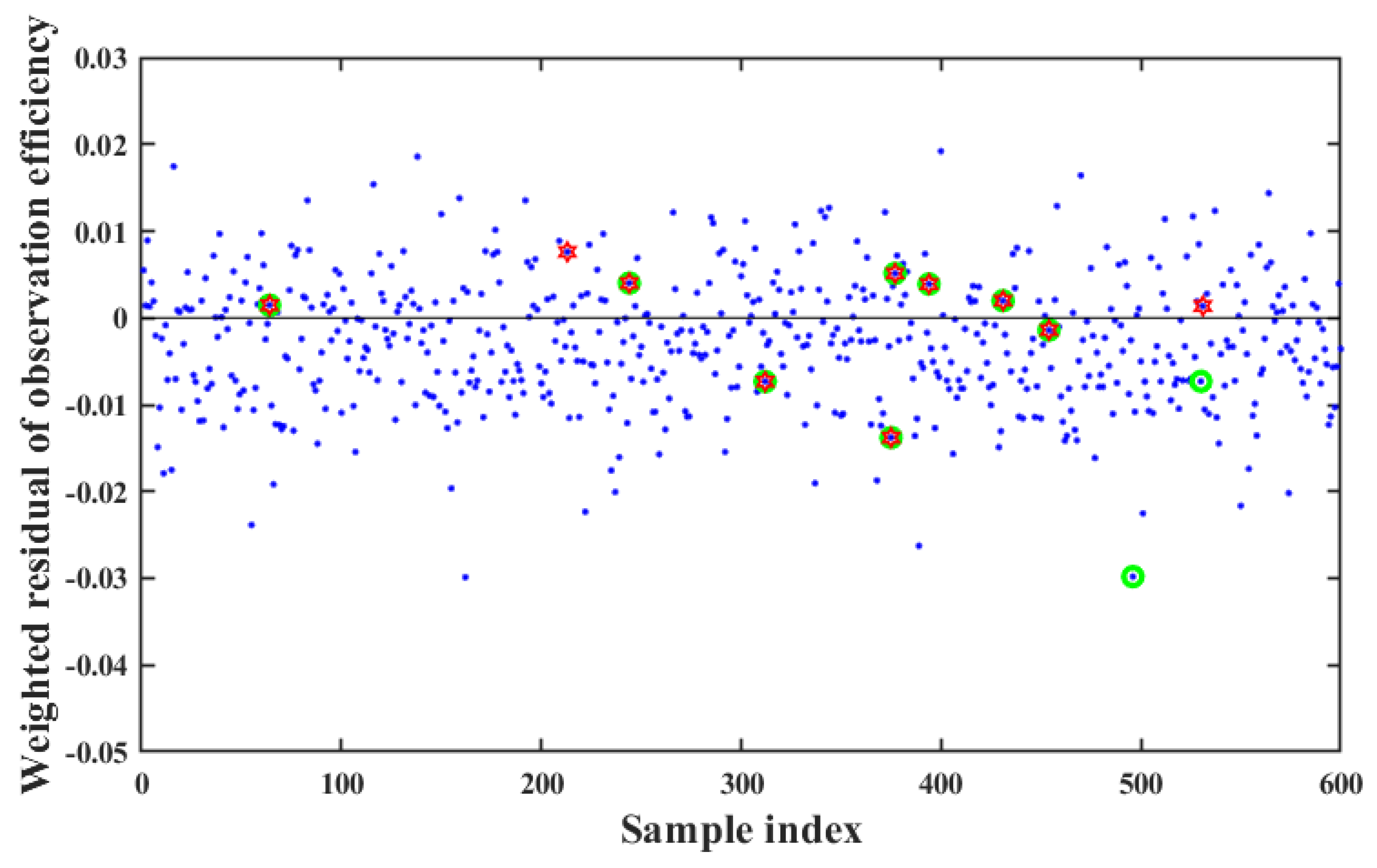
Some 600 samples are generated within the neighborhood range of training parameters randomly, and all indicator values calculated through the simulation model and the neural network model are weighted, summed, and then compared, respectively, which can be seen in Figure 11. It should be noted that the neural network model mentioned above refers to the model with BP_S architecture trained by using multi-round traversal method. The ordinate in Figure 11 is defined as the difference between the weighted summation values of indicators calculated by the neural network model and the simulation model. The optimal 10 samples obtained through neural network models and simulation models are labeled with two different colors, green and red, respectively. It can be seen from Figure 11 that the difference between the weighted summation values of indicators calculated by the neural network model and the simulation model is basically within 0.02, which means that the weighted summation values of indicators calculated by the neural network and simulation model are basically same. At the same time, 9 out of the 10 optimal samples obtained using the neural network model and the simulation model remained consistent, which indicates that the effectiveness of the effectiveness evaluation by using the neural network model. Moreover, the time consumption between the neural network model and the simulation model are compared, which can be seen in

Table 6. The time consumption comparison between the neural network model and the simulation model.

	Time Consumption/Days
Neural network model	10.45
Simulation model	0.00003

. The simulation model takes approximately 10.45 days to predict the effectiveness evaluation results, However, the effectiveness evaluation results can be predicted in real-time (0.00003 days) through the neural network model.

In summary, the effectiveness evaluation of a remote-sensing satellite cluster system through the neural network model cannot only obtain the same effectiveness evaluation results as the simulation model but also greatly improve the operational efficiency of the model. It has the ability to quickly and accurately evaluate.

5. Conclusions

The BP neural network is introduced into the effectiveness evaluation for remote sensing satellite cluster system in this paper. We have made two improvements to the BP neural network in this paper. One is that a new architecture for the BP neural network named BP_S is designed based on the effectiveness evaluation indicator system of remote sensing satellite cluster. In BP_S architecture, one BP neural network is established for each indicator involved in the effectiveness evaluation indicator system of the remote-sensing satellite cluster, respectively, which can effectively improve prediction accuracy. The results show that based on a comprehensive analysis of the generalization ability of the BP_S and BP_A neural networks corresponding to seven indicators, the BP_S we designed is better than traditional method BP_A, especially for the tracking time percentage indicator. Compared with the BP neural network in BP_S architecture corresponding to the tracking time percentage indicator, the MAPE of the BP neural network in BP_A architecture corresponding to the tracking time percentage indicator is significantly worse, which increase exceeds 20%. Moreover, the multi-round traversal method based on the three-way decision theory is designed in order to solve the problem of the low efficiency in model training. The results show that compared with the direct traversal method, the model training time of the multi-round traversal method based on the three-way decision theory is decreased by more than 70%. Finally, the neural network model method we designed is compared with the traditional simulation calculation method. The neural network model we designed can not only obtain the same effectiveness evaluation results as the simulation model but also greatly improve the operational efficiency of the model. It has the ability to quickly and accurately evaluate.

In the future, we will consider conducting correlation analysis on the input and output of the sample, investigating which input parameters have an impact on the output parameters, and eliminating irrelevant input parameters to further reduce the model training time.