Article

Early Detection of Wheat Yellow Rust Disease and Its Impact on Terminal Yield with Multi-Spectral UAV-Imagery

1
Taylor Geospatial Institute, St. Louis, MO 63108, USA
2
Department of Earth and Atmospheric Sciences, Saint Louis University, St. Louis, MO 63108, USA
3
Department of Aviation, University of Central Missouri, Warrensburg, MO 64093, USA
4
GDM Seeds, Chacabuco, Buenos Aires 6740, Argentina
*
Author to whom correspondence should be addressed.
Remote Sens. 2023, 15(13), 3301; https://doi.org/10.3390/rs15133301
Submission received: 18 May 2023 / Revised: 17 June 2023 / Accepted: 21 June 2023 / Published: 27 June 2023
(This article belongs to the Section Biogeosciences Remote Sensing)

Abstract

:
The food production system is vulnerable to diseases more than ever, and the threat is increasing in an era of climate change that creates more favorable conditions for emerging diseases. Fortunately, scientists and engineers are making great strides to introduce farming innovations to tackle the challenge. Unmanned aerial vehicle (UAV) remote sensing is among the innovations and thus is widely applied for crop health monitoring and phenotyping. This study demonstrated the versatility of aerial remote sensing in diagnosing yellow rust infection in spring wheats in a timely manner and determining an intervenable period to prevent yield loss. A small UAV equipped with an aerial multispectral sensor periodically flew over, and collected remotely sensed images of, an experimental field in Chacabuco (−34.64; −60.46), Argentina during the 2021 growing season. Post-collection images at the plot level were engaged in a thorough feature-engineering process by handcrafting disease-centric vegetation indices (VIs) from the spectral dimension, and grey-level co-occurrence matrix (GLCM) texture features from the spatial dimension. A machine learning pipeline entailing a support vector machine (SVM), random forest (RF), and multilayer perceptron (MLP) was constructed to identify locations of healthy, mild infection, and severe infection plots in the field. A custom 3-dimensional convolutional neural network (3D-CNN) relying on the feature learning mechanism was an alternative prediction method. The study found red-edge (690–740 nm) and near infrared (NIR) (740–1000 nm) as vital spectral bands for distinguishing healthy and severely infected wheats. The carotenoid reflectance index 2 (CRI2), soil-adjusted vegetation index 2 (SAVI2), and GLCM contrast texture at an optimal distance d = 5 and angular direction θ = 135° were the most correlated features. The 3D-CNN-based wheat disease monitoring performed at 60% detection accuracy as early as 40 days after sowing (DAS), when crops were tillering, increasing to 71% and 77% at the later booting and flowering stages (100–120 DAS), and reaching a peak accuracy of 79% for the spectral-spatio-temporal fused data model. The success of early disease diagnosis from low-cost multispectral UAVs not only shed new light on crop breeding and pathology but also aided crop growers by informing them of a prevention period that could potentially preserve 3–7% of the yield at the confidence level of 95%.

1. Introduction

Wheat (Triticum aestivum L.) is among the most widely grown crops but very vulnerable to various pests and diseases such as yellow rust, powdery mildew, aphids, etc., which devastate the harvesting yield and thus endanger the world’s future food security and sustainability needs [1]. Timely, effective, and precise disease monitoring for the crop is of paramount importance to properly intervene and prevent significant economic losses in farming practice. This prevention can be conventionally accomplished by chemical treatment, which is a calendar-based application of fungicides irrespective of disease development and risks. Such a control strategy, however, not only incurs a high cost (economically) but also increases the likelihood of groundwater contamination (environmentally) and chemical residues in agricultural products (socially) [2]. By a more sustainable crop management strategy, crop growers can simply avoid susceptible wheat varieties before planting, or by a decision-based practice, detecting and controlling diseases as early as standing crops being invaded, to halt the build-ups in the crop during the growing season.
The traditional approach to detecting the presence of abiotic stress in plants involves an invasive sampling followed by a lab-based verification, which is labor-intensive and highly subjective to sampling bias, and thus unsuitable for large-scale and temporal monitoring. On the contrary, with its user-defined spatial-spectral-temporal resolution, cost-friendliness and flexibility, unmanned aircraft vehicle (UAV) remote sensing, equipped with miniaturized and mobile sensors such as red-green-blue (RGB), multispectral, hyperspectral, thermal, radar, etc., is gathering ever-increasing interest in the search for sustainable disease control [3,4,5,6]. Complementing the advent of UAV hardware platforms, the revolution in location-aware science and artificial intelligence (GeoAI) has fundamentally changed the methods of data curation as well as the transformation of the data into actionable information to alert farmers to the danger of a site-specific disease invasion in a timely manner.
The focal investigation of this work was wheat yellow rust (Puccinia striiformis f. sp. tritici), which is one of the serious diseases occurring in most wheat crops in normal environmental and meteorological conditions of plant growth. The most visible symptom of the infection, making it easily diagnosed, is yellow-colored stripes on wheat leaves. The rust stripes are usually 2 or 3 mm wide, running parallel to the leaf veins [2]. This epidemic disease can significantly reduce the yield and quality, statistically by 10–30%, which amounts to a USD 5 billion loss worldwide each year [7,8]. In theory, infection by disease inevitably alters certain physical, physiological, and biochemical properties of plants, and as a result, the photosynthesis pattern would change accordingly and reflect the change in the radiant energy absorption and reflectance rate, which could be measured by remote sensors such as multispectral and hyperspectral imagers [1,9], spectrographs [2], spectroscopes [10], spectrometers [11,12], or spectrophotometers [13]. For example, yellow rust brings typical changes in wheat vigor, pigments, chlorophyll, and water stress. [14] found that chlorophyll content reduction could be observed in the visible (VIS) and red-edge spectral wavelengths (550 nm; 650–720 nm). Altered pigments of infected plants are likely to reshape the VIS and near-infrared (NIR) (680–800 nm) signals [14]. Most of the aforementioned studies monitored the yellow rust disease development on the leaf scale at the ground or near-surface level. Essentially, the proximal sensing seemingly brings more valuable insights of wavelength sensitivity for selection and analysis.
It would be highly desirable if the whole field could be under real-time surveillance at the expense of a coarser spatial resolution. A very few pioneering studies have done so, revealing initial insights relative to the disease. [15] adopted airborne hyperspectral imaging and demonstrated the photochemical reflectance index (PRI) [16] as the most correlated index to yellow rust disease severity. The hyperspectral imaging system is more sophisticated, but offers higher spectral resolution to establish PRI index (R531 and R570) than the multispectral imager in this study. The aerial hyperspectral platform also carries its own drawbacks, as it requires well-trained users to perform multiple complex image processing, which possibly impedes its wide usage. [4] acquired aerial five-band multispectral images and found the red and NIR bands, along with the normalized difference vegetation index (NDVI) [17], to be effective indicators to diagnose yellow rust. The cross-sectional observation of the study disregarded temporal disease dynamics; however, the temporal information could suggest a life-or-death decision to farmers. In their later spatio-temporal study [6], the red, NIR, and NDVI were the most informative predictors to detect yellow rust at 45 days after inoculation. These studies differed from our study in that the disease was experimentally inoculated to wheat plants with labeled inoculum sizes that caused various expected levels of infection damage. A natural infection appears to be more unpredictable at a preventable stage, as the disease spread, speed, and severity are almost invisible to humans.
Besides original spectral bands, establishing vegetation indices (VIs) is a common practice of feature engineering in vegetation remote sensing research because of the effectiveness of VIs in sensing phenological, physiological, and biochemical changes inside the crop leaves. However, once exposed to a disease, the crops activate defenses that even change external characteristics such as stem height, leaf size, shape, roughness, morphology, etc. [18]. Texture features prove to be useful in identifying spatial variations in adjacent pixels containing crop leaves and canopy surfaces, thereby capturing structural and morphological alterations caused by disease attacks [19,20]. Pioneering studies combining spectral and texture features showed an improvement in characterizing yellow rust in leaf scale on wheats [21,22,23] and on grapevines [24]. These studies, however, did not fully consider the influence of relative distance nor angular directions of adjacent pixels in each spectral band.
With respect to prediction methods, it is ideal if an algorithm can ingest an intermingling of the above-discussed data sources by some means of data fusion. The current literature reported different methods with different capabilities of processing engineered features and varying prediction accuracies. Machine learning methods such as support vector machine (SVM) [25,26,27], random forest (RF) [4,27,28], and network-based multilayer perceptron [27] are commonly and well known for effectively addressing the disease detection task. In the meantime, image-type feature learning has profoundly changed since the introduction of convolutional operations in the last decade, and the continuous improvements to deep convolutional neural networks (CNNs) in collaborative efforts [29,30,31]. In a narrower review of the success of yellow rust monitoring, [28] developed a deep CNN to distinguish healthy wheats from yellow-rust-infected wheats in aerial high-resolution hyperspectral images and came up with an accuracy of 85% at late stages, surpassing the RF classifier’s result (77%). [32] monitored a rust invasion on UAV multispectral images by a CNN-based U-Net semantic segmentation but actually encountered the challenge of limited data annotations. [33] proposed another semantic segmentation model, namely a pyramid scene parsing network (PSPNet), to classify healthy wheat, yellow rust wheat, and bare soil in small-scale UAV RGB images. The selected studies above and current literature mostly developed a custom network relying on a 2-dimensional variant of convolutional layers and overlooked the potential of a 3-dimensional version that could possibly learn inter-correlated features (e.g., spectral-spatial-temporal features). The implementation of 3D convolutional neural networks (3D-CNNs) has not been scarce in other precision agriculture applications, including, but not limited to, early detection of a grapevine disease [9], soybean and corn yield estimation [34], and maize phenotyping [35].
To bridge the literature gap discussed above, the current research was proposed to explore the detection ability of the UAV remote sensing platform in the early stages of yellow rust infection in spring wheats to determine, in a timely manner, an intervenable period and preserve yield potential. To address the overarching objective, we aimed to achieve the following sub-objectives: (1) investigating the detection ability of aerial multispectral imagery remote sensing within a framework of machine learning and deep learning at early infection stages of yellow rust in spring wheats, (2) examining the significance of a variety of features along the spectral, texture, and temporal dimensions, both singly and in combination, in detecting disease infection, and (3) assessing the impact of yellow rust progress on permanent yield loss of the spring wheat harvest as a function of time.

2. Study Area and Data Collection

2.1. Study Area

The location of the test site in this study (Figure 1) was Chacabuco (−34.64; −60.46), Argentina, which has a mild and humid climate, with mild summers (reaching a mean of 24 °C during January, which is the warmest month) and cool winters (reaching a mean temperature of 9.7 °C during the month of July, which is the coldest month). Precipitation is generally lower from May to September (winter months) and higher during spring, summer, and fall, reaching a historical mean of around 1000 mm accumulated per year.
Three varieties of spring wheat (intermediate-long cycle, intermediate cycle, short cycle) were grown in 700 field plots arranged along 35 rows and 20 columns within the field. The plot size was 1.2 × 5 m, which is a formation of 7 rows of wheat per each plot. In the 2021 growing season, the studied spring wheat was planted on 19 June and harvested on 16 December. The soil type was fine-silty, mixed, thermic Typic Argiudoll (USDA-Soil Taxonomy V. 2006). The in-season field management uniformly applied to all field plots was an equal amount of insecticide, herbicide, and fertilizer when needed, but no fungicide was used, under an assumption that the crop’s biotic stress arising in the season would be caused by yellow rust disease. If any other biotic stress appeared, it would be rigorously documented.

2.2. Aerial Data Collection

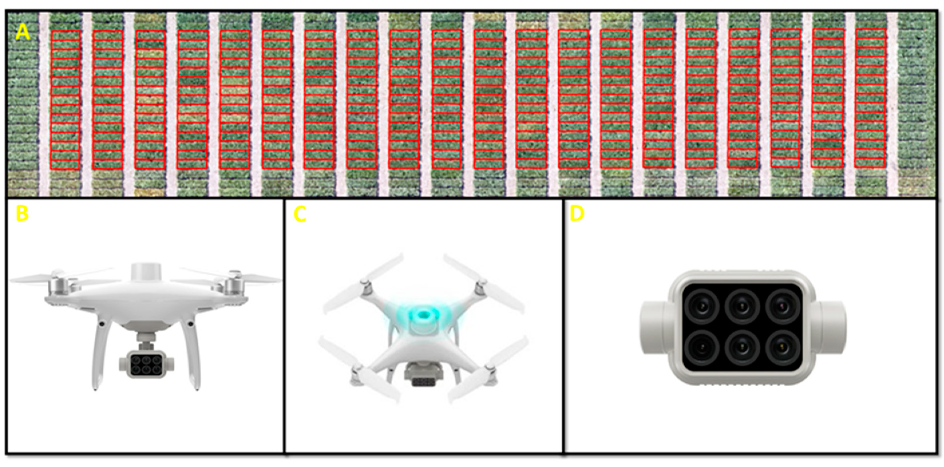
A DJI P4 Multispectral (DJI Corporation, Shenzhen, China) was the primary aerial platform to collect the remotely sensed data from the in-standing crop. The UAV was equipped with a multispectral sensor that can capture five discrete spectral bands (blue, red, green, red edge, and near infrared). Connected to the sensor was a sunlight irradiance sensor that records the dowelling radiance from the solar illumination and subsequently converts the radiance to reflectance values in a real-time manner, regardless of variations in ambient light during the collection window (Figure 2). In exchange for a very fine spatial resolution of imagery data, we programmed the UAV to fly at as low an altitude as 20 m from the surface and eventually received 1.04 cm per pixel. The low-altitude but high-resolution option necessitated the separation of the flight plan to 2 consecutive missions in the same day to fully cover the entire field. The first lengthwise flight mission covered the first column to the 15th column, which collected 300 plots, and the second covered 400 plots from the 16th column to 35th column.
To surveil the crop periodically, the aerial data collection was designed to meet the temporal dimension by flying the UAV 5 times throughout the growing stages, from the first flight on 30 August 2021 (tillering) until the last flight on 17 November 2021 (flowering). Table 1 summarizes the collection campaigns for both UAV remote sensing and ground truth data and corresponding growing stages.
The post-collection process for the UAV aerial data entailed the practice of geo-referencing and ortho-mosaicking snapshot images to a geo-corrected ortho-image of the entire wheat field. With the assistance of the real-time irradiance sensor mounted upward on the UAV and the availability of the auto-conversion of radiance to reflectance function, the imagery data could output the reflectance values without interference. Pix4D mapper software (Pix4D SA, Lausanne, Switzerland) allowed mosaicking and rectifying of the airborne multispectral images. ArcGIS Pro 3.0 (ESRI, Redlands, CA, USA) enabled georeferencing the field ortho-images and ensured that each image of a collection date plot-wise precisely overlaid the ones of the consecutive dates, which created a spatial-spectral-temporal data cube.

2.3. Ground Data Collection

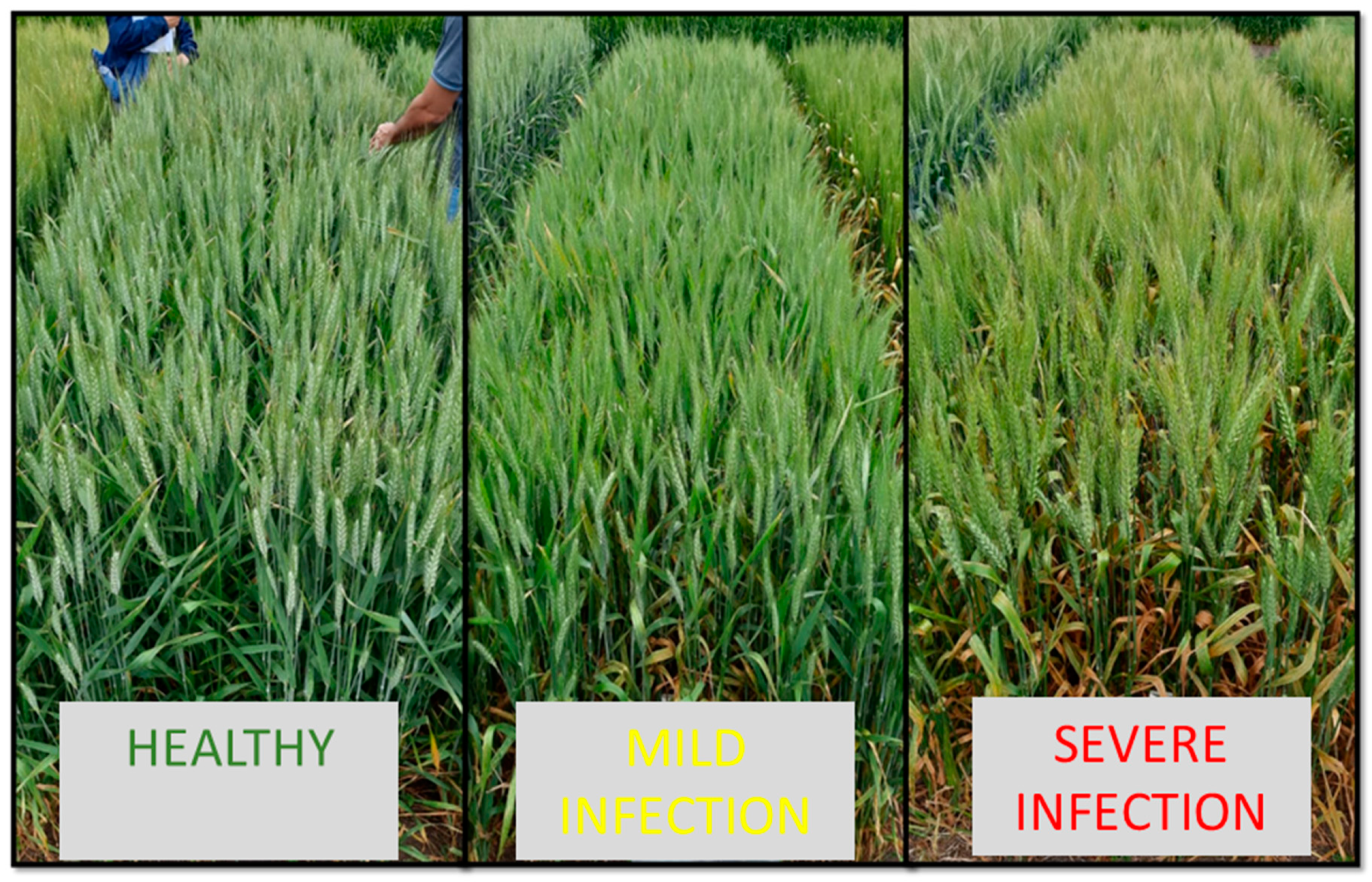
A team of pathological and phenological specialists headed to the experiment site on November 15th to visually assess the health status of the wheat and annotate them into categories of healthy, mild disease, and severe disease (Figure 3). The specialists judged the status of disease infection by spotting damage on the leaves of the plants in each plot. If the plants’ leaves had no loss in green, the whole plot was labeled as healthy. If several yellow spots existed, it was labeled as mild infection, and as severe infection if almost all plants in the plots were yellowish. It was noted that the crop health status annotation was restricted to 592 out of 700 plots due to a constraint on labor availability.
The grain yield data of the 700 plots were collected plot-by-plot at the end of growing season by an Almaco harvester, which is specialized for harvesting with breeding purposes. After the wheat in each plot was cut down, the seeds of each plot were taken into the breeding station where they were sorted and weighed. A correction for humidity in the grain composition was made to ensure standardization and compatibility. The measures were finally extrapolated from kg/plot to kg/hectares.

3. Method

3.1. Descriptive Statistics

The wheat field had 700 plots in total, among which 592 plots were disease-annotated and 108 plots were of unknown health status. The statistics of harvest yield (Table 2) on the 700-sample dataset and 592-sample subset appeared to be almost identical across the metrics, which implied the possibility of a result generalization from the smaller to the larger set. Within the 592 plots, the pathologists categorized 106 healthy plots, 430 mild infection plots, and 56 severe infection plots. A glimpse into the mean values among three groups showed a subtle difference between the healthy and mild infection groups, while the severe infection group seemed to have a lower mean yield than other two groups. An in-depth analysis was carried out and is presented in the next sections.

3.2. Feature Engineering for Machine Learning

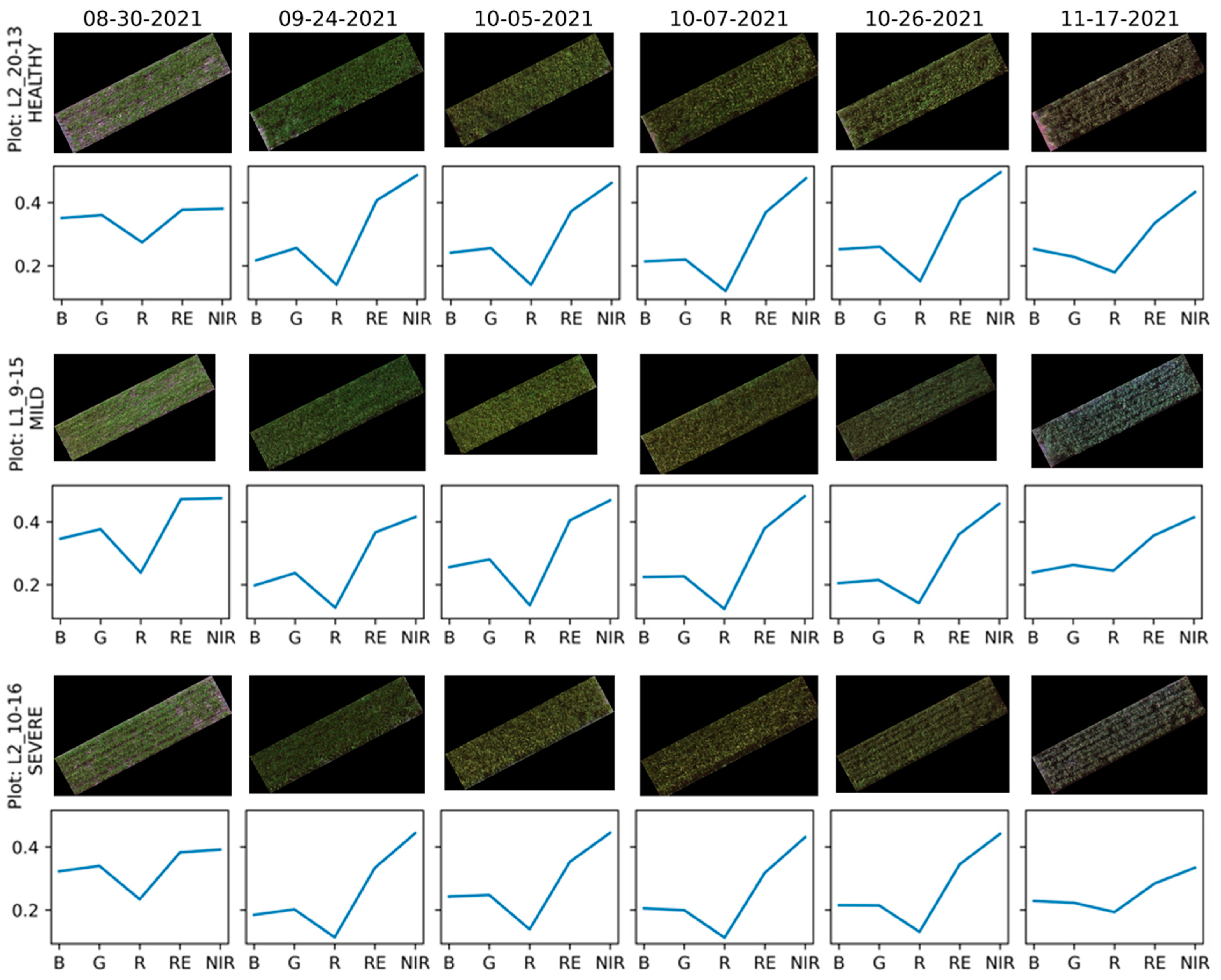
By overlying plot boundary vectors on the field ortho-image, image chips of plots were individually cropped, along with attached information of plot identification and disease labels. Figure 4 displays a drone’s-eye view of each plot in each healthy standing category: healthy, mild infection, and severe infection, as well as the corresponding spectral profiles of each plot over time. It is vital to select and transform input features, converting them from raw to amenable to a predictive model using machine learning. The process becomes more necessary when the input data is a high-dimensional imagery type that can decompose to thousands of features of spatial, spectral, and temporal dimensions, and, if improperly engineered, unrelated and noisy features could eventually add to the model and impede the model generalization. Isolating key spectral information, highlighting reflected vegetation patterns, and bringing in phenological domain expertise to assemble vegetation indices (VIs) is a usual practice of the vegetation remote sensing community. The very thorough review of previous articles in the section above suggested a set of 43 common VIs that could be extracted from aerial multispectral images (Table 3). The resultant plot-wise VIs had values in different scales, which required a re-scaling before being funneled to a machine learning pipeline described in the next section.
If vegetation indices (VIs) could presumably apprehend spectral details from the UAV multispectral images, texture features is another level of information that measures the spatial variation of image grayscale levels (i.e., a single spectral band) as a function of pixel value scale. [71] brought out the concept of grayscale level of a co-occurrence matrix (GLCM) to calculate texture details, which has since become a widely used feature extraction method (Table 4). The matrix is a function of both the angular relationship and the distance between two neighboring pixels. The suggested implementation considered four angular directions (0°, 45°, 90°, 135°) between neighboring cells in the single-band image that are separated by a distance, d (1, 3, 5 in this study). These angles and distance values were then input into six second-order texture metrics in GLCM: Contrast, Dissimilarity, Homogeneity, Angular Second Moment (ASM), Energy, and Correlation, for each of the five spectral bands (Blue, Green, Red, Red-Edge, and NIR) and eventually generated 360 texture features.

3.3. A Machine Learning Pipeline

An end-to-end machine learning construct orchestrates the flow of data into, and output from, a set of multiple machine learning algorithms, which helps to streamline and automate the workflows. A sequential series of tasks in the pipeline included data scaling, data dimensional reduction, model selection, and prediction generation. As stated above, the established VIs and texture features ranged in different scales and far from each other, which could confuse the learning algorithms and make the models biased toward features that have values higher in magnitude. In gradient descent-based models such as neural networks, the varying feature scales could impede the flow of gradient descent smoothly and hardly reach the minima of the loss function. Two common standard and min-max feature scalers were plugged into the pipeline as alternatives for each task. Next, principal component analysis (PCA and its kernel variants) functioned as a dimensional reduction tool because the section above brought out a total of 403 features from 43 VIs and 360 texture attributes.
The most common supervised machine learning algorithms—support vector machine (SVM) [72], random forest (RF) [73], and multi-layer perceptron (MLP) [74,75]—were selected for the pipeline. The idea of SVM under the hood is that the algorithm can create a line or hyperplane which separates the data into classes. The objective of SVM is to maximize the distance (a.k.a. the margin) between the line and the points (a.k.a. support vectors) closest to the line from classes. A number of SVM’s hyperparameters were passed through the pipeline to fine-tune and attain an optimal model, including the C parameter (controls the width of the margin), kernel function (projects original features to into a higher-dimensional space via a mapping function), y parameter (controls the distance of a single training example’s influence). RF is an ensemble learning algorithm that combines a great number of base learners (i.e., a decision tree) to achieve a better performance than each individual learner alone. Several of RF’s tunable hyperparameters were taken into the pipeline, namely the number of decision trees (k), the maximum depth that a tree can grow, and the minimum number of samples at the leaf nodes. The meta-learner RF also provided insights on the importance of a feature to the prediction power via the mean decrease impurity (MDI) analysis, which will be discussed in a later section. The MLP is a neural network constructed by input and output layers, and one or more hidden layers with many neurons stacked together. MLP relies on the feedforward and backpropagation learning mechanism to iteratively adjust the weights in the network with the goal of minimizing the loss function. A suite of hyperparameters needed tuning for the MLP including the number of hidden layers, number of neurons in each hidden layer, activation functions for each hidden layer, solver for weight optimization [76], learning rate schedule for weight updates, size of minibatches for stochastic optimizers, and number of iterations. Further, class weights were computed to offset the imbalance in the number of samples in each disease status. Lastly, a GridSearch Python library assisted to combine different sets of hyperparameters to search for an optimal pipeline, with a recommendation of at least 5-fold inner cross-validation [77].

3.4. Deep Convolutional Neural Networks

The convolutional neural network (CNN) enjoys its popularity in computer vision applications due to its efficient and robust learning process on imagery data. Compared with fully connected neural network (FCN) types such as the MLP above, CNNs have a substantially smaller number of weights in the network, largely relying on two important schemes: sparse connectivity (a single element in the feature map is connected to only a small patch of pixels) and parameter-sharing (the same weights are used for different patches of the input image). From the review above, the 3D convolutional version proved to be versatile for processing aerial remotely sensed images such as multispectral and hyperspectral. The model architecture assembled 3D convolutional and subsampling layers into a network that merits its automation and effectiveness at extracting jointly spatial, spectral, and temporal representations encoded in adjacent pixels and spectral wavelengths in the continuum of multispectral images. The first three convolutional layers were arranged with a 3D kernel cube of 5 × 5 × 3, a stride of 1 pixel, and the number of filters starting from 32 in the first layers and raising to a power of 2 in the next layers. On these particular data, the features tended to encode patterns over different tiles of a feature map, and thus the 3D maximal subsampling layers apparently obtained more informative and useful details than other pooling forms. The max pool kernel (2 × 2 × 1 in this study) could also sustain with image noise while generating features due to the quality of local invariance [35]. Inserted between the convolutional hidden layers was a batch normalization [78], which normalizes outputs from the preceding layer before passing them on as the input of the succeeding layer. The normalization over mini-batches also makes weights easier to initialize and thus increase the speed of training cycles. The execution of the prediction task was carried out by a block of two fully connected layers with 128 neuron units to map convolutional features to the output classes. The graphical illustration for the custom 3D-CNN for disease status identification was sketched in Figure 5.
A variety of well-established techniques to stabilize the network and reduce the risk of model overfitting were implemented. The usage of the Glorot uniform distribution [75] was for kernel weight initialization, while kernel bias was typically initialized with 0. The rectified linear unit (ReLU) [79] is well-known for countering the vanishing gradient problem when adding more layers to the network. The regularization scheme to prevent model overfitting included dropout [80] and elastic net [81]. The former involves the removal of random filters of convolutional layers in each cycle of training to reduce the possibility of model overreliance on certain features. The latter is a network regularization combined by L1 and L2 regularizers together to elevate the shortcomings of the individual techniques by reducing the impact of different features while not eliminating all of the features. The Adam (adaptive moment estimation) optimizer assisted in finding the global minima owing to the capability of updating step size derived from the running average of gradient moments. A dynamic learning rate scheme was set to exponentially reduce every 5 epochs as it reached closer to the minima. Lastly, data augmentation to the deep learning model was achieved by iterating random cropping within a boundary of each plot via a spatial fixed-size window [35]. With this technique, we oversampled the healthy and severe classes to be nearly equal to the number of samples in the majority class, mild infection.

3.5. Model Evaluation and Assessment of Disease Impact on Yield Loss

It is essential to test the performance of prediction algorithms on independent and unseen samples, and we therefore randomly split the dataset by a ratio of 60%-20%-20% for training, validation, and testing. The model performance on the holdout test set laid a basis for model comparison across algorithms and datasets. The disease status results were computed and represented on a confusion matrix, which could later derive quantitative metrics used to report the accuracy. Overall accuracy (OA) measures the number of correctly classified samples to the total number of test samples. Dealing with imbalanced data in the study, the F1 score could express a better view on the model accuracy. Lastly, we also reported the accuracy of each disease status and their meanings to the practicality.
OA = ( T P + T N ) ( T P + T N + F P + F N )
F 1   score = 2 T P 2 T P + F P + F N
Accuracy   i   class = T P i T P i + F N i
where True Positive (TP) and True Negative (TN) are the number of plots for a disease status correctly predicted by the model, and False Negative (FN) and False Positive (FP) are the number of plots for a certain status wrongly predicted as another status.

4. Results

4.1. Temporal and Spectral Dimensions by Disease Status

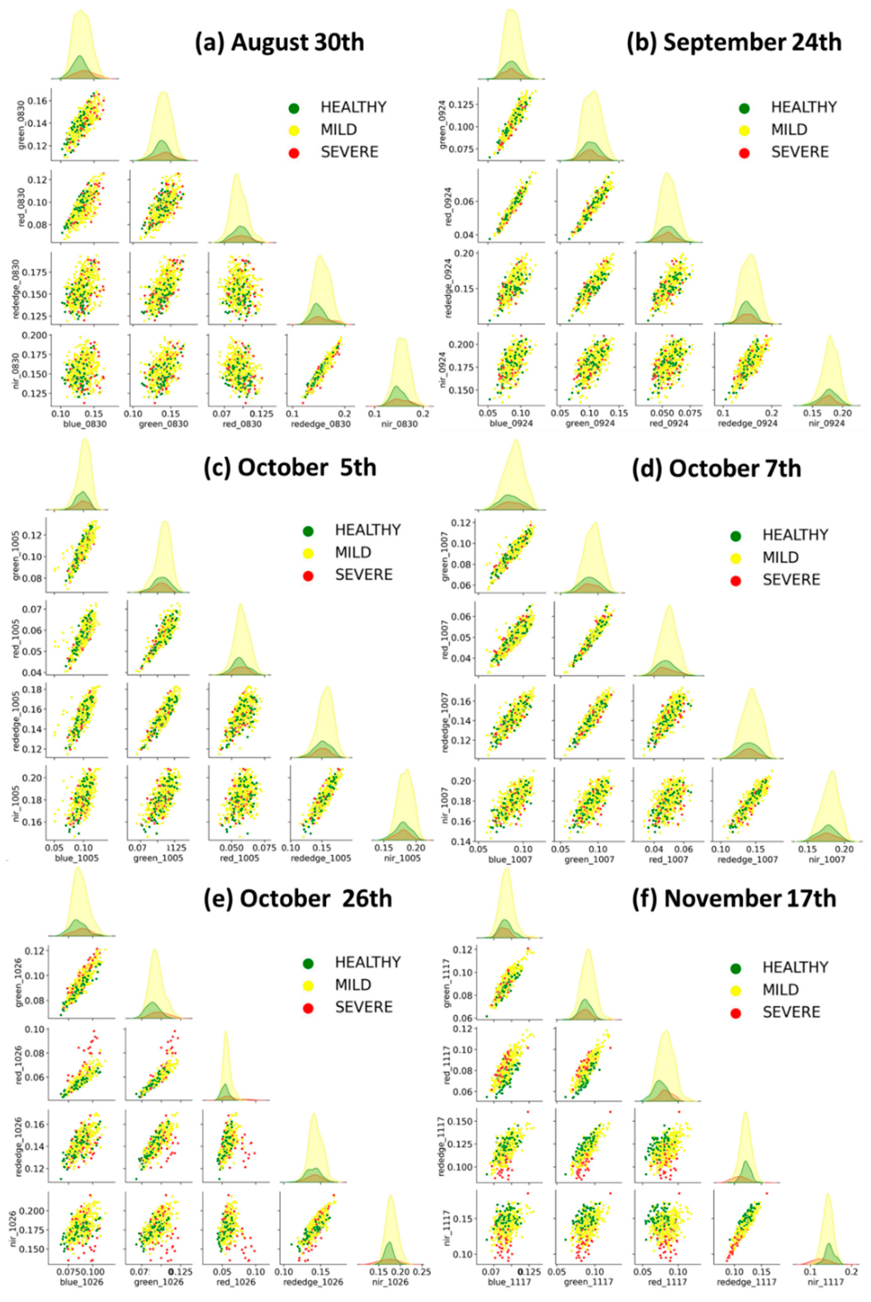
It is worthwhile to provide exploratory insights of yellow rust progress by original spectral bands along the temporal dimension (Figure 6). With only five original spectral bands, the wheat health categories could be seemingly indistinguishable early in the crop’s life course. The juxtaposed histograms of healthy, mild, and severe categories in Figure 6a–d’s diagonal axes confirmed an undivided state. Progressing until 98 days after sowing (DAS) (Figure 6e) and thereafter (Figure 6f), the severe infection was plainly discernible by the red-edge and NIR bands. The separation of healthy and mild infection appeared to be impossible over the course of time.

4.2. Dimensional Reduction by Principal Component Analysis

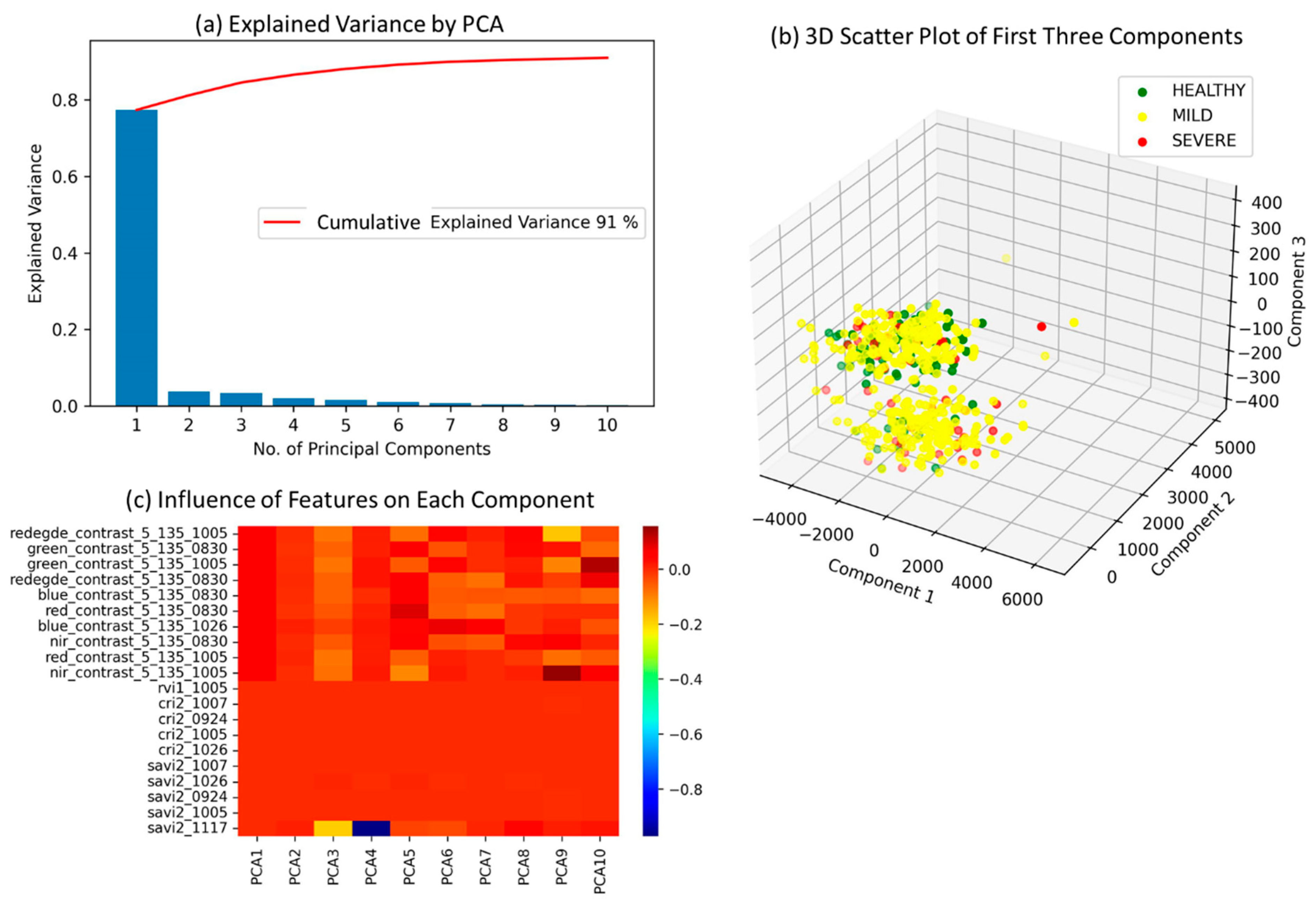
It became obvious that the contributory value of five raw spectral bands toward a highly accurate disease identification was insufficient, which explains the addition of 43 common VIs and 360 texture attributes to improve the prediction accuracy. Figure 7 elucidates the result of dimension-reduction principal component analysis (PCA) in reducing the combined data of five spectral bands, 43 VIs, 360 texture attributes, and their temporal values of six collection dates from 2448 features to 10 features. It is noted that with an assistance of GridSearch Python library, we experimented with a wide range of a reduced number of components and came up with the best parameter at 10 features (Figure 7a) that cumulatively explained 91% of the variance of the original data. The first three PCA components (Figure 7b) revealed a definite opportunity to separate healthy (green dots) and severe infection plots (red dots). The influence of each feature on the PCA components can be partially viewed from Figure 7c. Among the 10 most positive correlations with PCA components, the texture contrast with a distance of 5 and an angle of 135° in all spectral bands at the early time had the most positive relationship with the PCA components. Conversely, at the later stages, the vegetation indices such as SAVI2 and CRI2 were among the 10 most negatively related to the PCA components. It bears noting that the sign of correlation coefficients was not a matter, but the higher magnitude of the coefficients between the texture features and the first PCA component (Figure 7c, dark red) indicated a greater influence of texture features than VIs (Figure 7c, light red).

4.3. Classification Performance of Fused Data and Classifiers

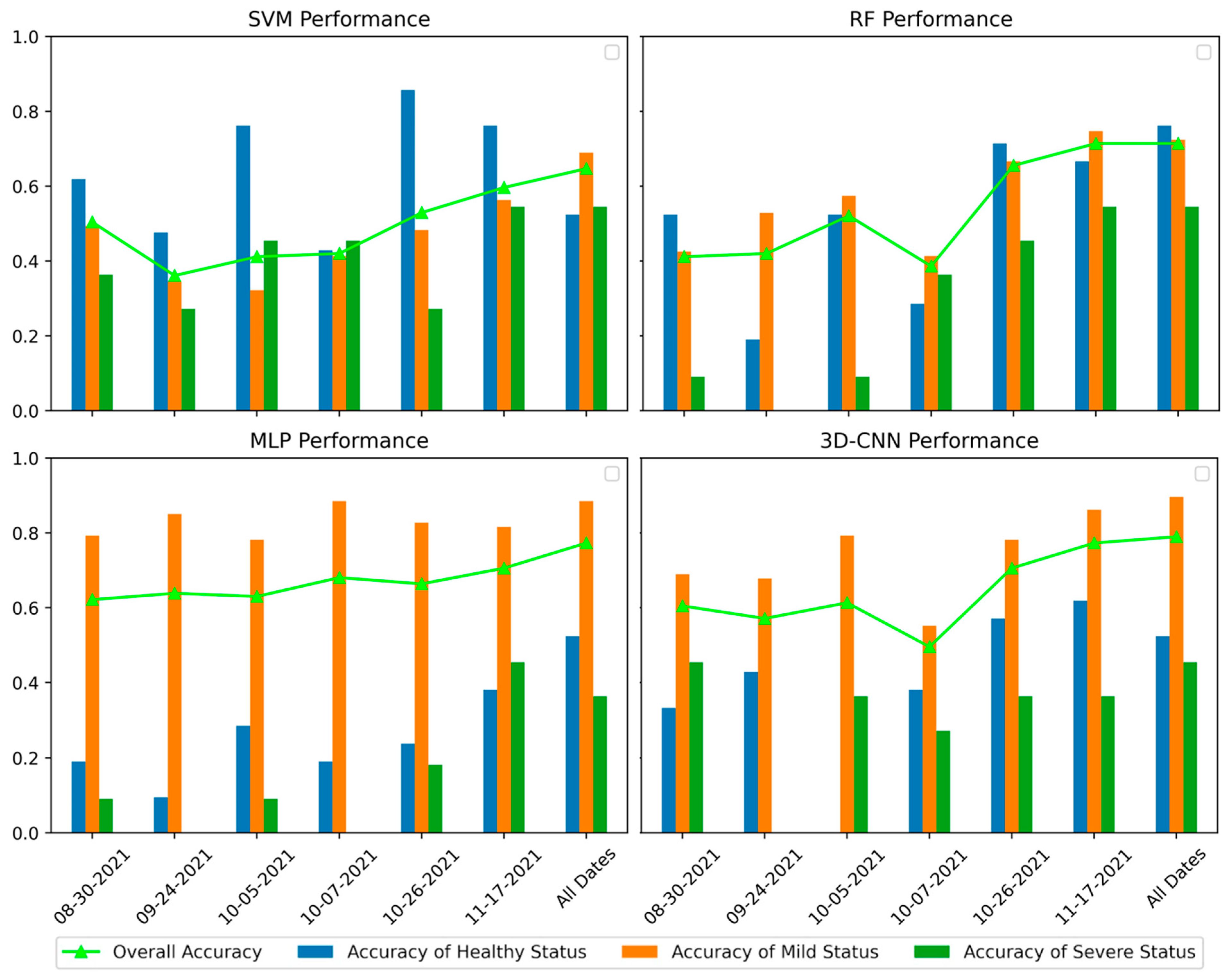
The four machine learning classifiers resulted in different performance of disease status identification on the spring wheat (Figure 8). At first glance, the resulting overall accuracy (OA) varied from model to model, but increased along the temporal dimension. With the earliest UAV aerial images on August 30th, the best model 3D-CNN could detect the wheat’s health standing at the OA = 60%. As the season went on, the OA of the 3D-CNN improved to 77% on the November 17th dataset. The temporal fusion of datasets apparently became superior in the OA, with 65%, 71%, 77%, and 79%, respectively, as results from the SVM, RF, MLP, and 3D-CNN. The RF and 3D-CNN handled the imbalance class issue better than the SVM and MLP when the results from both SVM and MLP favored a certain class (i.e., the healthy plots and mild infection plots, respectively).
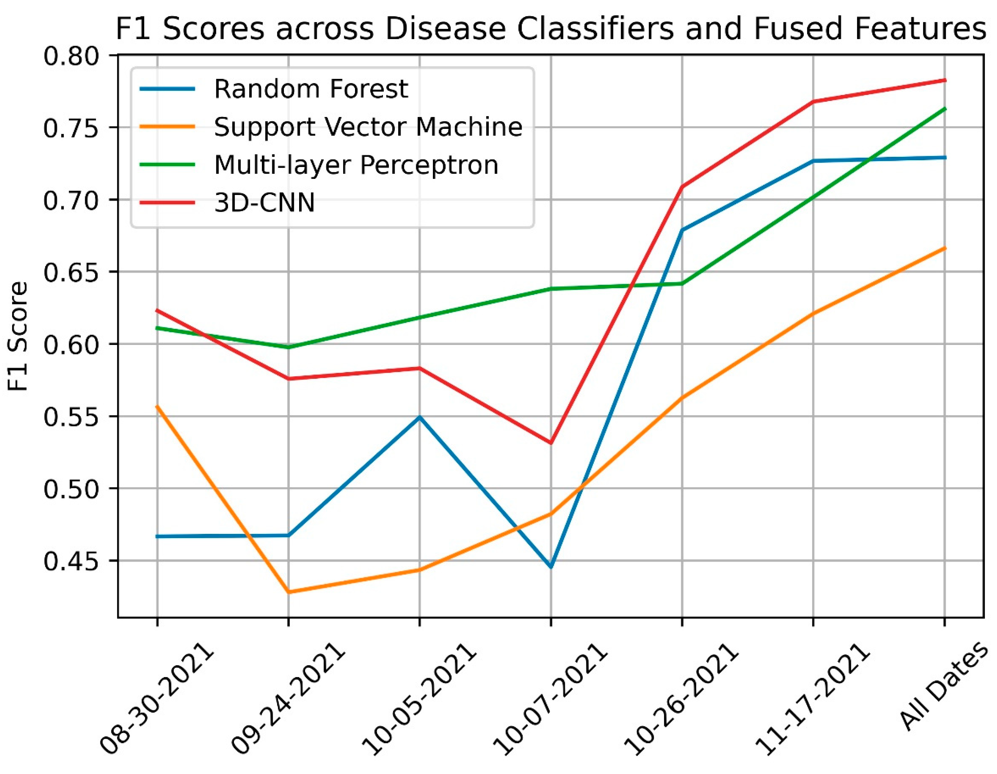
The OA and accuracy of the individual classes above could be somewhat misinterpreted by the imbalance class issue. Instead, F1 metrics are obviously a more precise and interpretable measure, which shows in Figure 9. The MLP stood out as the best prediction model for early aerial sensed images, while the 3D-CNN worked best with late-season images. The F1 score of the 3D-CNN climbed up from 0.55 in the October data to 0.77 in the November data and 0.79 in the combined data. The two classical machine learning algorithms, SVM and RF, appeared to be less able to detect yellow rust disease in the early growing season (e.g., F1 score = 0.4 by SVM prediction on September data).

4.4. Spatial Mapping of Disease Status

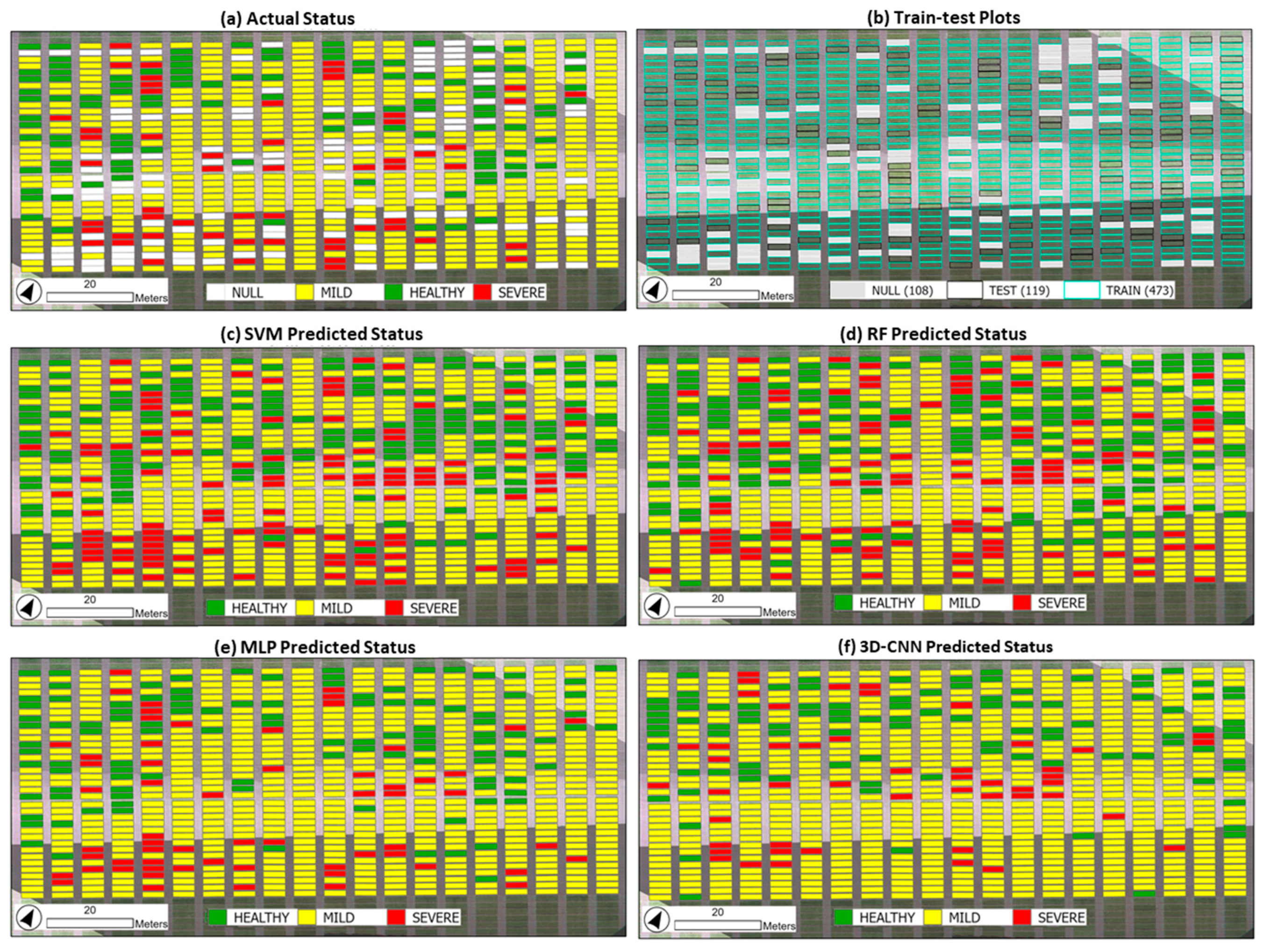
If the numerical OA and F1 metrics in the above section were derived in the test set to precisely reflect the detective performance of each algorithm, in this section we projected the best trained models of temporal-spectral-texture fused data over the entire field via spatial maps (Figure 10). Figure 10a visualizes an actual annotation of disease statuses, where mildly infected plots took the majority of the field. The yellow rust disease aggressively progressed in the bottom half of the field, or in the southeast part of the cardinal direction. In the meantime, most of the upper wheat plots (the northwest portion) were able to remain free from the disease attack. The disease developed severely in adjacent plots, but those severely attacked plots seemed to be spatially disconnected and scattered away. The machine learning algorithms on training plots (Figure 10b) were deployed on the whole field and projected the predicted disease statuses back to the map. The SVM and RF (Figure 10c,d) appeared to bias the disease detection as the two methods favored more healthy plots. Generally, this false negative type could pose a greater risk as disease-infected plots were diagnosed as healthy plots, which might lead to more disease transmission to the whole field. The MLP and 3D-CNN’s prediction (Figure 10e,f) came to more closely approach the actual patterns, which exactly located a greater number of healthy plots in the northwest area and disease plots in the opposite direction.

4.5. Spatial Assessment of Disease Impact on Yield Loss

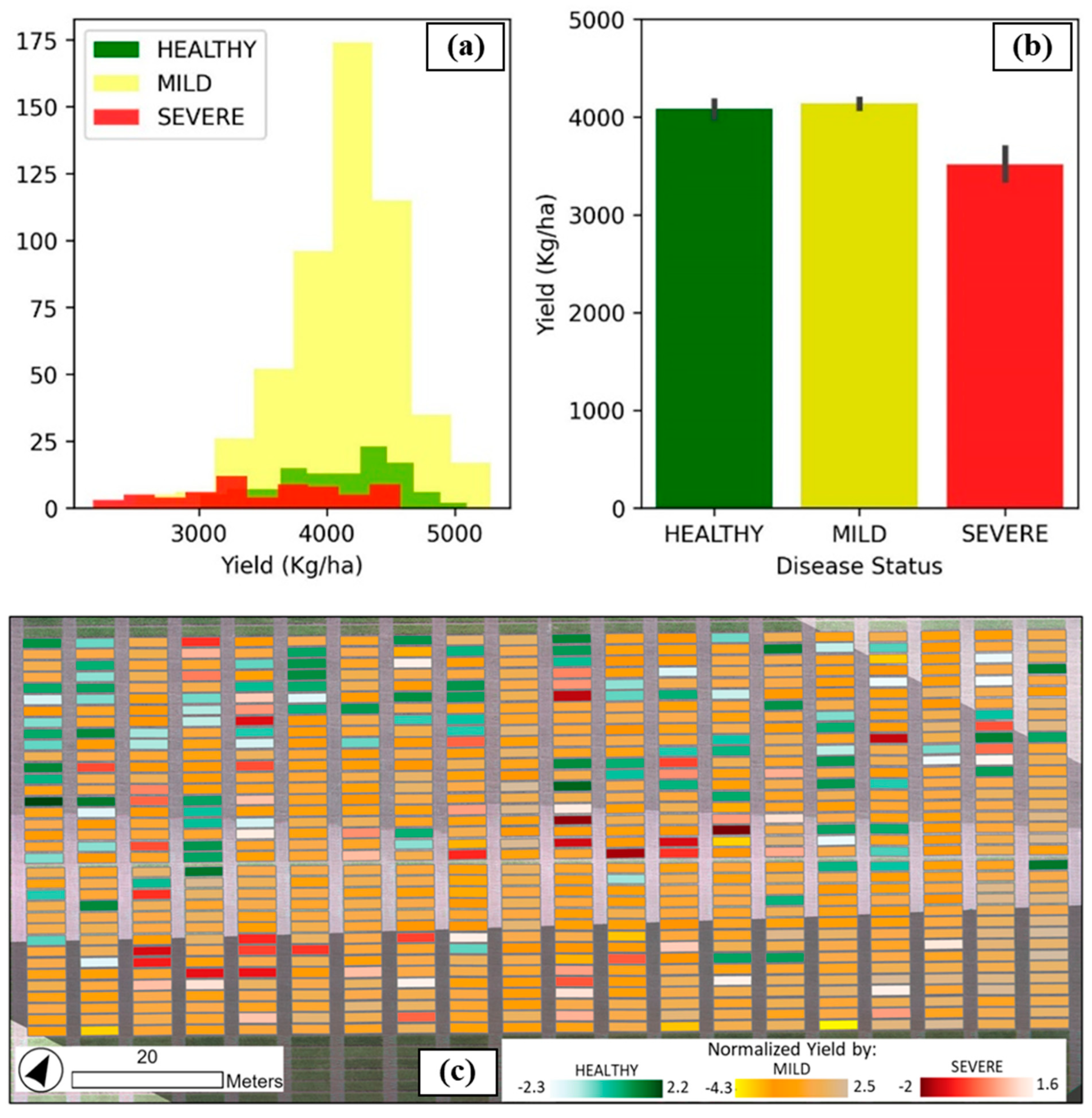
Assuming all other genetic and environmental factors held constant, the yellow rust disease obviously exerted a great influence on the variance of the end-season wheat harvest. Figure 11 demonstrates the adverse impact of the disease on wheat yield through a lens of a comparison of yield among healthy, mild infection, and severe infection. The majority of the field’s plots were mildly rust-infected (Figure 11a), and the yield harvested in these mildly-infected plots exhibited a low standard deviation and clustered values around the mean in a thin bell-shaped curve. More noticeably, the mean difference in yield between healthy and mild infection plots (Figure 11b) was very subtle, possibly gaining 4000 kg/ha on average when the season ended. The substantial loss of 500 kg/ha in the yield return could be estimated in the plots attacked severely by the disease. The normalized yield of each group centered their data to 0 with a standard deviation of 1 (Figure 11c), indicating a minimal impact of the mild rust infection on the harvesting yield, as evidenced by a few plots in the southeastern area (Figure 11c, yellow-colored plots) having yield loss. By contrast, the very low yield values were obviously found in severe infection plots, which clustered in the middle and southern part of the field (Figure 11c, dark-red-colored plots).
A one-way ANOVA hypothesis test was conducted to solidify the findings above. Table 5 summarizes the ANOVA results, comparing the means of yield produced by plots from three independent categories of wheat heath. The omnibus F-statistic = 43.92, p < 0.001 indicated a statistically significant difference overall between all groups. A post hoc Tukey’s Honest Significant Difference (HSD) [82] test was followed up to explore which pairwise comparisons were truly significantly different. As a result, the test rejected the difference in the yield harvested from healthy and mild infection plots (p = 0.2785) but accepted the difference in yield harvested from either of the healthy or mild infection plots and the severe infection plots. The test’s result also implied that in comparison with healthy wheat, a severe attack of yellow rust can erode 563.65 Kg/ha from each plot on average. The 95% confidence interval (CI) affirmed the yield loss from a severe infection could be somewhere between 375.93 kg/ha and 751.37 kg/ha.
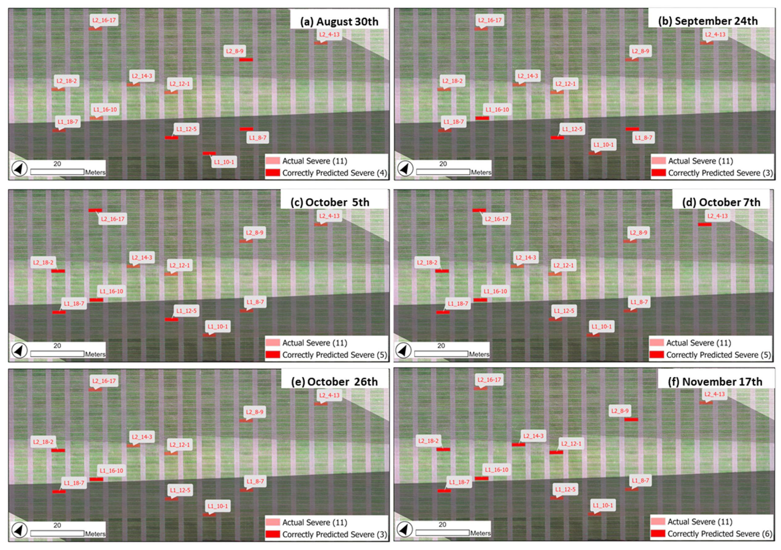
The test above firstly revealed a statistical indifference in wheat yield between healthy and mild infection plots. The fact is that the abiotic stress is not a deciding factor affecting potential yield, but other contributing factors could be considered, such as environmental conditions, or, more importantly, genotypes, not to mention the interaction between them. Plots were grown with different genotypes, among which some genotypes were highly susceptible to the rust and some were very resistant. However, the genetic information was proprietary to the data provider, and therefore we counted the factor as a limitation. The test secondly affirmed the detrimental impact of severe yellow rust attack on the harvesting yield. From this angle, correctly identifying the likelihood of a plot being severely infected by yellow rust appeared to be more critical than predicting all the classes at a high overall accuracy in determining the exact time for intervention. Both OA and F1 score (Figure 8 and Figure 9) favored the results of the 3D-CNN method at a higher accuracy, though the SVM method (Figure 8) correctly detected a greater number of severe infection plots than the 3D-CNN did. Figure 12 spatially presents 11 plots annotated as severe infection in the test set (119 plots) and the associated SVM predictions over different stages of the crop’s growing season. The probability of correctly detecting a severe attack of yellow rust increased from 36.37% (4 out of 11 plots) on 30 August (40 days after sowing) to 54.54% (6 out of 11 plots) on 17 November (121 days after sowing). Upon the detection, an implication that can translate the disease probability to potential yield preservation could be simply carried out to help the crop growers. This will be inclusively discussed in the next section.

5. Discussion

5.1. Importance of Spectral, Texture, and Temporal Information

The results above to some extent highlighted the significance of each dimension of information used in the study. The multispectral images with recorded information at five discrete wavelengths apparently offered a greater chance than regular RGB images to detect changes in crop’s defenses when they were fighting against foreign invaders. The red-edge (RE) (690–740 nm) and NIR (740–1000 nm) spectral bands (Figure 6) proved to be key indicators of distinguishing rust-infected plots from the healthy. This finding was somewhat aligned with what [4,6] found in their studies, in that the NIR band brought the most discriminating power to classify wheat disease severity. It is plausible that the presence of yellow rust in wheats led to a decrease in RE and NIR reflectance, and, more importantly, the amount of the decrease was proportional to severity levels of infection as a function of time. This is mainly because of a reduction of chlorophyll content and an increased evaporation on the stressed wheat leaves that made them turn brown and dry, which can also be effectively sensed by low altitude UAVs at a canopy level. More concretely, the finding was also supported by the feature importance analysis (Figure 7c), which revealed the two most influential VIs, the carotenoid reflectance index 2 (CRI2) [70] and soil-adjusted vegetation index 2 (SAVI2) [48]. The former index was arithmetically formed from the green and RE bands, while the latter was derived from the red and NIR bands.
The grey-level co-occurrence matrix (GLCM) texture features named the image contrast as the most sensitive to PCA components when predicting disease statuses (Figure 7c). The contrast feature measures the difference between the highest and the lowest values of the adjacent sets of pixels of a certain spectral band. The discriminating power of the image contrast occurred in all five spectral bands but particularly in airborne multispectral images collected at the early stage of infection from 40 DAS to 77 DAS. Studies [21,22] utilizing hyperspectral images for yellow rust monitoring also highlighted the predictive capability of the image contrast feature. However, their findings occurred only in late infection stages, which was then explained by very minimal external characteristics obtained during asymptomatic or mild infection; instead, the majority of alterations resided in pigment-related inner tissues of plants which were more properly accessible through VIs than texture features. Owing to a very much finer resolution of 1.04 cm per pixel, our study disclosed that the contrast texture feature extracted from early collected images could bring more value and set a higher statistical dependency on the prediction model. Conceptually, the crop’s structure, the canopy shape, and the leaf morphology of single plants could be separately obtained by the UAV without the confounding effects of neighbor plants when the plots were lower-density and higher open space. The optimal distance d at 5 pixels and angular direction θ of 135° found in this study solidified the conjecture above when the 5 pixels were equivalent to 5–6 cm, which was roughly the size of a single plant at the stage of tillering and stem elongation.
The predictability of the temporal dimension became manifest in the increased accuracy and F1 metrics (Figure 8 and Figure 9, 3D-CNN Performance). At the early onset stage when the crop was tillering (40 DAS), the aerial remotely sensed images correctly recognized the wheat’s health standing at 60% accuracy, seemingly leveling off the accuracy at 57%, 61%, and 50% at the stem extension and heading stages (65–80 DAS) before picking up the increasing pattern at a high accuracy of 71% and 77% at the later booting and flowering stages (100–120 DAS). The disease detection pattern found in this study was very consistent and identical with those in previous studies of spatio-temporal yellow rust monitoring [4,6]. There exists, however, an underpinning difference in that the previous studies purposefully and artificially inoculated the disease in wheats with several preset severity levels, whereas our experimental field was naturally invaded by the pathogens with an uncertainty of the attack severity. The natural outbreak posed a real challenge in this study, such that early season infection was supposed to be varied from plot to plot. In certain plots, the pathogen survived in wheat as dormant mycelium, while in other plots, violent infection resulted in plant stunting that reflected its vigor and shape in the UAV’s sensor. The mid-season then developed the complication of multiscale and various-speed spreading of the disease. The yellow conspicuous rows on old leaves turning brown and dry were obscured by the new green leaves emerging on the top of the canopy (Figure 3) where the UAV flew over for a nadir-angle data capture. The later flowering stage, though, somewhat negated the detectability, confusing whether a reduced greenness in a certain area was caused by the disease or the emergence of the wheat spikes. This stage also witnessed the infection reaching maturity and violently and uniformly spreading over all of the plots, which wholly lost the greenness and made it easier for the aerial surveillance.

5.2. Prediction Performance of Multimodality Fusion

With the values of each dimension discussed earlier, the inclusion of these information dimensions together was obviously worthwhile. An improved accuracy of combined-data models could be observed across all the machine learning algorithms SVM, RF, MLP, and 3D-CNN, at 65%, 71%, 77%, and 79% respectively (Figure 8), which was considerably higher than any single-data models. Not only research on wheat yellow rust control [4,6,21,22], but also various remote sensing applications, such as grapevine viral disease detection [9], soybean yield estimation from the aerial scale [83] or satellite observation [34], urban tree classification [84,85], and maize high-throughput phenotyping [35] demonstrated a 3–10% improvement if a fusion of different modalities were applied. Apparently, in as many representations of the crop as being sensed, each of these, either singly or jointly, supplemented the predictive power to detect the crop’s disease severity. More specifically, spectral bands and VI derivatives characterized ample information related to leaf and stem pigments, leaf biochemicals (e.g., protein, lignin, cellulose,…), cell structure, and water content [9,86]. GLCM texture features communicated spatial variations of crop vigor and structures, i.e., leaf and canopy shapes [87,88]. Temporal data provided insights of crop growth characteristics, health status, and the infection progress as a function of time. The benefit of the aggregated insights was more than proportional because each time the UAV flew over a certain plot, it collected different and new details of that particular plot when plots were geo-referenced.

5.3. Comparison between Traditional Machine Learning and Deep Learning 3D CNN

The predictive performance comparison was shown in Figure 8 and Figure 9 (accuracy metrics and F1 scores) between feature-wise and image-wise methods, or, more precisely, between traditional machine learning and deep learning CNN’s 3D version. The F1 prediction metrics favored the deep learning method over the other three classical machine learning methods, with the exception of the September and early October datasets. The MLP produced a higher F1 score but failed to solve the class imbalance issue, leading to higher accuracy of the mild infection class, but very low accuracy of the healthy and severe infection classes. Most of the findings from various studies [9,28,33,35] have also advocated for the CNN, perhaps for the several following reasons. First, the assembling of multiple filters and 3D kernel cubes with a sliding window size of 5 × 5 × 3 lent the CNN itself to effectively gather all possible information from each wheat plot. Most especially, at the sliding step of 1 unit, the 3D kernels can powerfully uptake and retain interrelated and interdependent spatial-spectral features prior funneling the learned features to the prediction layers at the end of the network. Concrete evidence could be visibly viewed through a higher accurate prediction of the 3D-CNN for the 30 August data, when the field plots contained a mixture of vegetation and soil objects. With the feature-fed machine learning method, the input features had been confounded by the soil and non-vegetation features, not to mention the fact that the separate extraction of spectral bands, VI, or texture features possibly suggested an inadequate capture of mutually spectral-spatial-temporal information on wheats. Second, the infection progressed and spread heterogeneously within a plot, meaning some plants were infected while the others remained green and healthy. The data augmentation applied in the study by repetitively and randomly cropping image chips in all areas of a plot essentially enriched crop plots’ information more than simply taking average values of plots. Third, the working mechanism of automated feature learning in the image-centric 3D-CNN method by a bi-directional optimization process (i.e., forward and backward propagation) [89] appeared to be more competent than feature engineering in locating and retaining discriminating representations. The handcrafting procedure heavily relied on expert knowledge and human decisions to be established, and thus, was highly likely to be susceptible to missing previously unknown but pertinent informative parameters.

5.4. Impact of Disease on Permanent Yield Loss

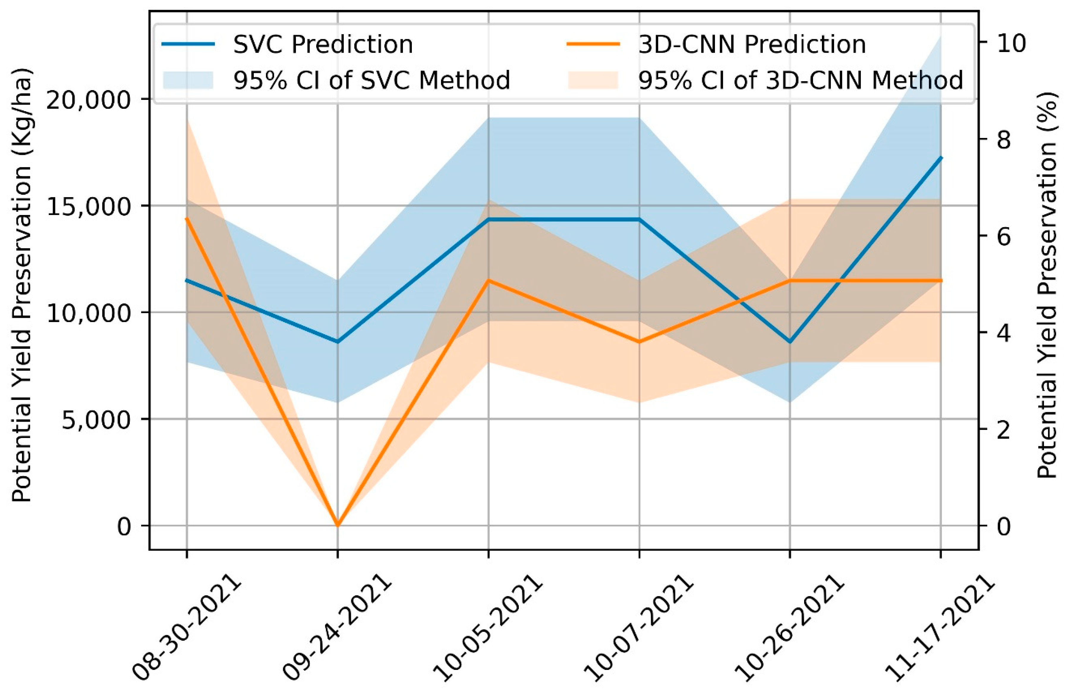
What made this study intriguing lay in the post-detection application regarding determining permanent yield loss as well as an intervention period to prevent the loss. The ANOVA test indicated a significant yield loss if a wheat plot is severely attacked by yellow rust. For this reason, a post-detection focus of identifying early only severe infection plots could be more meaningful to the farming practice. Despite a higher OA and F1 scores predicted by the 3D-CNN, the SVM turned out to be better for this specific task, detecting severe plots at a higher accuracy. It is commonly accepted that the automated feature learning process of 3D-CNN demands a sufficiently large volume of data to achieve its excellence in learning performance, but the study had a few numbers of plots annotated and labeled as severe infection (56 plots for both training and testing). Assuming a constant of genetic and environmental factors, the translation from the probability of successfully detecting severe attacks to permanent yield loss were simply achieved by multiplying the 563.65 kg/ha difference in the yield harvested between severe infection plots and control plots (healthy wheats) (Table 5). The estimated yield loss is able to be reversed to possible attainment if crop growers detect disease early and properly intervene. Figure 13 presents the absolute figures of potential yield preservation for this specific field (Figure 13, left vertical axis) and relative figures in percentage for generalization (Figure 11, right vertical axis). The earliest estimation from the SVM method could help to preserve 8000–15,000 kg/ha for this farm, which was functionally equivalent to 3–7% of the possible yield preservation in general. Similar quantities were also found in agronomical lab-based studies in different wheat varieties and conditions [90,91,92].

5.5. Limitations of UAV Aerial Data

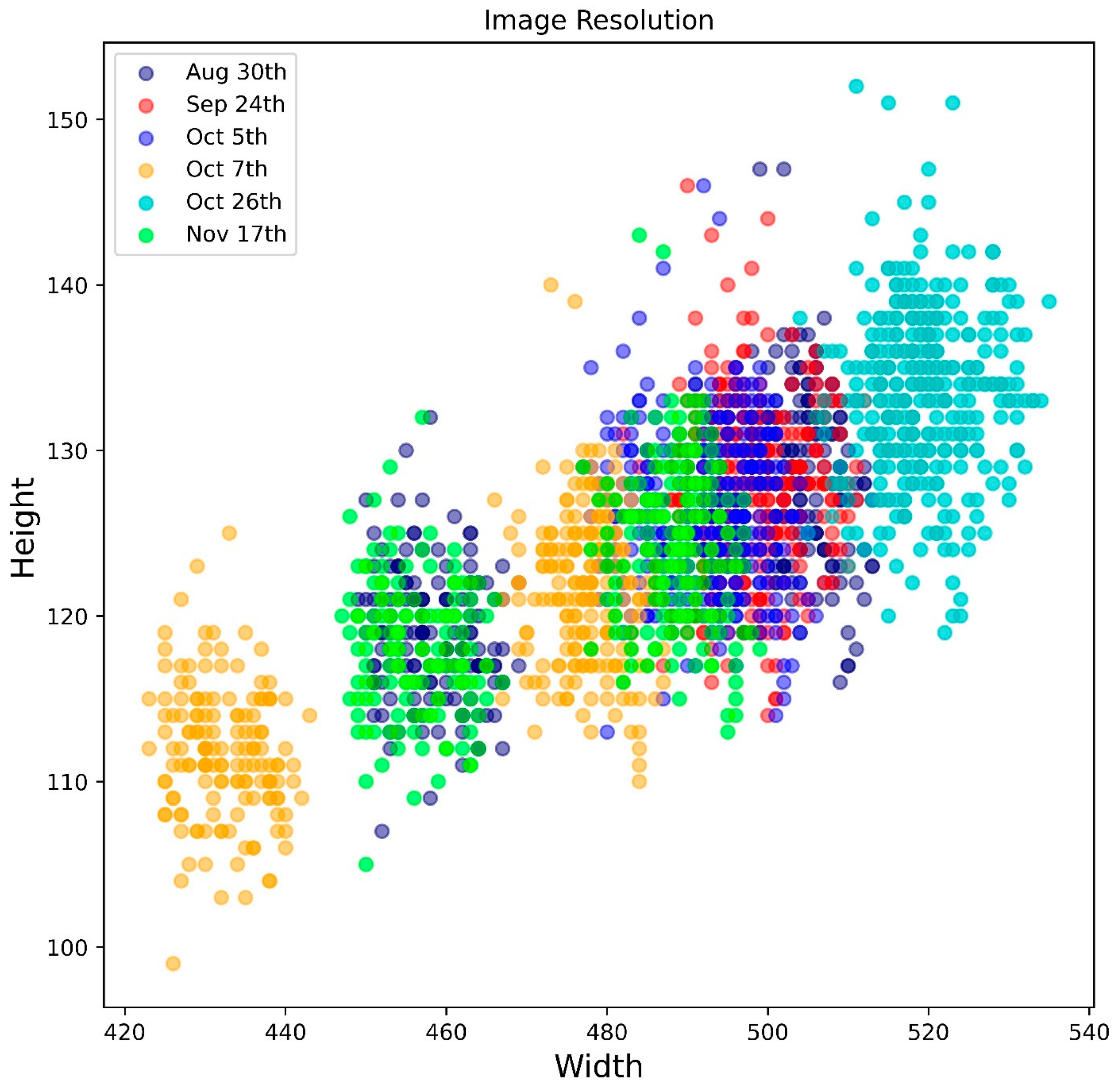
Compared to ground or proximal sensing, several noticeable challenges of aerial remote sensing for disease monitoring are the objects’ reflectance information captured in a substantially-reduced spatial resolution, in addition to meteorological effects of atmosphere and illumination variation. Further, the study incurred discrepancies in the spatial resolution of UAV aerial images (Figure 14), which in turn deteriorated some parts of the results. The very large field and constraint of battery capacity limited the UAV to conduct a single flight mission to cover the entire field. Different flight missions in the same collection date caused a discrepant spatial resolution of plot-level image chips. For instance, the image resolution of the data collected on 7 October (Figure 14, orange dots) varied between two flight missions;, more specifically, images collected from the first flight had a coarser resolution than those from from the second flight. The underlying causes could be traced back to an unreliable flight planning software, imprecise in-flight motion adaptation, in-flight GPS signal loss or interruption, etc. Several UAV studies found a similar phenomenon in their aerial data [22,93,94].
The image resolution variation probably brought a negative effect on establishing GLCM texture features and image-based CNN methods more than VI-based models because the texture or CNN calculations were typically controlled by the pixel size and the neighborhood relation of adjacent pixels. In addition, the yellow rust pathogens developed and spread out in a spatial pattern as discussed in the foregoing sections, but variation between the flight missions existed and hindered the observation, especially longitudinal disease monitoring over time. It was plausibly explained why two datasets collected from consecutive dates, 5 and 7 October, yielded considerably different accuracies. Unlike the 7 October data, all of the plot-level image chips of the 5 October data (Figure 14, blue dots) more consistently clustered in a finer resolution of 490 × 130 pixels.

6. Conclusions

The work methodically presented an automated disease monitoring system for worldwide yellow rust in wheat with an aerial remote sensing platform in combination with state-of-the-art machine learning techniques. Early detection of infectious disease is obviously a real challenge but this study evidenced a possibility that UAV airborne multispectral images can detect the disease early and disseminate actional information to crop growers in a timely manner to prevent potential yield loss. From the above findings and discussions came the following conclusions:
  • Red-edge (RE) (690–740 nm) and near infrared (NIR) (740–1000 nm) were critical spectral bands to distinguish between healthy wheats and severely yellow-rust-infected wheats. All raw spectral bands originally obtained from the UAV were incapable of differentiating healthy and mildly infected wheats.
  • Among engineered features, the carotenoid reflectance index 2 (CRI2) [70] and soil-adjusted vegetation index 2 (SAVI2) [48] became the two most influential VIs in detecting disease infection early. Similarly, GLCM contrast texture at an optimal distance of d = 5 pixels and angular direction of θ = 135° from airborne multispectral images brought in the most predictive value for disease sensing.
  • The AI-powered wheat disease monitoring performed at 60% detection accuracy as early as 40 DAS when tillering, increasing to 71% and 77% at the later booting and flowering stages (100–120 DAS). The accuracy reached a peak of 79% for the spectral-spatio-temporal fused data model.
  • Neither relying on human expertise nor being prone to human judgement, the imagery-based 3D convolutional neural network (3D-CNN) method, on the basis of an automated learning process, outperformed feature-based machine learning methods in detecting the wheat disease invasion early.
  • Violent attacks of yellow rust on wheats permanently caused a significant amount of yield loss. The success of early sensing from low-cost multispectral UAVs could preserve a potential amount of yield of 3–7% at the confidence level of 95%.
Interested readers are highly encouraged to recognize the study’s limitations and delimitations below before making any generalizations. The use of aerial observation platforms other than DJI P4 Multispectral (DJI Corporation, Shenzhen, China) with the mounted multispectral sensor could lead to a different result. At the authors’ discretion, another study, carrying the same data but different machine learning or deep learning methods, could produce a result varying from the one found in this study. This work attempted to address the small size and imbalance class issue in actual samples by technical techniques described in the forgoing sections, but they are by no means negligible limitations. Further research should collect a larger and more balanced number of observations, such that the study reliability could be assured. The longitudinal disease severity assessment by collecting disease status in multiple timestamps is highly suggested to accommodate this study limitation that overlooked the developmental infection process on each plot. There existed room for further improvement by designing an advanced deep learning architecture or leveraging the capability of transfer learning to optimally comprehend intra- and inter-related spectral-spatio-temporal patterns of disease progress. The possibility of having different wheat varieties tested in multi-location, multi-season, and multi-environment fields, in addition to multiscale remote sensing (underground, proximal, low-altitude aerial, and satellite) is highly suggested to confirm the results’ consistency, as those mentioned factors were noteworthy limitations in this study.

Author Contributions

Conceptualization, C.N. and V.S.; methodology, C.N. and V.S.; software, C.N. and V.S.; validation, C.N. and V.S.; formal analysis, C.N. and V.S.; investigation, C.N. and V.S.; resources, C.N. and V.S.; data curation, C.N., J.S. and V.S.; writing—original draft preparation, C.N.; writing—review and editing, C.N., J.S. and V.S.; visualization, C.N. and J.S.; supervision, V.S.; project administration, V.S. and J.I.S.; funding acquisition, V.S. All authors have read and agreed to the published version of the manuscript.

Funding

This work was funded by NSF CPS award (2133407) and USGS AmericaView Grant (G18AP00077).

Data Availability Statement

Not applicable.

Conflicts of Interest

The authors declare no conflict of interest.

References

  1. Yuan, L.; Huang, Y.; Loraamm, R.W.; Nie, C.; Wang, J.; Zhang, J. Spectral analysis of winter wheat leaves for detection and differentiation of diseases and insects. Field Crop. Res. 2014, 156, 199–207. [Google Scholar] [CrossRef] [Green Version]
  2. Moshou, D.; Bravo, C.; West, J.; Wahlen, S.; McCartney, A.; Ramon, H. Automatic detection of ‘yellow rust’ in wheat using reflectance measurements and neural networks. Comput. Electron. Agric. 2004, 44, 173–188. [Google Scholar] [CrossRef]
  3. Duan, T.; Chapman, S.; Guo, Y.; Zheng, B. Dynamic monitoring of NDVI in wheat agronomy and breeding trials using an unmanned aerial vehicle. Field Crop. Res. 2017, 210, 71–80. [Google Scholar] [CrossRef]
  4. Su, J.; Liu, C.; Coombes, M.; Hu, X.; Wang, C.; Xu, X.; Li, Q.; Guo, L.; Chen, W.-H. Wheat yellow rust monitoring by learning from multispectral UAV aerial imagery. Comput. Electron. Agric. 2018, 155, 157–166. [Google Scholar] [CrossRef]
  5. De Castro, A.; Ehsani, R.; Ploetz, R.; Crane, J.; Abdulridha, J. Optimum spectral and geometric parameters for early detection of laurel wilt disease in avocado. Remote Sens. Environ. 2015, 171, 33–44. [Google Scholar] [CrossRef]
  6. Su, J.; Liu, C.; Hu, X.; Xu, X.; Guo, L.; Chen, W.-H. Spatio-temporal monitoring of wheat yellow rust using UAV multispectral imagery. Comput. Electron. Agric. 2019, 167, 105035. [Google Scholar] [CrossRef]
  7. Zheng, Q.; Huang, W.; Cui, X.; Dong, Y.; Shi, Y.; Ma, H.; Liu, L. Identification of wheat yellow rust using optimal three-band spectral indices in different growth stages. Sensors 2018, 19, 35. [Google Scholar] [CrossRef] [Green Version]
  8. Chen, X. Epidemiology and control of stripe rust [Puccinia striiformis f. sp. tritici] on wheat. Can. J. Plant Pathol. 2005, 27, 314–337. [Google Scholar] [CrossRef]
  9. Nguyen, C.; Sagan, V.; Maimaitiyiming, M.; Maimaitijiang, M.; Bhadra, S.; Kwasniewski, M.T. Early detection of plant viral disease using hyperspectral imaging and deep learning. Sensors 2021, 21, 742. [Google Scholar] [CrossRef]
  10. Sankaran, S.; Mishra, A.; Maja, J.M.; Ehsani, R. Visible-near infrared spectroscopy for detection of Huanglongbing in citrus orchards. Comput. Electron. Agric. 2011, 77, 127–134. [Google Scholar] [CrossRef]
  11. Devadas, R.; Lamb, D.; Simpfendorfer, S.; Backhouse, D. Evaluating ten spectral vegetation indices for identifying rust infection in individual wheat leaves. Precis. Agric. 2009, 10, 459–470. [Google Scholar] [CrossRef]
  12. Bagheri, N.; Mohamadi-Monavar, H.; Azizi, A.; Ghasemi, A. Detection of Fire Blight disease in pear trees by hyperspectral data. Eur. J. Remote Sens. 2018, 51, 1–10. [Google Scholar] [CrossRef] [Green Version]
  13. Ashourloo, D.; Mobasheri, M.R.; Huete, A. Evaluating the effect of different wheat rust disease symptoms on vegetation indices using hyperspectral measurements. Remote Sens. 2014, 6, 5107–5123. [Google Scholar] [CrossRef] [Green Version]
  14. Franke, J.; Menz, G.; Oerke, E.-C.; Rascher, U. Comparison of multi-and hyperspectral imaging data of leaf rust infected wheat plants. In Remote Sensing for Agriculture, Ecosystems, and Hydrology VII; SPIE: Philadelphia, PA, USA, 2005; pp. 349–359. [Google Scholar]
  15. Huang, W.; Lamb, D.W.; Niu, Z.; Zhang, Y.; Liu, L.; Wang, J. Identification of yellow rust in wheat using in-situ spectral reflectance measurements and airborne hyperspectral imaging. Precis. Agric. 2007, 8, 187–197. [Google Scholar] [CrossRef]
  16. Gamon, J.A.; Peñuelas, J.; Field, C.B. A narrow-waveband spectral index that tracks diurnal changes in photosynthetic efficiency. Remote Sens. Environ. 1992, 41, 35–44. [Google Scholar] [CrossRef]
  17. Rouse, J.W.; Haas, R.H.; Schell, J.A.; Deering, D.W. Monitoring vegetation systems in the Great Plains with ERTS. Nasa Spec. Publ. 1974, 351, 309. [Google Scholar]
  18. Kavdır, I.; Guyer, D. Comparison of artificial neural networks and statistical classifiers in apple sorting using textural features. Biosyst. Eng. 2004, 89, 331–344. [Google Scholar] [CrossRef]
  19. Pydipati, R.; Burks, T.; Lee, W. Identification of citrus disease using color texture features and discriminant analysis. Comput. Electron. Agric. 2006, 52, 49–59. [Google Scholar] [CrossRef]
  20. Lu, J.; Zhou, M.; Gao, Y.; Jiang, H. Using hyperspectral imaging to discriminate yellow leaf curl disease in tomato leaves. Precis. Agric. 2018, 19, 379–394. [Google Scholar] [CrossRef]
  21. Guo, A.; Huang, W.; Ye, H.; Dong, Y.; Ma, H.; Ren, Y.; Ruan, C. Identification of wheat yellow rust using spectral and texture features of hyperspectral images. Remote Sens. 2020, 12, 1419. [Google Scholar] [CrossRef]
  22. Guo, A.; Huang, W.; Dong, Y.; Ye, H.; Ma, H.; Liu, B.; Wu, W.; Ren, Y.; Ruan, C.; Geng, Y. Wheat Yellow Rust Detection Using UAV-Based Hyperspectral Technology. Remote Sens. 2021, 13, 123. [Google Scholar] [CrossRef]
  23. Shafi, U.; Mumtaz, R.; Haq, I.U.; Hafeez, M.; Iqbal, N.; Shaukat, A.; Zaidi, S.M.H.; Mahmood, Z. Wheat Yellow Rust Disease Infection Type Classification Using Texture Features. Sensors 2022, 22, 146. [Google Scholar] [CrossRef] [PubMed]
  24. Al-Saddik, H.; Laybros, A.; Billiot, B.; Cointault, F. Using image texture and spectral reflectance analysis to detect Yellowness and Esca in grapevines at leaf-level. Remote Sens. 2018, 10, 618. [Google Scholar] [CrossRef] [Green Version]
  25. Bohnenkamp, D.; Behmann, J.; Mahlein, A.-K. In-Field Detection of Yellow Rust in Wheat on the Ground Canopy and UAV Scale. Remote Sens. 2019, 11, 2495. [Google Scholar] [CrossRef] [Green Version]
  26. Zhao, Y.; Qin, F.; Xu, F.; Ma, J.; Sun, Z.; Song, Y.; Zhao, L.; Li, J.; Wang, H. Identification of Tilletia foetida, Ustilago tritici, and Urocystis tritici based on near-infrared spectroscopy. J. Spectrosc. 2019, 2019, 9753829. [Google Scholar] [CrossRef] [Green Version]
  27. Duarte-Carvajalino, J.M.; Alzate, D.F.; Ramirez, A.A.; Santa-Sepulveda, J.D.; Fajardo-Rojas, A.E.; Soto-Suárez, M. Evaluating late blight severity in potato crops using unmanned aerial vehicles and machine learning algorithms. Remote Sens. 2018, 10, 1513. [Google Scholar] [CrossRef] [Green Version]
  28. Zhang, X.; Han, L.; Dong, Y.; Shi, Y.; Huang, W.; Han, L.; González-Moreno, P.; Ma, H.; Ye, H.; Sobeih, T. A Deep Learning-Based Approach for Automated Yellow Rust Disease Detection from High-Resolution Hyperspectral UAV Images. Remote Sens. 2019, 11, 1554. [Google Scholar] [CrossRef] [Green Version]
  29. Fukushima, K. Neocognitron: A self-organizing neural network model for a mechanism of pattern recognition unaffected by shift in position. Biol. Cybern. 1980, 36, 193–202. [Google Scholar] [CrossRef]
  30. LeCun, Y.; Bengio, Y.; Hinton, G. Deep learning. Nature 2015, 521, 436–444. [Google Scholar] [CrossRef]
  31. LeCun, Y.; Bottou, L.; Bengio, Y.; Haffner, P. Gradient-based learning applied to document recognition. Proc. IEEE 1998, 86, 2278–2324. [Google Scholar] [CrossRef] [Green Version]
  32. Su, J.; Yi, D.; Su, B.; Mi, Z.; Liu, C.; Hu, X.; Xu, X.; Guo, L.; Chen, W.-H. Aerial visual perception in smart farming: Field study of wheat yellow rust monitoring. IEEE Trans. Ind. Inform. 2020, 17, 2242–2249. [Google Scholar] [CrossRef] [Green Version]
  33. Pan, Q.; Gao, M.; Wu, P.; Yan, J.; Li, S. A Deep-Learning-Based Approach for Wheat Yellow Rust Disease Recognition from Unmanned Aerial Vehicle Images. Sensors 2021, 21, 6540. [Google Scholar] [CrossRef] [PubMed]
  34. Sagan, V.; Maimaitijiang, M.; Bhadra, S.; Maimaitiyiming, M.; Brown, D.R.; Sidike, P.; Fritschi, F.B. Field-scale crop yield prediction using multi-temporal WorldView-3 and PlanetScope satellite data and deep learning. ISPRS J. Photogramm. Remote Sens. 2021, 174, 265–281. [Google Scholar] [CrossRef]
  35. Nguyen, C.; Sagan, V.; Bhadra, S.; Moose, S. UAV Multisensory Data Fusion and Multi-Task Deep Learning for High-Throughput Maize Phenotyping. Sensors 2023, 23, 1827. [Google Scholar] [CrossRef]
  36. Gitelson, A.A.; Merzlyak, M.N. Remote sensing of chlorophyll concentration in higher plant leaves. Adv. Space Res. 1998, 22, 689–692. [Google Scholar] [CrossRef]
  37. Birth, G.S.; McVey, G.R. Measuring the color of growing turf with a reflectance spectrophotometer 1. Agron. J. 1968, 60, 640–643. [Google Scholar] [CrossRef]
  38. Gitelson, A.A.; Gritz, Y.; Merzlyak, M.N. Relationships between leaf chlorophyll content and spectral reflectance and algorithms for non-destructive chlorophyll assessment in higher plant leaves. J. Plant Physiol. 2003, 160, 271–282. [Google Scholar] [CrossRef]
  39. Jordan, C.F. Derivation of leaf-area index from quality of light on the forest floor. Ecology 1969, 50, 663–666. [Google Scholar] [CrossRef]
  40. Tucker, C.J. Red and photographic infrared linear combinations for monitoring vegetation. Remote Sens. Environ. 1979, 8, 127–150. [Google Scholar] [CrossRef] [Green Version]
  41. Huete, A.R. A soil-adjusted vegetation index (SAVI). Remote Sens. Environ. 1988, 25, 295–309. [Google Scholar] [CrossRef]
  42. Qi, J.; Chehbouni, A.; Huete, A.R.; Kerr, Y.H.; Sorooshian, S. A modified soil adjusted vegetation index. Remote Sens. Environ. 1994, 48, 119–126. [Google Scholar] [CrossRef]
  43. Rondeaux, G.; Steven, M.; Baret, F. Optimization of soil-adjusted vegetation indices. Remote Sens. Environ. 1996, 55, 95–107. [Google Scholar] [CrossRef]
  44. Roujean, J.-L.; Breon, F.-M. Estimating PAR absorbed by vegetation from bidirectional reflectance measurements. Remote Sens. Environ. 1995, 51, 375–384. [Google Scholar] [CrossRef]
  45. Broge, N.H.; Leblanc, E. Comparing prediction power and stability of broadband and hyperspectral vegetation indices for estimation of green leaf area index and canopy chlorophyll density. Remote Sens. Environ. 2001, 76, 156–172. [Google Scholar] [CrossRef]
  46. Baret, F.; Guyot, G.; Major, D. Crop biomass evaluation using radiometric measurements. Photogrammetria 1989, 43, 241–256. [Google Scholar] [CrossRef]
  47. Richardson, A.J.; Wiegand, C. Distinguishing vegetation from soil background information. Photogramm. Eng. Remote Sens. 1977, 43, 1541–1552. [Google Scholar]
  48. Major, D.J.; Baret, F.; Guyot, G. A ratio vegetation index adjusted for soil brightness. Int. J. Remote Sens. 1990, 11, 727–740. [Google Scholar] [CrossRef]
  49. Baret, F.; Guyot, G. Potentials and limits of vegetation indices for LAI and APAR assessment. Remote Sens. Environ. 1991, 35, 161–173. [Google Scholar] [CrossRef]
  50. McFeeters, S.K. The use of the Normalized Difference Water Index (NDWI) in the delineation of open water features. Int. J. Remote Sens. 1996, 17, 1425–1432. [Google Scholar] [CrossRef]
  51. Peñuelas, J.; Gamon, J.; Fredeen, A.; Merino, J.; Field, C. Reflectance indices associated with physiological changes in nitrogen-and water-limited sunflower leaves. Remote Sens. Environ. 1994, 48, 135–146. [Google Scholar] [CrossRef]
  52. Shibayama, M.; Akiyama, T. Seasonal visible, near-infrared and mid-infrared spectra of rice canopies in relation to LAI and above-ground dry phytomass. Remote Sens. Environ. 1989, 27, 119–127. [Google Scholar] [CrossRef]
  53. Daughtry, C.S.; Walthall, C.; Kim, M.; De Colstoun, E.B.; McMurtrey Iii, J. Estimating corn leaf chlorophyll concentration from leaf and canopy reflectance. Remote Sens. Environ. 2000, 74, 229–239. [Google Scholar] [CrossRef]
  54. Haboudane, D.; Miller, J.R.; Pattey, E.; Zarco-Tejada, P.J.; Strachan, I.B. Hyperspectral vegetation indices and novel algorithms for predicting green LAI of crop canopies: Modeling and validation in the context of precision agriculture. Remote Sens. Environ. 2004, 90, 337–352. [Google Scholar] [CrossRef]
  55. Eitel, J.; Long, D.; Gessler, P.; Smith, A. Using in-situ measurements to evaluate the new RapidEye™ satellite series for prediction of wheat nitrogen status. Int. J. Remote Sens. 2007, 28, 4183–4190. [Google Scholar] [CrossRef]
  56. Huete, A.; Didan, K.; Miura, T.; Rodriguez, E.P.; Gao, X.; Ferreira, L.G. Overview of the radiometric and biophysical performance of the MODIS vegetation indices. Remote Sens. Environ. 2002, 83, 195–213. [Google Scholar] [CrossRef]
  57. Datt, B. A new reflectance index for remote sensing of chlorophyll content in higher plants: Tests using Eucalyptus leaves. J. Plant Physiol. 1999, 154, 30–36. [Google Scholar] [CrossRef]
  58. Marshak, A.; Knyazikhin, Y.; Davis, A.; Wiscombe, W.; Pilewskie, P. Cloud-vegetation interaction: Use of normalized difference cloud index for estimation of cloud optical thickness. Geophys. Res. Lett. 2000, 27, 1695–1698. [Google Scholar] [CrossRef] [Green Version]
  59. Merzlyak, M.N.; Solovchenko, A.E. Photostability of pigments in ripening apple fruit: A possible photoprotective role of carotenoids during plant senescence. Plant Sci. 2002, 163, 881–888. [Google Scholar] [CrossRef]
  60. Penuelas, J.; Baret, F.; Filella, I. Semi-empirical indices to assess carotenoids/chlorophyll a ratio from leaf spectral reflectance. Photosynthetica 1995, 31, 221–230. [Google Scholar]
  61. Vincini, M.; Frazzi, E.; D’Alessio, P. Angular dependence of maize and sugar beet VIs from directional CHRIS/Proba data. In Proceedings of the 4th ESA CHRIS PROBA Workshop, Frascati, Italy, 19–21 September 2006; pp. 19–21. [Google Scholar]
  62. Haboudane, D.; Miller, J.R.; Tremblay, N.; Zarco-Tejada, P.J.; Dextraze, L. Integrated narrow-band vegetation indices for prediction of crop chlorophyll content for application to precision agriculture. Remote Sens. Environ. 2002, 81, 416–426. [Google Scholar] [CrossRef]
  63. Xu, M.; Liu, R.; Chen, J.M.; Liu, Y.; Shang, R.; Ju, W.; Wu, C.; Huang, W. Retrieving leaf chlorophyll content using a matrix-based vegetation index combination approach. Remote Sens. Environ. 2019, 224, 60–73. [Google Scholar] [CrossRef]
  64. Barnes, E.; Clarke, T.; Richards, S.; Colaizzi, P.; Haberland, J.; Kostrzewski, M.; Waller, P.; Choi, C.; Riley, E.; Thompson, T. Coincident detection of crop water stress, nitrogen status and canopy density using ground based multispectral data. In Proceedings of the Fifth International Conference on Precision Agriculture, Bloomington, MN, USA, 16–19 July 2000. [Google Scholar]
  65. Dash, J.; Curran, P. The MERIS terrestrial chlorophyll index. Int. J. Remote Sens. 2004, 25, 5403–5413. [Google Scholar] [CrossRef]
  66. Jiang, Z.; Huete, A.R.; Didan, K.; Miura, T. Development of a two-band enhanced vegetation index without a blue band. Remote Sens. Environ. 2008, 112, 3833–3845. [Google Scholar] [CrossRef]
  67. Woebbecke, D.M.; Meyer, G.E.; Von Bargen, K.; Mortensen, D.A. Color indices for weed identification under various soil, residue, and lighting conditions. Trans. ASAE 1995, 38, 259–269. [Google Scholar] [CrossRef]
  68. Strong, C.J.; Burnside, N.G.; Llewellyn, D. The potential of small-Unmanned Aircraft Systems for the rapid detection of threatened unimproved grassland communities using an Enhanced Normalized Difference Vegetation Index. PLoS ONE 2017, 12, e0186193. [Google Scholar] [CrossRef] [PubMed] [Green Version]
  69. Gitelson, A.A.; Merzlyak, M.N.; Chivkunova, O.B. Optical properties and nondestructive estimation of anthocyanin content in plant leaves. Photochem. Photobiol. 2001, 74, 38–45. [Google Scholar] [CrossRef]
  70. Gitelson, A.A.; Zur, Y.; Chivkunova, O.B.; Merzlyak, M.N. Assessing carotenoid content in plant leaves with reflectance spectroscopy. Photochem. Photobiol. 2002, 75, 272–281. [Google Scholar] [CrossRef]
  71. Haralick, R.M.; Shanmugam, K.; Dinstein, I.H. Textural features for image classification. IEEE Trans. Syst. Man Cybern. 1973, 3, 610–621. [Google Scholar] [CrossRef] [Green Version]
  72. Cortes, C.; Vapnik, V. Support-vector networks. Mach. Learn. 1995, 20, 273–297. [Google Scholar] [CrossRef]
  73. Breiman, L. Random forests. Mach. Learn. 2001, 45, 5–32. [Google Scholar] [CrossRef] [Green Version]
  74. Hinton, G.E. Connectionist learning procedures. In Machine Learning; Elsevier: Amsterdam, The Netherlands, 1990; pp. 555–610. [Google Scholar]
  75. Glorot, X.; Bengio, Y. Understanding the difficulty of training deep feedforward neural networks. In Proceedings of the Thirteenth International Conference on Artificial Intelligence and Statistics, Sardinia, Italy, 13–15 May 2010; pp. 249–256. [Google Scholar]
  76. Kingma, D.P.; Ba, J. Adam: A method for stochastic optimization. arXiv 2014, arXiv:1412.6980. [Google Scholar]
  77. Kohavi, R. A study of cross-validation and bootstrap for accuracy estimation and model selection. In Proceedings of the 14th International Joint Conference on Artificial Intelligence, Montreal, QC, Canada, 20–25 August 1995; pp. 1137–1145. [Google Scholar]
  78. Ioffe, S.; Szegedy, C. Batch normalization: Accelerating deep network training by reducing internal covariate shift. In Proceedings of the International Conference on Machine Learning, Lille, France, 6–11 July 2015; pp. 448–456. [Google Scholar]
  79. Nair, V.; Hinton, G.E. Rectified linear units improve restricted boltzmann machines. In Proceedings of the 27th International Conference on International Conference on Machine Learning, Madison, WI, USA, 21–24 June 2010. [Google Scholar]
  80. Srivastava, N.; Hinton, G.; Krizhevsky, A.; Sutskever, I.; Salakhutdinov, R. Dropout: A simple way to prevent neural networks from overfitting. J. Mach. Learn. Res. 2014, 15, 1929–1958. [Google Scholar]
  81. Zou, H.; Hastie, T. Regularization and variable selection via the elastic net. J. R. Stat. Soc. Ser. B (Stat. Methodol.) 2005, 67, 301–320. [Google Scholar] [CrossRef] [Green Version]
  82. Tukey, J.W. Comparing individual means in the analysis of variance. Biometrics 1949, 5, 99–114. [Google Scholar] [CrossRef]
  83. Maimaitijiang, M.; Sagan, V.; Sidike, P.; Hartling, S.; Esposito, F.; Fritschi, F.B. Soybean yield prediction from UAV using multimodal data fusion and deep learning. Remote Sens. Environ. 2020, 237, 111599. [Google Scholar] [CrossRef]
  84. Hartling, S.; Sagan, V.; Maimaitijiang, M. Urban tree species classification using UAV-based multi-sensor data fusion and machine learning. GIScience Remote Sens. 2021, 58, 1250–1275. [Google Scholar] [CrossRef]
  85. Hartling, S.; Sagan, V.; Sidike, P.; Maimaitijiang, M.; Carron, J. Urban Tree Species Classification Using a WorldView-2/3 and LiDAR Data Fusion Approach and Deep Learning. Sensors 2019, 19, 1284. [Google Scholar] [CrossRef] [PubMed] [Green Version]
  86. Thenkabail, P.S.; Lyon, J.G. Hyperspectral Remote Sensing of Vegetation; CRC Press: Boca Raton, FL, USA, 2016. [Google Scholar]
  87. Neupane, K.; Baysal-Gurel, F. Automatic Identification and Monitoring of Plant Diseases Using Unmanned Aerial Vehicles: A Review. Remote Sens. 2021, 13, 3841. [Google Scholar] [CrossRef]
  88. Xiao, Y.; Dong, Y.; Huang, W.; Liu, L.; Ma, H. Wheat fusarium head blight detection using UAV-based spectral and texture features in optimal window size. Remote Sens. 2021, 13, 2437. [Google Scholar] [CrossRef]
  89. Raschka, S. Python Machine Learning; Packt Publishing Ltd.: Birmingham, UK, 2015. [Google Scholar]
  90. Rapilly, F. Yellow rust epidemiology. Annu. Rev. Phytopathol. 1979, 17, 59–73. [Google Scholar] [CrossRef]
  91. Chen, X. Integration of cultivar resistance and fungicide application for control of wheat stripe rust. Can. J. Plant Pathol. 2014, 36, 311–326. [Google Scholar] [CrossRef]
  92. Sharma, R.C.; Nazari, K.; Amanov, A.; Ziyaev, Z.; Jalilov, A.U. Reduction of winter wheat yield losses caused by stripe rust through fungicide management. J. Phytopathol. 2016, 164, 671–677. [Google Scholar] [CrossRef] [Green Version]
  93. Zhang, J.; Wang, C.; Yang, C.; Xie, T.; Jiang, Z.; Hu, T.; Luo, Z.; Zhou, G.; Xie, J. Assessing the effect of real spatial resolution of in situ UAV multispectral images on seedling rapeseed growth monitoring. Remote Sens. 2020, 12, 1207. [Google Scholar] [CrossRef] [Green Version]
  94. Dash, J.P.; Watt, M.S.; Pearse, G.D.; Heaphy, M.; Dungey, H.S. Assessing very high resolution UAV imagery for monitoring forest health during a simulated disease outbreak. ISPRS J. Photogramm. Remote Sens. 2017, 131, 1–14. [Google Scholar] [CrossRef]
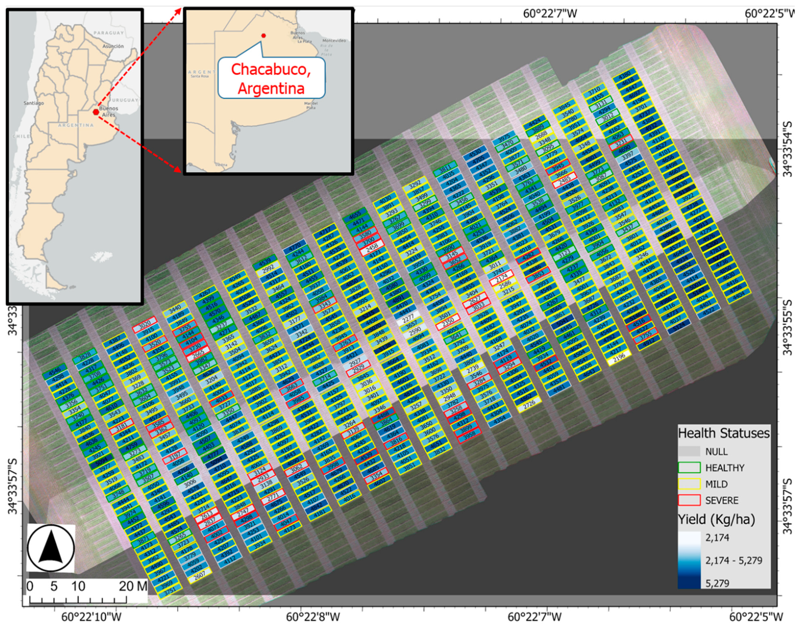
Figure 1. The study site with spring wheats grown in field plots. Inset maps show the location in Chacabuco (−34.64; −60.46), Argentina.
Remotesensing 15 03301 g001
Figure 2. The field of interest (A) and aerial remote sensing platforms included (B) DJI P4 Multispectral (DJI Corporation, Shenzhen, China), (C) the sunlight irradiance sensor, (D) the multispectral sensor mounted to the airframe by an automatic stabilizer.
Remotesensing 15 03301 g002
Figure 3. Close-view pictures of wheat plots labeled in three different categories: healthy (left), mild infection (middle), and severe infection (right).
Remotesensing 15 03301 g003
Figure 4. Random chip images and their spectral profiles of healthy, mild, and severe infection over different times (date format: MM/DD/YYYY).
Remotesensing 15 03301 g004
Figure 5. Disease identification by Deep 3D Convolutional Neural Network (CNN).
Remotesensing 15 03301 g005
Figure 6. Pairwise plots of the five normalized spectral bands (Blue, Green, Red, Red-edge, NIR) by disease status (Healthy, Mild, and Severe infection) over the temporal dimension of (a) 30 August, (b) 24 September, (c) 5 October, (d) 7 October, (e) 26 October, and (f) 17 November.
Remotesensing 15 03301 g006
Figure 7. A dimension-reduction principal component analysis (PCA) transformed the data from a high-dimensional, temporal, and multicollinearity space to a low-dimensional and orthogonal space of 10 principal components. (a) The 10 newly reduced features explained 91% of the original data variance. (b) A 3D scatter plot between three PCA components by disease categories. (c) A heatmap of PCA components influenced by original features (10 most positive influence and another 10 most negative influence).
Remotesensing 15 03301 g007
Figure 8. The overall accuracy (OA) and accuracy of each class as a result of support vector machine (SVM), random forest (RF), multilayer perceptron (MLP), and 3D convolutional neural network (3D-CNN) over temporal datasets (date format: MM/DD/YYYY).
Remotesensing 15 03301 g008
Figure 9. The F1 metrics across four different machine learning algorithms over temporal datasets (date format: MM/DD/YYYY).
Remotesensing 15 03301 g009
Figure 10. Spatial distribution maps of disease statuses. (a) The 700 plots included 592 plots of manually labeled healthy, mild infection, and severe infection and another 108 unknown plots (Null). (b) The 592 plots further spatially and randomly split 80–20 into training (473 plots) and testing (119 plots) during the modelling stage. (c) The trained SVM of temporal-spectral-texture fused data predicting the entire field. (d) The trained RF of temporal-spectral-texture fused data predicting the entire field. (e) The trained MLP of temporal-spectral-texture fused data predicting the entire field. (f) The trained 3D-CNN of temporal UAV imagery predicting the entire field.
Remotesensing 15 03301 g010
Figure 11. The disease-induced impact on yield loss. (a) The harvest yield distribution by wheat disease degrees. (b) Means and standard deviations of wheat yield by disease statuses. (c) A normalized harvest yield by disease statuses on a spatial map.
Remotesensing 15 03301 g011
Figure 12. The actual labeling of severe infection plots (light red) on the test set and its correctly predicted labels (dark red). The test set was randomly assigned 119 plots, among which were 11 severe infection plots. Those infected plots primarily caused permanent yield loss on the crop. UAVs could detect and identify yellow rust at the early stages of the growing season: (a) the SVM correctly predicting 4 out of 11 plots on 30 August, (b) the SVM correctly predicting 3 out of 11 plots on 24 September, (c) the SVM correctly predicting 5 out of 11 plots on 5 October, (d) the SVM correctly predicting 5 out of 11 plots on 7 October, (e) the SVM correctly predicting 3 out of 11 plots on 26 October, and (f) the SVM correctly predicting 6 out of 11 plots on 17 November.
Remotesensing 15 03301 g012
Figure 13. The quantitative estimate of potential yield preservation in Kg/ha and in percentage (%) if the yellow rust can be early detected and properly intervened (date format: MM/DD/YYYY).
Remotesensing 15 03301 g013
Figure 14. Discrepancies in the resolution of UAV aerial images. Within the same collection date, the image resolution collected by one flight mission differed from that collected by another mission. It possibly explained the drop in prediction accuracy from the models used with the 5 October data compared with those used with the 7 October data, especially the image-wise method such as 3D-CNN.
Remotesensing 15 03301 g014
Table 1. Summary of data collection types across crop growing stages in the season.
Dates19 June30 August 24 September 5 October 7 October 26 October 15 November 17 November 16 December
Days of Sowing (DOS)04065777998119121150
Crop Growing StagesPlantingTilleringStem ExtensionStem Extension/
Heading
Stem Extension/
Heading
Heading/
Flowering
FloweringFloweringHarvesting
Data Collection Types UAVUAVUAVUAVUAVHealth Status AnnotationUAVDry Grain Yield
Table 2. Statistical summary of ground truth data on disease statuses and harvesting yield (Kg/ha).
700 Field Plots in TotalTotal Plots
592 Plots Identified Health Status108 Plots Unknown Health Status
HealthyMild InfectionSevere Infection
No. of plots10643056108700
Mean4046.354126.533482.704190.854072.80
STD466.55469.37608.73469.57512.59
CV (%)11.5311.3917.4811.2012.58
Min30122196217422772174
25%3715.2538713054.754038.753801.75
50%41264166.50355042514143
75%4415.754435.753964.7544504420.25
Max50945279453951245279
Table 3. Selected vegetation indices (VIs) extracted from the aerial multispectral images.
No.Index NamesIndex FormulaReference
1Normalized difference vegetation indexndvi = (NIR − R)/(NIR + R)[17]
2Green normalized difference vegetation indexgndvi = (NIR − G)/(NIR + G)[36]
3Ratio vegetation indexrvi_1 = NIR/R[37]
4Green chlorophyll indexgci = (NIR/G) − 1.0[38]
5Red-green ratio vegetation indexrgvi = R/G[39]
6Difference vegetation indexdvi = NIR − R[40]
7Soil-adjusted vegetation indexL = 0.5
savi = ((NIR − R)/(NIR + R + L))×(1.0 + L)
[41]
8Modified soil-adjusted vegetation indexmsavi = 0.5 × ((2.0 × NIR) + 1.0 − ((2.0 × NIR + 1.0)2 − 8.0 × (NIR − R))0.5[42]
9Optimized soil-adjusted vegetation indexosavi = (NIR − R)/(NIR + R + 0.16)[43]
10Renormalized difference vegetation indexrdvi = ((NIR − R)2/(NIR + R))0.5[44]
11Triangular vegetation indextvi = 60.0 × (NIR − G) −100.0 ∗ (R − G)[45]
12Transformed soil-adjusted vegetation indexa, b = 0.96916, 0.084726
tsavi = (a × (NIR − a × R − b))/(a × NIR + R − a × b)
[46]
13Perpendicular vegetation indexa, b = 0.96916, 0.084726
pvi = (NIR − a × R − b)/(1 + (a)2)0.5
[47]
14Soil-adjusted vegetation index 2a, b = 0.96916, 0.084726
savi_2 = NIR/(R − (b/a))
[48]
15Adjusted transformed soil-adjusted vegetation indexa, b, X = 0.96916, 0.084726, 0.08
atsavi = (a × (−a × R − b))/(a × NIR + R − a × b + X × (1 + np.square(a)))
[49]
16Normalized difference water indexndwi = (G − NIR)/(G + NIR)[50]
17normalized total pigment to chlorophyll a ratio indexnpci = (R − B)/(R + B)[51]
18Simple ratio pigment indexsrpi = B/R[51]
19Ratio vegetation index rvi_2 = NIR/G[52]
20Modified chlorophyll absorption ratio index mcari = (RE − R − 0.2 × (RE − G)) × (RE/R)[53]
21Modified chlorophyll absorption ratio index 1 mcari_1 = 1.2 × (2.5 × (NIR − R) − 1.3 × (NIR − G))[54]
22Modified chlorophyll absorption ratio index 2 mcari_2 = 1.5 × (2.5 × (NIR − R) − 1.3 × (NIR − G)) × ((2.0 × NIR + 1)2) − (6.0 × NIR − 5.0 × R) − 0.5[54]
23Modified triangular vegetation index 1 mtvi_1 = 1.2 × (1.2 × (NIR − G) − 2.5 × (R − G))[54]
24Modified triangular vegetation index 2mtvi_2 = 1.5 × (1.2 × (NIR − G) − 2.5 × (R − G)) × ((2 × NIR + 1)2) − (6.0 × NIR−5.0 × R) − 0.5[54]
25Ratio of Modified chlorophyll absorption ratio index and Modified triangular vegetation index 2 r_mcari_mtvi2 = ((RE − R − 0.2 × (RE − G)) × (RE/R))/(1.5 × (1.2 × (NIR−G) − 2.5 × (R − G)) × ((2 × NIR + 1)2) − (6.0 × NIR − 5.0 × R) − 0.5)[55]
26Enhanced vegetation index evi = (NIR − R)/(NIR + 6.0 × R − 7.5 × B + 1.0)[56]
27Datt’s chlorophyll contentdatt = (NIR − RE)/(NIR − R)[57]
28Normalized difference cloud index ndci = (RE − G)/(RE + G)[58]
29Plant senescence reflectance index psri = (R − G)/RE[59]
30Structure insensitive pigment index sipi = (NIR − B)/(NIR + R)[60]
31Spectral polygon vegetation index spvi = 0.4 × 3.7 × (NIR − R) − 1.2 × |G − R|[61]
32Transformed chlorophyll absorption in reflectance index tcari = 3.0 × ((RE − R) − 0.2 × (RE − G) × (RE/R))[62]
33Ratio of TCARI and OSAVIr_tcari_osavi = (3.0 × ((RE − R) − 0.2 × (RE − G) × (RE/R)))/((NIR − R)/(NIR + R + 0.16))[62]
34Red edge relative index reri = (RE − R)/NIR[63]
35Normalized difference red edge index ndre = (NIR − RE)/(NIR + RE)[64]
36MERIS terrestrial chlorophyll index mtci = (NIR − RE)/(RE − R)[65]
37Enhanced vegetation index 2 evi_2 = 2.5 × ((NIR − R)/(NIR + 2.4 × R + 1.0))[66]
38Red edge chlorophyll index reci = (NIR/RE) − 1[38]
39Normalized excess green index nexg = (2 × G − R − B)/(G + R + B)[67]
40Normalized green-red difference indexngrdi = (G − R)/(G + R)[40]
41Enhanced normalized difference vegetation index endvi = (NIR + G − 2.0 × B)/(NIR + G + 2.0 × B)[68]
42Anthocyanin reflectance index 2 ari_2 = NIR × ((1.0/G) − (1.0/RE))[69]
43Carotenoid reflectance index 2 cri_2 = (1.0/G) − (1.0/RE)[70]
Table 4. GLCM texture features [71] extraction.
Texture AttributesFormulasNeighboring DistancesAngularsSpectral BandsTotal
Contrast i , j = 0 l e v e l s 1 P i , j ( i j ) 2 3 values (1, 3, 5)4 angles (0°, 45°, 90°, 135°)5 bands (B, G, R, RE, NIR)60
Dissimilarity i , j = 0 l e v e l s 1 P i , j i j 3 values (1, 3, 5)4 angles (0°, 45°, 90°, 135°)5 bands (B, G, R, RE, NIR)60
Homogeneity i , j = 0 l e v e l s 1 P i , j 1 + ( i j ) 2 3 values (1, 3, 5)4 angles (0°, 45°, 90°, 135°)5 bands (B, G, R, RE, NIR)60
Angular second moment (ASM) i , j = 0 l e v e l s 1 P i , j 2 3 values (1, 3, 5)4 angles (0°, 45°, 90°, 135°)5 bands (B, G, R, RE, NIR)60
Energy A S M 3 values (1, 3, 5)4 angles (0°, 45°, 90°, 135°)5 bands (B, G, R, RE, NIR)60
Correlation i , j = 0 l e v e l s 1 P i , j ( i μ i ) ( j μ j ) ( σ i 2 ) ( σ j 2 ) 3 values (1, 3, 5)4 angles (0°, 45°, 90°, 135°)5 bands (B, G, R, RE, NIR)60
Total Texture Attributes360
Table 5. Summary of one-way ANOVA test on the harvest yield among three health statuses.
Group 1Group 2Mean Differencep ValueLower CIUpper CIReject
HealthyMild80.180.2785−43.05203.403False
HealthySevere−563.65<0.001−751.37−375.93True
MildSevere−643.83<0.001−805.26−482.40True
F-statistic = 43.92, p < 0.001.
Disclaimer/Publisher’s Note: The statements, opinions and data contained in all publications are solely those of the individual author(s) and contributor(s) and not of MDPI and/or the editor(s). MDPI and/or the editor(s) disclaim responsibility for any injury to people or property resulting from any ideas, methods, instructions or products referred to in the content.