Technical Note

Automatic Pear Extraction from High-Resolution Images by a Visual Attention Mechanism Network

1
College of Geography and Remote Sensing Sciences, Xinjiang University, Urumqi 800046, China
2
Xinjiang Key Laboratory of Oasis Ecology, Xinjiang University, Urumqi 830046, China
3
Key Laboratory of Smart City and Environment Modelling of Higher Education Institute, Xinjiang University, Urumqi 830046, China
*
Author to whom correspondence should be addressed.
Remote Sens. 2023, 15(13), 3283; https://doi.org/10.3390/rs15133283
Submission received: 2 June 2023 / Revised: 24 June 2023 / Accepted: 25 June 2023 / Published: 26 June 2023

Abstract

:
At present, forest and fruit resource surveys are mainly based on ground surveys, and the information technology of the characteristic forest and fruit industries is evidently lagging. The automatic extraction of fruit tree information from massive remote sensing data is critical for the healthy development of the forest and fruit industries. However, the complex spatial information and weak spectral information contained in high-resolution images make it difficult to classify fruit trees. In recent years, fully convolutional neural networks (FCNs) have been shown to perform well in the semantic segmentation of remote sensing images because of their end-to-end network structures. In this paper, an end-to-end network model, Multi-Unet, was constructed. As an improved version of the U-Net network structure, this structure adopted multiscale convolution kernels to learn spatial semantic information under different receptive fields. In addition, the “spatial-channel” attention guidance module was introduced to fuse low-level and high-level features to reduce unnecessary semantic features and refine the classification results. The proposed model was tested in a characteristic high-resolution pear tree dataset constructed through field annotation work. The results show that Multi-Unet was the best performer among all models, with classification accuracy, recall, F1, and kappa coefficient of 88.95%, 89.57%, 89.26%, and 88.74%, respectively. This study provides important practical significance for the sustainable development of the characteristic forest fruit industry.

Graphical Abstract

1. Introduction

As a new global trend, precision agriculture is a system supported by information technology in which field information is regularly and quantitatively collected to implement technology and management systems. Precision agriculture mainly involves agriculture and forestry-related global positioning systems, information-collecting systems, remote sensing monitoring systems, geographic information systems, and other subsystems [1,2,3]. Among these methods, the remote sensing technique has become the key technology for acquiring information in precision agriculture systems due to characteristics such as its ability to obtain agricultural and forested planting areas, its ability to conduct repeated monitoring in a short time, its low cost and its capacity to integrate a variety of remote sensing data [4,5]. The combination of remote sensing techniques and modern information technology, such as global positioning systems, can realize the rapid informatization of agricultural land, as well as quantitative studies and analyses, to improve the yield and profit of pear trees. However, complex surface types greatly increase the difficulty of extracting object information in remote sensing applications and using high-resolution remote sensing data to obtain information for use in feature classification has become an important research direction in the fields of remote sensing science and computer vision [6,7,8].
In agriculture research, remote sensing techniques are mainly applied to investigate and plan forest resources, monitor the water use efficiency of farmland, conduct dynamic monitoring and analyses, monitor and develop early-warning systems for disasters, assess disasters, etc. [9,10]. With the continuous progress of remote sensing techniques, multispectral and high-resolution remote sensing data have gradually appeared, providing potential possibilities for information-extraction practices in the forest and fruit industries [11,12]. Hyperspectral images have the advantages of narrow bands and high spectral resolutions and can accurately detect small spectral differences between different ground objects, thus greatly improving the recognition accuracy of objects in forest and fruit research [13,14,15,16,17]. Hyperspectral remote sensing techniques have made great progress in recognition of tree species in the forest and fruit industries, but these techniques cannot meet the statistical accuracy requirements when analyzing spatial areas in forest resource surveys due to their low spatial resolutions. Although unmanned aerial vehicles (UAVs) have rich spectral information and spatial information, due to their small coverage areas and high acquisition costs, it is difficult to use these technologies to meet the needs of large-scale forest and fruit industry surveys [18,19]. Comparatively speaking, high-resolution remote sensing images not only have obvious spectral characteristics but can also output prominent information on ground object shapes, structures, and textures. As in-depth research on remote sensing image processing and classification methods has progressed, it has been difficult to meet the needs of high-precision remote sensing classifications by relying only on the spectral information contained in images. Therefore, the rich spatial semantic information contained in high-resolution remote sensing images plays an increasingly important role in classification and recognition techniques [20,21,22,23,24]. However, it is difficult to extract semantic information from high-resolution remote sensing images because differences in the shapes and structures of different ground objects are multiscale in remote sensing images and because of the high correlations and redundancies that occur between image texture features. Therefore, effective feature extraction methods directly affect the classification and recognition accuracies and are the key to investigating and extracting information of forest resources, such as in area extractions of tree species in remote sensing, growth monitoring, yield estimation, and pest control applications [25,26,27,28,29,30,31,32].
With the rapid development of artificial intelligence and big data, deep learning has become a widely used method in the fields of computer vision, autonomous driving, speech recognition and feature extraction by means of multilayer nonlinear information processing, and an end-to-end application model has gradually been formed based on a large number of samples [33,34,35]. In addition, deep learning also plays an important role in processing remote sensing images [28,36,37,38,39,40]. In particular, after Long et al. proposed the fully convolutional neural network (CNN) model [41], the CNN with the encoder-decoder framework was used to extract specific image features by simulating the human visual system to perform hierarchical abstract processing on original images. This method has been widely used in remote sensing image classifications, target object detections, scene recognitions, and other tasks and has gradually become a means by which the semantic segmentation of remote sensing images can be performed [42,43]. Compared to traditional object-oriented and pixel-oriented classification methods [44,45,46], CNN-based networks typically achieve higher classification accuracy. For example, SegNet, FCN8s, and U-Net utilize automatic feature learning to avoid complex feature design, improving the automation and intelligence of remote sensing image segmentation [47]. Consequently, CNNs are gaining increasing attention for feature information extraction in remote sensing applications [7,48,49].
While CNNs have shown success in classifying high-resolution remote sensing images, several problems remain. Firstly, CNNs depend heavily on the number of input training samples, which are limited for remote sensing images, making generalization difficult [47,50]. Secondly, most models have been trained on natural image datasets and are not suitable for remote sensing images [51]. Finally, contextual information needs to be combined for interpretation, but existing models have limited receptive neuron fields and insufficient multiscale feature-learning abilities [52,53,54].
In this study, by improving the U-Net network, we proposed a multiscale CNN model to extract the distribution area of pear trees. Specifically, convolutional kernels of different sizes were used to expand the receptive field to obtain more context features in the input images, and lower-level and higher-level features were fused by residual means to reduce the transmission of redundant features in the network. On the other hand, because the attention mechanism could effectively focus on useful information and ignore redundant information in the network-training process by simulating the process of human visual perception, the construction of a “spatial-channel” attention guidance module could eliminate the semantic differences among different feature levels and assist in the selection of important features to optimize the Multi-Unet classification results.
The rest of this paper is arranged as follows: In the second part, the research area and data acquisition method are described. In the third section, we introduce detailed information on the Multi-Unet method. In the fourth part, we test and analyze the availability of this method on the Gaofen (GF)-6 dataset. Finally, conclusions are drawn in the fifth section.

2. Materials and Study Area

2.1. Study Area

Yuli County is located in the Bayingoleng Mongol Autonomous Prefecture of the Xinjiang Uygur Autonomous Region and has geographical coordinates of 84°02′E~89°58′E, 40°10′N~41°39′N and a total area of 59,700 square kilometers. This region belongs to a temperate continental desert climate zone. Great differences between heat and cold conditions occur in this area, along with strong evaporation and sufficient light. The average sunshine duration is 2975 h a year, and due to the unique climate conditions, it is rich in crops, such as fragrant pear, cotton, and licorice. Pear trees are deciduous fruit trees, and due to their need to drop their leaves and become dormant in winter, for better observation and analysis, the remote sensing image data recorded by the GF-6 satellite on 15 May 2019 was selected in this study. After the images were corrected, fused, and preprocessed, their spatial resolution was 2 m, and they included four bands, the near-infrared, red, blue, and green bands, as shown in Figure 1.

2.2. Labeled Data Acquisition and Production

The production of representative training sample data is a crucial part of semantic segmentation for deep learning applications. High-resolution remote sensing images contain complex spatial textures and other information. When constructing a sample set, it is important to include all feature types in the study area and to distribute representatives of each feature type as evenly as possible. This is necessary because the spatial, geometric, and spectral features of different objects vary significantly in different regions, and the “same subject with different spectra” and “same spectra with different subjects” phenomena in remote sensing images present great challenges to the accuracy and performance of feature recognition methods, which, in turn, highlights the importance of a well-constructed sample set.
The process by which a dataset sample is generated mainly includes field sample site tagging and the indoor production of label sets. To ensure the scientific validity of the sample site selection process and the accuracy of pear tree identification, a field survey was conducted in Yuli County to determine the distribution range of pear trees and the actual conditions surrounding the captured images. The experimental area was chosen in the region with the highest concentration of pear trees in Yuli County. GPS points were used to mark all the experimental tags in the field. Based on the marked point data and a vegetation-type distribution map of Yuli County, the region was subdivided using indoor visual interpretation. Edge information was collected as accurately as possible, and the experimental area images were divided into pear orchards and other areas to complete the tagging process. After this process, the original images had the same sizes and dimensions as the tagged images.

3. Methods

The reasonable and correct use of contextual information in remote sensing images is the key to improving semantic segmentation. Currently, many scholars use the dilated convolution method to expand the receptive field. However, this process leads to the loss of local information, resulting in poor image segmentation. When there are too many layers in a model, a large amount of redundant information can easily be transferred from the lower layers to the deeper layers, thus affecting the credibility of the model.

3.1. Network Structure

The Multi-Unet encoder is mainly based on the improved U-Net network model and can be divided into different feature blocks according to the output feature map. The network structure is shown in Figure 2. The spatial sizes of the images range from 512 × 512 pixels to 32 × 32 pixels, and the features closer to the input layer contain more bottom-level information. Conversely, the features closer to the output layer contain more top-level information. Multi-Unet makes the following improvements to the original U-Net network: First, the original two 3 × 3 convolution kernel operations are uniformly replaced by a convolution block that consists of 1 × 1, 3 × 3, 5 × 5, and 7 × 7 convolutional layers and cross-channel integration is performed by 1 × 1 to ensure the effectiveness of feature information extraction while simplifying the computational complexity of the model. Meanwhile, because feature extraction has a certain geospatial correlation, the extraction of pear tree feature information can be further enhanced by expanding the receptive field. Then, 3 × 3, 5 × 5, and 7 × 7 convolution kernels are used for further in-depth feature extraction [55]. The purpose of this replacement is to learn the semantic information of images at different scales at each feature-level stage.
In addition, a “spatial-channel” attention guidance module is added to the decoder part of the U-net network. This link between channel and space is established to strengthen important feature information and weaken nonimportant feature information to present semantic information that is useful for feature extraction. The encoder part continuously compresses the feature information of the image by convolution and pooling, while the decoder recovers the feature map resolution by transposed convolution and upsampling operations using the “spatial-channel” attention guidance module. A skip connection exists between the encoder and the decoder. This connection fuses the shallow simple features with the deep abstract features in the network to help the decoder better restore the target details. The “spatial-channel” attention bootstrap of the entire network uses the sigmoid activation function, the output layer uses the softmax activation function, and all the remaining convolutional layers use the ReLu activation function.

3.2. “Spatial-Channel” Attention Guidance Module

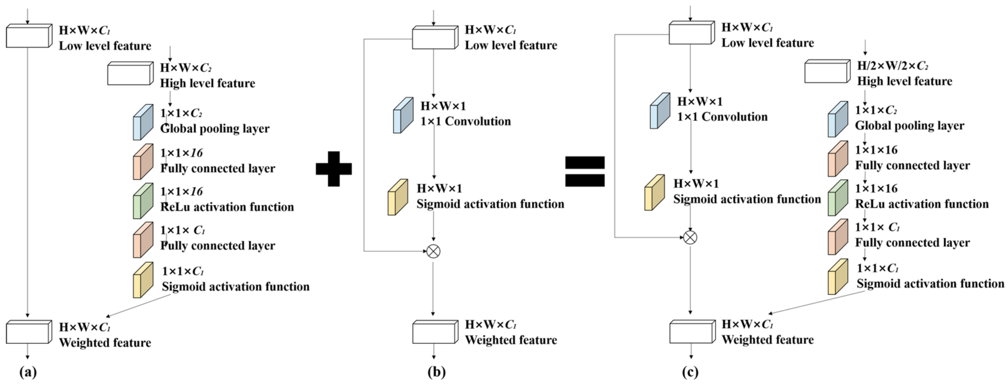
The channel attention guidance module is a multilevel feature-fusion unit that is based on the squeeze-and-excitation (SE) module and is mainly used to eliminate the semantic differences between different feature levels and to extract important features [56,57]. In this module, both high-level and low-level features participate in the feature-weighting process.
Specifically, the channel attention guidance module first converts high-level features U c into a one-dimensional weighted feature vector by “aggregation” using the following expression:
q c = F s q U c = 1 w / 2 × h / 2 i = 1 w / 2 j = 1 h / 2 u c i , j
where I is the low-level feature mapping, I R h × w × C 1 , U is the high-level feature mapping, I R h / 2 × w / 2 × C 2 , q c denotes the average of all image elements contained in the cth channel of the feature map q and is used to indicate the value distribution of the feature map contained in this channel, i.e., its contextual information.
After the aggregation process, the next step is “expansion”, which is performed using the following calculation:
s = F e x q , W = σ g q , W = σ W 2 δ W 1 q
where δ and σ are the ReLu and sigmoid layers, respectively. By multiplying the q R 1 × 1 × C 2 expression obtained in Equations (2)–(4) with W 1 R 16 × C 2 , a fully connected layer operation, W 1 q R 1 × 1 × 16 , can be obtained using the activation function δ . The data dimension remains unchanged, and by again multiplying this expression with W 2 R C 1 × 16 in a fully connected layer process, we get W 1 q R 1 × 1 × 16 . After applying the activation function σ , the data dimensions remain unchanged. At this moment, the input data are first dimensionally reduced and then dimensionally expanded so that the input and output dimensions remain the same.
The obtained weight s in the above equation is the core of the channel attention mechanism. By learning the feature information in the fully connected layer and the nonlinear activation function layer to obtain the weights of the feature map and by multiplying the weight s with the input feature map U, it is possible to assign different weights to each channel in the feature map with the following equation:
x c = F s c a l e U c , s c = U c × s c
where x = x 1 , x 2 , , x c 1 denotes the weighted fused features, as shown in Figure 3a, and the weighted fused features are passed to the subsequent network after the convolution operation.
In the spatialwise attention guidance module, as shown in Figure 3b, the multichannel feature map I is compressed into a single-channel feature after the convolution of channel number 11, and a spatial squeezing operation is realized as follows:
q = C × I
where C is the convolution layer, C R 1 × 1 × c × 1 , I , I R H × W × c , and q is the feature map with channel number 1.
The weights are normalized to range from [0, 1] using the sigmoid function, and each channel feature is multiplied with the corresponding weight to obtain a new feature channel:
x c = F s s e q c , I c = σ q c × I c
where x = x 1 , x 2 , , x c denotes the weighted fused features and σ is the sigmoid function. In this way, each obtained   x c value is associated with the spatial information contained in the initial feature map, and this kind of spatialwise attention guidance module gives more weight to the relevant spatial information and ignores the irrelevant spatial information.
In this paper, we took GF-6 for pear tree extraction. Due to the difference in the response of vegetation to different bands of spectra, it has a strong sensitivity. In this way, we combine the channel attention guidance module with the spatialwise attention guidance module to obtain the “spatial-channel” attention guidance module, as shown in Figure 3c. This module is then used to weight the spatial-dimension and channel-dimension features to eliminate the semantic discrepancy problem in the images and to avoid the generation of redundant features. Thus, the pear tree feature extraction in this way for high-resolution images can speed up the model convergence speed and improve the classification accuracy of the model.

3.3. Evaluation Index

To measure the pear tree identification effectiveness, we used four evaluation metrics, precision, recall, the F1 score, and the kappa coefficient, to evaluate the Yuli County pear tree dataset. Precision is a measure of the proportion of the number of samples that were correctly predicted to be positively classified to the number of all samples that were predicted to be positively classified. When the predicted values of all samples exactly match the true values of all samples, the precision is 1.0, and otherwise, the precision is 0.0. Recall is the proportion of the number of samples that is correctly predicted to be positively classified to the number of all positive samples. The F1 score is the combined precision and recall score and is calculated by summing precision and recall. The kappa coefficient is often used for consistency testing and for determining the classification accuracy. The kappa coefficient is usually calculated based on a confusion matrix. The calculation formulas used to obtain these metrics are as follows.
r e c a l l k = T P k T P k + F N k
p r e c i s i o n k = T P k T P k + F P k
F 1 = 1 + β 2 r e c a l l p r e c i s i o n β 2 r e c a l l + p r e c i s i o n , β = 1
K a p p a = p o p e 1 p e
where T P k is the true positives (TPs) of class k, indicating the number of pixels whose predicted pixel values agree with the true pixel values. F P k is the false positives (FPs) of class k, indicating the number of non-k pixels incorrectly identified as class k pixels. F N k is the false negatives (FNs) of class k, indicating the failure to identify class k pixels. F N k and β are usually assigned a value of 1, representing the accuracy weight. p o denotes the number of correctly classified samples (diagonal values) in the confusion matrix divided by the number of samples, and p e   denotes the total number of samples divided by two after multiplying the true values of each class and the predicted values of each class in the confusion matrix.

4. Experiments and Results

This experiment was carried out on the Kaggle online website (www.kaggle.com), the graphics processing unit (GPU) was the NVIDIA Nvidia Tesla P100-PCIE-16GB, the programming language was Python, and the deep learning framework was compiled with TensorFlow 2.0. The model was uniformly trained using the Adam optimizer. The number of iterations of each model was 50. The verification accuracy was calculated once per iteration. The model weight with the best accuracy was retained in each iteration, and binary cross entropy was applied as the loss function. The training and test sets were input to the network structure in the form of image data. To analyze and test the impacts of different input image sizes on the classification results, two different image sizes, 256 × 256 pixels, and 512 × 512 pixels, were selected as inputs.
In our experiment, the current mainstream network models were selected for comparison, SegNet [58], FCN8s [41,59,60], U-Net [61], Res-U-Net [37], PSPNet [62], RefineNet, and DeepLabv3+ [63,64,65]. These models have been widely used in research on the semantic segmentation of remote sensing images. All models are open-source and can be modified according to the number of bands in the input images.

4.1. Single Module Functional Comparison

In this section, we tested the use of A: Spatialwise attention guidance module, B: Channel attention guidance module, and C: “Spatial-channel” attention Results of guidance module in Unet. The experimental results are shown in Table 1. Because C combines multi-scale feature information at the same time and adopts a channel attention mechanism to suppress redundant feature information, the confidence of key features is greatly improved, so it achieves the best performance. In addition, all indexes of B are higher than those of A, which also indicates that increasing the channel attention mechanism can lead to better performance in the network.

4.2. Pear Tree Extraction from GF-6 Data

4.2.1. Data Enhancement

Data augmentation is an essential step in deep learning tasks. In the actual production process, it takes considerable time to manually construct samples. Generating new data through data enhancement without changing the sample labels can effectively expand the amount of data so that the model can enhance its generalization ability and classification accuracy during training. Current deep-learning methods offer a large number of expansion interfaces for data. However, due to the particularity of remote sensing images, it is necessary to select a data enhancement method for use in the classification task according to the actual situation to avoid generating too many redundant samples, which would reduce the model classification accuracy and the model-training efficiency. Instead, we choose an effective data enhancement method, superimpose another method on the basis of one data enhancement method, and attempt to differentiate the transformed image from the original image as much as possible. At the same time, a certain ratio is set for data enhancement according to the number of each sample, and finally, the sample ratio of each category reaches a balanced state. The data enhancement methods used in this process include geometric enhancement and pixel enhancement. Geometric enhancement includes the rotation, enlargement, reduction, and distortion of images. Pixel enhancement includes the blurring, sharpening, noise addition, and saturation manipulation of images.

4.2.2. Result of the GF-6 Data

Figure 4 shows the classification results of different FCN models on the Yuli County dataset. Compared with other models, whether the input size is 256 × 256 pixels or 512 × 512 pixels, the Multi-Unet network and DeepLabv3+ achieve the best results on the dataset. The classification results of the SegNet and FCN8s network models both showed an obvious “salt and pepper” phenomenon. The SegNet and FCN8s networks had large areas of false negative pixels, and the number of pixels in which pear trees failed to be identified was the largest. The network model had a 512 × 512 pixel size class area and even more false negatives, indicating that improving the semantic image segmentation performance by using shallower network layers and simple upsampling convolution operations is difficult. U-Net also uses the upsampling convolution operation, but it transfers feature information through a “jumping” connection between the encoder and the decoder, and its classification effect is significantly better than those of SegNet and FCN8s. However, obvious misclassifications and omissions still occur with this method, and a large number of false positive pixels appear. For example, some water bodies and Populus euphratica forests were mistakenly classified as pear trees, some pear trees were not detected, and the pear tree detection was incomplete. When the input size of the Res-U-Net was 256 × 256 pixels, the accuracy was significantly higher than 512 × 512 pixels, especially between different fruit trees. DeepLabv3+ uses the “hole” convolution method to obtain the contextual information of a relatively large receptive field, resulting in a better recognition effect on pear trees. However, some false positive and false negative pixels still occur.
Figure 5 shows the enlarged classification results of different FCN models in the local area of the pear dataset in Yuli County. The Multi-Unet and DeepLabv3+ models can accurately identify the distribution range of pear trees, and the boundary contour information of pear trees is clear under these methods. When the input size was 256 × 256, the accuracy of the Multi-Unet network was highest. DeepLabv3+ output some false positive and false negative pixels in the pear tree identification process. Compared with the previous two models, the misclassifications and omissions performed by other models were more obvious. The geometric characteristics of pear trees were similar to those of fruit forests, such as jujube trees, causing the image resolution to affect the pear tree classification accuracy. This phenomenon shows that the combined multilevel and multiscale feature-extraction methods can improve the accuracy of the model.
Table 2 lists the classification accuracy of the FCN model on the GF-6 Yuli County pear tree test dataset. The article uses four indicators to evaluate the classification accuracy of the model, including the classification accuracy, recall, F1 score, and kappa coefficient. When the input image size of the Multi-Unet network was 256 × 256, the classification accuracy, recall rate, F1, and kappa coefficients were 88.95%, 89.57%, 89.26% and 88.74%, respectively, representing the highest accuracy among all models. When the input image size was 256 × 256, the F1 and kappa coefficients of the DeepLabv3+ model were 86.07% and 85.42%, respectively, second only to those of Multi-Unet at the same input size. When the input image size was 512 × 512, the kappa coefficient of Multi-Unet was slightly higher than that of DeepLabv3+, and the F1 score of Multi-Unet was slightly lower than that of DeepLabv3+. The classification accuracies of the Res-U-Net and U-Net models were relatively close. When the input image size was 512 × 512, FCN8s had an accuracy of 90.53%, the highest accuracy among all models, but the kappa coefficient and F1 score were only 68.39% and 69.51%, respectively, and the recall was only 56.41%. This poor extraction performance indicates that the image classification results need to be improved. Among many models, when the size of the images input to model was 256 × 256, the accuracy of the model was generally better than when the input image size was 512 × 512.

4.2.3. The Impacts of Different Band Combinations on the Model Classification Accuracy

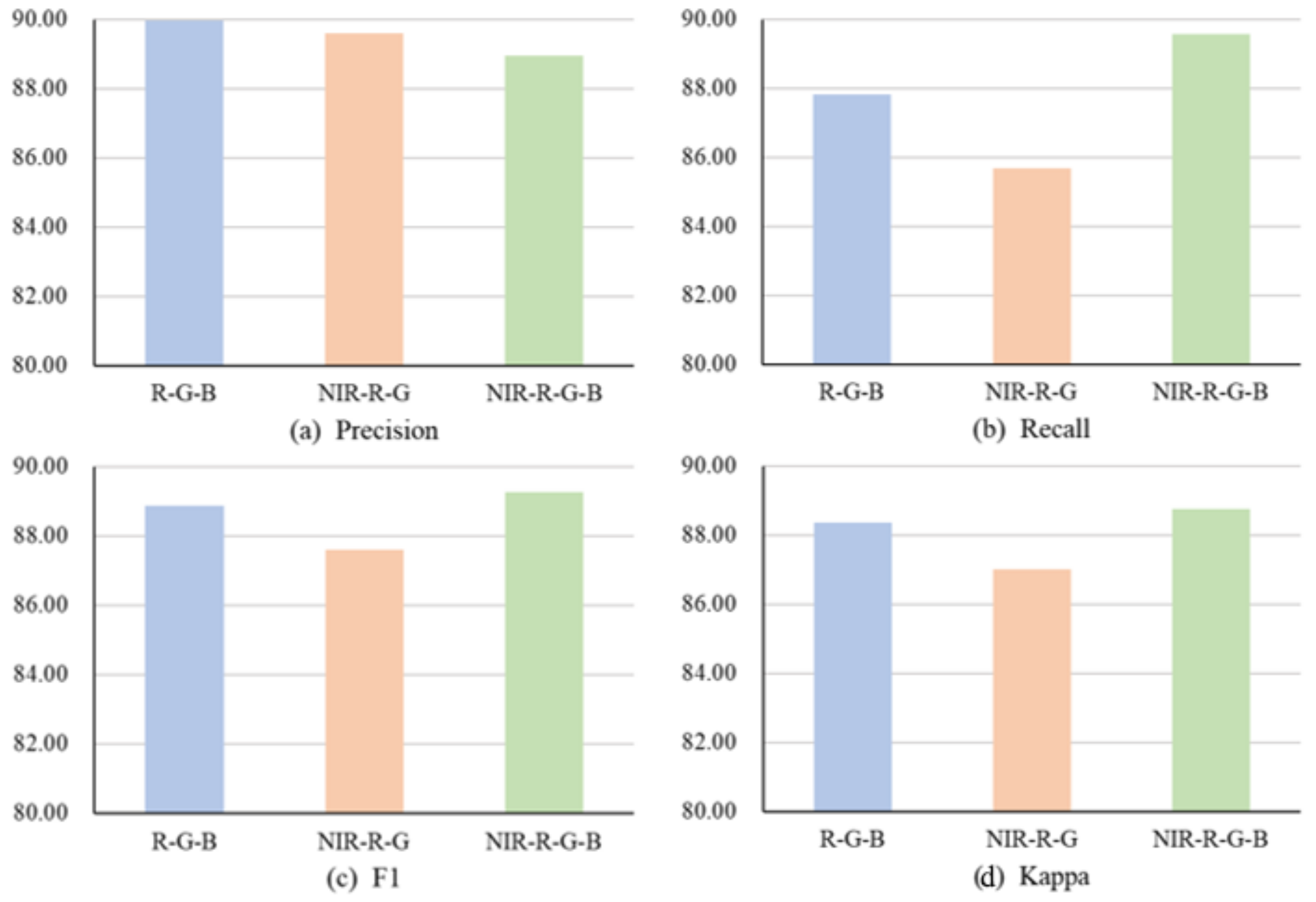
Figure 6 shows the accuracy evaluation results of Multi-Unet under different input band combinations. In general, when using a combination of the four-band NIR-R-G-B model, the best performance was achieved. Compared with R-G-B, the three-band recall was 1.76% higher, and the F1 and kappa coefficients were slightly higher than those of R-G-B. These results indicate that increasing the number of bands significantly affects the pear tree classification results.

4.3. Tree Extraction from Potsdam Data

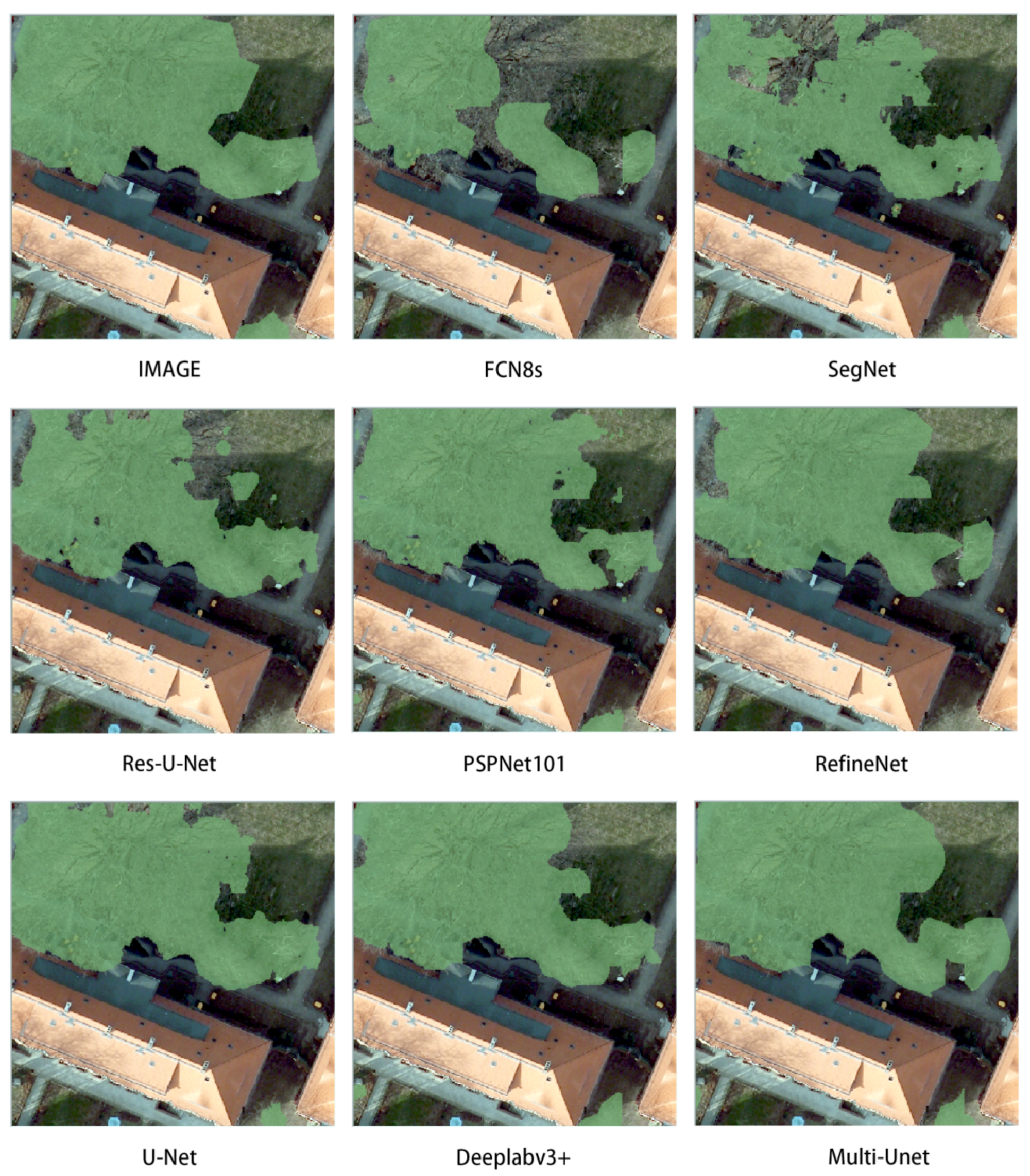
In order to further verify the universality of the model, we also conducted a comparative analysis between Multi-Unet and other methods in Table 3, in which we only analyzed the effect of tree in Potsdam data [66]. In general, the richer the spatial-spectral information in the dataset, the higher the accuracy of the model. However, Figure 7 shows shallower models, such as FCN8s, tend to produce fragmented information, and the predicted targets are noisy and irrelevant. Multi-U-Net uses residuals to obtain image context information, which alleviates this phenomenon, making the predicted object boundary smoother and more reliable. In addition [67], compared to other algorithms, FCN8 requires fewer computing resources, mainly due to the model using a shallower network structure. The required parameters of DeepLabv3+ were relatively large because it uses the Xception block in the encoding stage, thus greatly increasing the network complexity. Although Multi-Unet also uses different convolution kernel sizes in the encoding and decoding processes, thanks to the addition of a 1 × 1 convolution kernel, the number of model parameters was reduced, and the model size required only 28.34 MB. PSPNet uses a pyramid pool module to obtain multiscale spatial information, but this improvement also increases the complexity of the network. Overall, Multi-Unet is more efficient than most other models.

4.4. Model Analysis

The effective integration of features and feature-selection methods is very important to improve the learning efficiency and classification accuracy of FCN models. Compared to other models, the Multi-Unet network has the following advantages. First, Multi-Unet is an improved version based on the U-net network in which the spatial dimension of the pooling layer is reduced in the encoder stage. The decoder gradually repairs the details and spatial dimensions of the object. However, as the number of layers gradually deepens, this structure loses a large amount of its spatial feature information, resulting in abnormally rough edges in the image classification results. When combined with the residual network structure, Multi-Unet breaks the convention that the output of the n-1 layer in a traditional neural network can take only n layers as the input. Thus, in Multi-Unet, the output of a certain layer can directly cross several layers as the input of a subsequent layer. As the number of network layers increases, the number of feature maps progressively increases layer-by-layer, thus ensuring the expressive ability of the output features and allowing the accuracy to be maintained even as the depth increases. At the same time, for most current network models, the filter size is relatively fixed when extracting feature information. However, the sizes and shapes of similar objects in remote sensing images are often quite different, and convolution kernels of different sizes are used to mine the spatial contextual information of the images. Second, after fusing the low-level features with the high-level features, the attention mechanism is used to weigh these features to reduce the semantic differences among different levels. Such weighted features not only retain rich, detailed, bottom-level spatial information but also effectively eliminate redundant information, thus providing a good foundation for subsequent feature selection and classification accuracy improvements. Therefore, Multi-Unet can handle the semantic segmentation problems associated with high-resolution remote sensing images.

5. Conclusions

As an important machine-learning branch, deep learning is widely used in semantic segmentation tasks involving high-resolution remote sensing images due to advantages such as automatic feature extraction, high efficiency, and fitting of complex nonlinear functions. Based on summarizing the status quo of high-resolution remote sensing image classification methods, this paper constructs a high-resolution pear tree dataset and proposes a new end-to-end network structure called Multi-Unet to extract pear trees from these data. The “spatial-channel” attention guidance module was used to fuse the low-level features and high-level features in the encoder and decoder to allow the fused features to have higher category credibility and to reduce the presence of redundant information. Second, by using different convolution kernels of different sizes to mine local and global features, complex spatial contextual information can be effectively extracted. The results show that Multi-Unet had a strong fruit tree extraction performance and could effectively monitor the distribution area of pear trees in Yuli County. This study provided a certain reference basis for the dynamic monitoring of the crop area changes in the fruit industry.
In this paper, we have only focused on the feature extraction part, and there has been no in-depth study on the jump connection of the upsampling part of the image [68]. Whether we can fully integrate the previous information with upsampling and increase the restoration degree in the image restoration process through various forms of upsampling connections is the focus of my future research. Although we have compressed the model, we have not reached the ultimate level, and there is still room for further compression. In the follow-up work, we can refer to other related work to further compress the overall number of parameters of the model.

Author Contributions

Conceptualization, J.W. and J.D.; methodology, J.W.; software, S.R.; validation, J.W., S.Q. and X.L.; formal analysis, S.R.; investigation, S.R.; resources, J.D.; data curation, B.L.; writing—original draft preparation, J.W.; writing—review and editing, J.D.; visualization, S.Q.; supervision, J.D.; project administration, J.W.; funding acquisition, J.W. All authors have read and agreed to the published version of the manuscript.

Funding

This research was funded by the National Natural Science Foundation of China Joint Fund Key Project (No. U2003202), Key Project of Natural Science Foundation of Xinjiang Uygur Autonomous Region (No. 2020D04038), and the Key Research Projects for Teachers of Universities in Autonomous Regions (No. XJEDU2021Y009).

Data Availability Statement

Data sharing is not applicable to this article.

Acknowledgments

We are sincerely grateful to the reviewers and editors for their constructive comments on the improvement of the manuscript.

Conflicts of Interest

The authors declare no conflict of interest.

References

  1. Sishodia, R.P.; Ray, R.L.; Singh, S.K. Applications of Remote Sensing in Precision Agriculture: A Review. Remote Sens. 2020, 12, 3136. [Google Scholar] [CrossRef]
  2. Tsouros, D.C.; Bibi, S.; Sarigiannidis, P.G. A Review on UAV-Based Applications for Precision Agriculture. Information 2019, 10, 349. [Google Scholar] [CrossRef] [Green Version]
  3. Liaghat, S.; Balasundram, S.K. A review: The role of remote sensing in precision agriculture. Am. J. Agric. Biol. Sci. 2010, 5, 50–55. [Google Scholar] [CrossRef] [Green Version]
  4. Khanal, S.; Fulton, J.; Shearer, S. An overview of current and potential applications of thermal remote sensing in precision agriculture. Comput. Electron. Agric. 2017, 139, 22–32. [Google Scholar] [CrossRef]
  5. Seelan, S.K.; Laguette, S.; Casady, G.M.; Seielstad, G.A. Remote sensing applications for precision agriculture: A learning community approach. Remote Sens. Environ. 2003, 88, 157–169. [Google Scholar] [CrossRef]
  6. Segarra, J.; Buchaillot, M.L.; Araus, J.L.; Kefauver, S.C. Remote Sensing for Precision Agriculture: Sentinel-2 Improved Features and Applications. Agronomy 2020, 10, 641. [Google Scholar] [CrossRef]
  7. Huang, J.; Zhang, X.; Xin, Q.; Sun, Y.; Zhang, P. Automatic building extraction from high-resolution aerial images and LiDAR data using gated residual refinement network. ISPRS J. Photogramm. Remote Sens. 2019, 151, 91–105. [Google Scholar] [CrossRef]
  8. Bagheri, N. Development of a high-resolution aerial remote-sensing system for precision agriculture. Int. J. Remote Sens. 2017, 38, 2053–2065. [Google Scholar] [CrossRef]
  9. Qin, S.; Ding, J.; Ge, X.; Wang, J.; Wang, R.; Zou, J.; Tan, J.; Han, L. Spatio-Temporal Changes in Water Use Efficiency and Its Driving Factors in Central Asia (2001–2021). Remote Sens. 2023, 15, 767. [Google Scholar] [CrossRef]
  10. Zhou, Q.-B.; Yu, Q.-Y.; Liu, J.; Wu, W.-B.; Tang, H.-J. Perspective of Chinese GF-1 high-resolution satellite data in agricultural remote sensing monitoring. J. Integr. Agric. 2017, 16, 242–251. [Google Scholar] [CrossRef]
  11. Holmgren, P.; Thuresson, T. Satellite remote sensing for forestry planning—A review. Scand. J. For. Res. 1998, 13, 90–110. [Google Scholar] [CrossRef]
  12. Wen, D.; Huang, X.; Liu, H.; Liao, W.; Zhang, L. Semantic Classification of Urban Trees Using Very High Resolution Satellite Imagery. IEEE J. Sel. Top. Appl. Earth Obs. Remote Sens. 2017, 10, 1413–1424. [Google Scholar] [CrossRef]
  13. Ge, X.; Ding, J.; Teng, D.; Wang, J.; Huo, T.; Jin, X.; Wang, J.; He, B.; Han, L. Updated soil salinity with fine spatial resolution and high accuracy: The synergy of Sentinel-2 MSI, environmental covariates and hybrid machine learning approaches. CATENA 2022, 212, 106054. [Google Scholar] [CrossRef]
  14. Ge, X.; Ding, J.; Jin, X.; Wang, J.; Chen, X.; Li, X.; Liu, J.; Xie, B. Estimating Agricultural Soil Moisture Content through UAV-Based Hyperspectral Images in the Arid Region. Remote Sens. 2021, 13, 1562. [Google Scholar] [CrossRef]
  15. Sothe, C.; De Almeida, C.M.; Schimalski, M.B.; La Rosa, L.E.C.; Castro, J.D.B.; Feitosa, R.Q.; Dalponte, M.; Lima, C.L.; Liesenberg, V.; Miyoshi, G.T.; et al. Comparative performance of convolutional neural network, weighted and conventional support vector machine and random forest for classifying tree species using hyperspectral and photogrammetric data. GIScience Remote Sens. 2020, 57, 369–394. [Google Scholar] [CrossRef]
  16. Fricker, G.A.; Ventura, J.D.; Wolf, J.A.; North, M.P.; Davis, F.W.; Franklin, J. A Convolutional Neural Network Classifier Identifies Tree Species in Mixed-Conifer Forest from Hyperspectral Imagery. Remote Sens. 2019, 11, 1562. [Google Scholar] [CrossRef] [Green Version]
  17. Paul, N.C.; Sahoo, P.M.; Ahmad, T.; Sahoo, R.; Krishna, G.; Lal, S. Acreage estimation of mango orchards using hyperspectral satellite data. Indian J. Hortic. 2018, 75, 27–33. [Google Scholar] [CrossRef]
  18. Jiang, Y.; Zhang, L.; Yan, M.; Qi, J.; Fu, T.; Fan, S.; Chen, B. High-Resolution Mangrove Forests Classification with Machine Learning Using Worldview and UAV Hyperspectral Data. Remote Sens. 2021, 13, 1529. [Google Scholar] [CrossRef]
  19. Yu, N.; Li, L.; Schmitz, N.; Tian, L.F.; Greenberg, J.A.; Diers, B.W. Development of methods to improve soybean yield estimation and predict plant maturity with an unmanned aerial vehicle based platform. Remote Sens. Environ. 2016, 187, 91–101. [Google Scholar] [CrossRef]
  20. Dong, Y.; Liu, Q.; Du, B.; Zhang, L. Weighted Feature Fusion of Convolutional Neural Network and Graph Attention Network for Hyperspectral Image Classification. IEEE Trans. Image Process. 2022, 31, 1559–1572. [Google Scholar] [CrossRef]
  21. Yan, J.; Wang, L.; Song, W.; Chen, Y.; Chen, X.; Deng, Z. A time-series classification approach based on change detection for rapid land cover mapping. ISPRS J. Photogramm. Remote Sens. 2019, 158, 249–262. [Google Scholar] [CrossRef]
  22. Son, N.-T.; Chen, C.-F.; Chen, C.-R.; Minh, V.-Q. Assessment of Sentinel-1A data for rice crop classification using random forests and support vector machines. Geocarto Int. 2018, 33, 587–601. [Google Scholar] [CrossRef]
  23. Battude, M.; Al Bitar, A.; Morin, D.; Cros, J.; Huc, M.; Marais Sicre, C.; Le Dantec, V.; Demarez, V. Estimating maize biomass and yield over large areas using high spatial and temporal resolution Sentinel-2 like remote sensing data. Remote Sens. Environ. 2016, 184, 668–681. [Google Scholar] [CrossRef]
  24. Sibanda, M.; Mutanga, O.; Rouget, M. Examining the potential of Sentinel-2 MSI spectral resolution in quantifying above ground biomass across different fertilizer treatments. ISPRS J. Photogramm. Remote Sens. 2015, 110, 55–65. [Google Scholar] [CrossRef]
  25. Wang, R.; Ding, J.; Ge, X.; Wang, J.; Qin, S.; Tan, J.; Han, L.; Zhang, Z. Impacts of climate change on the wetlands in the arid region of Northwestern China over the past 2 decades. Ecol. Indic. 2023, 149, 110168. [Google Scholar] [CrossRef]
  26. Hassan, S.M.; Maji, A.K. Plant Disease Identification Using a Novel Convolutional Neural Network. IEEE Access 2022, 10, 5390–5401. [Google Scholar] [CrossRef]
  27. Arce, L.S.D.; Osco, L.P.; Arruda, M.d.S.d.; Furuya, D.E.G.; Ramos, A.P.M.; Aoki, C.; Pott, A.; Fatholahi, S.; Li, J.; Araújo, F.F.d.; et al. Mauritia flexuosa palm trees airborne mapping with deep convolutional neural network. Sci. Rep. 2021, 11, 19619. [Google Scholar] [CrossRef] [PubMed]
  28. Kattenborn, T.; Leitloff, J.; Schiefer, F.; Hinz, S. Review on Convolutional Neural Networks (CNN) in vegetation remote sensing. ISPRS J. Photogramm. Remote Sens. 2021, 173, 24–49. [Google Scholar] [CrossRef]
  29. Li, H.; Zhang, C.; Zhang, S.; Atkinson, P.M. Crop classification from full-year fully-polarimetric L-band UAVSAR time-series using the Random Forest algorithm. Int. J. Appl. Earth Obs. Geoinf. 2020, 87, 102032. [Google Scholar] [CrossRef]
  30. Sidike, P.; Sagan, V.; Maimaitijiang, M.; Maimaitiyiming, M.; Shakoor, N.; Burken, J.; Mockler, T.; Fritschi, F.B. dPEN: Deep Progressively Expanded Network for mapping heterogeneous agricultural landscape using WorldView-3 satellite imagery. Remote Sens. Environ. 2019, 221, 756–772. [Google Scholar] [CrossRef]
  31. Lakmal, D.; Kugathasan, K.; Nanayakkara, V.; Jayasena, S.; Perera, A.S.; Fernando, L. Brown Planthopper Damage Detection using Remote Sensing and Machine Learning. In Proceedings of the 2019 18th IEEE International Conference On Machine Learning And Applications (ICMLA), Boca Raton, FL, USA, 16–19 December 2019; pp. 97–104. [Google Scholar]
  32. Hariharan, S.; Mandal, D.; Tirodkar, S.; Kumar, V.; Bhattacharya, A.; Lopez-Sanchez, J.M. A Novel Phenology Based Feature Subset Selection Technique Using Random Forest for Multitemporal PolSAR Crop Classification. IEEE J. Sel. Top. Appl. Earth Obs. Remote Sens. 2018, 11, 4244–4258. [Google Scholar] [CrossRef] [Green Version]
  33. Zhang, R.; Li, W.; Mo, T. Review of deep learning. arXiv 2018, arXiv:1804.01653. [Google Scholar] [CrossRef]
  34. Voulodimos, A.; Doulamis, N.; Doulamis, A.; Protopapadakis, E. Deep Learning for Computer Vision: A Brief Review. Comput. Intell. Neurosci. 2018, 2018, 7068349. [Google Scholar] [CrossRef] [PubMed]
  35. Kamilaris, A.; Prenafeta-Boldú, F.X. A review of the use of convolutional neural networks in agriculture. J. Agric. Sci. 2018, 156, 312–322. [Google Scholar] [CrossRef] [Green Version]
  36. Zhao, H.; Duan, S.; Liu, J.; Sun, L.; Reymondin, L. Evaluation of Five Deep Learning Models for Crop Type Mapping Using Sentinel-2 Time Series Images with Missing Information. Remote Sens. 2021, 13, 2790. [Google Scholar] [CrossRef]
  37. Xu, R.; Tao, Y.; Lu, Z.; Zhong, Y. Attention-Mechanism-Containing Neural Networks for High-Resolution Remote Sensing Image Classification. Remote Sens. 2018, 10, 1602. [Google Scholar] [CrossRef] [Green Version]
  38. Volpi, M.; Tuia, D. Dense Semantic Labeling of Subdecimeter Resolution Images With Convolutional Neural Networks. IEEE Trans. Geosci. Remote Sens. 2017, 55, 881–893. [Google Scholar] [CrossRef] [Green Version]
  39. Li, F.; Zhang, C.; Zhang, W.; Xu, Z.; Wang, S.; Sun, G.; Wang, Z. Improved Winter Wheat Spatial Distribution Extraction from High-Resolution Remote Sensing Imagery Using Semantic Features and Statistical Analysis. Remote Sens. 2020, 12, 538. [Google Scholar] [CrossRef] [Green Version]
  40. Cheng, G.; Han, J. A survey on object detection in optical remote sensing images. ISPRS J. Photogramm. Remote Sens. 2016, 117, 11–28. [Google Scholar] [CrossRef] [Green Version]
  41. Long, J.; Shelhamer, E.; Darrell, T. Fully convolutional networks for semantic segmentation. In Proceedings of the IEEE Conference on Computer Vision and Pattern Recognition, Boston, MA, USA, 7–12 June 2015; pp. 3431–3440. [Google Scholar]
  42. Yin, H.; Prishchepov, A.V.; Kuemmerle, T.; Bleyhl, B.; Buchner, J.; Radeloff, V.C. Mapping agricultural land abandonment from spatial and temporal segmentation of Landsat time series. Remote Sens. Environ. 2018, 210, 12–24. [Google Scholar] [CrossRef]
  43. Ursani, A.A.; Kpalma, K.; Lelong, C.C.D.; Ronsin, J. Fusion of Textural and Spectral Information for Tree Crop and Other Agricultural Cover Mapping With Very-High Resolution Satellite Images. IEEE J. Sel. Top. Appl. Earth Obs. Remote Sens. 2012, 5, 225–235. [Google Scholar] [CrossRef]
  44. Rei, S.; Yuki, Y.; Hiroshi, T.; Xiufeng, W.; Nobuyuki, K.; Kan-ichiro, M. Crop classification from Sentinel-2-derived vegetation indices using ensemble learning. J. Appl. Remote Sens. 2018, 12, 026019. [Google Scholar] [CrossRef] [Green Version]
  45. Liu, P.; Chen, X. Intercropping Classification From GF-1 and GF-2 Satellite Imagery Using a Rotation Forest Based on an SVM. ISPRS Int. J. Geo-Inf. 2019, 8, 86. [Google Scholar] [CrossRef] [Green Version]
  46. Cheng, K.; Wang, J. Forest-Type Classification Using Time-Weighted Dynamic Time Warping Analysis in Mountain Areas: A Case Study in Southern China. Forests 2019, 10, 1040. [Google Scholar] [CrossRef] [Green Version]
  47. Ran, S.; Ding, J.; Liu, B.; Ge, X.; Ma, G. Multi-U-Net: Residual Module under Multisensory Field and Attention Mechanism Based Optimized U-Net for VHR Image Semantic Segmentation. Sensors 2021, 21, 1794. [Google Scholar] [CrossRef]
  48. Marmanis, D.; Schindler, K.; Wegner, J.D.; Galliani, S.; Datcu, M.; Stilla, U. Classification with an edge: Improving semantic image segmentation with boundary detection. ISPRS J. Photogramm. Remote Sens. 2018, 135, 158–172. [Google Scholar] [CrossRef] [Green Version]
  49. Ferreira, M.P.; Lotte, R.G.; D’Elia, F.V.; Stamatopoulos, C.; Kim, D.-H.; Benjamin, A.R. Accurate mapping of Brazil nut trees (Bertholletia excelsa) in Amazonian forests using WorldView-3 satellite images and convolutional neural networks. Ecol. Inform. 2021, 63, 101302. [Google Scholar] [CrossRef]
  50. Yan, S.; Jing, L.; Wang, H. A New Individual Tree Species Recognition Method Based on a Convolutional Neural Network and High-Spatial Resolution Remote Sensing Imagery. Remote Sens. 2021, 13, 479. [Google Scholar] [CrossRef]
  51. Vaswani, A.; Shazeer, N.; Parmar, N.; Uszkoreit, J.; Jones, L.; Gomez, A.N.; Kaiser, Ł.; Polosukhin, I. Attention is all you need. arXiv 2017, arXiv:1706.03762. [Google Scholar] [CrossRef]
  52. Chen, L.-C.; Papandreou, G.; Kokkinos, I.; Murphy, K.; Yuille, A.L. Semantic image segmentation with deep convolutional nets and fully connected crfs. arXiv 2014, arXiv:1412.7062. [Google Scholar] [CrossRef]
  53. Liu, Y.; Fan, B.; Wang, L.; Bai, J.; Xiang, S.; Pan, C. Semantic labeling in very high resolution images via a self-cascaded convolutional neural network. ISPRS J. Photogramm. Remote Sens. 2018, 145, 78–95. [Google Scholar] [CrossRef] [Green Version]
  54. Maggiori, E.; Tarabalka, Y.; Charpiat, G.; Alliez, P. High-Resolution Aerial Image Labeling With Convolutional Neural Networks. IEEE Trans. Geosci. Remote Sens. 2017, 55, 7092–7103. [Google Scholar] [CrossRef] [Green Version]
  55. Liu, B.; Ding, J.; Zou, J.; Wang, J.; Huang, S. LDANet: A Lightweight Dynamic Addition Network for Rural Road Extraction from Remote Sensing Images. Remote Sens. 2023, 15, 1829. [Google Scholar] [CrossRef]
  56. Zhou, Y.; Wang, J.; Ding, J.; Liu, B.; Weng, N.; Xiao, H. SIGNet: A Siamese Graph Convolutional Network for Multi-Class Urban Change Detection. Remote Sens. 2023, 15, 2464. [Google Scholar] [CrossRef]
  57. Hu, J.; Shen, L.; Sun, G. Squeeze-and-excitation networks. In Proceedings of the IEEE Conference on Computer Vision and Pattern Recognition, Salt Lake City, UT, USA, 18–23 June 2018; pp. 7132–7141. [Google Scholar]
  58. Badrinarayanan, V.; Kendall, A.; Cipolla, R. SegNet: A Deep Convolutional Encoder-Decoder Architecture for Image Segmentation. IEEE Trans. Pattern Anal. Mach. Intell. 2017, 39, 2481–2495. [Google Scholar] [CrossRef] [PubMed]
  59. Timilsina, S.; Aryal, J.; Kirkpatrick, J.B. Mapping Urban Tree Cover Changes Using Object-Based Convolution Neural Network (OB-CNN). Remote Sens. 2020, 12, 2464. [Google Scholar] [CrossRef]
  60. Sun, Y.; Xin, Q.; Huang, J.; Huang, B.; Zhang, H. Characterizing Tree Species of a Tropical Wetland in Southern China at the Individual Tree Level Based on Convolutional Neural Network. IEEE J. Sel. Top. Appl. Earth Obs. Remote Sens. 2019, 12, 4415–4425. [Google Scholar] [CrossRef]
  61. Ronneberger, O.; Fischer, P.; Brox, T. U-Net: Convolutional Networks for Biomedical Image Segmentation. In Proceedings of the Medical Image Computing and Computer-Assisted Intervention—MICCAI 2015, Munich, Germany, 5–9 October 2015; pp. 234–241. [Google Scholar]
  62. Deng, J.; Niu, Z.; Zhang, X.; Zhang, J.; Pan, S.; Mu, H. Kiwifruit vine extraction based on low altitude UAV remote sensing and deep semantic segmentation. In Proceedings of the 2021 IEEE International Conference on Artificial Intelligence and Computer Applications (ICAICA), Dalian, China, 28–30 June 2021; pp. 843–846. [Google Scholar]
  63. Wang, S.; Xu, Z.; Zhang, C.; Zhang, J.; Mu, Z.; Zhao, T.; Wang, Y.; Gao, S.; Yin, H.; Zhang, Z. Improved Winter Wheat Spatial Distribution Extraction Using A Convolutional Neural Network and Partly Connected Conditional Random Field. Remote Sens. 2020, 12, 821. [Google Scholar] [CrossRef] [Green Version]
  64. Song, Z.; Zhou, Z.; Wang, W.; Gao, F.; Fu, L.; Li, R.; Cui, Y. Canopy segmentation and wire reconstruction for kiwifruit robotic harvesting. Comput. Electron. Agric. 2021, 181, 105933. [Google Scholar] [CrossRef]
  65. Chen, L.-C.; Zhu, Y.; Papandreou, G.; Schroff, F.; Adam, H. Encoder-decoder with atrous separable convolution for semantic image segmentation. In Proceedings of the European Conference on Computer Vision (ECCV), Munich, Germany, 8–14 September 2018; pp. 801–818. [Google Scholar]
  66. Sun, Y.; Zhang, X.; Zhao, X.; Xin, Q. Extracting Building Boundaries from High Resolution Optical Images and LiDAR Data by Integrating the Convolutional Neural Network and the Active Contour Model. Remote Sens. 2018, 10, 1459. [Google Scholar] [CrossRef] [Green Version]
  67. Ge, X.; Ding, J.; Teng, D.; Xie, B.; Zhang, X.; Wang, J.; Han, L.; Bao, Q.; Wang, J. Exploring the capability of Gaofen-5 hyperspectral data for assessing soil salinity risks. Int. J. Appl. Earth Obs. Geoinf. 2022, 112, 102969. [Google Scholar] [CrossRef]
  68. Ren, Y.; Zhang, X.; Ma, Y.; Yang, Q.; Wang, C.; Liu, H.; Qi, Q. Full Convolutional Neural Network Based on Multi-Scale Feature Fusion for the Class Imbalance Remote Sensing Image Classification. Remote Sens. 2020, 12, 3547. [Google Scholar] [CrossRef]
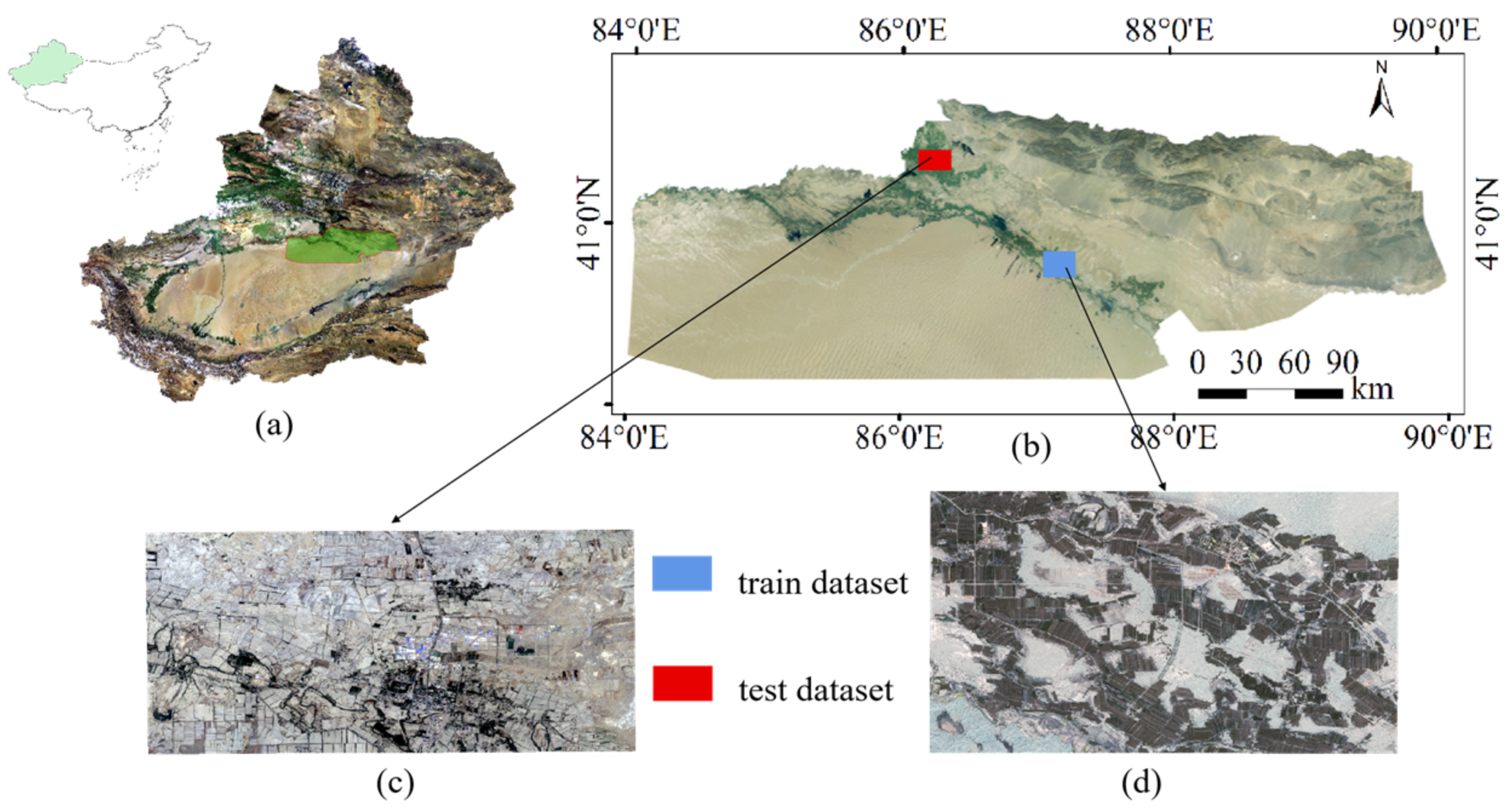
Figure 1. Overview map of the study area. (a) location of Yuli County in China as well as in Xinjiang; (b) range of GF-6 image acquisition; (c) training set; (d) test set.
Remotesensing 15 03283 g001
Figure 2. Multi-Unet network structure diagram.
Remotesensing 15 03283 g002
Figure 3. (a) Spatialwise attention guidance module, (b) channel attention guidance module, (c) “spatial-channel” attention guidance module.
Remotesensing 15 03283 g003
Figure 4. Classification results of the GF-6 data.
Remotesensing 15 03283 g004
Figure 5. Comparison of local area classification results of the pear tree dataset in Yuli County.
Remotesensing 15 03283 g005
Figure 6. The influence of different input band combinations on the classification accuracy of the Multi-Unet network.
Remotesensing 15 03283 g006
Figure 7. The part result of different models.
Remotesensing 15 03283 g007
Table 1. Accuracy comparison table of the Single module.
ModulePrecisionRecallIou
A: Spatialwise attention guidance module82.571.675.6
B: Channel attention guidance module83.872.577.5
C: “Spatial-channel” attention guidance module84.173.578.2
Table 2. Accuracy comparison table of the pear test dataset in Yuli County.
ModelInput SizePrecisionRecallF1Kappa
FCN8s256 × 25683.9759.9669.9668.77
512 × 51290.5356.4169.5168.39
SegNet256 × 25689.2560.8372.3571.28
512 × 51289.7359.1771.3170.22
U-Net256 × 25681.4375.4278.3177.31
512 × 51280.6272.2776.2275.14
Res-U-Net256 × 25686.2873.1179.1578.23
512 × 51269.0287.1677.0475.80
PSPNet256 × 25682.7376.9679.7478.82
512 × 51280.4076.7678.5476.01
RefineNet256 × 25675.3781.9478.5277.44
512 × 51275.7373.1774.4373.25
DeepLabv3+256 × 25688.2783.9786.0785.42
512 × 51279.1787.1282.9682.10
Multi-Unet256 × 25688.9589.5789.2688.74
512 × 51290.2876.6482.9082.15
Table 3. Comparisons of network efficiency and accuracy among the deep learning models.
FCN8sMulti-UnetU-NetRefineNetSegNetDeeplabv3+PSPNet101Res-U-Net
F176.3892.4590.5587.2286.9491.5588.287.45
IOU56.086.082.978.176.984.478.377.7
parameter3,050,7267,263,1437,847,1477,263,14331,821,70241,254,64666,239,013110,140,324
Model size (MB)11.6728.3430.0346.10121.63158.63253.4422.32
Disclaimer/Publisher’s Note: The statements, opinions and data contained in all publications are solely those of the individual author(s) and contributor(s) and not of MDPI and/or the editor(s). MDPI and/or the editor(s) disclaim responsibility for any injury to people or property resulting from any ideas, methods, instructions or products referred to in the content.