Article

Characteristics of Air Pollutant Distribution and Sources in the East China Sea and the Yellow Sea in Spring Based on Multiple Observation Methods

1
Key Laboratory for Aerosol-Cloud-Precipitation of China Meteorological Administration, Nanjing University of Information Science and Technology, Nanjing 210044, China
2
Polar and Marine Research Institute, College of Harbor and Coastal Engineering, Jimei University, Xiamen 361021, China
3
Emergency Management School, Nanjing University of Information Science and Technology, Nanjing 210044, China
*
Author to whom correspondence should be addressed.
Remote Sens. 2023, 15(13), 3262; https://doi.org/10.3390/rs15133262
Submission received: 31 March 2023 / Revised: 3 June 2023 / Accepted: 21 June 2023 / Published: 25 June 2023
(This article belongs to the Special Issue Air Quality Mapping via Satellite Remote Sensing)

Abstract

:
The composition of marine aerosol is quite complex, and its sources are diverse. Across the East China Sea (ECS) and the Yellow Sea (YS), multi-dimensional analysis of marine aerosols was conducted. The characteristics of carbonaceous aerosols and gaseous pollutants were explored through in situ ship-based observation, MERRA-2 reanalysis datasets and TROPOMI data from Sentinel-5P satellite. Black carbon (BC)’s average concentration is 1.35 ± 0.78 μg/m3, with high-value BC observed during the cruise. Through HYSPLIT trajectory analysis, sources of BC were from the northern Eurasian continent, the Shandong Peninsula, the ECS and Northwest Pacific Ocean (NWPO). The transport of marine sources like ship emissions cannot be ignored. According to the absorption Angstrom exponent (AAE), BC originates from biomass burning (BB) in the shortwave band (~370 nm) and from fossil fuel combustion in the longwave band (~660 nm). Organic carbon (OC), sulfate (SO42−) and BC report higher Angstrom exponent (AE) while dust and sea salt reveal lower AE, which can be utilized to classify the aerosols as being fine- or coarse-mode, respectively. OC has the highest AE (ECS: 1.98, YS: 2.01), indicating that anthropogenic activities could be a significant source. The process of biomass burning aerosol (BBA) mixed with sea salt could contribute to the decline in BBA’s AE. Ship emissions may affect the distribution of tropospheric nitrogen dioxide (NO2) in the ECS, especially during the COVID-19 pandemic. Tropospheric NO2 over the YS has the highest value (up to 12 × 1015 molec/cm2). Stratospheric NO2 has a ladder-like distribution from north to south, and the variation gradient was lower than that in the troposphere. Carbon monoxide (CO) accumulates in the south and east of the ECS and the east of the YS, while the variation over the eastern YS is relatively frequent. Seas near the Korean Peninsula have extremely high CO concentration (up to 1.35 × 10¹⁷ molec/cm2).

1. Introduction

Marine aerosols are some of the most important natural systems in the world, with important impacts on marine ecosystems, biogeochemical cycles and the global climate [1]. Marine aerosols can directly affect Earth’s radiation balance by absorbing and scattering solar radiation, namely direct radiation forcing. In addition, marine aerosols can drive climate change by participating in cloud condensation nuclei and ice nucleating particles, i.e., indirect radiation forcing. Through indirect radiation forcing, marine aerosols can alter the macro–microscopic properties of clouds, affecting precipitation cycles and possibly even triggering natural disasters such as flooding, drought and wildfires [2]. Atmospheric aerosols over the ocean are mainly influenced by local emissions or long-range transport. Long-range transport includes particle matter generated by biomass burning (BB), volcanic eruptions, deserts, etc., and sea salt from elsewhere such as the secondary generation of sulfate (SO42−), as well as gases such as nitrogen oxides (NOx) and sulfur dioxide (SO2) generated through anthropogenic activities [3,4,5,6]. Marine aerosol study not only helps to understand the extent of the impact of human activities on aerosol pollution, but also provides background data to support the transboundary transport of air pollutants [1,7,8,9].
As one of the most important air pollutants, black carbon (BC) absorbs solar radiation and has a strong warming effect on the climate, which is estimated to be the second most important carbon compound after carbon dioxide [10,11]. The aging of BC is worthy of attention due to its short lifetime. The aging process of BC aerosol in the atmosphere includes SO42−, organic carbon (OC) and secondary organic aerosol (SOA) in external and internal mixtures [12,13]. Compared with pure external mixing, the light absorption of BC can be increased by about 30–100% under effects of internal mixing with these components [14]. In addition to the aging, the uncertainty of BC absorption parameters (such as mass absorption cross-section, MAC) in the model is also caused by “using constant ambient relative humidity (RH) or not” and other factors [15]. The cumulative effect of this uncertainty will then be reflected in the output of large-scale and even global models [16]. Compared with land like the Indian Peninsula, most of the BC changes in the ocean basin of the Indian Ocean do not have significant systematic effects of diurnality in emissions. In East Asia, the concentrations of BC are underestimated by the multi-model ensemble mean (MMEM), even though MMEM shows better performance than most single-model predictions [17]. Moreover, the global model can accurately reproduce the BC change trend in North America and Europe, but greatly underestimates the BC change trend in Asia and the Arctic [18,19,20]. Therefore, it is necessary to conduct in situ observation and analysis of BC in Asia and Asian marginal seas to provide data for more accurate model prediction in future.
Nitrogen dioxide (NO2), one stable gaseous pollutant among NOx, cannot only form nitric acid rain when reacting with water (H2O) but also produces ozone (O3) under ultraviolet wavelengths in cloudless skies [21]. NO2 studies in China’s marginal seas mostly adopted fixed instrument observations [22,23] or model simulations, such as WRF-Chem [24,25], and the experimental areas were mostly the South China Sea (SCS) [23,24], Bohai Sea [25] or Hangzhou Bay [22]. In recent years, machine learning (ML) algorithms (such as random forest) have been utilized to analyze and predict NO2 with high accuracy [26]. However, due to the chaos and variability in the atmosphere, the ML model formed from one scenario may not be suitable for other scenarios, or the “generalization ability” will be low. Therefore, it is necessary to utilize remote sensing to observe NO2 over the East China Sea (ECS) and the Yellow Sea (YS), so as to explore the spatiotemporal variations on a larger scale.
East Asia is one of the regions with the highest aerosol concentration in the world, and its composition is complex and diverse, including desert dust, sea salt and carbon released through anthropogenic activities [27]. The YS, a semi-enclosed marginal sea in the Northwest Pacific Ocean (NWPO), is located between China and the Korean Peninsula. Adjacent to YS, the ECS is one of the three major marginal seas in Asia. For years, research on the chemical composition and source of marine aerosol over the ECS and the YS has mainly been based on ship-based observations [28,29,30,31] and island observations [32]. Previous studies have mainly focused on the source of dust [33], greenhouse gases (GHG) such as carbon monoxide (CO), methane (CH4), carbon dioxide (CO2) and nitrogen monoxide (N2O) [34], water-soluble ions such as non-sea salt sulfate (nss-SO42−), nitrate (NO3) and ammonium salt (NH4+) [35] and various trace elements [36]. Compared with those in pelagic areas, secondary inorganic aerosols, such as NO3, NO3 and NH4+, in winter over the ECS have high concentrations, and are mainly influenced by anthropogenic sources [37,38]. However, continuous online observation of BC along these oceanic regions is lacking. Therefore, an aethalometer was installed on board during a research cruise in April 2022, and BC concentrations over the ECS and the YS were observed and their correlations with variables (BB, temperature, etc.) were analyzed (shown in Section 3.1.1. and Section 3.1.2.). With the help of the HYSPLIT model, sources of BC were discussed based on air mass trajectories (Section 3.1.3). Combined with MERRA-2 reanalysis datasets, aerosol optical properties were also calculated and analyzed (Section 3.1.4). Moreover, the spatial distribution of NO2 in the troposphere (Section 3.2.1) and stratosphere (Section 3.2.2), and CO (Section 3.2.3) over the ECS and the YS, from 9 April to 26 April was presented through the use of a TROPOMI aerosol product. Through this study, the physical characteristics and distribution of carbonaceous aerosols and gaseous pollutants over China’s eastern marginal seas could be better understood.

2. Experimental Methods

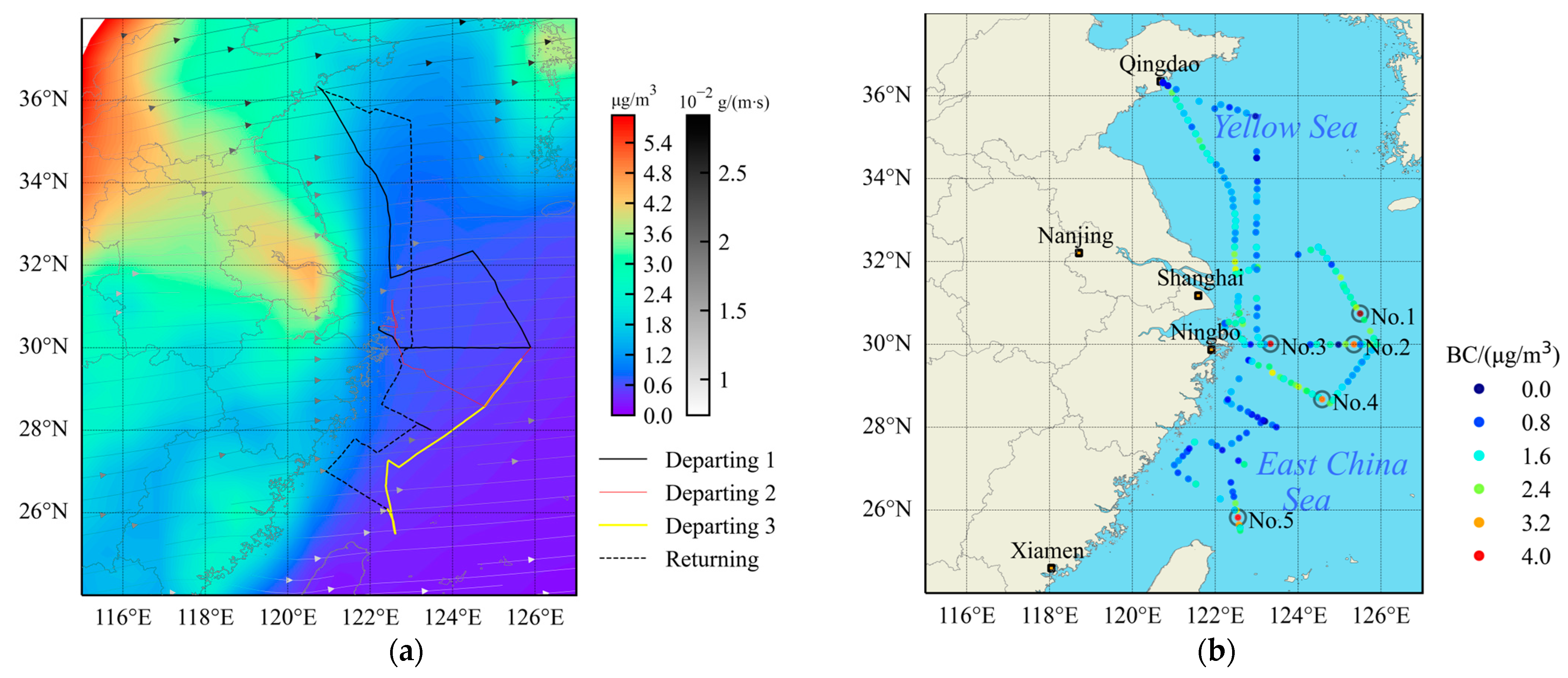
2.1. The Cruise Route

In this study, ship-based observations were investigated during the National Natural Science Foundation of China shared cruise to the ECS, which lasted approximately half a month during the boreal spring of 2022 (from 9 April to 26 April 2022), as shown in Figure 1a. This cruise was conducted onboard R/V “Xiang Yang Hong 18” by the First Institute of Oceanography, Ministry of Natural Resources, China.

2.2. In Situ Observation

BC mass concentration measurements were carried out using an aethalometer (Model AE33, Magee Scientific, Berkeley, CA, USA). It is worth noting that the BC measurement was conducted optically, which means that the BC concentration was derived from the particles’ light absorption, and hence we refer to the measured BC as equivalent black carbon (eBC) concentration. Due to the aethalometer only measuring the attenuation of light through the filter, a loading effect may have occurred, which may have caused an error. In order to solve this problem leading to discontinuity in the time series, AE33 introduces the “dual-spot” sampling technology [39], and uses the real-time compensation parameters of the correction algorithm of Virkkula [40] to correct the loading effect to improve data accuracy. In this paper, 880 nm eBC is referred to as the BC concentration. Moreover, we used a marine meteorological instrument to observe the meteorological parameters during the cruise, including the pressure, air temperature and wind speed, etc.

2.3. Observation Data Correction

Strong precipitation and strong wind will reduce BC concentration. Gupta et al. [41] found that high wind speed (>2 m/s) can promote dispersion and dilution, and then lead to a reduction in BC concentration in the atmosphere. To avoid the influence of the ship’s own emissions, we used corrected data recorded when the wind direction and speed relative to the ship’s course were within ±60° from the bow and >3 m/s, respectively. The same method was used to correct data in the 7th Chinese National Arctic Research Expedition [31].

2.4. AAE Calculation and AE Acquisition

The absorption Angstrom exponent (AAE) measures the wavelength dependence of BC’s light absorption and is inherent to the chemical variability in the components. Since AE33 can output BC of up to 7 bands (370, 470, 520, 590, 660, 880 and 950 nm), we calculated the BC AAE using the following calculation formula [42]:
σ abs ( λ 1 ) σ abs ( λ 2 ) = ( λ 1 λ 2 ) AAE
where σ abs represents the absorption coefficient, λ i ( i = 1 , 2 ) represents wavelengths and λ 1 < λ 2 . The σ abs at each wavelength were retrieved using the following formula [43]:
σ abs ( λ i ) = B C ( λ i ) MAC ( λ i )
where MAC are the mass absorption cross-section values which are used in the Aethalometer AE33, and are 18.47, 14.54, 13.14, 11.58, 10.35, 7.77 and 7.19 m2/g for the wavelengths of 370, 470, 520, 590, 660, 880 and 950 nm, respectively.
The Angstrom exponent (AE) is a parameter used to reflect particle size characteristics [44]:
τ λ = β λ α
where τ λ is the aerosol optical thickness at the wavelength λ . α represents the AE, and β is the turbidity parameter reflecting the cleanliness of the atmosphere. AE in April, 2022, as mentioned below, was accessed from MERRA-2 reanalysis data.

2.5. Satellite and Reanalysis Datasets

In the EUMETSAT Polar System (EPS) Second-Generation program, Sentinel-5P (S-5P) is a single-satellite, single-payload mission that serves as both a gap-filler and a preparation program for Sentinel-5. The TROPOspheric Monitoring Instrument (TROPOMI), which will monitor important atmospheric elements, such as O3, NO2, SO2, CO, CH4 and CH2O, and aerosol characteristics is the S-5P’s mission’s payload. The Ozone Monitoring Instrument (OMI) and the SCanning Imaging Absorption spectroMeter for Atmospheric Cartography (SCIAMACHY) are both TROPOMI’s ancestors [45]. We selected the TROPOMI data of 9, 14, 19 and 24 April 2022 (https://s5phub.copernicus.eu/dhus/#/home (accessed on 20 October 2022)) and analyzed the four-day mean distribution and anomaly distribution of each parameter.
The Modern-Era Retrospective analysis for Research and Applications, Version 2, (MERRA-2) provides data from 1980. MERRA-2 was the first long-term global reanalysis method to assimilate space-based observations of aerosols and reflect their interactions with other physical processes in the climate system. It was introduced to replace the original MERRA dataset because of the advances that were made in the assimilation system. The grid spacing is about 50 km [46]. The monthly averaged BC surface mass concentration, BC horizontal mass flux and AE in April 2022 were reached using the MERRA-2 Aerosol Diagnostics product (https://disc.gsfc.nasa.gov/datasets/M2TMNXAER_5.12.4/summary?keywords=MERRA-2 (accessed on 28 June 2022)), with a spatial resolution of 0.625° × 0.5° and a temporal resolution of one month.

2.6. Backward Trajectories

The Hybrid Single Particle Lagrangian Integrated Trajectory (HYSPLIT) model [47] of NOAA was applied to calculate the backward trajectories for the investigation of air mass sources and transport paths. Euclidean distance was used to cluster trajectories [48], helping to distinguish the polluted trajectories with a high value from a large number of trajectories. Then, the pollutant pathway could be estimated, which was associated with high-concentration clusters. In this study, the TrajStat plugin [49] was used to cluster the air mass trajectories at each point and calculate the proportion of various trajectories to the total trajectories.
Based on the Global Data Assimilation System (GDAS) meteorological data from March to April 2022 (ftp://ftp.arl.noaa.gov/pub/archives/gdas1 (accessed on 16 May 2022)) and the MeteoInfoMap software [50], the HYSPLITY model was used to simulate the backward trajectory of the selected atmospheric pollutants. In this study, the model operation height was set at 50 m and the backward simulation time was 7 days, considering that the lifetime of BC is about 4–12 days [51]. The simulation was conducted at 00:00, 06:00, 12:00 and 18:00 (UTC) every day from 9 April to 26 April.

3. Results and Discussion

3.1. Carbonaceous Aerosols
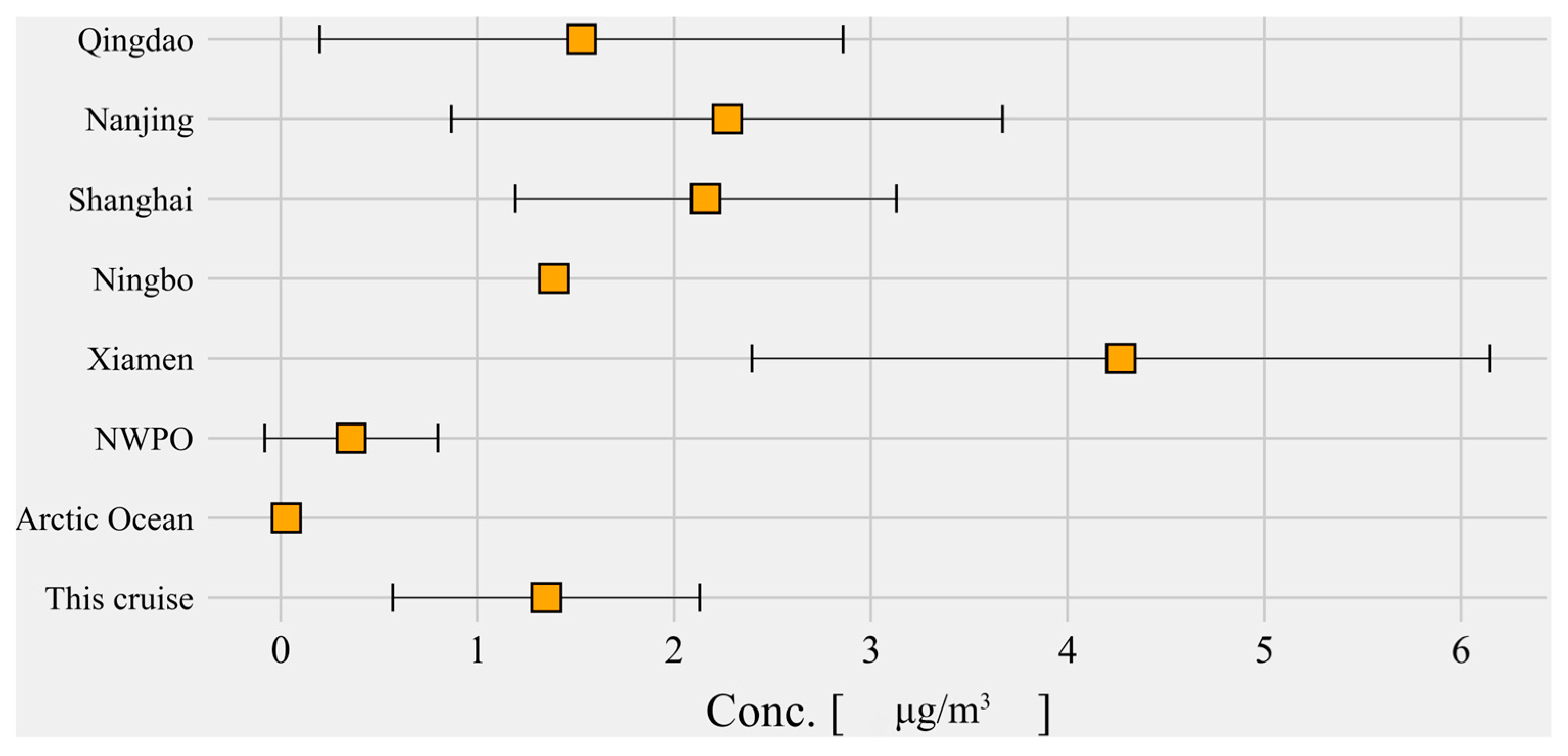
3.1.1. BC Variation

As shown in Figure 1a, this voyage started from Qingdao, China, and passed through the Yellow Sea and the East China Sea. In April 2022, there was a high BC value (>4.8 μg/m3) in the west of Shandong Province and southern Jiangsu Province in China. The BC horizontal mass flux expressed prevailing westerly winds and larger flux occurred in the north, indicating that the continent was one of the main BC sources in marginal seas and coast. Significant concentration differences were shown between the marginal sea and land, most notably in the southern ECS (Figure 1a). As shown in Figure 1b, the BC concentrations in the ECS were almost all less than 1.2 μg/m3. There are high BC values (>3.4 μg/m3) in the middle of the Yellow Sea, the estuary of the Yangtze River, the waters near 30°N and the northeast of Taiwan Island.
The corrected data can eliminate the impact of the ship’s own emissions on the observation as much as possible, and can better describe the change trend in BC concentration (Figure 2). Since Point No. 5 is just at the dividing point between departing and returning (see Figure 1b for details), the cruise can be divided into two sections for analysis based on Point No. 5. In the previous period, obvious abnormally high points were filtered. After Point No. 5, the BC concentration showed a downward trend, and stabilized at 0.6 μg/m3 after 21 April. The abnormally high value of 23–24 April was filtered based on the correction. The following discussions are based on corrected data.
The previous ECS and terrestrial observation results were selected to compare and analyze the temporal and spatial variations in BC concentration distribution (Table 1 and Figure 3). Table 1 shows the basic information of previous observations, including Qingdao (36.350°N, 120.680°E), Nanjing (32.205°N, 118.715°E), Shanghai (31.180°N, 121.590°E), Ningbo (29.870°N, 121.910°E) and Xiamen (118.050°E, 24.600°N), as well as two cruises in the NWPO and the Arctic Ocean. Moreover, Figure 3 revealed that BC concentrations during this cruise (1.35 ± 0.78 μg/m3) varied within concentrations of the previous land and oceanic observations. In spring, BC concentrations in Qingdao, Nanjing and Shanghai differed. On the one hand, compared with the Nanjing observation site, which is far away from the city center, the Qingdao site has the highest observation height and is not easy to be affected by the BC emission at the bottom; on the other hand, 2020 was a time when China’s COVID-19 situation was serious and air pollutant emissions were relatively low [52]. The BC concentration in the Ningbo station is the closest to this cruise value, as the two studies were closer geographically. Due to a far distance from the land and a less-direct source, the BC concentration of the NWPO and the Arctic Ocean is significantly lower than that of land and coast, but also much lower than our cruise results.

3.1.2. The Relationship between BC and Other Variables

The AE33 Aethalometer’s seven wavelengths enable the instrument to calculate a percentage of BB contribution to BC using an algorithm developed by Sandradewi et al. [58], which can be used to analyze the origin and formation of BC. Using the benefits of AE33′s seven wavelengths, the algorithm calculates the difference in absorption in the ultraviolet wavelengths (almost entirely by brown carbon (BrC)) and the near infrared wavelengths (only by BC). The correlation between BC concentration and BB contribution (%) was analyzed in the ECS (latitude < 32.5°N) and YS (latitude ≥ 32.5°N). Overall, the correlation between the BC and BB contributions was negative (R2 = 0.177, p < 0.01), and most BCs were in areas with a BB contribution value of < 40% (Figure 4), indicating that BC from BB in the YS and ECS was lower than that from other sources, such as fossil fuel combustion. The two fitting lines are nearly parallel and the ECS one has a larger intercept, indicating that the BC concentration level was higher over the ECS with the same BB contribution. Compared to ECS (R2 = 0.145, p < 0.01), the BC and BB ratios are more correlated in the YS (R2 = 0.273, p < 0.01). The BB contribution decreased with an increasing BC concentration, which may have resulted from two potential factors: (1) The contribution of fossil fuel combustion to BC increased with an increasing BC concentration. Fossil fuels contribute more than BB to BC concentrations in coastal cities in southern China in the spring and autumn [59]. These fossil fuels include coal and liquid fuels. Among all forms of fossil fuel combustion, coal combustion contributes a lot to BC in northeast China [60]. (2) BC emitted from BB to the eastern marginal seas decreased with increasing total BC. Research found that biomass burning aerosol (BBA) originated from South Asia could be a result of long-range transport and influence the Pacific Ocean. However, compared to the land, this BBA has a low volume fraction of BC [61].
Although the ECS is adjacent to the YS, meteorological conditions differ from each other, mainly reflected in the atmospheric temperature, pressure, wind speed and RH. This may be related to latitudinal differences, sea–land transport or coastal terrain. The correlation and significant level between BC concentrations and meteorological parameters were analyzed and the influencing factors on BC concentration in the eastern marginal seas of China were investigated. As shown in Figure 5, the correlations between BC and different meteorological parameters in two oceanic regions vary considerably. The positive correlation between BC and wind speed (R2 = 0.230, p < 0.01), pressure (R2 = 0.203, p < 0.01) over the YS and temperature (R2 = 0.026, p < 0.05) over the ECS is found during the study period. The middle–lower reaches of the Yangtze River plain and North China plain are located on the west side of the YS, where anthropogenic activities are frequent. Peak emissions from forest fires normally occur in the spring of northeastern China [62], while a great contribution from coal combustion (CC) is non-negligible as well [60]. Horizontal mass flux also indicated that strong westerly winds could transport CC-generated BC to the YS (Figure 1a). In the northeast of China, a positive correlation between aerosol optical depth (AOD) and surface RH, and a negative correlation between AOD and surface wind speed or sea level pressure, were found from 1980 to 2017 [63]. As AOD means light-absorbing capacity of aerosol and can partly represent BC concentration, it implies that BC’s correlations with RH and pressure differ between the northern China and nearby marginal seas.

3.1.3. Backward Trajectories of BC

In the sampling route, several high-value points (Nos. 1–5) during the cruise were selected and the 7-day air mass backward trajectory was analyzed. Western China (including the Loess Plateau, the Taklimakan Desert and the deserts in Qinghai Province) and the Gobi Desert are recognized as the main sources of the dust arriving in the ECS, based on previous studies [33,36]. Due to the different lifetime and scale of various sources, BC may have different sources, and the proportion of each source varies greatly. Briefly, backward trajectory analysis finds that in addition to the common inland sources, maritime shipping emissions and coastal anthropogenic sources are potential BC sources. As shown in Figure 6a–c, the backtrack sources of Point Nos. 1–3 are relatively similar, which can be divided into Russian sources, ECS (or YS) local sources and NWPO sources. Among them, the Russian source of No. 1 can be subdivided into the Siberian continental source (15.28%) and the Baikal Lake source (36.11%). In fact, BB from Siberia does increase the BC concentration in remote oceans such as the Arctic Ocean and the Bering Sea [64]. The proportion of the NWPO source is smaller than that of the Baikal Lake source, followed by the ECS source, and the Siberian source is the lowest. Compared with Point No. 2, where the proportion of backward track sources is evenly distributed, No. 3 focuses more on Russia, with a higher proportion (43.06%), followed by the ECS sources (33.33%) and the NWPO sources (23.61%). For Point No. 4 (Figure 6d), pollutants come from Russia (38.89%), the eastern Shandong Peninsula of China (18.06%) and the NWPO (total 43.06%, including offshore Japan (27.78%) and the remote NWPO (15.28%)). The No. 5 sampling point is close to Taiwan Province and is at the beginning of the return route (Figure 6e). Its trajectories near Lake Baikal in Russia and Northeast China account for 33.33% and 18.06%, respectively. The other two oceanic sources belong to the Northwest Pacific, consisting of offshore Japan (26.39%) and the remote NWPO (22.22%). This implies that the NWPO might be a non-negligible source of the air pollutant mass. Frequent maritime trade has increased the number of ships in the last decade [65]; thus, ship emissions have led to an increase in BC over remote oceans (like the Southern Ocean) [66]. Moreover, fossil fuel emissions, as the main form of ship emissions, affect aerosol components in the marine atmosphere [67].
Comparing these three points with the highest BC value (Point Nos. 1, 3 and 5, corresponding to Figure 6a,c,e, respectively), it is found that two of them (Point Nos. 3 and 5) are closer to the shore, but the impact of the potential BC from the transport from marine air mass is more than 48%, indicating that in spring, the BC concentration in the eastern sea area of China is affected to some extent by the transport of marine sources, such as ship emissions. A previous study revealed that the BC mass concentration increased as a result of maritime shipping, with an estimated 10% increase [68]. In the Mediterranean atmosphere, for example, the contributions of ship emissions for BC close to the main shipping routes were confirmed to range from 10% to 50% [69].

3.1.4. Optical Properties

AE or AAE are important parameters reflecting aerosol properties, providing vital messages about aerosol particle size and effective radius, as well as the formation and growth mechanisms [70,71]. Higher AE values can be used to depict fine aerosol particles, which are often caused through anthropogenic activities, while lower AE values can be used to describe coarse-mode aerosol particles like dust particles [72,73,74,75]. AAE could reflect the source of BC. Previous studies have indicated that when BC mainly comes from BB, the AAE value is about 2; when BC mainly comes from fossil fuel combustion, the AAE value is about 1 [58,76,77].
Calculating the AAE with a fixed λ 1   (see Equation (1)), it is found that the larger the λ 2 , the smaller the AAE value (Table 2). Compared with inland Asia [43], the AAE calculated by the YS and the ECS in this experiment is higher in the same wavelength range ( λ 2 λ 1 ). In the same season, the AAE of the YS and the ECS at a low λ 1 is higher than that of ships near the South China Sea (SCS), but the AAE of BB over the SCS is higher and more stable [78]. The AAE measured and calculated on land and sea basically conforms to the rule of AAE 370 520 > AAE 370 950   >   AAE 660 950 . Longwave AAE is close to one, indicating that BC is mainly derived from fossil fuel combustion. AAE in the shortwave band is close to two, which implies that BB is significant. In addition to the common absorbable aerosols such as BC and sand dust, BrC, with a high AAE value [79], could be a factor to raise the AAE value over the ECS region, due to the influence of East Asia continent transport in spring [80].
AE was directly obtained from the MEERA-2 product, which could be utilized to analyze the average distribution within the designated YS (33–37°N, 120–126.25°E) and ECS (25–32°N, 120–126.87°E) range (Figure 7). On the whole, total aerosol AE decreases from land to sea, but the AE distribution of different variables (BC, dust, organic carbon (OC), sea salt, SO42− and total aerosol) is quite different (Figure 7). OC, SO42− and BC reported higher AE values, while dust and sea salt revealed lower AE values, which could be utilized to classify the aerosols as being fine- or coarse-mode, respectively. The high value of the AE of BC and dust is found in the NWPO direction, and a relatively low value emerged in the middle of the ECS. Considering that there are densely populated lands on the east and west sides of the ECS, this distribution shows that BC generated through anthropogenic activities is one of the important factors affecting the radiation budget of the ECS. The high AE of OC, sea salt and SO42− is located in the northwest of the YS and the north of the ECS, where the YS has the highest value in the sea area near the south of Shandong Peninsula, China. In Table 2, SO42− is also an important variable that affects the optical properties of aerosols over the ECS and the YS, with a mean AE value of 1.75 in the YS region and 1.65 in the ECS region, and even exceeds BC (ECS: 1.45, YS: 1.44). The higher AE value indicates that the concentration of SO42− is relatively high and may be related to combustion sources. It is known that when both BB and industrial emissions influenced the observation sites in Asia, concentrations of SO42− (in chemical form, like (NH4)2SO4) increased [81]. For the AE value of SO42−, the gap between the YS and the ECS has a maximum of 0.1. OC has the highest AE value in the above two sea areas (YS: 2.01, ECS: 1.98), which means that anthropogenic emissions can be a significant source of OC over the ECS and the YS. BBA over the ocean usually has a lower AE [61], reflecting the particle size growth of BBA during the aging process. The marine environment is rich in sea spray aerosol, which consists of coarse particles with a relatively lower AE (shown in Figure 7). Combined with the fact that the source of BC from the ocean accounted for a significant portion of the entire source, the process of BBA mixed with sea salt could contribute to the decline in BBA’s AE.
Table 2. Information on absorption Angstrom exponent (AAE) or Angstrom exponent (AE) in different studies.
LocationsTimeAAE or AESource
Beijing, China2005–2017 AAE 675 (Annual) AE 440 870   (Spring) AE 440 870   (Summer)[82]
0.00–1.701.19 ± 0.210.75 ± 0.33
AE 440 870 (Autumn) AE 440 870   (Winter)
0.85 ± 0.170.85 ± 0.32
September–November 2015 AAE 370 950 AAE 370 520 AAE 660 950 [43]
Lulang, China1.12 ± 0.371.34 ± 0.470.97 ± 0.31
Lhasa, China1.04 ± 0.091.12 ± 0.150.94 ± 0.07
Sanya, SCSApril–May 2017 AAE ship AAE biomass AAE vehicle [78]
1.06 ± 0.031.75 ± 0.060.96 ± 0.06
Okinawa, Japan2006–2008 AAE all AAE only   spring AAE excluding   spring [80]
3.06 ± 1.003.34 ± 0.861.94 ± 0.74
YS+ECS, ship-based9–26 April 2022 AAE 370 950 AAE 370 520 AAE 660 950 This study
1.32 ± 0.421.73 ± 0.070.92 ± 0.25
1–30 April 2022 AE BC  1 AE dust AE OC AE sea   salt AE SO 4  2 AE total
YS, MERRA-21.44−0.062.010.031.750.99
ECS, MERRA-21.45−0.051.980.021.651.01
1 MERRA-2 AEs represent “Angstrom parameter [470–870 nm]”. 2 “SO4” means sulfate (SO42−).

3.2. Gaseous Pollutants

3.2.1. NO2 in the Troposphere

Human activities are the main source of NO2 in the troposphere, accounting for about two thirds of the total NO2 emissions, including the emissions from power generation, transportation and BB in the process of industrialization [83]. In the stratosphere, however, one main source of NO2 is NOx generated by the oxidation of N2O in the middle of the stratosphere, considering that NOx is the catalyst of O3 depletion. The other sources include lightning high-voltage discharge in nature, anthropogenic emissions like aircraft and spacecraft and the exchange with tropospheric NO2 caused by atmospheric circulation or convection. In particular, the effect of convection and circulation may affect the observation results of satellite remote sensing. As shown in Figure 8, Figure 9 and Figure 10, the left side is the 4-day average value, and the four pictures on the right side are the average value subtracted from the satellite-observed value on 9,14, 19, 24 April. In Figure 8, in the troposphere, the coverage rate of the NO2 column concentration data in the area of concern is still considerable after quality screening. The high-value areas of NO2 column concentration are concentrated in the vicinity of (26–28°N, 32–34°N) and 121°30′E. The high-concentration values lack spatial continuity. The overall NO2 concentration over the ECS shows an increasing trend, while the NO2 over the South Yellow Sea (30–35°N, 118.5–125.5°E) suddenly increased on the 24 April (Figure 8b–e). Previous research showed that upper tropospheric ozone (O3) increases with NOx emissions, whereas policies to reduce surface NOx emissions also reduce upper tropospheric O3 during the Asian summer monsoon [84]. NO2 on the surface may not only affect NO2 in the upper troposphere via convection, but may also affect other compositions in the upper troposphere.
Compared with the relevant studies on the ECS nearshore before the pandemic [85], NO2 in the troposphere is more prominent in the high-value part (>9 × 10¹⁵ molec/cm2) in this study. On the one hand, the accumulation of ships in ports is one of the reasons. On the other hand, non-terrestrial sources are also some of the reasons that affect the change in NO2 concentration over the ECS surface. The non-terrestrial source of NO2 is represented by ship emissions. During the lockdown of Wuhan in the 2020 epidemic, the concentration of NO2 in the inland decreased significantly, with that in the Wuhan and Beijing–Tianjin–Hebei (BTH) regions decreasing by 54% and 83%, respectively [86]. However, there was no sign then that a significant NO2 change happened over the oceanic region. In theory, the sea area affected by the westerly wind transport should present a difference in emissions before and after the lockdown. In addition, during the study period, Shanghai, a city near the ECS, took measures to restrict anthropogenic activities for controlling the spread of the pandemic. This further shows that non-terrestrial sources can also lead to an increase in NO2 concentration.

3.2.2. NO2 in the Stratosphere

Compared with NO2 in the troposphere, NO2 distribution in the stratosphere was more regular and the variation gradient was not significant (from ~2.25 to ~3.45, shown in Figure 9a). For the mean value, the overall concentration level increases from south to north. In the area south of 31°N, the NO2 concentration near 123°E would be lower than that in other areas at the same latitude. To the north of 31°N, the zonal distribution was gradually uniform, and the marginal seas near the Shandong Peninsula of China had prominent high-value areas. It is shown in Figure 9b–e that temporal variations were reflected in the sea, land, longitude, latitude and specific sea areas. In the west direction, the region could be divided into north and south sections by 34°N for analysis. To the north of 34°N, the NO2 variation was centered in the eastern sea area of Shandong Peninsula, China, and reached the maximum on the 14 April. In the area south of 34°N, the concentration of NO2 in most areas was higher than the average value on the 9 April, and there were abnormally high values at the junction of Jiangsu Province and Anhui Province and the sea area near Shanghai. On the 14 April, taking the central sea area of the ECS as the center, the concentration of NO2 dropped sharply and this was the lowest value of NO2 anomaly in 4 days. It is noteworthy that the negative value area near 28°N of the stratosphere corresponds to the positive value area of the troposphere. Since this area is far from the land, it can be attributed to the vertical exchange under the influence of convection or turbulence on the sea surface. On the 19 April, the NO2 concentration in the southern part of the YS and the ECS rose again to above the average value. The high-value area was similar to that on the 9 April, with a higher anomaly. On the 24 April, except for that in the YS, the concentration of NO2 in the ECS was higher than that of the average value, and the high-value area of the NO2 anomaly was moving eastward compared with the low-value area on the 14 April. All in all, the variation in NO2 in the stratosphere is slighter but more frequent than that in the troposphere.

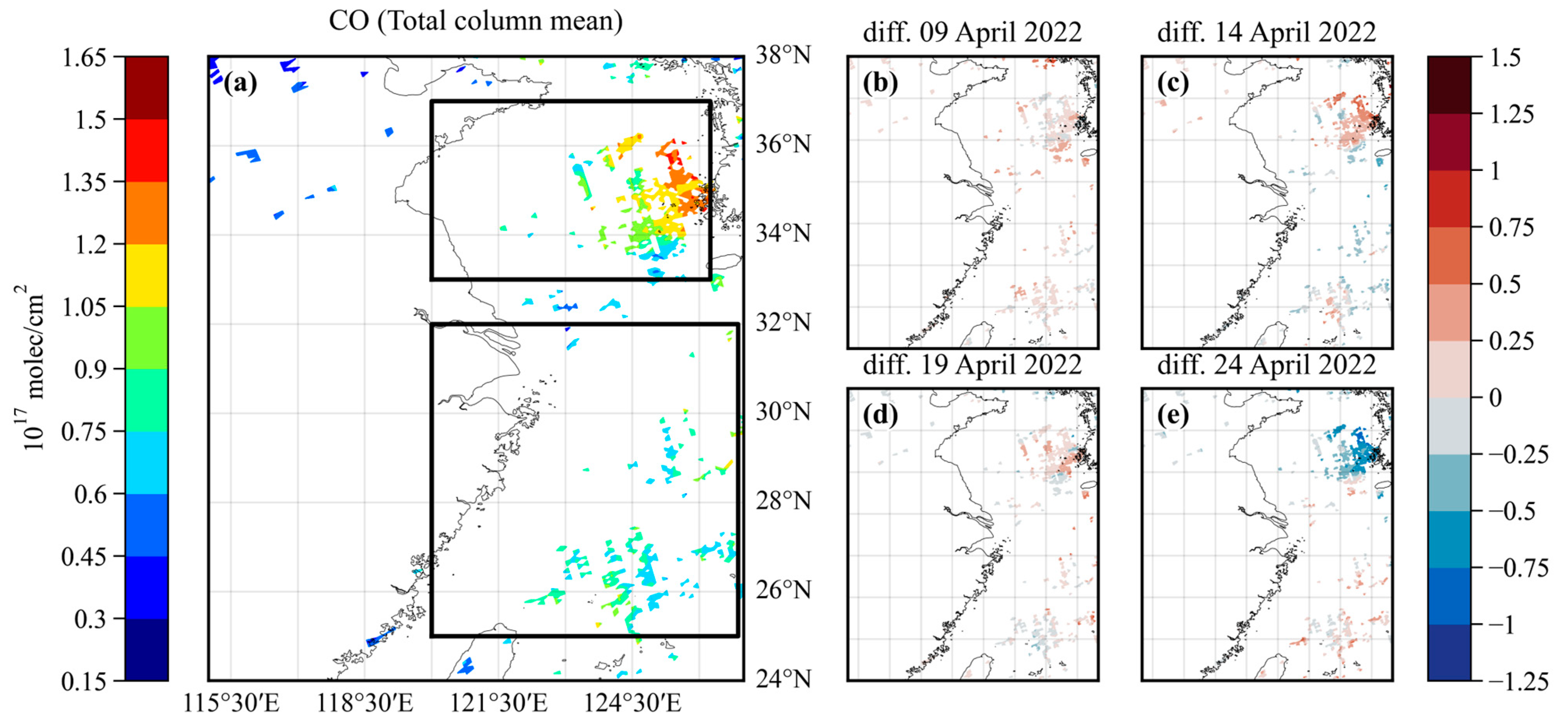
3.2.3. CO in the Total Column

One main source of CO emissions is BB [87]. CO emissions occur from coal combustion, especially when the flame is extinguished after coal loading [88]. CO over the ocean surface is slightly different to that from the land. CO in surface seawater mainly comes from photochemical generation [89], rainwater [90] and marine organisms [91], as well as emissions from the ocean to the atmosphere [92]. For the CO column concentration (Figure 10a), the high values are mainly in the south and east of the ECS, and in the east of the YS. The sea area near the Korean Peninsula has extremely high values of CO, and the lowest value is in the offshore area in the southwest corner of the Korean Peninsula.
From the perspective of temporal variation (Figure 10b–e), the highest value for CO appeared at the intersection between the ECS and the YS on 24 April. The variation trend in the CO concentration of the study aera was consistent with the nearby YS area and ECS, whereby both of which increased in the next two days. On the contrary, the YS area to the west of the Korean Peninsula dropped to the lowest value on the final day. CO in the South Yellow Sea was discovered to exhibit apparent diurnal variation [93], while there is less diurnality over the YS because the air masses tend to stay there [34]. The unfixed sampling time of the Sentinel-5p satellite orbit in the same area could help to explain CO distribution in the YS which is affected by the diurnal difference and local meteorological conditions. It is suggested that future CO analysis in this area can be carried out “in diurnal or not” or “in clear-sky atmospheres or not” for more accurate analysis.
As a product of incomplete combustion, offshore CO can also be transported from land to sea, the same as BC and NOx. Over the ECS and the YS, due to the vast area and inconvenient installation of instruments, it is rare to use ship-based observations to collect data. So, remote sensing technology can be utilized. We analyzed the common gaseous pollutants over the ECS and the YS, which is conducive to the study of the characteristics of the “land–sea” exchange and “air–sea” exchange of marine air pollutants. In the future, advanced research could be conducted on the “air–sea” exchange of pollutants over the China marginal seas, in terms of aspects like dry deposition flux.

4. Conclusions

This study utilized the AE33 Aethalometer and Sentinel-5P satellite as the observation measurements, and used ship-based in situ BC observation data, MERRA-2 reanalysis data and TROPOMI aerosol column concentration data, taking the ECS and the YS as the research objects, to analyze the spatial and temporal variation characteristics and optical properties of carbonaceous aerosols and gaseous pollutants in the eastern marginal seas of China in spring. We have revealed the current situation of air pollution over the ECS and the YS in spring, and provided the scientific basis for the government to establish air pollution control policies. Based on the processes above, we have the following conclusions:
(1)
Compared with the BC observation on the land near the ECS, the in situ ship-based data (1.35 ± 0.78 μg/m3) are lower, but higher than the previous NWPO data. Concentration accumulation may have occurred at some repeatedly passing points in the ship route, which may have affected the analysis of pollution causes.
(2)
The backward trajectories of BC show that the main air mass sources in spring are the northern Eurasian continent, Shandong Peninsula, the ECS and the NWPO. The BC concentration in the eastern marginal seas of China is influenced by the transport of marine sources like ship emissions. Attention should be paid to the remote NWPO and the interior of the ECS.
(3)
The calculated AAE during the cruise conforms to the rule of AAE 370 520 > AAE 370 950 > AAE 660 950 . BC is more likely to originate from BB in the shortwave band (~370 nm) and from fossil fuel combustion in the longwave band (~660 nm). Generally, OC, SO42− and BC reported higher AE values, which indicates fine-mode aerosols, while dust and sea salt revealed lower AE values, which could be utilized to classify the aerosols as being coarse-mode. OC’s high AE means that anthropogenic emissions can be a significant source of OC. The process of BBA mixed with sea salt could contribute to the decline in BBA’s AE.
(4)
The emissions of ships accumulated in offshore ports and non-terrestrial pollutants affect the distribution of tropospheric NO2 in the ECS. Tropospheric NO2 over the ECS and the YS shows an increasing trend. Tropospheric NO2 over the YS has the highest value (up to 12 × 1015 molec/cm2).
(5)
Stratospheric NO2 is distributed along the north and south, with the maximum value in the marginal seas near the Shandong Peninsula of China (up to 3.3 × 10¹⁵ molec/cm2). The variation gradient in NO2 was lower in the stratosphere compared to that in the troposphere, especially in the southern YS. It cannot be ignored that there is potential vertical exchange of NO2 over the ECS in spring.
(6)
CO mainly accumulates in the south and east of the ECS and the east of the YS, while variation over the eastern YS is relatively frequent. The area near the Korean Peninsula over the YS has extremely high values (up to 1.35 × 10¹⁷ molec/cm2).

Author Contributions

Conceptualization, G.X. and Y.W.; methodology, L.C., G.X. and Y.W.; software, Y.W.; validation, Y.W. and K.C.; formal analysis, Y.W.; investigation, Y.W.; resources, G.X. and K.C.; data curation, Y.W.; writing—original draft preparation, Y.W. and G.X.; writing—review and editing, Y.W. and L.C.; visualization, Y.W.; supervision, L.C. and G.X.; project administration, Y.W., G.X. and K.C.; funding acquisition, G.X. All authors have read and agreed to the published version of the manuscript.

Funding

This research was funded by the National Natural Science Foundation of China, grant number 42006190.

Data Availability Statement

TROPOMI data were downloaded from Sentinel-5P Pre-Operations Data Hub (https://s5phub.copernicus.eu/dhus/#/home, accessed on 30 March 2023). GADS meteorological data were downloaded from ftp://ftp.arl.noaa.gov/pub/archives/gdas1, accessed on 30 March 2023. BC surface mass concentration and Angstrom parameters from MERRA-2 were downloaded from https://doi.org/10.5067/FH9A0MLJPC7N, accessed on 30 March 2023.

Acknowledgments

Data acquisition and sample collections were supported by the Planning Open Research Cruise for the East China Sea study of 2021, with a special focus on cross-shelf carbon transport (cruise no. NORC2022-02+NORC2022-301), funded by the Shiptime Sharing Project of the National Natural Science Foundation of China. This cruise was conducted onboard R/V “Xiang Yang Hong 18” by The First Institute of Oceanography, Ministry of Natural Resources, China. We appreciate the great help from all of the crews of R/V “Xiang Yang Hong 18”. The authors would like to thank the following institutions for datasets: NASA Global Modeling and Assimilation Office (GMAO) for MERRA-2, The Royal Netherlands Meteorological Institute (KNMI) and SRON for TROPOMI data on the ESA Sentinel-5 Precursor. Thanks to Yuying Wang for helping with the installation of the instruments onboard. Thanks to Yaqiang Wang from the Chinese Academy of Meteorological Sciences for the MeteoInfoMap software (https://github.com/meteoinfo, accessed on 30 March 2023) used to complete HYSPLIT analysis. Thanks to Yongjie Huang (IAP/CAS) for providing the map database (https://github.com/huangynj/Python-Chinamap.git, accessed on 30 March 2023). Thanks to Alejandro Keller for the useful code reference for this article on processing in situ observed BC data from AE33 Aethalometer (https://github.com/alejandrokeller/aethalometer.git, accessed on 30 March 2023).

Conflicts of Interest

The authors declare no conflict of interest.

References

  1. O’Dowd, C.D.; de Leeuw, G. Marine Aerosol Production: A Review of the Current Knowledge. Philos. Trans. R. Soc. A 2007, 365, 1753–1774. [Google Scholar] [CrossRef] [PubMed]
  2. Andreae, M.O.; Rosenfeld, D. Aerosol–Cloud–Precipitation Interactions. Part 1. The Nature and Sources of Cloud-Active Aerosols. Earth-Sci. Rev. 2008, 89, 13–41. [Google Scholar] [CrossRef]
  3. Su, Y.; Han, Y.; Luo, H.; Zhang, Y.; Shao, S.; Xie, X. Physical-Optical Properties of Marine Aerosols over the South China Sea: Shipboard Measurements and MERRA-2 Reanalysis. Remote Sens. 2022, 14, 2453. [Google Scholar] [CrossRef]
  4. Tian, M.; Li, H.; Wang, G.; Fu, M.; Qin, X.; Lu, D.; Liu, C.; Zhu, Y.; Luo, X.; Deng, C.; et al. Seasonal Source Identification and Formation Processes of Marine Particulate Water Soluble Organic Nitrogen over an Offshore Island in the East China Sea. Sci. Total Environ. 2023, 863, 160895. [Google Scholar] [CrossRef] [PubMed]
  5. Duflot, V.; Bègue, N.; Pouliquen, M.-L.; Goloub, P.; Metzger, J.-M. Aerosols on the Tropical Island of La Réunion (21°S, 55°E): Assessment of Climatology, Origin of Variability and Trend. Remote Sens. 2022, 14, 4945. [Google Scholar] [CrossRef]
  6. Wang, L.; Mačak, M.B.; Stanič, S.; Bergant, K.; Gregorič, A.; Drinovec, L.; Močnik, G.; Yin, Z.; Yi, Y.; Müller, D.; et al. Investigation of Aerosol Types and Vertical Distributions Using Polarization Raman Lidar over Vipava Valley. Remote Sens. 2022, 14, 3482. [Google Scholar] [CrossRef]
  7. Brooks, S.D.; Thornton, D.C.O. Marine Aerosols and Clouds. Annu. Rev. Mar. Sci. 2018, 10, 289–313. [Google Scholar] [CrossRef]
  8. Carpenter, L.J.; Fleming, Z.L.; Read, K.A.; Lee, J.D.; Moller, S.J.; Hopkins, J.R.; Purvis, R.M.; Lewis, A.C.; Müller, K.; Heinold, B.; et al. Seasonal Characteristics of Tropical Marine Boundary Layer Air Measured at the Cape Verde Atmospheric Observatory. J. Atmos. Chem. 2010, 67, 87–140. [Google Scholar] [CrossRef]
  9. Xu, W.; Ovadnevaite, J.; Fossum, K.N.; Lin, C.; Huang, R.-J.; Ceburnis, D.; O’Dowd, C. Sea Spray as an Obscured Source for Marine Cloud Nuclei. Nat. Geosci. 2022, 15, 282–286. [Google Scholar] [CrossRef]
  10. Fierce, L.; Onasch, T.B.; Cappa, C.D.; Mazzoleni, C.; China, S.; Bhandari, J.; Davidovits, P.; Fischer, D.A.; Helgestad, T.; Lambe, A.T.; et al. Radiative Absorption Enhancements by Black Carbon Controlled by Particle-to-Particle Heterogeneity in Composition. Proc. Natl. Acad. Sci. USA 2020, 117, 5196–5203. [Google Scholar] [CrossRef]
  11. Bond, T.C.; Doherty, S.J.; Fahey, D.W.; Forster, P.M.; Berntsen, T.; DeAngelo, B.J.; Flanner, M.G.; Ghan, S.; Kärcher, B.; Koch, D.; et al. Bounding the Role of Black Carbon in the Climate System: A Scientific Assessment: BLACK CARBON IN THE CLIMATE SYSTEM. J. Geophys. Res. Atmos. 2013, 118, 5380–5552. [Google Scholar] [CrossRef]
  12. Adachi, K.; Buseck, P.R. Internally Mixed Soot, Sulfates, and Organic Matter in Aerosol Particles from Mexico City. Atmos. Chem. Phys. 2008, 8, 6469–6481. [Google Scholar] [CrossRef]
  13. Sharma, N.; China, S.; Bhandari, J.; Gorkowski, K.; Dubey, M.; Zaveri, R.A.; Mazzoleni, C. Physical Properties of Aerosol Internally Mixed With Soot Particles in a Biogenically Dominated Environment in California. Geophys. Res. Lett. 2018, 45, 11473–11482. [Google Scholar] [CrossRef]
  14. Cappa, C.D.; Onasch, T.B.; Massoli, P.; Worsnop, D.R.; Bates, T.S.; Cross, E.S.; Davidovits, P.; Hakala, J.; Hayden, K.L.; Jobson, B.T.; et al. Radiative Absorption Enhancements Due to the Mixing State of Atmospheric Black Carbon. Science 2012, 337, 1078–1081. [Google Scholar] [CrossRef]
  15. Liu, S.; Aiken, A.C.; Gorkowski, K.; Dubey, M.K.; Cappa, C.D.; Williams, L.R.; Herndon, S.C.; Massoli, P.; Fortner, E.C.; Chhabra, P.S.; et al. Enhanced Light Absorption by Mixed Source Black and Brown Carbon Particles in UK Winter. Nat. Commun. 2015, 6, 8435. [Google Scholar] [CrossRef] [PubMed]
  16. Hopke, P.K. An Introduction to Receptor Modeling. Chemom. Intell. Lab. Syst. 1991, 10, 21–43. [Google Scholar] [CrossRef]
  17. Chen, L.; Gao, Y.; Zhang, M.; Fu, J.S.; Zhu, J.; Liao, H.; Li, J.; Huang, K.; Ge, B.; Wang, X.; et al. MICS-Asia III: Multi-Model Comparison and Evaluation of Aerosol over East Asia. Atmos. Chem. Phys. 2019, 19, 11911–11937. [Google Scholar] [CrossRef]
  18. Tian, P.; Zhang, L.; Ma, J.; Tang, K.; Xu, L.; Wang, Y.; Cao, X.; Liang, J.; Ji, Y.; Jiang, J.H.; et al. Radiative Absorption Enhancement of Dust Mixed with Anthropogenic Pollution over East Asia. Atmos. Chem. Phys. 2018, 18, 7815–7825. [Google Scholar] [CrossRef]
  19. Adachi, K.; Chung, S.H.; Buseck, P.R. Shapes of Soot Aerosol Particles and Implications for Their Effects on Climate. J. Geophys. Res. 2010, 115, D15206. [Google Scholar] [CrossRef]
  20. Scarnato, B.V.; Vahidinia, S.; Richard, D.T.; Kirchstetter, T.W. Effects of Internal Mixing and Aggregate Morphology on Optical Properties of Black Carbon Using a Discrete Dipole Approximation Model. Atmos. Chem. Phys. 2013, 13, 5089–5101. [Google Scholar] [CrossRef]
  21. Wu, E. The Transformational Relation between Ozone and Nitrogen-Oxide in Ambient Air over Summer. Environ. Sci. Technol. 2006, 29, 56–58. (In Chinese) [Google Scholar]
  22. Wang, F.; Xu, J.; Huang, Y.; Xiu, G. Characterization of Black Carbon and Its Correlations with VOCs in the Northern Region of Hangzhou Bay in Shanghai, China. Atmosphere 2021, 12, 870. [Google Scholar] [CrossRef]
  23. Gu, R.; Wang, W.; Peng, X.; Xia, M.; Zhao, M.; Zhang, Y.; Liu, Y.; Shen, H.; Xue, L.; Wang, T.; et al. Nitrous Acid in the Polluted Coastal Atmosphere of the South China Sea: Ship Emissions, Budgets, and Impacts. Sci. Total Environ. 2022, 826, 153692. [Google Scholar] [CrossRef] [PubMed]
  24. Li, Q.; Badia, A.; Fernandez, R.; Mahajan, A.; Lopez-Norena, A.; Zhang, Y.; Wang, S.; Puliafito, E.; Cuevas, C.; Saiz-Lopez, A. Chemical Interactions Between Ship-Originated Air Pollutants and Ocean-Emitted Halogens. J. Geophys. Res. Atmos. 2021, 126, e2020JD034175. [Google Scholar] [CrossRef]
  25. Shang, F.; Chen, D.; Guo, X.; Lang, J.; Zhou, Y.; Li, Y.; Fu, X. Impact of Sea Breeze Circulation on the Transport of Ship Emissions in Tangshan Port, China. Atmosphere 2019, 10, 723. [Google Scholar] [CrossRef]
  26. Grzybowski, P.T.; Markowicz, K.M.; Musiał, J.P. Estimations of the Ground-Level NO2 Concentrations Based on the Sentinel-5P NO2 Tropospheric Column Number Density Product. Remote Sens. 2023, 15, 378. [Google Scholar] [CrossRef]
  27. Yoon, J.; Burrows, J.P.; Vountas, M.; von Hoyningen-Huene, W.; Chang, D.Y.; Richter, A.; Hilboll, A. Changes in Atmospheric Aerosol Loading Retrieved from Space-Based Measurements during the Past Decade. Atmos. Chem. Phys. 2014, 14, 6881–6902. [Google Scholar] [CrossRef]
  28. Yang, T.; Chen, Y.; Zhou, S.; Li, H.; Wang, F.; Zhu, Y. Solubilities and Deposition Fluxes of Atmospheric Fe and Cu over the Northwest Pacific and Its Marginal Seas. Atmos. Environ. 2020, 239, 117763. [Google Scholar] [CrossRef]
  29. Wu, Z.; Hu, L.; Guo, T.; Lin, T.; Guo, Z. Aeolian Transport and Deposition of Carbonaceous Aerosols over the Northwest Pacific Ocean in Spring. Atmos. Environ. 2020, 223, 117209. [Google Scholar] [CrossRef]
  30. Li, J.; Zhai, X.; Zhang, H.; Yang, G. Temporal Variations in the Distribution and Sea-to-Air Flux of Marine Isoprene in the East China Sea. Atmos. Environ. 2018, 187, 131–143. [Google Scholar] [CrossRef]
  31. Ding, M.; Tian, B.; Zhang, T.; Tang, J.; Peng, H.; Bian, L.; Sun, W. Shipborne Observations of Atmospheric Black Carbon Aerosol from Shanghai to the Arctic Ocean during the 7th Chinese Arctic Research Expedition. Atmos. Res. 2018, 210, 34–40. [Google Scholar] [CrossRef]
  32. Fang, Y.; Cao, F.; Fan, M.; Zhang, Y. Chemical Characteristics and Source Apportionment of Water-Soluble Ions in Atmosphere Aerosols over the East China Sea Island During Winter and Summer. Huanjing Kexue 2020, 41, 1025–1035. [Google Scholar] [CrossRef] [PubMed]
  33. Tan, S.; Li, J.; Gao, H.; Wang, H.; Che, H.; Chen, B. Satellite-Observed Transport of Dust to the East China Sea and the North Pacific Subtropical Gyre: Contribution of Dust to the Increase in Chlorophyll during Spring 2010. Atmosphere 2016, 7, 152. [Google Scholar] [CrossRef]
  34. Liu, Y.; Zhou, L.; Tans, P.P.; Zang, K.; Cheng, S. Ratios of Greenhouse Gas Emissions Observed over the Yellow Sea and the East China Sea. Sci. Total Environ. 2018, 633, 1022–1031. [Google Scholar] [CrossRef] [PubMed]
  35. Zhang, H.-H.; Yang, G.-P.; Liu, C.-Y.; Su, L.-P. Chemical Characteristics of Aerosol Composition over the Yellow Sea and the East China Sea in Autumn. J. Atmos. Sci. 2013, 70, 1784–1794. [Google Scholar] [CrossRef]
  36. Hsu, S.-C.; Wong, G.T.F.; Gong, G.-C.; Shiah, F.-K.; Huang, Y.-T.; Kao, S.-J.; Tsai, F.; Candice Lung, S.-C.; Lin, F.-J.; Lin, I.-I.; et al. Sources, Solubility, and Dry Deposition of Aerosol Trace Elements over the East China Sea. Mar. Chem. 2010, 120, 116–127. [Google Scholar] [CrossRef]
  37. He, Y.; Yang, G.; Zhang, H. Composition and source of atmosphere aerosol water soluble ions over the East China Sea in winter. Environ. Sci. 2011, 32, 2197–2203. [Google Scholar]
  38. Gao, Y.; Arimoto, R.; Duce, R.A.; Chen, L.Q.; Zhou, M.Y.; Gu, D.Y. Atmospheric Non-Sea-Salt Sulfate, Nitrate and Methanesulfonate over the China Sea. J. Geophys. Res. Atmos. 1996, 101, 12601–12611. [Google Scholar] [CrossRef]
  39. Drinovec, L.; Močnik, G.; Zotter, P.; Prévôt, A.S.H.; Ruckstuhl, C.; Coz, E.; Rupakheti, M.; Sciare, J.; Müller, T.; Wiedensohler, A.; et al. The “dual-spot” Aethalometer: An Improved Measurement of Aerosol Black Carbon with Real-Time Loading Compensation. Atmos. Meas. Tech. 2015, 8, 1965–1979. [Google Scholar] [CrossRef]
  40. Virkkula, A.; Mäkelä, T.; Hillamo, R.; Yli-Tuomi, T.; Hirsikko, A.; Hämeri, K.; Koponen, I.K. A Simple Procedure for Correcting Loading Effects of Aethalometer Data. J. Air Waste Manag. Assoc. 2007, 57, 1214–1222. [Google Scholar] [CrossRef]
  41. Gupta, P.; Singh, S.P.; Jangid, A.; Kumar, R. Characterization of Black Carbon in the Ambient Air of Agra, India: Seasonal Variation and Meteorological Influence. Adv. Atmos. Sci. 2017, 34, 1082–1094. [Google Scholar] [CrossRef]
  42. Ångström, A. On the Atmospheric Transmission of Sun Radiation and on Dust in the Air. Geogr. Ann. 1929, 11, 156–166. [Google Scholar] [CrossRef]
  43. Zhu, C.-S.; Cao, J.-J.; Hu, T.-F.; Shen, Z.-X.; Tie, X.-X.; Huang, H.; Wang, Q.-Y.; Huang, R.-J.; Zhao, Z.-Z.; Močnik, G.; et al. Spectral Dependence of Aerosol Light Absorption at an Urban and a Remote Site over the Tibetan Plateau. Sci. Total Environ. 2017, 590–591, 14–21. [Google Scholar] [CrossRef] [PubMed]
  44. Ångström, A. Techniques of Determining the Turbidity of the Atmosphere. Tellus 1961, 13, 214–223. [Google Scholar] [CrossRef]
  45. Veefkind, J.P.; Aben, I.; McMullan, K.; Förster, H.; de Vries, J.; Otter, G.; Claas, J.; Eskes, H.J.; de Haan, J.F.; Kleipool, Q.; et al. TROPOMI on the ESA Sentinel-5 Precursor: A GMES Mission for Global Observations of the Atmospheric Composition for Climate, Air Quality and Ozone Layer Applications. Remote Sens. Environ. 2012, 120, 70–83. [Google Scholar] [CrossRef]
  46. Gelaro, R.; McCarty, W.; Suárez, M.J.; Todling, R.; Molod, A.; Takacs, L.; Randles, C.A.; Darmenov, A.; Bosilovich, M.G.; Reichle, R.; et al. The Modern-Era Retrospective Analysis for Research and Applications, Version 2 (MERRA-2). J. Clim. 2017, 30, 5419–5454. [Google Scholar] [CrossRef] [PubMed]
  47. Stein, A.F.; Draxler, R.R.; Rolph, G.D.; Stunder, B.J.B.; Cohen, M.D.; Ngan, F. NOAA’s HYSPLIT Atmospheric Transport and Dispersion Modeling System. Bull. Am. Meteorol. Soc. 2015, 96, 2059–2077. [Google Scholar] [CrossRef]
  48. Sirois, A.; Bottenheim, J.W. Use of Backward Trajectories to Interpret the 5-Year Record of PAN and O3 Ambient Air Concentrations at Kejimkujik National Park, Nova Scotia. J. Geophys. Res. 1995, 100, 2867. [Google Scholar] [CrossRef]
  49. Wang, Y.Q.; Zhang, X.Y.; Draxler, R.R. TrajStat: GIS-Based Software That Uses Various Trajectory Statistical Analysis Methods to Identify Potential Sources from Long-Term Air Pollution Measurement Data. Environ. Modell. Softw. 2009, 24, 938–939. [Google Scholar] [CrossRef]
  50. Wang, Y.Q. An Open Source Software Suite for Multi-Dimensional Meteorological Data Computation and Visualisation. J. Open Res. Softw. 2019, 7, 21. [Google Scholar] [CrossRef]
  51. Cape, J.N.; Coyle, M.; Dumitrean, P. The Atmospheric Lifetime of Black Carbon. Atmos. Environ. 2012, 59, 256–263. [Google Scholar] [CrossRef]
  52. Le, T.; Wang, Y.; Liu, L.; Yang, J.; Yung, Y.L.; Li, G.; Seinfeld, J.H. Unexpected Air Pollution with Marked Emission Reductions during the COVID-19 Outbreak in China. Science 2020, 369, 702–706. [Google Scholar] [CrossRef] [PubMed]
  53. Cui, S.; Xian, J.; Shen, F.; Zhang, L.; Deng, B.; Zhang, Y.; Ge, X. One-Year Real-Time Measurement of Black Carbon in the Rural Area of Qingdao, Northeastern China: Seasonal Variations, Meteorological Effects, and the COVID-19 Case Analysis. Atmosphere 2021, 12, 394. [Google Scholar] [CrossRef]
  54. Zhang, L.; Shen, F.; Gao, J.; Cui, S.; Yue, H.; Wang, J.; Chen, M.; Ge, X. Characteristics and Potential Sources of Black Carbon Particles in Suburban Nanjing, China. Atmos. Pollut. Res. 2020, 11, 981–991. [Google Scholar] [CrossRef]
  55. Wei, C.; Wang, M.H.; Fu, Q.Y.; Dai, C.; Huang, R.; Bao, Q. Temporal Characteristics and Potential Sources of Black Carbon in Megacity Shanghai, China. J. Geophys. Res. Atmos. 2020, 125, e2019JD031827. [Google Scholar] [CrossRef]
  56. Zhang, Y.; Hong, Z.; Chen, J.; Xu, L.; Hong, Y.; Li, M.; Hao, H.; Chen, Y.; Qiu, Y.; Wu, X.; et al. Impact of Control Measures and Typhoon Weather on Characteristics and Formation of PM2.5 during the 2016 G20 Summit in China. Atmos. Environ. 2020, 224, 117312. [Google Scholar] [CrossRef]
  57. Deng, J.; Zhao, W.; Wu, L.; Hu, W.; Ren, L.; Wang, X.; Fu, P. Black Carbon in Xiamen, China: Temporal Variations, Transport Pathways and Impacts of Synoptic Circulation. Chemosphere 2020, 241, 125133. [Google Scholar] [CrossRef]
  58. Sandradewi, J.; Prévôt, A.S.H.; Szidat, S.; Perron, N.; Alfarra, M.R.; Lanz, V.A.; Weingartner, E.; Baltensperger, U. Using Aerosol Light Absorption Measurements for the Quantitative Determination of Wood Burning and Traffic Emission Contributions to Particulate Matter. Environ. Sci. Technol. 2008, 42, 3316–3323. [Google Scholar] [CrossRef]
  59. Chen, W.; Cao, X.; Ran, H.; Chen, T.; Yang, B.; Zheng, X. Concentration and Source Allocation of Black Carbon by AE-33 Model in Urban Area of Shenzhen, Southern China. J. Environ. Health Sci. Eng. 2022, 20, 469–483. [Google Scholar] [CrossRef]
  60. Xiao, H.-W.; Mao, D.-Y.; Huang, L.-L.; Xiao, H.-Y.; Wu, J.-F. Evaluation of Black Carbon Source Apportionment Based on One Year’s Daily Observations in Beijing. Sci. Total Environ. 2021, 773, 145668. [Google Scholar] [CrossRef]
  61. Shi, S.; Cheng, T.; Gu, X.; Guo, H.; Wu, Y.; Wang, Y.; Bao, F.; Zuo, X. Probing the Dynamic Characteristics of Aerosol Originated from South Asia Biomass Burning Using POLDER/GRASP Satellite Data with Relevant Accessory Technique Design. Environ. Int. 2020, 145, 106097. [Google Scholar] [CrossRef] [PubMed]
  62. Song, R.; Wang, T.; Han, J.; Xu, B.; Ma, D.; Zhang, M.; Li, S.; Zhuang, B.; Li, M.; Xie, M. Spatial and Temporal Variation of Air Pollutant Emissions from Forest Fires in China. Atmos. Environ. 2022, 281, 119156. [Google Scholar] [CrossRef]
  63. Zhao, H.; Che, H.; Gui, K.; Ma, Y.; Wang, Y.; Wang, H.; Zheng, Y.; Zhang, X. Interdecadal Variation in Aerosol Optical Properties and Their Relationships to Meteorological Parameters over Northeast China from 1980 to 2017. Chemosphere 2020, 247, 125737. [Google Scholar] [CrossRef] [PubMed]
  64. Taketani, F.; Miyakawa, T.; Takigawa, M.; Yamaguchi, M.; Komazaki, Y.; Mordovskoi, P.; Takashima, H.; Zhu, C.; Nishino, S.; Tohjima, Y.; et al. Characteristics of Atmospheric Black Carbon and Other Aerosol Particles over the Arctic Ocean in Early Autumn 2016: Influence from Biomass Burning as Assessed with Observed Microphysical Properties and Model Simulations. Sci. Total Environ. 2022, 848, 157671. [Google Scholar] [CrossRef]
  65. Zhang, C.; Shi, Z.; Zhao, J.; Zhang, Y.; Yu, Y.; Mu, Y.; Yao, X.; Feng, L.; Zhang, F.; Chen, Y.; et al. Impact of Air Emissions from Shipping on Marine Phytoplankton Growth. Sci. Total Environ. 2021, 769, 145488. [Google Scholar] [CrossRef]
  66. Hulswar, S.; Menon, H.B.; Anilkumar, N. Physical-Chemical Characteristics of Composite Aerosols in the Indian Ocean Sector of the Southern Ocean and Its Associated Effect on Insolation: A Climate Perspective. Deep Sea Res. Part II 2020, 178, 104801. [Google Scholar] [CrossRef]
  67. Wu, C.; Trounce, H.; Dunne, E.; Griffith, D.W.T.; Chambers, S.D.; Williams, A.G.; Humphries, R.S.; Cravigan, L.T.; Miljevic, B.; Zhang, C.; et al. Atmospheric Concentrations and Sources of Black Carbon over Tropical Australian Waters. Sci. Total Environ. 2023, 856, 159143. [Google Scholar] [CrossRef]
  68. Zanatta, M.; Bozem, H.; Köllner, F.; Schneider, J.; Kunkel, D.; Hoor, P.; De Faria, J.; Petzold, A.; Bundke, U.; Hayden, K.; et al. Airborne Survey of Trace Gases and Aerosols over the Southern Baltic Sea: From Clean Marine Boundary Layer to Shipping Corridor Effect. Tellus B 2020, 72, 1695349. [Google Scholar] [CrossRef]
  69. Marmer, E.; Dentener, F.; Aardenne, J.V.; Cavalli, F.; Vignati, E.; Velchev, K.; Hjorth, J.; Boersma, F.; Vinken, G.; Mihalopoulos, N.; et al. What Can We Learn about Ship Emission Inventories from Measurements of Air Pollutants over the Mediterranean Sea? Atmos. Chem. Phys. 2009, 9, 6815–6831. [Google Scholar] [CrossRef]
  70. Bibi, H.; Alam, K.; Bibi, S. Estimation of Shortwave Direct Aerosol Radiative Forcing at Four Locations on the Indo-Gangetic Plains: Model Results and Ground Measurement. Atmos. Environ. 2017, 163, 166–181. [Google Scholar] [CrossRef]
  71. Yang, X.; Wang, S.; Zhang, W.; Yu, J. Are the Temporal Variation and Spatial Variation of Ambient SO2 Concentrations Determined by Different Factors? J. Clean. Prod. 2017, 167, 824–836. [Google Scholar] [CrossRef]
  72. Patel, P.N.; Kumar, R. Dust Induced Changes in Ice Cloud and Cloud Radiative Forcing over a High Altitude Site. Aerosol Air Qual. Res. 2016, 16, 1820–1831. [Google Scholar] [CrossRef]
  73. Khoshsima, M.; Bidokhti, A.A.; Ahmadi-Givi, F. Variations of Aerosol Optical Depth and Angstrom Parameters at a Suburban Location in Iran during 2009–2010. J. Earth Syst. Sci. 2014, 123, 187–199. [Google Scholar] [CrossRef]
  74. Srivastava, A.K.; Soni, V.K.; Singh, S.; Kanawade, V.P.; Singh, N.; Tiwari, S.; Attri, S.D. An Early South Asian Dust Storm during March 2012 and Its Impacts on Indian Himalayan Foothills: A Case Study. Sci. Total Environ. 2014, 493, 526–534. [Google Scholar] [CrossRef] [PubMed]
  75. Kumar, K.R.; Yin, Y.; Sivakumar, V.; Kang, N.; Yu, X.; Diao, Y.; Adesina, A.J.; Reddy, R.R. Aerosol Climatology and Discrimination of Aerosol Types Retrieved from MODIS, MISR and OMI over Durban (29.88°S, 31.02°E), South Africa. Atmos. Environ. 2015, 117, 9–18. [Google Scholar] [CrossRef]
  76. Kirchstetter, T.W.; Novakov, T.; Hobbs, P.V. Evidence That the Spectral Dependence of Light Absorption by Aerosols Is Affected by Organic Carbon. J. Geophys. Res. Atmos. 2004, 109, D21208. [Google Scholar] [CrossRef]
  77. Russell, P.B.; Bergstrom, R.W.; Shinozuka, Y.; Clarke, A.D.; DeCarlo, P.F.; Jimenez, J.L.; Livingston, J.M.; Redemann, J.; Dubovik, O.; Strawa, A. Absorption Angstrom Exponent in AERONET and Related Data as an Indicator of Aerosol Composition. Atmos. Chem. Phys. 2010, 10, 1155–1169. [Google Scholar] [CrossRef]
  78. Wang, Q.; Liu, H.; Wang, P.; Dai, W.; Zhang, T.; Zhao, Y.; Tian, J.; Zhang, W.; Han, Y.; Cao, J. Optical Source Apportionment and Radiative Effect of Light-Absorbing Carbonaceous Aerosols in a Tropical Marine Monsoon Climate Zone: The Importance of Ship Emissions. Atmos. Chem. Phys. 2020, 20, 15537–15549. [Google Scholar] [CrossRef]
  79. Andreae, M.O.; Gelencsér, A. Black Carbon or Brown Carbon? The Nature of Light-Absorbing Carbonaceous Aerosols. Atmos. Chem. Phys. 2006, 6, 3131–3148. [Google Scholar] [CrossRef]
  80. Khatri, P.; Takamura, T.; Shimizu, A.; Sugimoto, N. Spectral Dependency of Aerosol Light-Absorption over the East China Sea Region. SOLA 2010, 6, 1–4. [Google Scholar] [CrossRef]
  81. Jung, J.; Lee, H.; Kim, Y.J.; Liu, X.; Zhang, Y.; Gu, J.; Fan, S. Aerosol Chemistry and the Effect of Aerosol Water Content on Visibility Impairment and Radiative Forcing in Guangzhou during the 2006 Pearl River Delta Campaign. J. Environ. Manag. 2009, 90, 3231–3244. [Google Scholar] [CrossRef]
  82. Shaheen, K.; Shah, Z.; Suo, H.; Liu, M.; Ma, L.; Alam, K.; Gul, A.; Cui, J.; Li, C.; Wang, Y.; et al. Aerosol Clustering in an Urban Environment of Beijing during (2005–2017). Atmos. Environ. 2019, 213, 534–547. [Google Scholar] [CrossRef]
  83. Ding, J.; Miyazaki, K.; van der A, R.J.; Mijling, B.; Kurokawa, J.; Cho, S.; Janssens-Maenhout, G.; Zhang, Q.; Liu, F.; Levelt, P.F. Intercomparison of NOx emission inventories over East Asia. Atmos. Chem. Phys. 2017, 17, 10125–10141. [Google Scholar] [CrossRef]
  84. Roy, C.; Rathod, S.D.; Ayantika, D.C. NOx -Induced Changes in Upper Tropospheric O3 During the Asian Summer Monsoon in Present-Day and Future Climate. Geophys. Res. Lett. 2023, 50, e2022GL101439. [Google Scholar] [CrossRef]
  85. Zhang, R.; Wang, S.; Zhang, S.; Xue, R.; Zhu, J.; Zhou, B. MAX-DOAS Observation in the Midlatitude Marine Boundary Layer: Influences of Typhoon Forced Air Mass. J. Environ. Sci. 2022, 120, 63–73. [Google Scholar] [CrossRef] [PubMed]
  86. Ghahremanloo, M.; Lops, Y.; Choi, Y.; Mousavinezhad, S. Impact of the COVID-19 Outbreak on Air Pollution Levels in East Asia. Sci. Total Environ. 2021, 754, 142226. [Google Scholar] [CrossRef]
  87. Garg, A.; Shukla, P.R.; Kapshe, M. The Sectoral Trends of Multigas Emissions Inventory of India. Atmos. Environ. 2006, 40, 4608–4620. [Google Scholar] [CrossRef]
  88. Du, Q.; Zhang, C.; Mu, Y.; Cheng, Y.; Zhang, Y.; Liu, C.; Song, M.; Tian, D.; Liu, P.; Liu, J.; et al. An Important Missing Source of Atmospheric Carbonyl Sulfide: Domestic Coal Combustion: COS From Domestic Coal Combustion. Geophys. Res. Lett. 2016, 43, 8720–8727. [Google Scholar] [CrossRef]
  89. Conrad, R.; Seiler, W.; Bunse, G.; Giehl, H. Carbon Monoxide in Seawater (Atlantic Ocean). J. Geophys. Res. 1982, 87, 8839–8852. [Google Scholar] [CrossRef]
  90. Seiler, W.; Schmidt, U. Dissolved Nonconservative Gases in Seawater. Sea 1974, 5, 219–243. [Google Scholar]
  91. Chapman, D.; Tocher, R. Occurrence and Production of Carbon Monoxide in Some Brown Algae. Can. J. Bot. 2011, 44, 1438–1442. [Google Scholar] [CrossRef]
  92. Linnenbom, V.; Swinnerton, J.; Lamontagne, R. The Ocean as a Source for Atmospheric Carbon Monoxide. J. Geophys. Res. 1973, 78, 5333–5340. [Google Scholar] [CrossRef]
  93. Wang, W.-L.; Yang, G.-P.; Lu, X.-L. Carbon Monoxide Distribution and Microbial Consumption in the Southern Yellow Sea. Estuar. Coast. Shelf Sci. 2015, 163, 125–133. [Google Scholar] [CrossRef]
Figure 1. (a) The route of the cruise. Solid lines in black, red and yellow, respectively, represent departing routes 1, 2 and 3, while dotted black line represents return route. The contour plot represents monthly mean BC surface mass concentration (μg/m3) based on remote sensing. The arrows represent BC horizontal mass flux (combining u and v wind); (b) BC variation in hourly concentration along the route based on in situ observation. Black circles are selected points (Nos. 1–5) to analyze the backward trajectory.
Remotesensing 15 03262 g001
Figure 2. Variations in BC concentrations during the cruise (average: 1.41 ± 0.924 μg/m3 (uncorrected), 1.35 ± 0.78 μg/m3 (corrected)). Black diamonds represent selected points to analyze the backward trajectory.
Remotesensing 15 03262 g002
Figure 3. Comparison of BC concentrations during this cruise and land-based and other oceanic observations. Squares represent average values. Bars at both ends represent the maximum and minimum values.
Remotesensing 15 03262 g003
Figure 4. (a) Variation in BB contribution (%) during the cruise, observed from AE33. Purple dots represent BB contribution less than 20%. (b) The correlation between BC concentration and BB contribution (%). Blue dots and red crosses represent samples over the YS and the ECS, respectively. Blue and red lines represent fit results over the YS and the ECS, respectively.
Remotesensing 15 03262 g004
Figure 5. Correlation heatmap between BC and meteorological parameters (pressure, temperature, RH and wind speed) over the YS (a) and the ECS (b). “**” and “*” markers mean p < 0.01 and p < 0.05, respectively.
Remotesensing 15 03262 g005
Figure 6. (ae) Cluster analysis of backward trajectory clustering analysis results ((ae) represent Point Nos. 1–5, respectively).
Remotesensing 15 03262 g006
Figure 7. Angstrom exponent (AE) distribution of 6 variables ((a): black carbon (BC), (b): dust, (c): organic carbon (OC), (d): sea salt, (e): SO4 (sulfate (SO42−)) and (f): total aerosol) from MERRA-2. The upper and lower boxes represent the selected YS and ECS areas, respectively.
Remotesensing 15 03262 g007
Figure 8. (a) Average of NO2 vertical column density (VCD) in the troposphere. (be) The tropospheric NO2-VCD anomaly in each time period (9, 14, 19, 24 April).
Remotesensing 15 03262 g008
Figure 9. (a) Average of NO2 vertical column density (VCD) in the stratosphere. (be) The stratospheric NO2-VCD anomaly in each time period (9, 14, 19, 24 April).
Remotesensing 15 03262 g009
Figure 10. (a) Average of CO vertical column density (VCD). (be) CO-VCD anomaly in each time period (9, 14, 19, 24 April).
Remotesensing 15 03262 g010
Table 1. Information of reported BC measurements on land and ECS.
LocationHeightFeatureTimeInstrumentCitation
Qingdao~40 mSuburbSpring, 2020MAAP 3[53]
Nanjing26 m a.s.l 1SuburbSpring, 2018MAAP 4[54]
Shanghai~20 m a.g.l 2CampusSpring, 2017AE33 5[55]
Ningbo10 m a.s.l SuburbAutumn, 2016AE31 6[56]
Xiamen 7~8 mSuburbAnnual, 2014AE31[57]
NWPO 8----CruiseSpring, 2015Thermal/Optical Carbon Analyzer[29]
Arctic Ocean----CruiseSummer, 2016AE31[31]
1 a.s.l = above sea level. 2 a.g.l = above ground level. 3,4 MAAP represents Multi Angle Absorption Photometer (Model 5012, Thermo Scientific, Franklin, MA, USA). 5,6 In this table, both AE31 and AE33 are aethalometers (Magee Scientific, Berkeley, CA, USA). 7 The BC concentration in Xiamen is the annual average. 8 The BC concentration over the NWPO is originally from bound OC and EC.
Disclaimer/Publisher’s Note: The statements, opinions and data contained in all publications are solely those of the individual author(s) and contributor(s) and not of MDPI and/or the editor(s). MDPI and/or the editor(s) disclaim responsibility for any injury to people or property resulting from any ideas, methods, instructions or products referred to in the content.

