Technical Note

Mercury Prediction in Urban Soils by Remote Sensing and Relief Data Using Machine Learning Techniques

by
Azamat Suleymanov
1,2,
Ruslan Suleymanov
3,4,*,
Andrey Kulagin
5,6 and
Marija Yurkevich
7
1
Laboratory of Soil Science, Ufa Institute of Biology, Ufa Federal Research Centre, Russian Academy of Sciences, 450054 Ufa, Russia
2
Department of Environmental Protection and Prudent Exploitation of Natural Resources, Ufa State Petroleum Technological University, 450064 Ufa, Russia
3
Department of Geodesy, Cartography and Geographic Information Systems, Ufa University of Science and Technology, 32, Zaki Validi St., 450076 Ufa, Russia
4
Laboratory for Ecological Monitoring and Modeling, Department of Multidisciplinary Scientific Research of the Karelian Research Centre, Russian Academy of Sciences, 185910 Petrozavodsk, Russia
5
Department of Ecology, Faculty of Ecology and Engineering, Nizhnevartovsk State University, 628600 Nizhnevartovsk, Russia
6
Department of Environmental Engineering, Institute of Civil Protection, Udmurt State University, Universitetskaya Street, 426034 Izhevsk, Russia
7
Laboratory for Soil Ecology and Soil Geography, Institute of Biology of the Karelian Research Centre, Russian Academy of Sciences, 185910 Petrozavodsk, Russia
*
Author to whom correspondence should be addressed.
Remote Sens. 2023, 15(12), 3158; https://doi.org/10.3390/rs15123158
Submission received: 20 May 2023 / Revised: 10 June 2023 / Accepted: 15 June 2023 / Published: 17 June 2023
(This article belongs to the Section Environmental Remote Sensing)

Abstract

:
This article aims to explore the use of machine learning (ML) methods for mapping the distribution of mercury (Hg) content in topsoil, using the city of Ufa (Russia) and adjacent areas as an example. For this purpose, a soil dataset of 250 points sampled from a 0–20 cm depth on different land uses, including residential, industrial and undisturbed (forests and parks), was used. Random Forest (RF), Extreme Gradient Boosting (XGboost), Cubist and k-Nearest Neighbor (kNN) ML techniques were employed to model and map the Hg concentrations. We used remote sensing data (RSD) and topographic attributes as explanatory variables. ML models were calibrated and validated using the leave-one-out cross-validation approach. The Hg content varied from 0.005 to 0.58 mg/kg and was characterized by very high variability. According to the MAE and RMSE metrics, the RF method resulted in the most accurate spatial prediction for the Hg content (0.029 and 0.065 mg/kg, respectively), while the XGBoost approach showed the lowest prediction efficiency (0.032 and 0.073 mg/kg, respectively). The results showed that the slope map, spectral index MSI and Sentinel-2A band B11 were the key variables in explaining the variability of Hg content. We found that higher uncertainty values of soil Hg were found in croplands, urban residential and industrial areas, which supports the view that spatial modelling of HM in urban landscapes is challenging. The present study provides insights into the potential of digital soil mapping techniques in combination with RSD and terrain variables for identifying areas at risk of Hg contamination in urban areas, which can inform land-use planning and management strategies to protect human health and the environment.

1. Introduction

Mercury (Hg) is a toxic heavy metal (HM) that poses a significant threat to human health and the environment. The accumulation of Hg in soil can have serious consequences, particularly in urban areas where human activities, such as industrial and transportation activities, can increase its levels [1,2,3]. In general, HM can accumulate in soils through both natural and anthropogenic sources. Natural sources include the weathering of rocks, volcanic eruptions and atmospheric deposition, while anthropogenic sources can include mining and industrial activities, waste disposal, pesticides and fertilizers [4,5,6]. Mercury in soils can have serious consequences for human health and biodiversity. Once in the soil, Hg can undergo various transformations, including oxidation and reduction, leading to different forms of Hg that vary in their bioavailability, mobility and toxicity [7,8,9,10].
To mitigate the risks associated with Hg contamination, accurate and efficient mapping of its distribution in soil is crucial. In recent years, digital soil mapping (DSM) techniques have emerged as a promising approach for mapping soil properties, including contaminants [11]. DSM is a process of using various digital data sources and mapping techniques to produce maps of soil properties and characteristics across a landscape or region. DSM can include both predictive and descriptive mapping and can involve various data sources such as remote sensing, geographic information systems (GIS) and statistical models. This is especially important in terms of time and cost, as traditional soil sampling and laboratory analyses can be time-consuming and expensive [12]. The use of machine learning (ML) algorithms has become increasingly popular in DSM because of their ability to effectively model complex relationships between soil properties and environmental factors [13]. Various ML algorithms can use large amounts of digital data to produce accurate and detailed maps of soil HM [14,15,16].
Explanatory variables for spatial prediction of soil properties are mainly chosen on the basis of presumed relationships to soil formation factors [11]. Two of the most popular covariates are remote sensing data (RSD) and digital elevation models (DEM), due to their availability and relatively high spatial resolution. For example, Sentinel and Landsat are two of the most popular RSD sources due to several key reasons: open and freely available data, good spatial and temporal resolution, long-term data archives and the availability of multispectral bands [17,18]. The latter is of particular importance in the identification of soil characteristics. This multispectral capability facilitates the discrimination of different soil parameters and allows for the extraction of spectral signatures related to soil characteristics. The combination of visible, near-infrared (NIR) and shortwave infrared (SWIR) bands in these datasets offers valuable information for soil mapping. DEM is widely used in DSM as relief plays a crucial role in soil formation, erosion and landscape processes [19]. DEM can be integrated with other RSD, such as multispectral imagery, to enhance soil mapping accuracy. Furthermore, DEM serves as the foundation for deriving additional terrain attributes that are highly relevant to soil mapping.
In a review article by Wang et al. [20], the authors showed that although there have been successful attempts to digitally map HM contents using RSD, most of them have failed. Moreover, different HMs are characterized by their own unique spectral response and their spatial prediction is also closely related to the characteristics of soils and plants due to their absorption capacity. For example, such properties may be soil organic matter, pH, clay, plant chlorophyll content and others [21,22]. It has been shown that mercury contamination affects reflection in the visible, near-infrared (NIR) and shortwave infrared (SWIR) regions of the electromagnetic spectrum, enabling digital mapping using RSD [23,24]. Thus, the use of RSD as an explanatory variable for the digital mapping of HM and potentially toxic elements has been presented in many works [25,26,27,28]. However, the application of RSD for such tasks in urbanized areas is not an easy process. Urbanization leads to changes in soil properties such as compaction, pollution, nutrient depletion and alterations to soil moisture regimes [29,30]. The heterogeneity of urban soils presents significant challenges for DSM techniques [31]. Urban soils are highly heterogeneous, and their properties can vary greatly within small distances due to the complex interactions between natural and anthropogenic factors. Taking into account the above factors, the purpose of this work was the spatial prediction of Hg content in the soil toplayer of the city of Ufa (Russia) and adjacent areas using ML approaches in combination with environmental covariates.

2. Study Area and Data Sources

2.1. Study Area

Ufa is the capital city of the Republic of Bashkortostan, Russia. It is located in the southern part of the Ural Mountains, at the confluence of the Belaya and Ufa Rivers (Figure 1). The city has a population of approximately 1.2 million people and covers an area of 707 km2. Ufa is an important industrial center, where oil-refining, chemical and mechanical engineering enterprises are concentrated, which also affects the environmental situation of the city. Ufa has a humid continental climate with cold winters and warm summers.
The city is located on deluvial and eluvial-deluvial deposit parent rock materials. The soil cover of a significant part of the city is represented by sealed soils that are under buildings, structures, communication lines and roads. The original soil is preserved mainly in the sanitary protection zone around the enterprises of the petrochemical complex and in the central and southern parts—in city parks and green areas. These soils are classified as Umbric Luvisols and Albeluvisols, but they are also characterized by anthropogenic transformation [32,33].

2.2. Data Sources

We collected total of 250 unsealed soil samples which were located both within and outside the city. Thus, soil points were selected from residential and industrial areas, as well as from urban parks and forests. For soil sampling, we selected a micro plot of 1 × 1 m and took samples from the toplayer (0–20 cm). The geographic coordinates of observations were determined using the Global Positioning System (GPS) within ±1 m positional accuracy.
The soil samples were air-dried for 10 days at room temperature and then ground and sieved to a size of 1 mm for analysis. The Hg concentrations were determined using the mercury analyzer RA-915M according to the standard procedure [34]. Because the Hg content was not normally distributed and exhibited a positive skewed distribution, we transformed it using the logarithmic transformation. Thus, all ML procedures were based on log-transformed data and then back-transformed to the initial scale.

3. Methods

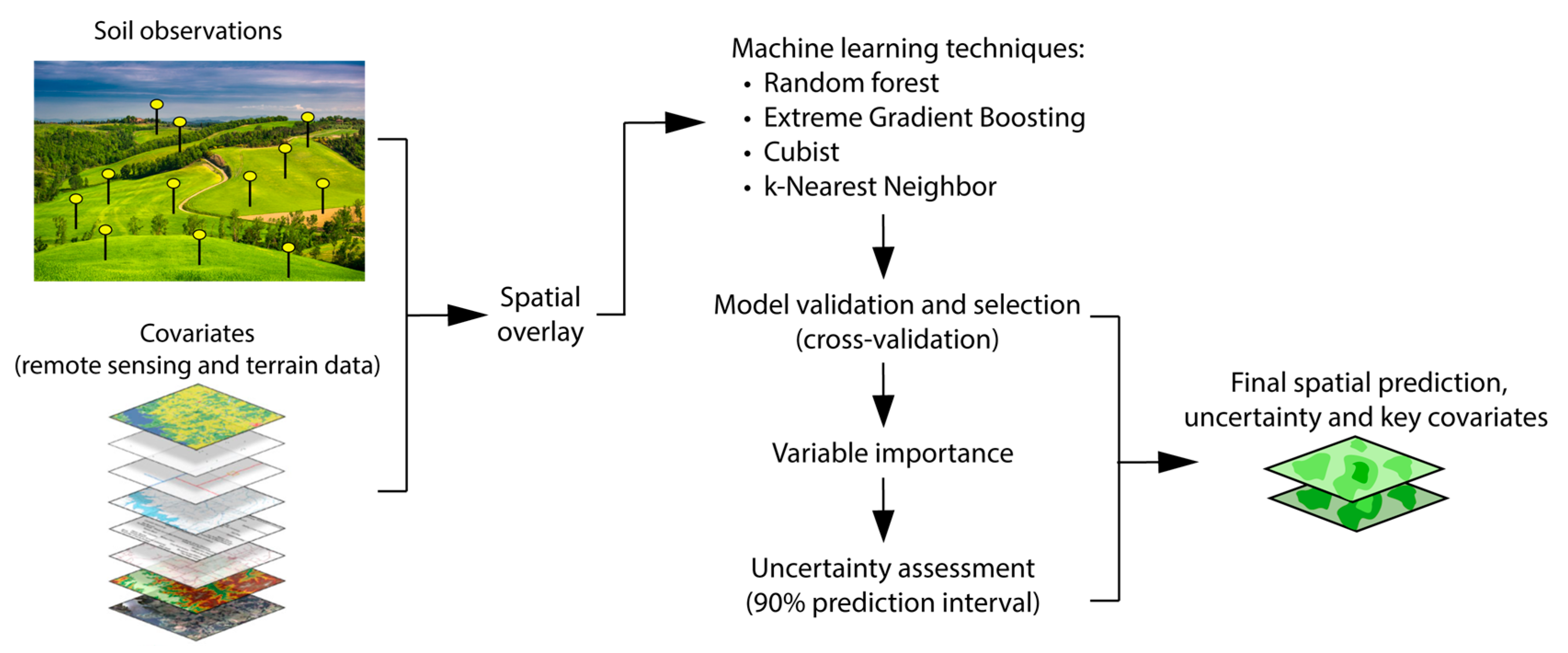
The implementation process of DSM using ML techniques typically involves the following steps. First, datasets with georeferenced soil observations are prepared, where missing values are addressed and variables are normalized (e.g., log- or square-root transformation) (see Section 2.2.). Next, a set of environmental covariates is selected based on expert knowledge and statistical techniques. These covariates can include terrain attributes derived from DEM, spectral indices from RSD, climate variables or any other relevant spatial data. The selection process can be based on prior knowledge, expert judgment or statistical techniques such as correlation analysis or principal component analysis. Then, the procedure of extracting the values of selected covariates in the soil observation sites is carried out. This involves overlaying the covariate layers with the spatial coordinates of the soil points to obtain a set of predictor variables for each observation. After that, a ML method is applied and its accuracy is evaluated using a cross-validation procedure and error metrics. Next, a trained and validated ML model is employed throughout the entire study area to predict the soil properties across the landscape. The covariates selected as inputs generate a continuous or categorical map of the soil properties of interest. The resulting soil maps provide spatially explicit information on soil distribution and variability. In addition, uncertainty is estimated and the most important predictors that contribute to the effectiveness of the model are identified. In this way, the results are effectively communicated to stakeholders, land managers or policymakers, highlighting the implications of the soil mapping outcomes and the associated uncertainties. A flowchart of the soil Hg map production is shown in Figure 2.

3.1. Enviromental Covariates and Processing

We used RSD and topographic attributes as explanatory variables for spatial modeling of the Hg content. One cloud-free Sentinel-2A scene was downloaded from the Copernicus open access hub, covering the study area. Then, we calculated the spectral indices, including vegetation, soil, brightness and other factors (Table A1). DEM (SRTM) with a 30 m resolution was used for deriving the relief attributes. We calculated slope, aspect, Multi-resolution ridge top flatness index (MrRTF) and Multi-resolution Valley Bottom Flatness (MrVBF) maps. Thus, we used the basic Sentinel-2A bands (B02-B12) and derived spectral indices and relief attributes as covariates.
To avoid multicollinearity, we excluded highly correlated covariates using the function findcorrelation in R language. We applied a Spearman correlation approach and removed raster with r > 0.95. A total of 16 covariates were left for further digital mapping. Then, the recursive feature elimination (RFE) algorithm was used to select the most significant auxiliary variables in predicting the Hg content using ML approaches.

3.2. Machine Learning

We used a number of ML methods for the spatial modeling of the Hg content, which are widely known and actively used in DSM [35,36,37,38,39].

3.2.1. Random Forest (RF)

Random Forest is a popular ML algorithm used in DSM to predict soil properties and classes. RF can handle a large number of predictor variables, identify non-linear relationships between variables and account for interactions between variables [40]. RF is stable against overfitting and consists of numerous individual tree models trained from bootstrap samples of the data. The results of all individual trees are aggregated to make a single prediction.

3.2.2. Extreme Gradient Boosting (XGboost)

XGBoost is a popular ML algorithm that has been successfully used in DSM studies. It is a powerful technique that combines multiple decision trees to create a strong predictive model [41]. The XGBoost algorithm works by iteratively improving the performance of a weak learner (a decision tree) by building new trees that correct the errors of the previous ones. During each iteration, the algorithm calculates the gradients and the Hessians of the loss function with respect to the predictions of the previous trees. These values are used to determine the direction and magnitude of the changes to be made to the model’s parameters.

3.2.3. Cubist

Cubist is a decision tree–based model that is particularly suited for handling high-dimensional data and capturing nonlinear relationships between variables. This algorithm works by building a set of decision trees, each of which partitions the input space into regions based on the values of the input variables [42]. The output of each tree is a linear model that predicts the value of the target variable within the corresponding region. The final prediction is obtained by aggregating the predictions of all the trees.

3.2.4. k-Nearest Neighbor (kNN)

kNN is algorithm that can be used for a variety of tasks, including DSM. It is a non-parametric technique used for classification and regression analysis. In this method, the classification of a new data point is determined by identifying the k number of data points in the training set that are closest to it, based on a distance metric [43]. The classification of the new point is then determined by the majority class of the k nearest neighbors.

3.3. Validation and Uncertainty Analysis

This study used a Leave-one-out (LOO) cross-validation method to evaluate the predictive performance of the above ML models. The model performance was measured by the mean absolute error (MAE) and the root mean square error (RMSE). Models with the lowest MAE and RMSE values were deemed the best models.
The spatial uncertainty of predicted Hg values was estimated by computing maps of the lower and upper limits of the 90% prediction intervals. A 90% prediction interval is a range of values that is expected to contain a future observation with a probability of 90%. Thus, we computed the upper (Q95) and lower (Q5) percentiles for each pixel and then estimated uncertainty as the difference between the 95th and the 5th percentiles (i.e., 90% prediction interval).

3.4. Software

Data preprocessing, statistical analysis and digital mapping were performed on R language and environment computing (R Development Core Team).

4. Results

4.1. Mercury Content

Table 1 presents the general statistical results of the Hg concentrations, including minimum, maximum, mean, Standard Deviation (SD), Coefficient of Variation (CV), kurtosis and skewness. The results show that the Hg content varied from 0.005 to 0.58 mg/kg with an average of 0.05 mg/kg. The CV of Hg levels was 123.8%, indicating that the SD was much larger than the mean and that the data had a high degree of variability. A positive kurtosis value of 30.1 indicates that the distribution is heavily-tailed or has outliers, meaning that there are a few observations that are significantly different from the rest of the data. This suggests that the distribution is not normal or symmetric. Figure 3 shows the histogram of log transformed data and the variogram of the Hg content. According to the variogram, the Hg concentrations were characterized by an absence of spatial dependence, i.e., the pure nugget effect.

4.2. Model Performance

Based on the MAE and RMSE error metrics, the results showed that among the applied ML techniques, the RF had the highest performance in predicting the Hg content (0.029 and 0.065 mg/kg, respectively) (Table 2). All the models showed similar metrics, but the XGBoost model showed the lowest values for Hg prediction (MAE = 0.032, RMSE = 0.073 mg/kg).

4.3. Optimal Number and Relative Importance of Environmental Variables

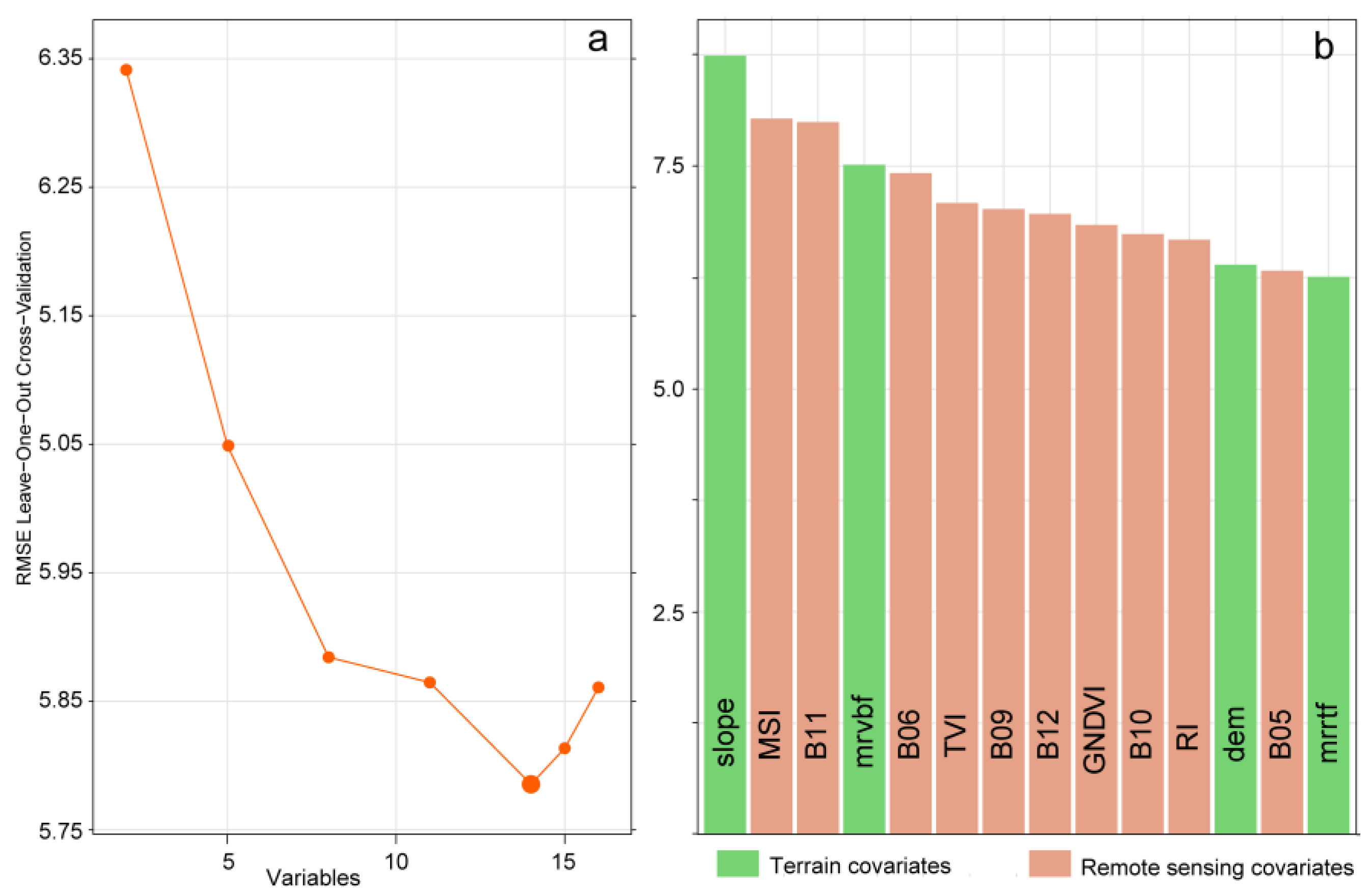
Figure 4 shows the optimal number and relative importance of environmental variables used in the RF prediction of the Hg content. The optimal number of covariates included in the RF predictive model was 14, combining both RSD and terrain attributes. This model included 4 terrain and 10 RSD variables. We found that the slope, spectral index MSI and B11 band were the most effective covariates in predicting the Hg content using the RF model. Their relative importance was 8.7% for the slope, 8% for MSI and 7.9% for B11.

4.4. Generated Digital Map and Uncertainty

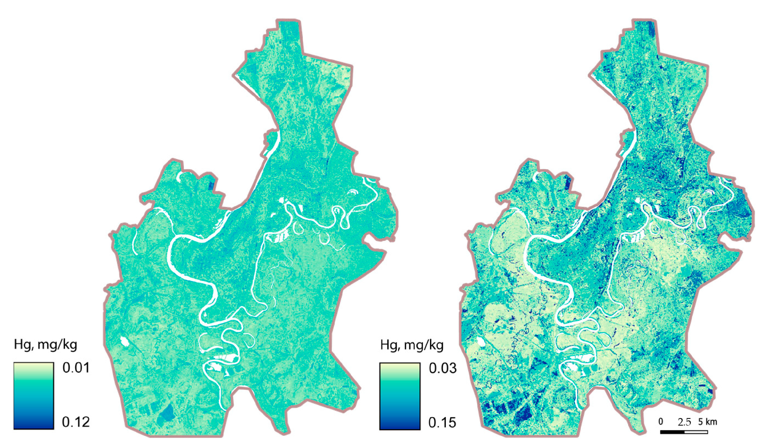
Figure 5 shows the predicted soil Hg concentration and uncertainty maps using the RF model. The predicted Hg values in Ufa ranged from 0.01 to 0.12 mg/kg. We found that the elevated Hg levels were observed mainly on the peninsula and in the northern part, where most of the residential areas with very dense buildings, industrial facilities and factories are located (see Figure 1). At the same time, the predicted highest Hg values were also concentrated in arable plots outside the urban area.
The prediction limit in the 90% prediction interval (PI), which is the difference between the upper and lower limits, ranged between 0.03 and 0.15 mg/kg. According to the produced uncertainty map, the highest uncertainty of Hg values was found on croplands and in urban areas on the peninsula and beyond its borders. The lowest levels were found in open areas with forest vegetation in the city boundaries and around the peninsula. Thus, the map pixels with lower uncertainty values had a narrower range of potential Hg values, and therefore the predicted Hg value is more certain. Conversely, pixels with higher uncertainty values had a wider range of potential Hg values, and therefore the predicted Hg value is less certain.

5. Discussion

5.1. Mercury Content

The Hg concentrations in the soils of Ufa varied widely and were generally comparable with those of other cities. For example, Yang et al. [44] found that the Hg content was 0.026–1.432 mg/kg in a 0–20 cm soil layer in the Changchun urban area (China). In St. Petersburg (Russia), these values ranged from 0.01–2.4 mg/kg at a similar depth [2]. The soils of one of the parks were studied directly in Ufa City, where the Hg content was in the range of 0.019–0.067 mg/kg in the upper soil layer [33].

5.2. Model Performance

The performance of the ML methods was comparable, but the RF method was the most accurate according to the error metrics. In an earlier study, Shi et al. [45] obtained MAE = 0.0082 and RMSE = 0.0112 mg/kg values when modelling Hg concentration using a RF method in Huanghua City (China). The superiority of RF has been demonstrated in many works. For instance, Azizi et al. [14] showed that a RF approach was highly accurate in predicting Ni and Cu contents, while a Cubist model was more accurate in predicting manganese content in western Iran. This justifies the necessity of testing several methods for more accurate spatial prediction of HM, soil properties or classes [37,38,39].
Although in our study the Hg content did not have any spatial correlation, in future studies geostatistical and hybrid methods can improve the accuracy of the spatial predictions. For example, Fu et al. [46] employed a geographically weighted regression approach to spatially map the distribution of soil HM in Daye City, China. Sergeev et al. [47] adopted an artificial neural network plus kriging of the residuals to model the spatial distribution of HM in Novy Urengoy, Russia. Thus, the spatial dependence of HM can be used to improve DSM results.

5.3. Importance of Covariates

Analysis of the importance of auxiliary variables showed that slope map, followed by MSI index and B11 band, was most important to the digital mapping of the Hg content. Thus, RSD and topographic attributes are important covariates together. The importance of topography in HM modelling, including ML methods, has been demonstrated in previous studies [48,49].
The MSI index based on the division of SWIR1 (B11) and NIR bands, as well as the B11 band, were most important for the spatial prediction of the Hg content. Thus, it can be assumed that the wavelengths concentrated around 833 (B8) and 1613 nm (B11) were sensitive to the soil Hg content through the absorption features of auxiliary objects (urban and pristine) in our study. In a previous study, Evangelou et al. [50] found that the best wavelengths for studying soil Hg were 1140–1200 nm using Hyperspectral MAPper data.
HM at low concentrations has no spectral characteristics and its successful spatial modelling is achieved through correlations with soil and plant characteristics [51]. Numerous studies have reported that the Hg content of soils is absorbed by iron and aluminium oxides, clay minerals and organic matter, which in turn have specific absorption features [52,53,54]. Thus, RSD serves as a valuable tool for determining the co-variation between soil characteristics and HM content. For instance, Ballabio et al. [55] estimated the spatial distribution of Hg content in the soils of Europe and revealed the relationship between its content and NDVI, as high NDVI reflects vegetation activity, and its values were most often associated with high soil organic carbon concentrations. Similarly, it was shown that the main variables responsible for the distribution of HM in arid soils were the RSD from January and February, due to climate and vegetation cover in this season [56].

5.4. Uncertainty and Limitations

The range of uncertainty values that we obtained suggests that the uncertainty in our predictions varies widely across our map. We found that the higher uncertainty values of soil Hg were found in arable areas, as well as in urban residential and industrial areas. We suggest that in the case of croplands, the high uncertainty is due to the lack of soil samples from these sites, which have an open soil surface and a unique spectral response. In urban areas, such uncertainty may be attributed to the high spatial variability of soil properties due to anthropogenic influences and the corresponding low accuracy of the prediction. Therefore, the high degree of heterogeneity in urban soils can make it difficult to accurately represent the variability of soil properties and HM contents. Besides soil measurements and positional accuracy, one potential source of uncertainty is the selection and quality of covariates [57]. Thus, we conclude that the digital mapping of the Hg content in urbanized areas using this set of explanatory variables is limited. Pristine landscapes, such as forests and parks, were characterized by less uncertainty. Therefore, the lower uncertainty values may also be associated with the relatively flat relief of the study area and homogeneous spectral reflectance of forests.
Urban soils pose significant challenges to DSM techniques due to their complex and heterogeneous nature, limited data availability and the need to account for anthropogenic influences [31]. Numerous studies have achieved good results in the digital mapping of HM by adding anthropogenic variables. For example, it was previously shown that anthropogenic factors played an important role in lead modeling. In particular, Pb content was mainly influenced by the distance from industrial enterprises and gas stations, as well as by population density [49]. In another study, anthropogenic parameters such as proximity to the road, the image in night light and the distance to environmental hot spots were of high relative importance for modeling Zn, Pb and Cu concentrations [56].

6. Conclusions

Digital mapping of heavy metals (HM) distribution in soils is crucial for identifying areas at risk of contamination and developing effective strategies for managing and mitigating its effects, especially in urban landscapes. In this study, we applied machine learning (ML) techniques such as Random Forest (RF), Extreme Gradient Boosting (XGboost), Cubist and k-Nearest Neighbor (kNN) in combination with remote sensing data (RSD) and relief covariates to map Hg content. The RF method was found to be the most accurate in spatial prediction for Hg content. The study also identified key variables such as slope map, spectral index MSI and Sentinel-2A band B11 for explaining the variability of soil Hg content. Overall, this study provides valuable insights into the potential of ML techniques for identifying areas at risk of Hg contamination, which can inform land-use planning and management strategies to protect human health and the environment. Nevertheless, we conclude that further steps should be taken to improve the spatial prediction of HM in heterogeneous landscapes, such as urban environments:
  • ML approaches in urban environments should be used in combination with other covariates that primarily affect HM concentrations, such as geology and anthropogenic variables. In open pristine landscapes, maps of soil properties (soil organic carbon or pH) that are characterized by a relationship to HM content should be included as explanatory variables.
  • Testing methods that take into account the spatial dependence of soil properties, from simple geostatistical methods (e.g., ordinary kriging, IDW) to hybrid methods such as regression kriging or ML methods plus residuals kriging, should be used.

Author Contributions

Conceptualization, A.S. and R.S.; methodology, A.S., R.S. and A.K.; software, A.S.; investigation, A.K.; data curation, R.S., A.K. and M.Y.; writing—original draft preparation, A.S.; writing—review and editing, R.S. and M.Y.; visualization, A.S.; supervision, A.K.; funding acquisition, R.R. and M.Y. All authors have read and agreed to the published version of the manuscript.

Funding

This research was funded by the Ministry of Science and Higher Education of the Russian Federation № FMRS-2023-0006, FMEN 2022-0012, FMEN 2022-0014.

Data Availability Statement

Data may be requested from the corresponding author for an appropriate reason.

Conflicts of Interest

The authors declare no conflict of interest.

Appendix A

Table A1. Derived remote sensing and topographic attributes used for ML modeling (the basic bands of Sentinel-2A are not specified).
AttributeAcronymEquationReference
Normalized RedRn R R   +   G   +   B [58]
Normalized GreenGn G R   +   G   +   B [58]
Normalized BlueBn B R   +   G   +   B [58]
Normalized Difference Vegetation IndexNDVI NIR R NIR + R [59]
Green Normalized Difference Vegetation IndexGNDVI NIR G NIR + G [60]
Enhanced Vegetation IndexEVI A ( NIR R NIR + C 1 R C 2 B + L )[61]
Colour IndexCI R G R + G [62]
Brightness IndexBI ( R R ) + ( G G ) 2 [63]
Brightness Index 2BI2 ( R R ) + ( G G ) + ( NIR NIR ) 3 [63]
Transformed Vegetation IndexTVI( NIR R NIR + R + 0.5 ) 1 / 2     100 [64]
Soil Adjusted Vegetation IndexSAVI ( NIR R ) ( 1 + L ) NIR R + L [61]
Soil-Adjusted Total Vegetation IndexSATVI SWIR1 R SWIR1 + R + L ( 1 + L )   SWIR2 / 2 [65]
Redness IndexRI R R G G G [62]
Moisture Stress IndexMSI SWIR1 NIR [66]
Land Surface Water IndexLSWI NIR SWIR1 NIR SWIR1 [67]
Green-Red Vegetation IndexGRVI G R G + R [68]
Saturation IndexSI R B R   +   B [69]
ElevationDEM-SRTM
SlopeSlope-SRTM
AspectAs-SRTM
Multi-Resolution Ridge Top FlatnessMrRTF-SRTM
Multi-Resolution Valley Bottom FlatnessMrVBF-SRTM

References

  1. Balali-Mood, M.; Naseri, K.; Tahergorabi, Z.; Khazdair, M.; Sadeghi, M. Toxic Mechanisms of Five Heavy Metals: Mercury, Lead, Chromium, Cadmium, and Arsenic. Front. Pharmacol. 2021, 12, 643972. [Google Scholar] [CrossRef] [PubMed]
  2. Polyakov, V.; Kozlov, A.; Suleymanov, A.; Abakumov, E. Soil Pollution Status of Urban Soils in St. Petersburg City, North-West of Russia. Soil Water Res. 2021, 16, 164–173. [Google Scholar] [CrossRef]
  3. Yang, Q.; Zhang, L.; Wang, H.; Martín, J.D. Bioavailability and Health Risk of Toxic Heavy Metals (As, Hg, Pb and Cd) in Urban Soils: A Monte Carlo Simulation Approach. Environ. Res. 2022, 214, 113772. [Google Scholar] [CrossRef]
  4. Bradl, H.B. (Ed.) Sources and Origins of Heavy Metals. In Interface Science and Technology; Heavy Metals in the Environment: Origin, Interaction and Remediation; Elsevier: Amsterdam, The Netherlands, 2005; Chapter 1; Volume 6, pp. 1–27. [Google Scholar]
  5. Opekunova, M.; Opekunov, A.; Somov, V.; Kukushkin, S.; Papyan, E. Transformation of Metals Migration and Biogeochemical Cycling under the Influence of Copper Mining Production (the Southern Urals). CATENA 2020, 189, 104512. [Google Scholar] [CrossRef]
  6. Suleymanov, R.; Dorogaya, E.; Gareev, A.; Minnegaliev, A.; Gaynanshin, M.; Zaikin, S.; Belan, L.; Tuktarova, I.; Suleymanov, A. Assessment of Chemical Properties, Heavy Metals, and Metalloid Contamination in Floodplain Soils under the Influence of Copper Mining: A Case Study of Sibay, Southern Urals. Ecologies 2022, 3, 530–538. [Google Scholar] [CrossRef]
  7. Malar, S.; Sahi, S.V.; Favas, P.J.C.; Venkatachalam, P. Assessment of Mercury Heavy Metal Toxicity-Induced Physiochemical and Molecular Changes in Sesbania grandiflora L. Int. J. Environ. Sci. Technol. 2015, 12, 3273–3282. [Google Scholar] [CrossRef] [Green Version]
  8. Perugini, M.; Manera, M.; Grotta, L.; Abete, M.C.; Tarasco, R.; Amorena, M. Heavy Metal (Hg, Cr, Cd, and Pb) Contamination in Urban Areas and Wildlife Reserves: Honeybees as Bioindicators. Biol. Trace Elem. Res. 2011, 140, 170–176. [Google Scholar] [CrossRef]
  9. Tangahu, B.V.; Sheikh Abdullah, S.R.; Basri, H.; Idris, M.; Anuar, N.; Mukhlisin, M. A Review on Heavy Metals (As, Pb, and Hg) Uptake by Plants through Phytoremediation. Int. J. Chem. Eng. 2011, 2011, e939161. [Google Scholar] [CrossRef]
  10. Zhao, H.; Wu, Y.; Lan, X.; Yang, Y.; Wu, X.; Du, L. Comprehensive Assessment of Harmful Heavy Metals in Contaminated Soil in Order to Score Pollution Level. Sci. Rep. 2022, 12, 3552. [Google Scholar] [CrossRef]
  11. McBratney, A.B.; Mendonça Santos, M.L.; Minasny, B. On Digital Soil Mapping. Geoderma 2003, 117, 3–52. [Google Scholar] [CrossRef]
  12. Arrouays, D.; McBratney, A.; Bouma, J.; Libohova, Z.; Richer-de-Forges, A.C.; Morgan, C.L.S.; Roudier, P.; Poggio, L.; Mulder, V.L. Impressions of Digital Soil Maps: The Good, the Not so Good, and Making Them Ever Better. Geoderma Reg. 2020, 20, e00255. [Google Scholar] [CrossRef]
  13. Wadoux, A.M.J.-C.; Minasny, B.; McBratney, A.B. Machine Learning for Digital Soil Mapping: Applications, Challenges and Suggested Solutions. Earth-Sci. Rev. 2020, 210, 103359. [Google Scholar] [CrossRef]
  14. Azizi, K.; Ayoubi, S.; Nabiollahi, K.; Garosi, Y.; Gislum, R. Predicting Heavy Metal Contents by Applying Machine Learning Approaches and Environmental Covariates in West of Iran. J. Geochem. Explor. 2022, 233, 106921. [Google Scholar] [CrossRef]
  15. Kirkwood, C.; Cave, M.; Beamish, D.; Grebby, S.; Ferreira, A. A Machine Learning Approach to Geochemical Mapping. J. Geochem. Explor. 2016, 167, 49–61. [Google Scholar] [CrossRef] [Green Version]
  16. Trifi, M.; Gasmi, A.; Carbone, C.; Majzlan, J.; Nasri, N.; Dermech, M.; Charef, A.; Elfil, H. Machine Learning-Based Prediction of Toxic Metals Concentration in an Acid Mine Drainage Environment, Northern Tunisia. Environ. Sci. Pollut. Res. 2022, 29, 87490–87508. [Google Scholar] [CrossRef] [PubMed]
  17. Chen, H.; Chen, C.; Zhang, Z.; Lu, C.; Wang, L.; He, X.; Chu, Y.; Chen, J. Changes of the spatial and temporal characteristics of land-use landscape patterns using multi-temporal Landsat satellite data: A case study of Zhoushan Island, China. Ocean Coast. Manag. 2021, 213, 105842. [Google Scholar] [CrossRef]
  18. Sun, W.; Liu, K.; Ren, G.; Liu, W.; Yang, G.; Meng, X.; Peng, J. A simple and effective spectral-spatial method for mapping large-scale coastal wetlands using China ZY1-02D satellite hyperspectral images. Int. J. Appl. Earth Obs. Geoinf. 2021, 104, 102572. [Google Scholar] [CrossRef]
  19. Florinsky, I.V.; Eilers, R.G.; Manning, G.R.; Fuller, L.G. Prediction of Soil Properties by Digital Terrain Modelling. Environ. Model. Softw. 2002, 17, 295–311. [Google Scholar] [CrossRef]
  20. Wang, F.; Gao, J.; Zha, Y. Hyperspectral Sensing of Heavy Metals in Soil and Vegetation: Feasibility and Challenges. ISPRS J. Photogramm. Remote Sens. 2018, 136, 73–84. [Google Scholar] [CrossRef]
  21. Hou, S.; Zheng, N.; Tang, L.; Ji, X.; Li, Y. Effect of Soil PH and Organic Matter Content on Heavy Metals Availability in Maize (Zea mays L.) Rhizospheric Soil of Non-Ferrous Metals Smelting Area. Environ. Monit. Assess. 2019, 191, 634. [Google Scholar] [CrossRef]
  22. Kooistra, L.; Wehrens, R.; Leuven, R.S.E.W.; Buydens, L.M.C. Possibilities of Visible–near-Infrared Spectroscopy for the Assessment of Soil Contamination in River Floodplains. Anal. Chim. Acta 2001, 446, 97–105. [Google Scholar] [CrossRef]
  23. Dunagan, S.C.; Gilmore, M.S.; Varekamp, J.C. Effects of Mercury on Visible/near-Infrared Reflectance Spectra of Mustard Spinach Plants (Brassica rapa P.). Environ. Pollut. 2007, 148, 301–311. [Google Scholar] [CrossRef] [PubMed]
  24. Zhao, L.; Hu, Y.-M.; Zhou, W.; Liu, Z.-H.; Pan, Y.-C.; Shi, Z.; Wang, L.; Wang, G.-X. Estimation Methods for Soil Mercury Content Using Hyperspectral Remote Sensing. Sustainability 2018, 10, 2474. [Google Scholar] [CrossRef] [Green Version]
  25. Khosravi, V.; Gholizadeh, A.; Saberioon, M. Soil Toxic Elements Determination Using Integration of Sentinel-2 and Landsat-8 Images: Effect of Fusion Techniques on Model Performance. Environ. Pollut. 2022, 310, 119828. [Google Scholar] [CrossRef] [PubMed]
  26. Mirzaei, F.; Abbasi, Y.; Sohrabi, T. Modeling the Distribution of Heavy Metals in Lands Irrigated by Wastewater Using Satellite Images of Sentinel-2. Egypt. J. Remote Sens. Space Sci. 2021, 24, 537–546. [Google Scholar] [CrossRef]
  27. Taghizadeh-Mehrjardi, R.; Fathizad, H.; Ali Hakimzadeh Ardakani, M.; Sodaiezadeh, H.; Kerry, R.; Heung, B.; Scholten, T. Spatio-Temporal Analysis of Heavy Metals in Arid Soils at the Catchment Scale Using Digital Soil Assessment and a Random Forest Model. Remote Sens. 2021, 13, 1698. [Google Scholar] [CrossRef]
  28. Yang, Y.; Cui, Q.; Jia, P.; Liu, J.; Bai, H. Estimating the Heavy Metal Concentrations in Topsoil in the Daxigou Mining Area, China, Using Multispectral Satellite Imagery. Sci. Rep. 2021, 11, 11718. [Google Scholar] [CrossRef] [PubMed]
  29. Ferreira, C.S.S.; Walsh, R.P.D.; Ferreira, A.J.D. Degradation in Urban Areas. Curr. Opin. Environ. Sci. Health 2018, 5, 19–25. [Google Scholar] [CrossRef] [Green Version]
  30. Seifollahi-Aghmiuni, S.; Kalantari, Z.; Egidi, G.; Gaburova, L.; Salvati, L. Urbanisation-Driven Land Degradation and Socioeconomic Challenges in Peri-Urban Areas: Insights from Southern Europe. Ambio 2022, 51, 1446–1458. [Google Scholar] [CrossRef]
  31. Vasenev, V.I.; Stoorvogel, J.J.; Vasenev, I.I.; Valentini, R. How to Map Soil Organic Carbon Stocks in Highly Urbanized Regions? Geoderma 2014, 226, 103–115. [Google Scholar] [CrossRef]
  32. Suleimanov, R.; Abakumov, E.; Suleymanov, A. Soil-Archaeological Study of the Votikeevo Medieval Archeological Site in the Northern Forest-Steppe Zone of the Southern Cis-Ural Region. Eurasian Soil Sci. 2020, 53, 283–293. [Google Scholar] [CrossRef]
  33. Suleymanov, A.; Suleimanov, R.; Abakumov, E.; Nigmatullin, A.; Khamidullin, R. Soil-Ecological Assessment of the M.I. Kalinin Park Ufa City, Russia. In Green Technologies and Infrastructure to Enhance Urban Ecosystem Services: Proceedings of the Smart and Sustainable Cities Conference 2018; Springer Geography; Springer: Berlin/Heidelberg, Germany, 2020; pp. 18–28. ISBN 978-3-319-89796-7. [Google Scholar]
  34. Potapov, A.I.; Vorobyov, V.N.; Karlin, J.H.; Muzalevsky, A.A. Monitoring, control and management of environmental quality. Part 2. Ecological control. In Scientific, Educational and Methodical Reference Manual; Russian State Hydrometeorological University: St. Petersburg, Russia, 2004; p. 290. [Google Scholar]
  35. Hengl, T.; Heuvelink, G.; Kempen, B.; Leenaars, J.G.B.; Walsh, M.; Shepherd, K.; Sila, A.; Macmillan, R.A.; Mendes de Jesus, J.; Tamene, L.; et al. Mapping Soil Properties of Africa at 250 m Resolution: Random Forests Significantly Improve Current Predictions. PLoS ONE 2015, 10, e0125814. [Google Scholar] [CrossRef]
  36. John, K.; Abraham Isong, I.; Michael Kebonye, N.; Okon Ayito, E.; Chapman Agyeman, P.; Marcus Afu, S. Using Machine Learning Algorithms to Estimate Soil Organic Carbon Variability with Environmental Variables and Soil Nutrient Indicators in an Alluvial Soil. Land 2020, 9, 487. [Google Scholar] [CrossRef]
  37. Khaledian, Y.; Miller, B.A. Selecting Appropriate Machine Learning Methods for Digital Soil Mapping. Appl. Math. Model. 2020, 81, 401–418. [Google Scholar] [CrossRef]
  38. Mahmoudzadeh, H.; Matinfar, H.R.; Taghizadeh-Mehrjardi, R.; Kerry, R. Spatial Prediction of Soil Organic Carbon Using Machine Learning Techniques in Western Iran. Geoderma Reg. 2020, 21, e00260. [Google Scholar] [CrossRef]
  39. Suleymanov, A.; Tuktarova, I.; Belan, L.; Suleymanov, R.; Gabbasova, I.; Araslanova, L. Spatial Prediction of Soil Properties Using Random Forest, k-Nearest Neighbors and Cubist Approaches in the Foothills of the Ural Mountains, Russia. Model. Earth Syst. Environ. 2023. [Google Scholar] [CrossRef]
  40. Breiman, L. Random Forests. Mach. Learn. 2001, 45, 5–32. [Google Scholar] [CrossRef] [Green Version]
  41. Friedman, J.H. Stochastic Gradient Boosting. Comput. Stat. Data Anal. 2002, 38, 367–378. [Google Scholar] [CrossRef]
  42. Kuhn, M.; Johnson, K. Applied Predictive Modeling; Springer: New York, NY, USA, 2013. [Google Scholar]
  43. McRoberts, R.E. Estimating Forest Attribute Parameters for Small Areas Using Nearest Neighbors Techniques. For. Ecol. Manag. 2012, 272, 3–12. [Google Scholar] [CrossRef]
  44. Yang, Z.; Lu, W.; Long, Y.; Bao, X.; Yang, Q. Assessment of Heavy Metals Contamination in Urban Topsoil from Changchun City, China. J. Geochem. Explor. 2011, 108, 27–38. [Google Scholar] [CrossRef]
  45. Shi, S.; Hou, M.; Gu, Z.; Jiang, C.; Zhang, W.; Hou, M.; Li, C.; Xi, Z. Estimation of Heavy Metal Content in Soil Based on Machine Learning Models. Land 2022, 11, 1037. [Google Scholar] [CrossRef]
  46. Fu, P.; Yang, Y.; Zou, Y. Prediction of Soil Heavy Metal Distribution Using Geographically Weighted Regression Kriging. Bull Environ. Contam. Toxicol. 2022, 108, 344–350. [Google Scholar] [CrossRef]
  47. Sergeev, A.P.; Buevich, A.G.; Baglaeva, E.M.; Shichkin, A.V. Combining Spatial Autocorrelation with Machine Learning Increases Prediction Accuracy of Soil Heavy Metals. CATENA 2019, 174, 425–435. [Google Scholar] [CrossRef]
  48. Shi, T.; Hu, X.; Guo, L.; Su, F.; Tu, W.; Hu, Z.; Liu, H.; Yang, C.; Wang, J.; Zhang, J.; et al. Digital Mapping of Zinc in Urban Topsoil Using Multisource Geospatial Data and Random Forest. Sci. Total Environ. 2021, 792, 148455. [Google Scholar] [CrossRef] [PubMed]
  49. Wu, Z.; Chen, Y.; Yang, Z.; Liu, Y.; Zhu, Y.; Tong, Z.; An, R. Spatial Distribution of Lead Concentration in Peri-Urban Soil: Threshold and Interaction Effects of Environmental Variables. Geoderma 2023, 429, 116193. [Google Scholar] [CrossRef]
  50. Evangelou, M.W.H.; Ebel, M.; Schaeffer, A. Chelate Assisted Phytoextraction of Heavy Metals from Soil. Effect, Mechanism, Toxicity, and Fate of Chelating Agents. Chemosphere 2007, 68, 989–1003. [Google Scholar] [CrossRef] [PubMed]
  51. Wu, Y.Z.; Chen, J.; Ji, J.F.; Tian, Q.J.; Wu, X.M. Feasibility of Reflectance Spectroscopy for the Assessment of Soil Mercury Contamination. Environ. Sci. Technol. 2005, 39, 873–878. [Google Scholar] [CrossRef] [PubMed]
  52. Kemper, T.; Sommer, S. Estimate of Heavy Metal Contamination in Soils after a Mining Accident Using Reflectance Spectroscopy. Environ. Sci. Technol. 2002, 36, 2742–2747. [Google Scholar] [CrossRef]
  53. Skyllberg, U.; Bloom, P.R.; Qian, J.; Lin, C.-M.; Bleam, W.F. Complexation of Mercury(II) in Soil Organic Matter: EXAFS Evidence for Linear Two-Coordination with Reduced Sulfur Groups. Environ. Sci. Technol. 2006, 40, 4174–4180. [Google Scholar] [CrossRef] [PubMed]
  54. Yin, Y.; Allen, H.E.; Li, Y.; Huang, C.P.; Sanders, P.F. Adsorption of Mercury(II) by Soil: Effects of PH, Chloride, and Organic Matter. J. Environ. Qual. 1996, 25, 837–844. [Google Scholar] [CrossRef]
  55. Ballabio, C.; Jiskra, M.; Osterwalder, S.; Borrelli, P.; Montanarella, L.; Panagos, P. A Spatial Assessment of Mercury Content in the European Union Topsoil. Sci. Total Environ. 2021, 769, 144755. [Google Scholar] [CrossRef]
  56. Peng, Y.; Kheir, R.B.; Adhikari, K.; Malinowski, R.; Greve, M.B.; Knadel, M.; Greve, M.H. Digital Mapping of Toxic Metals in Qatari Soils Using Remote Sensing and Ancillary Data. Remote Sens. 2016, 8, 1003. [Google Scholar] [CrossRef] [Green Version]
  57. Heuvelink, G. Uncertainty Quantification of GlobalSoilMap Products. GlobalSoilMap: Basis of the Global Spatial Soil Information System. In Proceedings of the 1st GlobalSoilMap Conference, Orléans, France, 7–9 October 2014; pp. 335–340. [Google Scholar] [CrossRef]
  58. Kawashima, S.; Nakatani, M. An Algorithm for Estimating Chlorophyll Content in Leaves Using a Video Camera. Ann. Bot. 1998, 81, 49–54. [Google Scholar] [CrossRef] [Green Version]
  59. Rouse, J.W.; Haas, R.H.; Schell, J.A.; Deering, D.W. Monitoring Vegetation Systems in the Great Plains with ERTS. NASA Spec. Publ. 1974, 351, 309. [Google Scholar]
  60. Gitelson, A.A.; Kaufman, Y.J.; Merzlyak, M.N. Use of a Green Channel in Remote Sensing of Global Vegetation from EOS-MODIS. Remote Sens. Environ. 1996, 58, 289–298. [Google Scholar] [CrossRef]
  61. Huete, A.; Didan, K.; Miura, T.; Rodriguez, E.P.; Gao, X.; Ferreira, L.G. Overview of the Radiometric and Biophysical Performance of the MODIS Vegetation Indices. Remote Sens. Environ. 2002, 83, 195–213. [Google Scholar] [CrossRef]
  62. Pouget, M.; Madeira, J.; Le Floch, E.; Kamal, S. Caracteristiques spectrales des surfaces sableuses de la region cotiere Nord-Ouest de I’Egypte: Application aux donnees satellitaires SPOT. In 2eme JoumCes de T&detection: Caracterisation et Suivi des Milieux Terrestres en Regions Arides et Tropicales, Proceedings of the ORSTOM, Collection Colloques et Seminaires, Paris, France, 4–6 December 1990; UNESCO: Paris, France, 1990. [Google Scholar]
  63. Escadafal, R. Remote Sensing of Arid Soil Surface Color with Landsat Thematic Mapper. Adv. Space Res. 1989, 9, 159–163. [Google Scholar] [CrossRef]
  64. Nellis, M.D.; Briggs, J.M. Transformed Vegetation Index for Measuring Spatial Variation in Drought Impacted Biomass on Konza Prairie, Kansas. Trans. Kans. Acad. Sci. 1992, 95, 93–99. [Google Scholar] [CrossRef]
  65. Marsett, R.C.; Qi, J.; Heilman, P.; Biedenbender, S.H.; Watson, M.C.; Amer, S.; Weltz, M.; Goodrich, D.; Marsett, R. Remote sensing for grassland management in the arid southwest. Rangel. Ecol. Manag. 2006, 59, 530–540. [Google Scholar] [CrossRef]
  66. Rock, B.N.; Vogelmann, J.E.; Williams, D.L. Field and Airborne Spectral Characterization of Suspected Damage in Red Spruce (Picea Rubens) from Vermont; NASA: Washington, DC, USA, 1985.
  67. Xiao, X.; Zhang, Q.; Braswell, B.; Urbanski, S.; Boles, S.; Wofsy, S.; Moore, B.; Ojima, D. Modeling Gross Primary Production of Temperate Deciduous Broadleaf Forest Using Satellite Images and Climate Data. Remote Sens. Environ. 2004, 91, 256–270. [Google Scholar] [CrossRef]
  68. Tucker, C.J. Red and Photographic Infrared Linear Combinations for Monitoring Vegetation. Remote Sens. Environ. 1979, 8, 127–150. [Google Scholar] [CrossRef] [Green Version]
  69. Levin, N.; Ben-Dor, E.; Singer, A. A Digital Camera as a Tool to Measure Color Indices and Related Properties of Sandy Soils in Semi-Arid Environments. Int. J. Remote Sens. 2005, 26, 5475–5492. [Google Scholar] [CrossRef]
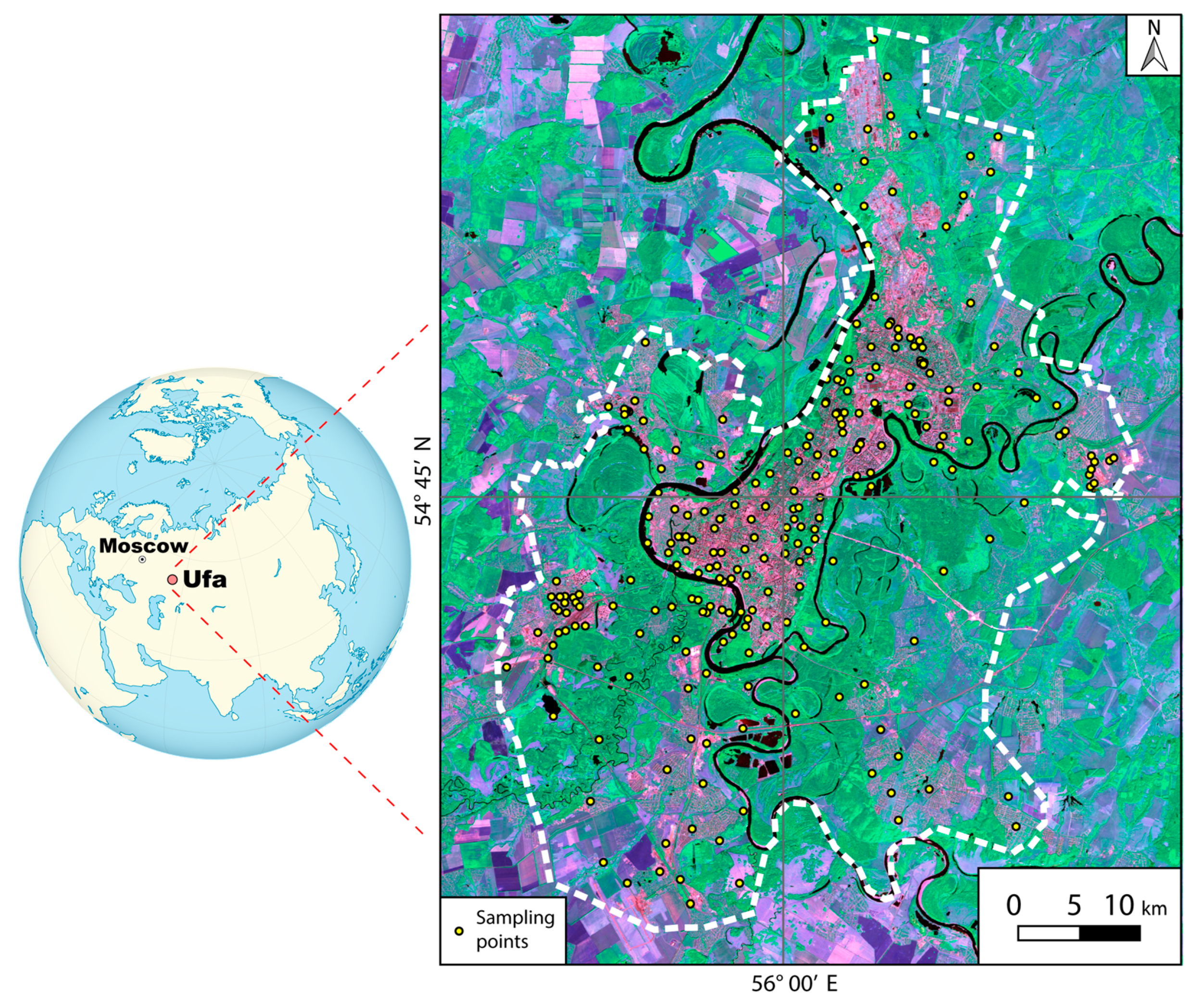
Figure 1. Location of sample sites (yellow dots) in Ufa and adjacent areas. The right figure shows a remote sensing imagery composite (RED-NIR-SWIR), highlighting anthropogenic objects (buildings, roads, arable lands). The white border shows the frame for mapping.
Remotesensing 15 03158 g001
Figure 2. Flowchart of the methodology employed in digital soil mapping of the Hg content.
Remotesensing 15 03158 g002
Figure 3. Histogram of log transformed Hg values and variogram of the Hg content.
Remotesensing 15 03158 g003
Figure 4. The RMSE values for different numbers of variables included in the RF approach as determined by RFE (a) and relative importance of environmental covariates (%) for the Hg content using the RF model (b).
Remotesensing 15 03158 g004
Figure 5. Spatial distribution of the predicted soil Hg values based on the RF model (left) and prediction limit in 90% predicted interval (i.e., difference between upper and lower limits) (right).
Remotesensing 15 03158 g005
Table 1. Statistical parameters of Hg content, mg/kg.
ParameterMinMaxMeanSD 1CV 2KurtosisSkewness
Hg0.0050.580.050.06123.830.14.9
1 Standard variation; 2 Coefficient of variation.
Table 2. LOO cross-validation results of the Hg prediction performance for the ML models.
ML ApproachMAE, mg/kg RMSE, mg/kg
RF0.0290.065
XGBoost0.0320.073
Cubist0.0310.066
kNN0.0310.067
Disclaimer/Publisher’s Note: The statements, opinions and data contained in all publications are solely those of the individual author(s) and contributor(s) and not of MDPI and/or the editor(s). MDPI and/or the editor(s) disclaim responsibility for any injury to people or property resulting from any ideas, methods, instructions or products referred to in the content.