Article

A Prediction Method of Ionospheric hmF2 Based on Machine Learning

1
School of Microelectronics, Tianjin University, Tianjin 300072, China
2
Qingdao Institute for Ocean Technology, Tianjin University, Qingdao 266200, China
3
Shandong Engineering Technology Research Center of Ocean Information Awareness and Transmission, Qingdao 266200, China
*
Author to whom correspondence should be addressed.
These authors contributed equally to this work.
Remote Sens. 2023, 15(12), 3154; https://doi.org/10.3390/rs15123154
Submission received: 17 April 2023 / Revised: 26 May 2023 / Accepted: 12 June 2023 / Published: 16 June 2023

Abstract

:
The ionospheric F2 layer is the essential layer in the propagation of high-frequency radio waves, and the peak electron density height of the ionospheric F2 layer (hmF2) is one of the important parameters. To improve the predicted accuracy of hmF2 for further improving the ability of HF skywave propagation prediction and communication frequency selection, we present an interpretable long-term prediction model of hmF2 using the statistical machine learning (SML) method. Taking Moscow station as an example, this method has been tested using the ionospheric observation data from August 2011 to October 2016. Only by inputting sunspot number, month, and universal time into the proposed model can the predicted value of hmF2 be obtained for the corresponding time. Finally, we compare the predicted results of the proposed model with those of the International Reference Ionospheric (IRI) model to verify its stability and reliability. The result shows that, compared with the IRI model, the predicted average statistical RMSE decreased by 5.20 km, and RRMSE decreased by 1.78%. This method is expected to provide ionospheric parameter prediction accuracy on a global scale.

1. Introduction

The ionosphere is the atmosphere between 60 km and 1000 km above the Earth’s surface. Due to its electrical and ionized structure, and its complex temporal and spatial variability, it is of significant importance for its high frequency (HF) [1]. It influences sky waves, challenging radio propagation and wireless communication [2]. hmF2 is an important parameter of the F2 layer in the ionosphere, which serves as the basis for predicting the usable frequency [3] by reflecting the ionosphere [4]. Namely, usable frequency and propagation loss [5] are a function of hmF2, which indicates the height characteristics and changes of the ionospheric F2 layer [6]. Therefore, a reliable modeling method of hmF2 will help in propagation prediction, frequency selection, and spectrum management for HF communication systems [7]. Moreover, estimating and predicting the characteristics of hmF2 is vital for identifying adverse space weather [8] and hmF2 is a major aeronautical parameter involved in aeronautical [9] and ionospheric electrodynamic [10] studies. In general, the hmF2 can be observed at the sounding station using ionospheric sounders [11]. Without sounding stations, hmF2 can be predicted based on the ionospheric models that provide helpful empirical values for educators, engineers, and scientists.
As an internationally recognized standard, the International Reference Ionosphere (IRI) provides ionospheric parameters [12] and is often used as a benchmark to evaluate the performance of new ionospheric prediction models. Similar to critical frequency and the propagation factor, the modeling methods and models for predicting hmF2 are continuously developing. In order to improve the prediction performance of the ionospheric model, many new methods have constantly been introduced by experts at home and abroad.
For example, based on the empirical orthogonal function, Zhang et al. [13,14] and Yu et al. [15] constructed a global and Chinese ionospheric hmF2 prediction model, respectively, and the results were superior to the IRI model. Themens [16] proposed an ionospheric empirical model of the Canadian high Arctic. Compared with the IRI model, the prediction error of hmF2 of this model was reduced by 3~9 km. Sai et al. established a two-dimensional ionospheric model based on the artificial neural network (ANN) [17] and improved it [18], which can more accurately predict the detailed changes of hmF2 compared with the IRI model. Li et al. [19] established a global ionospheric model based on the improved ANN technology based on the genetic algorithm, which has better temporal and spatial characteristics of the global or regional ionosphere.
To further improve the hmF2 prediction accuracy, we propose an explicable long-term method of hmF2 based on the statistical machine learning (SML) method and the correlation between hmF2 and the solar activity index. The structure is arranged as follows: firstly, the paper elaborates on the SML method, briefly introduces the data required for modeling, and establishes a long-term prediction model for hmF2 based on this data; next, the model prediction results are analyzed, followed by a discussion of the model and a conclusion of the entire paper.

2. Materials and Methods

2.1. Method

Machine learning is an interdisciplinary field that uses probabilistic models to analyze and predict data based on provided data [20]. The idea behind machine learning’s data processing is simple to understand, and the process is straightforward. Unlike the black-box algorithm, the model parameters determined using SML methods have explainable and transparent meanings [21]. For example, SML algorithms can be used to solve specific functional analytic expressions, which deep learning algorithms such as artificial neural networks cannot do [22]. Therefore, statistical machine learning is widely used to model ionospheric parameters. Using SML to reconstruct the ionospheric parameter hmF2 model, it is indispensable to determine the algorithm, strategy, and model with hmF2 data as the core and solve four problems in the process of machine learning:
(1) What data are needed? In machine learning, data are central. The paper is carried out using the data of the median value (the median of each month measured by the hour) calculated from the ionospheric hmF2 observation data of the Moscow station;
(2) How is the model chosen? The selection model finds the mapping relationship between input and output variables. The model should be based on analyzing input and output variables’ characteristics. Ionospheric parameters are affected by solar activities, and there are seasonal, semi-annual, annual, and more subtle changes [23]. Therefore, to establish the hmF2 long-term prediction model, it is necessary to find the mapping relationship between hmF2 and solar activity index and time;
(3) How is the model determined? The model needs to be determined based on the relationship between the independent and target-dependent variables. Here, the relationship between hmF2 and solar activity index and time is determined by regression analysis under the least square;
(4) How is the model evaluated? The discrepancy between the sample’s real output and the learner’s actual predicted output is called an “error”. “Training error” or “empirical error” is the learner’s error on the training set. “Generalization error” refers to the learner’s error on the new sample. Generally, it is desirable to obtain a model with low generalization error. Therefore, the hmF2 data are divided into three parts: training data, verification data, and test data, using training data to train the model and validation data to select and adjust the model. Test data are used to represent the generalization ability of the model [24]. Because of the ionosphere’s prominent time-varying characteristics, this paper uses the relative root mean square error (RRMSE) as the general evaluation standard to evaluate the model.
In brief, this paper uses the RRMSE analysis strategy as the model selection and evaluation criteria to establish the long-term prediction model of hmF2 according to the correlation between the Moscow station’s hmF2 median value data and solar activity and time. Finally, the validity and reliability of the prediction model are verified by the observation data and IRI model. According to the learning process of SML, the following is the process of data acquisition, model training, validation, and testing.
Figure 1 shows the hmF2 modeling process according to SML:
(1) The hmF2 are closely related to solar activity, and there are seasonal, semi-annual, and annual variations. According to the above characteristics, this paper determines the training model set.
(2) The solar activity index, including the solar radio wave flux with a wavelength of 10.7 cm, the number of sunspots, and the strongest single line in the ultraviolet band are selected. The highest power index of solar activity parameters and the highest harmonic number in the trigonometric function is also selected.
(3) Data from August 2011 to December 2015 are used to train, and data from February, March, May, June, August, and September 2016 are used to validate.
(4) The relative root mean square error calculated and recording between the verified and actual data are calculated.
(5) Whether all the highest harmonic numbers in the trigonometric function are traversed is checked. If the traversal is completed, step b is entered; otherwise, the remaining highest harmonic number for model training is selected; Whether all the highest power index of solar activity parameters are traversed is checked. If the traversal is completed, step c is entered; otherwise, the remaining highest power index for model training is selected. Whether the index of solar activity has been traversed is judged. If so, the next step is entered; otherwise, the remaining solar activity indices for training are selected.
(6) The prediction model according to RRMSE is determined.
(7) A modeling test is undertaken. According to the division of seasons, the data of January, April, July, and October 2016 are respectively used for testing and compared with the IRI-2016 model. If the model performance is worse than the IRI model, the data characteristics need to be re-analyzed to determine the model set; if the model performance is better than the IRI model, it can be used for engineering prediction.

2.2. Data

Following the modeling technique route and flow identified in the previous section, this section specifies the data required for hmF2 parameter modeling.

2.2.1. Ionospheric hmF2

hmF2 data from the Moscow station (55.9°N, 37.7°E) are selected to train and learn the proposed model and parameters, which can be obtained from http://www.wdcb.ru (accessed on 1 January 2023) and were measured by an instrument known as the ionosonde. The collected data were averaged by month and hour to obtain the corresponding median value, which is the target variable modeled in this paper and referred to as hmF2 monthly median value data. Figure 2 shows the hmF2 monthly value data of the collected station, which was completed from August 2011 to October 2016 and used in this study to train and validate the proposed model.

2.2.2. Solar Activity Index

People usually use the solar activity index to represent the intensity of solar activity. The most commonly used solar activity index includes: (1) F10.7 [25], the solar radio wave flux with a wavelength of 10.7 cm affected by the upper atmosphere and chromospheric corona [26], denoted simply as F; (2) R [27], the number of sunspots affected by the lower chromosphere and the photosphere; (3) Lyman-α [28], the strongest single line in the ultraviolet band, abbreviated as A. The three solar activity indices are available from the corresponding forecast websites.
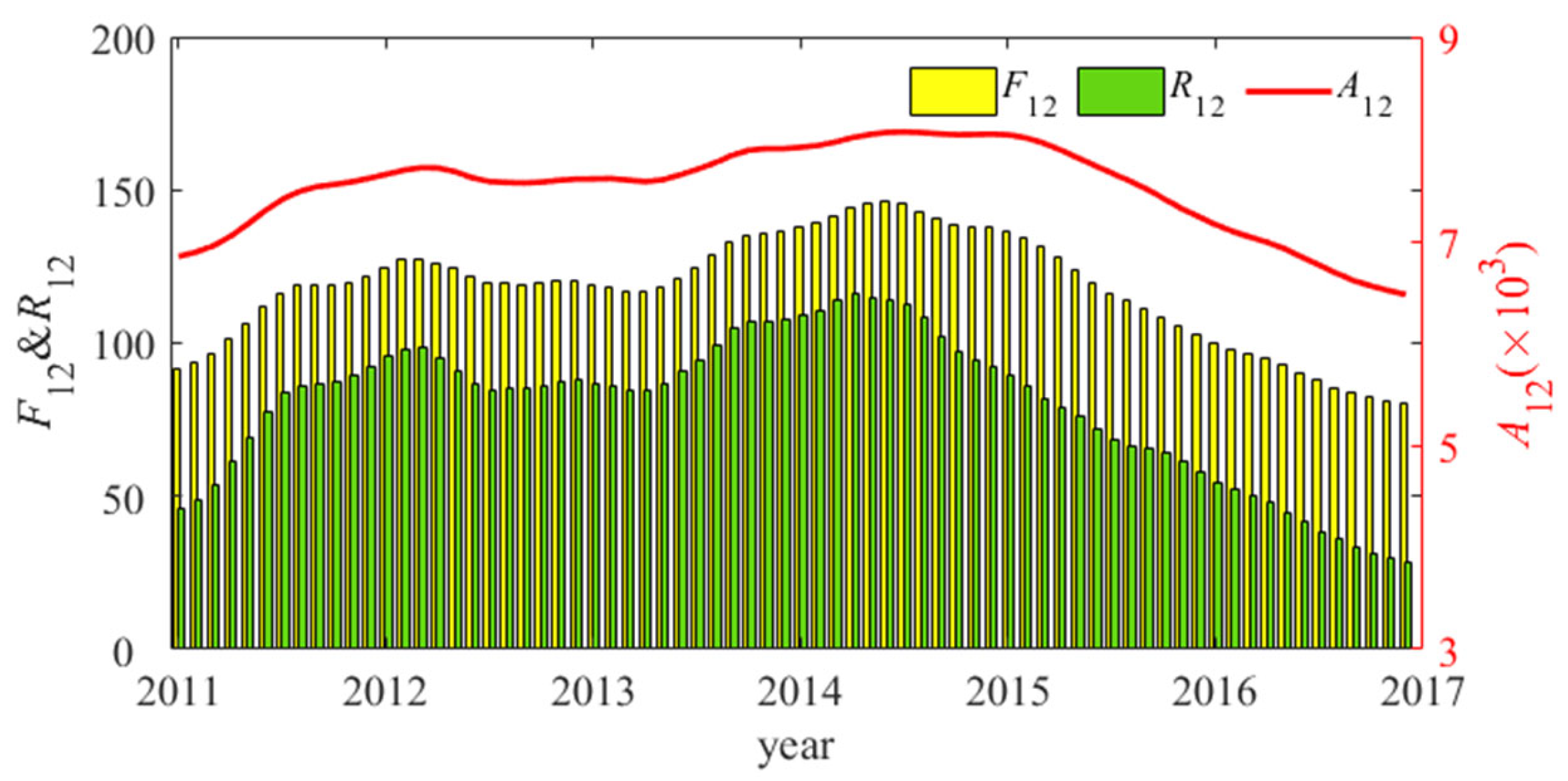
(1) The outer chromosphere and part of the inner corona of the sun’s atmosphere emit F10.7. Flux (sfu) is the unit of F10.7, 1 sfu =10−22 Wm−2Hz−1 [29]. As a common index of solar activity, F10.7 is closely related to the intensity of solar activity [30]. It is mainly determined by sunspot number groups on the solar surface and can describe the intensity of solar activity [31]. It is widely used in ionospheric parameter prediction models. For example, F10.7 is used as the input parameter of the model to fit the ionospheric parameter hmF2 [13,14]. The twelve-monthly smoothed value of F10.7 is used here, denoted as F12.
(2) The sunspot number is a swirling airflow caused by the solid solar magnetic field activity located in the solar sphere [32]. The sunspot number is often used to measure the level of solar activity. Changes in the ionosphere are subject to solar activity, and so the sunspot number is used to describe changes in ionospheric parameters and to study prediction models of ionospheric parameters [31]. Li et al. introduced sunspot numbers into the model when predicting ionospheric hmF2 [19]. The twelve-monthly smoothed value of R is used here, denoted as R12.
(3) The Lyman-α line is the hydrogen line in the Lyman series and represents the most vital single line in the outer band. Electron transitions produce it within hydrogen atoms when atomic electrons transition from the first excited state to the ground state. Lyman-α is released by hydrogen produced in large quantities in the universe [33] and also participate in the modeling of ionospheric parameters as an input parameter [34]. Here, the twelve-monthly smoothed value of Lyman-α is used, denoted as A12.
The twelve-monthly smoothed value is calculated by the following formula:
S 12 = 1 12 i = n 5 n + 5 S ¯ i + 1 2 ( S ¯ n 6 + S ¯ n + 6 )
where S represents the index of solar activity, S ¯ represents the solar activity index’s monthly mean value, and n represents the month.
Figure 3 shows the changes in F12, R12, and A12 over time. The three solar activity indices tend to be the same year by year, but the details are still different.

3. Results

3.1. Model Determination

There is a correlation between ionospheric parameters and the solar activity index, and there are annual, semi-annual, seasonal, and more subtle variations [23] Therefore, for the given local time and geographical coordinates, the Formula (2) shows the general formula for defining the harmonic mapping between the solar cycle variation parameters, year, season, and month, and hmF2:
hmF 2 ( p , m ) = k = 0 K j = 0 J γ k , j p j cos ( 2 π k m / 12 ) + β k , j p j sin ( 2 π k m / 12 )
where p represents F12, R12, A12 and m represents the integer of the month. The harmonic number k describes the variation characteristics of annual, semi-annual, seasonal, and monthly cycles. k = 1, 2, 3, and 4, respectively, represent one year, half a year, a quarter, and one month. Considering that the increase in the K value does not bring a significant increase in calculation accuracy [35], K = 1 and 2 are chosen here. The value of j is directly related to the solar activity index. J = 1 and 2 are selected here. Given the solar activity index and the values of K and J, the hyperparameters in the model can be statistically obtained by regression analysis under the least square method. The final determination of the model requires the consideration of RRMSE. The specific solving process is as follows:
C C T γ 0 , 0 γ 0 , 1 β K , J 1 β K , J = C hmF 2 1 hmF 2 2 hmF 2 O 1 hmF 2 O
where O is the number of hmF2 obtained statistically, and
C = 1 1 1 ( p ) 1 ( p ) 2 ( p ) O ( p ) 1 J 1 sin 2 π K m 12 ( p ) 2 J 1 sin 2 π K m 12 ( p ) O J 1 sin 2 π K m 12 ( p ) 1 J sin 2 π K m 12 ( p ) 2 J sin 2 π K m 12 ( p ) O J sin 2 π K m 12
In the given model set, the data from August 2011 to December 2015 are used for training to obtain the hyperparameters in the model. Then, the data from February, March, May, June, August, and September 2016 are used to verify the trained model. The RRMSE between the verified and observations is calculated, and RRMSE is taken as the evaluation strategy of the model. Formula (5) is the calculation formula of RRMSE:
RRMSE = 1 N i = 1 N ( hmF 2 i hmF 2 i hmF 2 i ) 2
where hmF 2 i is the calculated value of the model, hmF 2 i is the measured statistical value, and N is the total data count.
We calculated the RRMSE value obtained by verification calculation of all training models in the model set. The result shows that: (1) the increase of orders J and K does not improve the model’s predictive performance, but improve the calculation of the algorithm; (2) RRMSE is minimum when R is selected as the index of solar activity to participate in the modeling. The minimum RMSE of using F, R, and A is 4.52%, 4.27%, and 4.67% with J = 1 and K = 1. This is different from the model of ionospheric foF2 [1] and other parameters [35].

3.2. Results Analysis

Based on the training results, the values of p, J, and K were selected as R, 1, and 1, respectively, and then plugged into Equation (2). This led to the derivation of the prediction model for hmF2 at the Moscow station, which is represented by Equation (6):
h ^ mF 2 R , m = k = 0 1 j = 0 1 γ k , j R j cos 2 π k m 12 + β k , j R j sin 2 π k m 12 = γ 0 , 0 + γ 0 , 1 R + γ 1 , 0 + γ 1 , 1 R cos 2 π m 12 + β 1 , 0 + β 1 , 1 R sin 2 π m 12 = γ 0 , 0 + γ 1 , 0 cos 2 π m 12 + β 1 , 0 sin 2 π m 12 + γ 0 , 1 + γ 1 , 1 cos 2 π m 12 + β 1 , 1 sin 2 π m 12 R ,
The exact value of the hyperparameter in the model can be obtained by substituting the training data into Equation (6) and using the least square method to fit it. The result is shown in Figure 4, where the rows represent the world from UT = 0 to UT = 23, the columns represent the names of the hyperparameters, and the colors represent the values of the hyperparameters.
As can be seen from Figure 4, the change of the hyperparameter changes obviously with time, and the γ 0 , 0 is the maximum. With the increase in the order, the value contribution of the hyperparameter decreases.
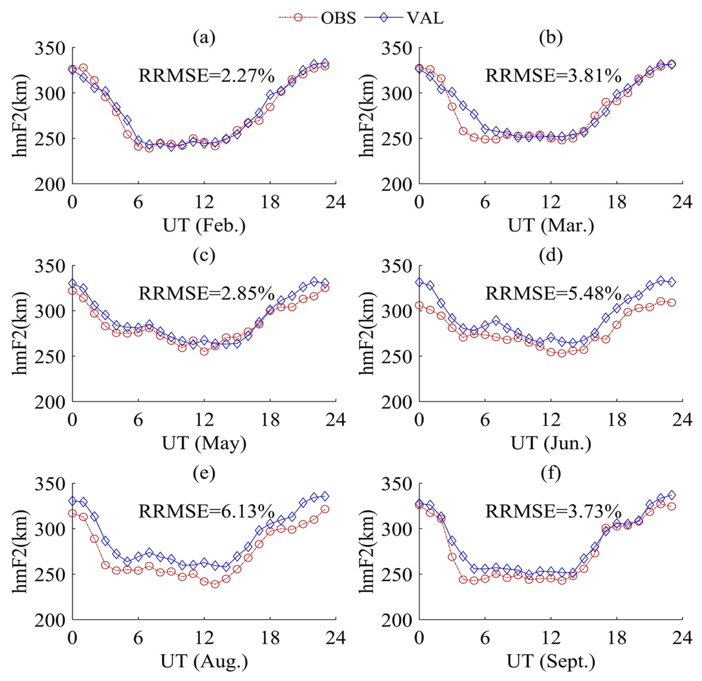
Based on the above conditions, it is only necessary to provide the sunspot number, month, and universal time corresponding to the time in the model to obtain the predicted value of hmF2. In Figure 5, we present the RRMSE between the observations and the predicted values obtained by using the verification dataset, where OBS is the observed value and VAL is the model validation value.
As shown in Figure 5, the model’s predicted ability varies for different months. The RRMSE is less than 3% for February and May, while the predicted ability is relatively poor for July and August, with RRMSE greater than 5%. Furthermore, the predicted values are generally higher than the observations.

4. Discussions

To test the generalization ability of the model, we compared the proposed model (denoted as PRO) with the IRI model [36]. The test data used are hmF2 of January (winter), April (spring), July (summer), and October (autumn) of 2016.
Figure 6 compares the observations, predicted values of the IRI model and PRO model.
Overall, the hmF2 exhibit a trend of being low during the day and high at night. In January and October, the hmF2 values are relatively stable, while, in April and July, they fluctuate to some extent at UT = 7 and UT = 15, respectively. The predicted values of the IRI and PRO models for January and October are relatively close to the observations, but the IRI model tends to overestimate the hmF2 values. However, the IRI and PRO models show significant prediction errors compared with the observations in April and July. Specifically, the predicted values of the IRI model are lower than the observations around UT = 6, while the PRO model’s predictions are higher than the observations.
To further evaluate the model’s predicted ability and accuracy, RRMSE (Equation (7)) and RRMSE (Equation (4)) is calculated to intuitively analyze the difference between hmF2 predicted by the IRI model and the PRO model and the observed value.
Formula (7) is the calculation formula of RMSE:
RMSE = 1 N i = 1 N ( hmF 2 i hmF 2 i ) 2
where hmF 2 i is the calculated value of the model, hmF 2 i is the measured statistical value, and N is the total data count.
Figure 7 shows the RMSE and RRMSE results of the IRI and PRO models. To conduct a more refined analysis of the results, we also calculated the error of the prediction results in different months. The results are shown as follows:
(1) For all the predictions, the RMSE of the IRI model is 17.02 km, and that of the PRO model is 11.82 km. Compared with the IRI model, the RMSE of the PRO model is 5.20 km smaller, proving that the PRO model’s stability is better than that of the IRI model.
(2) Specific to each month, the RMSE of the PRO model is smaller than that of the IRI model. In January and October, the RMSE of the PRO model was much smaller than that of the IRI model. In April, the RMSE of the PRO model was only slightly lower than that of the IRI model. Compared with other months, the RMSE of both models was relatively large in July.
(3) The total RRMSE of the IRI model is 6.01%, and that of the PRO model is 4.23%. Compared with the IRI model, the RRMSE of the PRO model is 1.78% smaller, proving that the PRO model’s prediction accuracy is better than that of the IRI model.
(4) In each month, except April, the RRMSE of the PRO model is smaller than that of the IRI model in other months. In January and October, the RRMSE of the PRO model decreased most significantly compared with the IRI model. Compared with other months, the RRMSE of both models was relatively large in July.
Generally speaking, the PRO model is superior to the IRI model in both stability and accuracy of hmF2 prediction at the Moscow station. In other words, the PRO model improves the predicted accuracy at the Moscow station. The following are our reflections on the results and prospects for the future:
(1) During January and October, the hmF2 of observation showed relatively stable changes, and the PRO model demonstrated a noticeably better predicted ability for the hmF2 data than the IRI model. However, in April and July, the hmF2 exhibited significant fluctuations, causing a decrease in the predicted ability of both models. This suggests that there is room for improvement room in both models to learn the finer details;
(2) The PRO model utilized J = 1 and K = 1 as its model parameters, which differs from other research findings. This phenomenon could be attributed to the size of the collected data, which warrants further exploration. This choice could also result in a weaker generalization ability of the model towards hmF2 details, which also requires further investigation;
(3) Due to data collection limitations, the model could only verify hmF2 data collected from the Moscow station. Future efforts will aim to verify hmF2 data from stations in different latitude regions;
(4) In the future, his model can also be compared with other models such as ANN and LSTM.

5. Conclusions

Based on the SML method, this paper proposed an interpretable long-term prediction model for the ionospheric hmF2 median value of the Moscow station. The model only needs to input the sunspot number, month, and universal time to predict the monthly median value data of hmF2 in the corresponding month. In general, compared with the IRI model, the RMSE of the PRO model decreased by 5.20 km and the RRMSE of the PRO model decreased by 1.78%, indicating that the PRO model has certain advantages in predicting hmF2 parameters at this station. Specifically, when predicting hmF2 in January, July, and October, the PRO model has a higher precision prediction. When predicting hmF2 in April, the PRO model has a better predicted degree but lower prediction accuracy than the IRI model. In the future, the applicability of this model needs to be further discussed on other stations in different latitude ranges or other ionospheric parameters. In addition, this model can be compared with other methods such as ANN and LSTM models in the future.

Author Contributions

Conceptualization, J.W. and Q.Y.; methodology, J.W. and Q.Y.; software, J.W., Q.Y., Y.S. and C.Y.; validation, J.W. and Q.Y.; formal analysis, J.W., Q.Y. and Y.S.; investigation, J.W., Q.Y., Y.S. and C.Y.; resources, J.W. and C.Y.; data curation, J.W. and Q.Y.; writing—original draft preparation, J.W. and Q.Y.; writing—review and editing, J.W., Y.S. and C.Y.; visualization, J.W., Q.Y. and C.Y.; supervision, J.W., Q.Y. and Y.S.; project administration, J.W. and C.Y.; funding acquisition, J.W. and C.Y. All authors have read and agreed to the published version of the manuscript.

Funding

This research was funded by the State Key Laboratory of Complex Electromagnetic Environment Effects on Electronics and Information Systems (No. CEMEE2022G0201).

Data Availability Statement

Not applicable.

Conflicts of Interest

The authors declare no conflict of interest.

References

  1. Sezen, U.; Sahin, O.; Arikan, F.; Arikan, O. Estimation of hmF2 and foF2 Communication Parameters of Ionosphere F2-Layer Using GPS Data and IRI-Plas Model. IEEE Trans. Antennas Propag. 2013, 61, 5264–5273. [Google Scholar] [CrossRef] [Green Version]
  2. Tsagouri, I.; Goncharenko, L.; Shim, J.S.; Belehaki, A.; Buresova, D.; Kuznetsova, M.M. Assessment of current capabilities in modeling the ionospheric climatology for space weather applications: foF2 and hmF2. Space Weather 2018, 16, 1930–1945. [Google Scholar] [CrossRef] [Green Version]
  3. ITU. ITU-R P.1240, ITU-R Methods of Basic MUF, Operational MUF and Ray-Path Prediction; ITU: Geneva, Switzerland, 2015. [Google Scholar]
  4. Yan, Z.; Zhang, L.; Rahman, T.; Su, D. Prediction of the HF Ionospheric Channel Stability Based on the Modified ITS Model. IEEE Trans. Antennas Propag. 2013, 61, 3321–3333. [Google Scholar] [CrossRef]
  5. Yan, Z.; Wang, G.; Tian, G.; Li, W.; Su, D.; Rahman, T. The HF Channel EM Parameters Estimation Under a Complex Environment Using the Modified IRI and IGRF Model. IEEE Trans. Antennas Propag. 2011, 59, 1778–1783. [Google Scholar] [CrossRef]
  6. Arikan, F.; Sezen, U.; Gulyaeva, T.L.; Cilibas, O. Online, automatic, ionospheric maps: IRI-PLAS-MAP. Adv. Space Res. 2015, 55, 2106–2113. [Google Scholar] [CrossRef]
  7. Rishbeth, H.; Edwards, R. Modeling the F2 layer peak height in terms of atmospheric pressure. Radio Sci. 1990, 25, 757–769. [Google Scholar] [CrossRef]
  8. Rao, T.V.; Sridhar, M.; Ratnam, D.V.; Harsha, P.B.S.; Srivani, I. A Bidirectional Long Short-Term Memory-Based Ionospheric foF2 and hmF2 Models for a Single Station in the Low Latitude Region. IEEE Geosci. Remote Sens. Lett. 2022, 19, 1–5. [Google Scholar] [CrossRef]
  9. Perrone, L.; Mikhailov, A.V.; Scotto, C.; Sabbagh, D. Testing of the Method Retrieving a Consistent Set of Aeronomic Parameters with Millstone Hill ISR Noontime hmF2 Observations. IEEE Geosci. Remote Sens. Lett. 2021, 18, 1698–1700. [Google Scholar] [CrossRef]
  10. Zhang, B.; Wang, Z.; Shen, Y.; Li, W.; Xu, F.; Li, X. Evaluation of foF2 and hmF2 Parameters of IRI-2016 Model in Different Latitudes over China under High and Low Solar Activity Years. Remote Sens. 2022, 14, 860. [Google Scholar]
  11. Wang, J.; Shi, Y.; Yang, C. Investigation of Two Prediction Models of Maximum Usable Frequency for HF Communication Based on Oblique- and Vertical-Incidence Sounding Data. Atmosphere 2022, 13, 1122. [Google Scholar] [CrossRef]
  12. Bilitza, D.; Mckinnell, L.A.; Reinisch, B.; Rowell, T.F. The international reference ionosphere today and in the future. J. Geod. 2011, 85, 909–920. [Google Scholar] [CrossRef]
  13. Zhang, M.L.; Liu, C.; Wan, W.; Liu, L.; Ning, B. A global model of the ionospheric F2 peak height based on EOF analysis. Ann. Geophys. 2009, 27, 3203–3212. [Google Scholar] [CrossRef] [Green Version]
  14. Zhang, M.L.; Liu, C.; Wan, W.; Liu, L.; Ning, B. Evaluation of global modeling of M(3000)F2 and hmF2 based on alternative empirical orthogonal function expansions. Adv. Space Res. 2010, 46, 1024–1031. [Google Scholar] [CrossRef]
  15. Yu, Y.; Wan, W.; Xiong, B.; Ren, Z.; Zhao, B.; Zhang, Y.; Ning, B.; Liu, L. Modeling Chinese ionospheric layer parameters based on EOF analysis. Space Weather 2015, 13, 339–355. [Google Scholar] [CrossRef]
  16. Themens, D.R.; Jayachandran, P.T.; Galkin, I.; Hall, C. The Empirical Canadian High Arctic Ionospheric Model (E-CHAIM): NmF2 and hmF2. J. Geophys. Res. Space Phys. 2017, 122, 9015–9031. [Google Scholar] [CrossRef]
  17. Sai, G.V.; Tulasi, R.S. An Artificial Neural Network based Ionospheric Model to predict NmF2 and hmF2 using long-term data set of FORMOSAT-3/COSMIC radio occultation observations: Preliminary results. J. Geophys. Res. Space Phys. 2017, 122, 11743–11755. [Google Scholar]
  18. Tulasi, R.S.; Sai, G.V.; Mitra, A.; Reinisch, B. The improved two-dimensional artificial neural network-based ionospheric model (ANNIM). J. Geophys. Res. Space Phys. 2018, 123, 5807–5820. [Google Scholar] [CrossRef]
  19. Li, W.; Zhao, D.; He, C.; Hu, A.; Zhang, K. Advanced Machine Learning Optimized by The Genetic Algorithm in Ionospheric Models Using Long-Term Multi-Instrument Observations. Remote Sens. 2020, 12, 866. [Google Scholar] [CrossRef] [Green Version]
  20. Fokoué, E. Model Selection for Optimal Prediction in Statistical Machine Learning. Not. Am. Math. Soc. 2020, 67, 2. [Google Scholar] [CrossRef]
  21. Wang, J.; Yang, C.; An, W. Regional Refined Long-term Predictions Method of Usable Frequency for HF Communication Based on Machine Learning over Asia. IEEE Trans. Antennas Propag. 2022, 70, 4040–4055. [Google Scholar] [CrossRef]
  22. Wang, J.; Yu, Q.; Shi, Y.; Liu, Y.; Yang, C. An Explainable Dynamic Prediction Method for Ionospheric foF2 Based on Machine Learning. Remote Sens. 2023, 15, 1256. [Google Scholar] [CrossRef]
  23. Qian, L.; Burns, A.G.; Solomon, S.C. Annual/semiannual variation of the ionosphere. Geophys. Res. Lett. 2013, 40, 1928–1933. [Google Scholar]
  24. Zhou, Z.H. Machine Learning, 2nd ed.; Tsinghua University Press: Beijing, China, 2016. [Google Scholar]
  25. National Oceanic and Atmospheric Administration (NOAA). Available online: https://www.ngdc.noaa.gov/stp/space-weather/solar-data/ (accessed on 28 October 2022).
  26. Afraimovich, E.L.; Astafyeva, E.I.; Oinats, A.V. Global electron content: A new conception to track solar activity. Ann. Geophys. 2008, 26, 335–344. [Google Scholar] [CrossRef] [Green Version]
  27. Sunspot Number. Available online: https://www.sidc.be/silso/datafiles (accessed on 28 October 2022).
  28. Data of Hydrogen Emission at 121.6 nm. Available online: https://lasp.colorado.edu/lisird/composite_timeseries.html (accessed on 27 April 2022).
  29. Tapping, K.F. The 10.7cm solar radio flux (F10.7). Space Weather 2013, 11, 394–406. [Google Scholar] [CrossRef]
  30. Solomon, S.C.; Qian, L.; Burns, A.G. The anomalous ionosphere between solar cycles 23 and 24. J. Geophys. Res. Space Phys. 2013, 118, 6524–6535. [Google Scholar] [CrossRef]
  31. Bai, H.M. Ionospheric Model Research Based on Intelligent Information Processing Technology; Tianjin University: Tianjin, China, 2022. [Google Scholar]
  32. Sun, W. Study on Regional Ionospheric Characteristics Based on Ground-Based GPS and Occultation Technology; Wuhan University: Wuhan, China, 2015. [Google Scholar]
  33. Zeng, W. Comparison of Different Detection Scenarios of Lyman-α. In Highlights in Science, Engineering and Technology; Darcy & Roy Press: Portland, OR, USA, 2023; Volume 38, pp. 850–855. [Google Scholar]
  34. Perna, L.; Pezzopane, M. foF2 vs solar indices for the Rome station: Looking for the best general relation which is able to describe the anomalous minimum between cycles 23 and 24. J. Atmos. Sol.-Terr. Phys. 2016, 148, 13–21. [Google Scholar] [CrossRef] [Green Version]
  35. Wang, J.; Feng, F.; Bai, H.M.; Cao, Y.B.; Chen, Q.; Ma, J.G. A regional model for the prediction of M(3000)F2 over East Asia. Adv. Space Res. 2020, 65, 2036–2051. [Google Scholar] [CrossRef]
  36. International Reference Ionosphere. Available online: http://IRImodel.org/IRI-2016 (accessed on 18 April 2022).
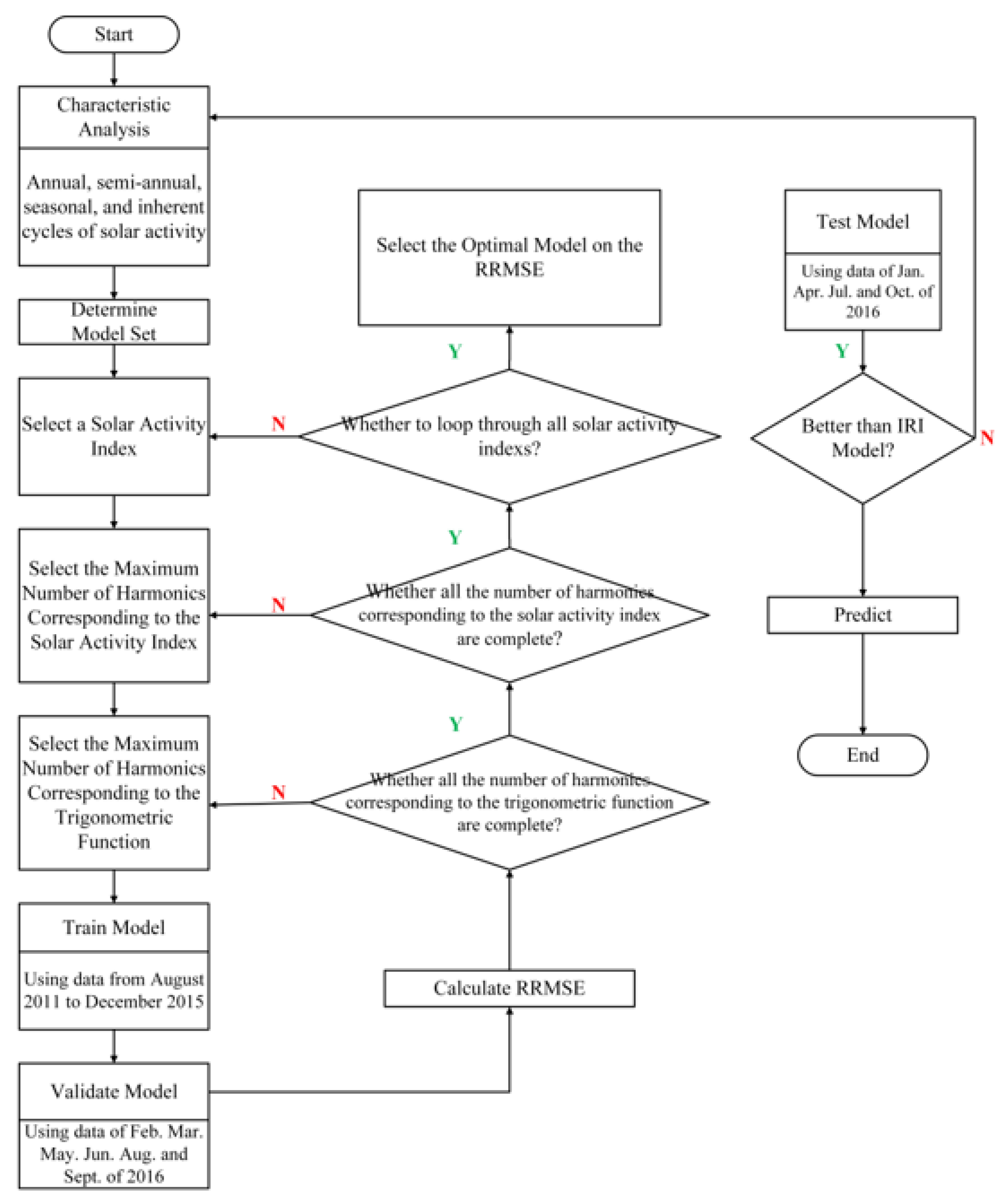
Figure 1. Modeling flowchart based on SML.
Remotesensing 15 03154 g001
Figure 2. hmF2 monthly median data from the Moscow station.
Remotesensing 15 03154 g002
Figure 3. Trend of solar activity index over time.
Remotesensing 15 03154 g003
Figure 4. Prediction model hyperparameter distribution diagram.
Remotesensing 15 03154 g004
Figure 5. Figure comparing observed and verified values: (a) February; (b) March; (c) May; (d) June; (e) August; (f) September.
Remotesensing 15 03154 g005
Figure 6. Comparison observations, and predictions of the IRI and PRO models: (a) January, Winter; (b) April, Spring; (c) July, Summer; (d) October, Autumn.
Remotesensing 15 03154 g006
Figure 7. RMSE and RRMSE obtained by the IRI model and PRO model: (a) RMSE of the model; (b) RMSE calculated by month; (c) RRMSE of the model; (d) RRMSE calculated by month.
Remotesensing 15 03154 g007
Disclaimer/Publisher’s Note: The statements, opinions and data contained in all publications are solely those of the individual author(s) and contributor(s) and not of MDPI and/or the editor(s). MDPI and/or the editor(s) disclaim responsibility for any injury to people or property resulting from any ideas, methods, instructions or products referred to in the content.