Identifying Core Wavelengths of Oil Tree’s Hyperspectral Data by Taylor Expansion

Abstract

The interference of background noise leads to the extremely high spatial complexity of hyperspectral data. Sensitive band selecting is an important task to minimize or eliminate the influence of non-target elements. In this study, Taylor expansion is innovatively used to identify core wavelengths/bands of hyperspectral data. Unlike other traditional methods, this proposed Taylor-CC method considers more local and global information of spectral function to estimate the linear/nonlinear correlation between two wavelengths. Using samples of hyperspectral data with a wavelength range of 350–2500 nm and SPAD for Camellia oleifera, this Taylor-CC method is compared with the traditional PCC method derived from the Pearson correlation coefficient. Using the 240 samples with their different 57 core wavelengths identified by the Taylor-CC method and PCC method, three machine models (i.e., random forest-RF, linear regression-LR, and artificial neural network-ANN) are trained to compare their performances. Their results show that the correlation matrix from the Taylor-CC method represents a clear diagonal pattern with near zero values at most locations away from the diagonal, and all three models confirm that the Taylor-CC method is superior to the PCC method. Moreover, the SPAD spectral response relationship based on machine learning algorithms is constructed, and ANN is the best prediction performance among the three models when using the core wavelengths identified by the Taylor-CC method. The Taylor-CC method proposed in this study not only lays a mathematical foundation for the next analysis of the response mechanism between spectral characteristics and nutrient content of Camellia leaf, but also provides a new idea for the correlation analysis of adjacent spectral bands for hyperspectral signals in many applications.

1. Introduction

Hyperspectral analysis technology, relying on precision remote sensing observation equipment, has established a strategy system for not only mining effective target information from signal alization, complex and changeable fresh leaves or canopy scale background, but also intersecting and integrating a variety of natural basic science and computer software technology. It is a rapidly developing non-destructive monitoring technology in recent years [1,2]. The information carried by spectral curves can not only reflect the composition and content of various constituent substances, but also objectively record the non-target components such as temperature and humidity, surface texture, and organizational structure parameters during observation. Coupled with the intervention of a large amount of background noise, spectral peak overlaps and absorption intensity decreases, thus affecting the estimation accuracy and robustness of the model [3]. In the construction of a hyperspectral estimation model, in order to minimize or eliminate the influence of non-target factors, it has become very important to select appropriate spectral preprocessing and feature transformation to improve signal sensitivity. Relevant processing methods can be divided into two categories according to whether the concentration matrix is involved. The first category is only for spectral matrix spectral processing, and its common methods include centralization, standardization, normalization, smoothing, differential transformation, elementary transformation, multiple scattering correction, continuum removal, and wavelet transformation [4,5]. The second one is to process spectral array data by combining concentration array information, typically including orthogonal signal correction and net analysis signal [6]. When using hyperspectral images to nondestructively monitor wheat seed vigor, Zhang et al., comprehensively compared the difference in estimation accuracy between the original spectra and the treatments after smoothing, mean value centralization, multiple scattering correction, standard normal variable transformation, and Savitzky–Golay first-order and second-order derivatives, respectively [7]. Li et al. used a continuous wavelet transformation to process in situ leaf spectra of summer maize, and then developed a vertical nitrogen distribution prediction model with relatively high accuracy [8]. Although so many pretreatment methods have been developed, there is still no one pretreatment that can guarantee the complete removal of all irrelevant information independently.

At present, it is a common inversion method for hyperspectral analysis technology to establish an analysis model for the properties or composition of targets directly based on the spectral response characteristics or using the wavelength variables after dimension reduction and screening. Early studies were mostly based on multiple quantitative analysis methods of linear regression, such as multiple linear regression, principal component regression (PCR), and partial least square regression (PLSR) [9]. As the range of target content expands, the nonlinear characteristics in the spectral data become more significant. Many scholars have carried out scheme optimization from multiple dimensions. One is to introduce nonlinear terms into PCR or PLSR [10]; and, the other is to classify the target samples first, and then establish a local model by a linear correction method [11]. Zhang et al. used transfer learning to evaluate the chlorophyll content of winter wheat, which effectively proved that the hybrid inversion method based on transfer learning was with good accuracy and robustness [12]. Zhang et al. compared the accuracy of rice nitrogen nutrition monitoring between individual learner and ensemble learner, noticing that ensemble algorithms such as Random Forest (RF), Adaboost and Bagging are suitable for hyperspectral data processing [13]. These models are essentially black-box analysis techniques. There are various mathematical parameters with complex abstraction and unclear physical meaning in the models, which cannot directly provide a clear physical basis. However, empirical or semi-empirical models based on statistical methods have always been unable to solve the universality problem from the physical mechanism level.

On the other hand, Soil and Plant Analyzer Development (SPAD) value represents the relative chlorophyll content of plant leaves. Chlorophyll content is an important parameter to describe plant growth, which can reflect the nutritional stress of plants and indicate growth and senescence as well as other developmental stages. Chlorophyll content is closely related to plant photosynthesis, growth and development, and health status. It is widely used in plant health assessment, vegetation productivity monitoring, crop resource control, and pest control. Therefore, accurate measurement of the plant canopy chlorophyll content and the leaf area index is of great significance for ensuring plant growth, flowering and fruiting, stable and high yield, and avoiding off-season. The traditional methods to detect the chlorophyll content of plant leaves are usually extracted with organic solvents (e.g., acetone and ethanol). They not only consume a lot of time and labor but also result in irreversible damage to the leaves, thus making it difficult to monitor the chlorophyll content in a large area. Hyperspectral remote sensing technology, as a technology emerging in recent years, provides one kind of non-destructive, efficient and low-input monitoring means for Camellia production, avoids the damage to leaves by laboratory chemical analysis methods, saves time and effort, improves monitoring aging, and provides possibilities for real-time monitoring, timely control, and precise guidance for Camellia oleifera fertilization in the next step.

In recent years, domestic and foreign scholars have conducted in-depth research on using hyperspectral data to estimate plant chlorophyll content. However, most of their research objects focused on food crops and vegetable crops such as rice, wheat and corn, and other economic crops such as cotton, sugar cane and sugar beet. There are few studies on the monitoring of the chlorophyll content in economic forests such as Camellia oleifera. Yang et al., proposed a clustering regression method via RF and XG-Boost methods, constructing an in situ SPAD estimation model for winter wheat with an accuracy of more than 0.9 [14]. Based on the hyperspectral data of different planting seasons, Zhang et al., proposed a modified chlorophyll index (MCI) on the basis of the chlorophyll index (CI), and compared it with two other optimized vegetation indexes to establish a partial least squares model based on different varieties and different planting methods [15]. Based on the original spectral data of envelope processing, Yu et al., combined chlorophyll-sensitive bands with the absorption characteristics of water spectral as input variables to estimate SPAD value, and used RF to construct a SPAD hyperspectral estimation model with different input quantities. Their results revealed the spectral response mechanism of different rice varieties and provided a technical method for the high-precision inversion of SPAD value of rice leaves [16].

In this study, after identifying the core wavelengths of spectral data of crown height and chlorophyll content, a SPAD estimation model of Camellia oleifera was established from three machine learning models (i.e., random forest-RF, linear regression-LR, and artificial neutral network-ANN). The specific objectives of this study are: (1) to screen the core wavelengths of the spectrum; (2) to identify the best model from RF, LR, and ANN, and use it as a SPAD inversion model; (3) to provide a basis for the growth regulation of Camellia oleifera in production.

2. Methodology

Some researchers have used the Taylor expansion of log-likelihood functions to reach an analytical approximation of Jackknife connection error, which needs lower computational requirements [17]. Guo et al., proposed an index correlation elimination algorithm based on a feedforward neural network and Taylor expansion, which made up for the defect that most evaluation algorithms do not consider the independence between indices [18]. In addition, Taylor expansion has been applied to image space transformation, which can convert the discrete space of images into a continuous linear space, extending the images in an abstract way [19].

In this study related to hyperspectral signals, as the sample bandwidth of hyperspectral measurements becomes smaller, those discrete reflectance data are more similar to a continuous function of wavelength. Based on Taylor expansion used in smooth functions, a novel method is proposed to estimate the correlation of hyperspectral signal between two wavelengths.

Assuming that there are two nearby wavelengths (i.e., x and y) for a continuous reflectance function f with at least a second-order derivative, their corresponding reflectance measurements at the two locations can be described as

$$f(y)=f(x)+f^{\prime }(x)(y-x)+\frac{1}{2}{f}^{″}(x){(y-x)}^2+o\left({(y-x)}^2\right)$$

(1)

and

$$f(x)=f(y)+f^{\prime }(y)(x-y)+\frac{1}{2}{f}^{″}(y){(x-y)}^2+o\left({(x-y)}^2\right)$$

(2)

Equations (1) and (2) based on Taylor expansion describe mathematically the linear/nonlinear relationship between f(x) and f(y). It leads to a new metric of correlation in this study. The estimated reflectance at y by using the derived information up to the second-order derivative at x is

$$\widehat{f}(y)=f(x)+f^{\prime }(x)(y-x)+\frac{1}{2}{f}^{″}(x){(y-x)}^2$$

(3)

and the estimated reflectance at x by using the derived information up to the second-order derivative at y is

$$\widehat{f}(x)=f(y)+f^{\prime }(y)(x-y)+\frac{1}{2}{f}^{″}(y){(x-y)}^2$$

(4)

The absolute difference between the estimated and the observed reflectance, i.e., $|\widehat{f}(y)-f(y)|$ and $|\widehat{f}(x)-f(x)|$, can be used to measure the strength of the relationship between f(x) and f(y), because the closer is the difference to zero, the more accurate estimation of f(y) (or f(x)) using only the information at x (or y), implying the stronger linear or nonlinear relationship between f(x) and f(y). It also means that a greater difference indicates a weaker relationship. Therefore,

$$c(x,y)=\left\{\begin{array}{cc}1-\frac{1}{2}(|\widehat{f}(x)-f(x)|+|\widehat{f}(y)-f(y)|),& |\widehat{f}(x)-f(x)|+|\widehat{f}(y)-f(y)|\le 2\\ 0,& else\end{array}\right.$$

(5)

can be defined as a correlation metric of reflectance between x and y. It has two important properties: (i) $0\le c(x,y)\le 1$, and (ii) $c(x,y)$ is commutative, i.e., $c(x,y)=c(y,x)$.

Based on Equation (5), the discrete hyperspectral reflectance measurement of one sample (e.g., a tree leaf), i.e., $f(x)=[f(x_1),\cdots ,f(x_N)]\in R^N$, can form a correlation matrix $C(f,x)\in R^{N\times N}$ on N wavelengths, where

$$C(f,x)=\left[\begin{array}{ccc}c(x_1,x_1)& \cdots & c(x_1,x_N)\\ ⋮& \ddots & ⋮\\ c(x_N,x_1)& \cdots & c(x_N,x_N)\end{array}\right]$$

(6)

In practice, C(f, x) shows high-value blocks along its diagonal, because the approximation of f(y) via the Taylor expansion Equation (1) is more accurate if x is closer to y. Therefore, after setting up a certain threshold $T_h\in [0,1]$, such that the elements near the diagonal of C(f, x) can be divided into blocks whose elements are all greater than T_h, i.e., $\min (C_{i:i+n})>T_h$, where

$$C_{i:i+n}=C(f,\left[\begin{array}{c}{x}_i\\ ⋮\\ x_{i+n}\end{array}\right])=\left[\begin{array}{ccc}c(x_i,x_i)& \cdots & c(x_i,x_{i+n})\\ ⋮& \ddots & ⋮\\ c(x_{i+n},x_i)& \cdots & c(x_{i+n},x_{i+n})\end{array}\right]$$

(7)

When T_h is high (e.g., T_h = 0.95), the reflectances of the wavelengths within one block can be considered to be highly correlated, thus any one of the reflectances can represent the rest of them. For example, given a C(f,x) and a T_h, its elements (i.e., wavelengths) near its diagonal are then divided into n blocks (i.e., $C_{1:k_1},C_{k_1+1:k_2},\cdots ,C_{k_{n-1}+1:N}$), and the reflectance of the middle element (i.e., wavelength) of each block can be used to represent all reflectances of the wavelengths within this block. Those n middle wavelengths are $\{{\overline{x}}_l:l=1,\cdots ,n\}=\{x_j:j=\frac{k_{j-1}+k_j}{2}\}$ where $k_0=1,k_n=N$. Thus, the final n selected reflectances are $\{f({\overline{x}}_l),l=1,\cdots ,n\}$, which can represent all original reflectances $\{f(x_i),i=1,\cdots ,N\}$.

The correlation matrix of Equation (6) is based on the reflectance measurement of one sample (i.e., f), so the matrix differs with different samples, resulting in different $\left\{{\overline{x}}_l\right\}$ for different samples. If all M samples (i.e., $\{f^{(m)},m=1,\cdots ,M\}$) with the same wavelengths are from the same or similar sources, and their correlation matrices are $\{C(f^{(m)},x),m=1,\cdots ,M\}$, then their averaged

$$C(\overline{f},x)=\frac{1}{M}{\displaystyle \sum _{m=1}^{M}C(f^{(m)},x)}$$

(8)

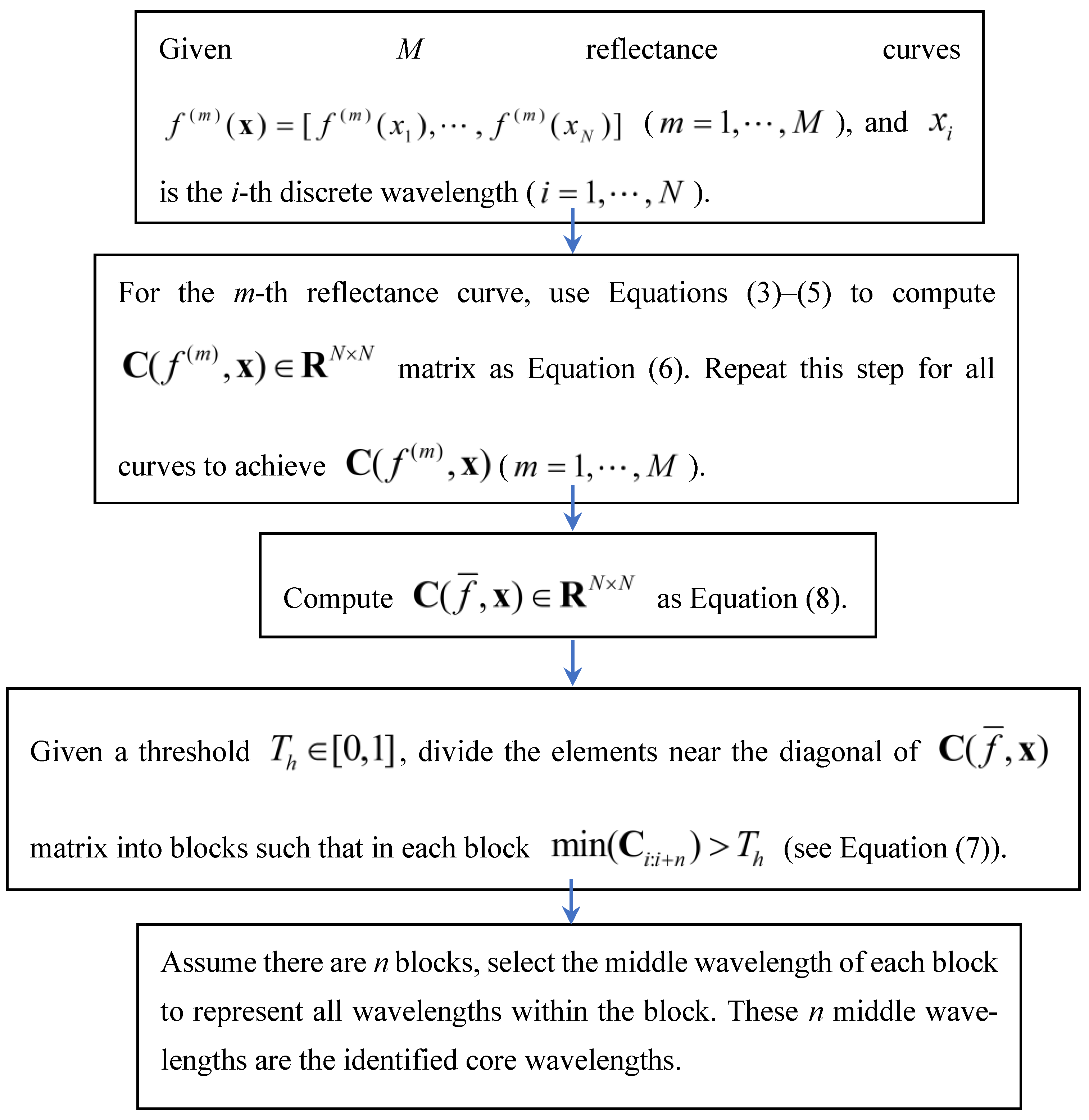
can represent the averaged correlation matrix from these M samples. Equation (8) can then replace Equation (6) to continue subsequence steps (e.g., Equation (7) and its following) for n middle wavelengths $\{{\overline{x}}_l:l=1,\cdots ,n\}$. In the end, these n wavelengths are identified as the core wavelengths of reflectance when using their corresponding reflectances to retrieve other variables such as LAI. The abovementioned new method using $C(\overline{f},x)$ and T_h to identify core wavelengths is based on Taylor expansion, thus it can be called the Taylor-CC method. Appendix A provides a flowchart for using the Taylor-CC method for identifying core wavelengths given a set of reflectance curves.

On the other hand, for a known way to identify core wavelengths using the Pearson Correlation Coefficient (PCC), its correlation matrix of N wavelengths from M samples of reflectance is

$$C_{\overline{f}}(x)=\left[\begin{array}{ccc}\left|c_{\overline{f}}(x_1,x_1)\right|& \cdots & \left|c_{\overline{f}}(x_1,x_N)\right|\\ ⋮& \ddots & ⋮\\ \left|c_{\overline{f}}(x_N,x_1)\right|& \cdots & \left|c_{\overline{f}}(x_N,x_N)\right|\end{array}\right]$$

(9)

where

$$c_{\overline{f}}(x,y)=\frac{1}{M}{\displaystyle \sum _{m=1}^M(f^{(m)}(x)-\overline{f(x)})(f^{(m)}(y)-\overline{f(y)})}$$

and

$$\overline{f(x)}=\frac{1}{M}{\displaystyle \sum _{m=1}^M{f}^{(m)}(x)}$$

Note that $c_{\overline{f}}(x,y)$ comes from PCC. Following similar steps to identify n middle wavelengths of C(f, x) after setting up a certain threshold $T_h\in [0,1]$, these n wavelengths are then identified as the core wavelengths of reflectance based on $C_{\overline{f}}(x)$ and T_h. This core-wavelength identification process can be called the PCC method, which is used in comparison with the Taylor-CC method in the numerical experiments of this study.

3. Machine Learning Models

3.1. Random Forest

RF is an ensemble learning model composed of multiple decision trees [20], which can improve the prediction accuracy and stability of the model. Each decision tree is constructed based on random samples and random features, and this randomness enables RF to avoid overfitting.

Depending on whether each tree is a classification tree or a regression tree, RF can be applied to classification or regression problems, respectively. In the regression analysis by RF, there are two key parameters, i.e., ntree and mytry. ntree is the number of decision trees, and mytry is the number of random features. In this study, the value of ntree was set to 5, and mytry was the default value in the treebagger function [21].

The algorithm of RF is described in the following steps [22]. First of all, given N total training samples, using bootstrap sampling, a single decision tree randomly selects n samples from the N training samples as the training samples of this single tree. Then, when splitting at each node of each decision tree, m input features are randomly selected from mytry features, where m < mytry. Using n samples and m input features, a complete decision tree is finally learned, and a random forest is achieved.

3.2. Linear Regression

The mathematical expression of linear regression is $\mathrm{y}={\beta }_0+{\beta }_1{x}_1+{\beta }_2{x}_2+\cdots +{\beta }_n{x}_n$, where ${\beta }_0, {\beta }_1, {\beta }_2\cdots {\beta }_n$ are the regression coefficients, and $x_1, x_2\cdots x_n$ are predictor variables. The values of ${\beta }_0, {\beta }_1, {\beta }_2\cdots {\beta }_n$ are determined by the model and least square fit.

3.3. Artificial Neural Network

ANN is a research hotspot in the field of artificial intelligence since the 1980s [23]. It is widely used in physical and chemical properties screening [24], vulnerability assessment [25], river flow prediction [26], and other specific fields. It is an operational model consisting of a large number of nodes connected to each other. Each node represents a specific output function, called the activation function. The connection between each pair of nodes represents a weighted value for the signal through the connection, called weight.

Information is first processed layer by layer from the input layer to the hidden layer, and the output result of the output layer is compared with the expected value. When the error between the output layer and the expected value is greater than the predetermined value, backward propagation will be performed. Then, weights and thresholds of the network are adjusted according to the prediction error, and the network transfer is propagated forward [27].

In this study, because the number of 240 samples is not large, 15 hidden nodes and up to 3 hidden layers were used to identify a suitable ANN structure. In the end, the most suitable network structure is determined to be 13 × 2 of hidden nodes by analyzing model performance to predict SPAD under different structures [28].

4. Data and Experiments

4.1. Overview of the Study Area

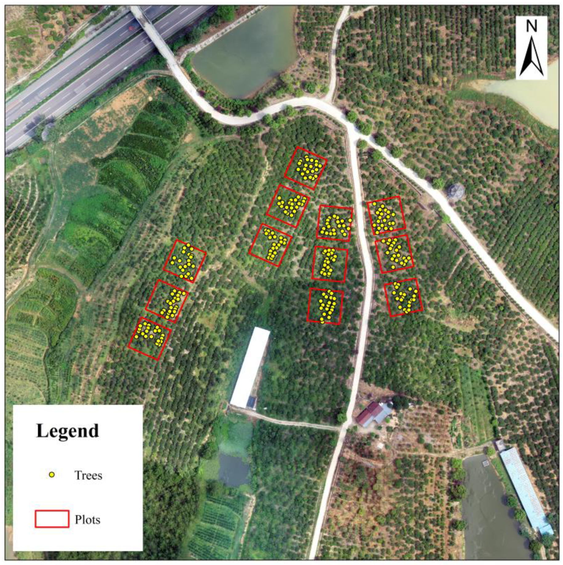
The experimental study area of collected data is located in Huangpu Town, Qianshan City, Anhui Province (Figure 1). It is in the southern periphery of Dabie Mountains, with high terrain in the northwest and low in the southeast. The northwest part of the terrain is mountainous, and the rest is hilly. Huangpu Town has a subtropical monsoon climate, which is characterized by four distinct seasons: mild spring and autumn climate, hot summer, and dry and cold winter. Rain is abundant throughout years.

4.2. Design of Site Experiments

The test site is located in Jinghui Camellia Professional Cooperative in Qianshan County, Anhui Province. From 31 July to 6 August 2022, 12 square plots of 20 m × 20 m were set up in the study area, and 20 trees were selected in each plot, with a total of 240 plants. All trees studied in this experiment are Changlin series Camellia oleifera that have entered a stable fruit production period. They provided a series of measurement data such as canopy hyperspectral data and SPAD.

4.3. Hyperspectral Data Acquisition

In this study, an all-band terrain spectrometer (Fieldspec4 Wide-Res, Analytical Spectrum Devices Inc., Boulder, CO, USA) was used to obtain the canopy spectrum of 240 trees in the study area, with a wavelength range of 350–2500 nm. The fiber optic cable of the spectrometer was raised above the center of the plant canopy through the fiber jumper, fiber adapter, carbon fiber telescopic rod, and pipeline clamp (the fiber optic probe is perpendicular to the top of the canopy), and a circular observation area with a diameter ($D=2\ast h\ast tan12.5°$, h is the vertical distance between the fiber optic probe and the center of the canopy) was formed. All measurements were carried out under the conditions of sunny weather, no wind and no cloud, and the solar altitude angle greater than 45°. It was usually from 10 am to 2 pm in local time. The surveyors dressed themselves in dark clothes, faced the sun when measuring, and kept a certain distance from the edge of the plant canopy, so as to avoid the influence of shadow and human disturbance on the canopy spectra collection. The instrument was preheated for at least 20 min before measuring, and whiteboard correction was performed. Each sample was measured 10 times continuously, and the average values were taken as the original canopy spectra of the sample.

4.4. SPAD Data Acquisition

SPAD-502 plus chlorophyll meter (SPAD-502 plus, Konica Minolta, Inc., Osaka, Japan) is a widely used instrument for measuring the relative content of chlorophyll in plant leaves. The meter was used to determine the relative chlorophyll content of Camellia oleifera leaves. It determines the relative chlorophyll content of a leaf by measuring the optical concentration difference (transmittance) of the leaf at two wavelengths (650 nm and 940 nm). In order to ensure the coincidence with the hyperspectral observation scale, the spatial position of measured leaves should be in a circular area with a diameter of 0.9 m and the center of the upper surface of their canopy. When collecting leaves, the leaves with the upper surface facing the sky should be selected as much as possible. During collection, the samples should be evenly sampled in the four directions of the plant. The number of leaves should be at least 16, and each leaf took three SPAD measurements, so a plant should take at least 48 measurements. The 48 values were averaged to calculate the SPAD measurement of the leaves on the upper surface of the canopy of a single plant after eliminating outliers.

4.5. Measurements

240 hyperspectral measurement samples are pre-processed to remove invalid data outside [0, 1]. Their cleaned data set are shown in Figure 2a, whose broken/blank parts are due to the invalid data. On the other hand, the histogram of SPAD data corresponding to the 240 measurement samples is shown in Figure 2b, similar to a bell shape from Normal distribution.

4.6. Numerical Experiment Setup and Purposes

Using the 240 samples with their different 57 core wavelengths identified by the Taylor-CC and the PCC method, three machine models (i.e., RF, linear regression, and ANN) were trained to compare their performances. In this study, all input/output data (i.e., reflectance and SPAD) were scaled onto [−1, 1], so as to reduce the adverse effects caused by the singular sample data. Then, 70%/30% (i.e., 168/72) samples were randomly selected as the training/testing samples in RF and linear regression. Due to the model requirements of ANN, these 240 samples were randomly divided into three parts, i.e., training samples, validation samples and testing samples, with a ratio of 70%/15%/15%, respectively. The training sample of ANN are used as the training samples of both RF and linear regression, while the union of validation and testing samples become the testing samples of both RF and linear regression.

In addition to comparing the performances of the three models, it is also necessary to compare the proposed Taylor-CC method and PCC method of screening wavelengths, so as to illustrate the advantages of the new Taylor-CC method over the ordinary PCC method to a certain extent. In both methods, different numbers of core wavelengths can be obtained by setting different thresholds. However, to ensure the validity of the comparison results of both methods, the same number of obtained core wavelengths needed to be used in both methods. Therefore, in the numerical experiments of this study, both methods use the same number of core wavelengths by setting different thresholds, but both sets of wavelengths are normally different.

4.7. Evaluation Metrics

Cross-validation is needed to assess the performance of the three machine models, as well as that of both methods. In this study, root mean square error (RMSE), determination coefficient (R²), mean absolute error (MAE), mean square error (MSE), mean bias error (MBE), percentage bias error (PBE), relative absolute error (RAE), relative mean absolute error (RMAE), and Nash and Sutcliffe’s model efficiency (NSE) are used as the metrics to evaluate models and methods. They are defined as

$$\mathrm{RMSE}=\sqrt{\frac{1}{N}{\displaystyle \sum }_{i=1}^N{\left(y_i-x_i\right)}^2}$$

$$R^2=\frac{{\left({\sum }_{i=1}^N\left(x_i-\overline{x}\right)\left(y_i-\overline{y}\right)\right)}^2}{{\sum }_{i=1}^N{\left(x_i-\overline{x}\right)}^2{\sum }_{i=1}^N{\left(y_i-\overline{y}\right)}^2}$$

$$\mathrm{MAE}=\frac{1}{N}{\displaystyle \sum }_{i=1}^N\left|y_i-x_i\right|$$

$$\mathrm{MSE}=\frac{1}{N}{\displaystyle \sum }_{i=1}^N{\left(y_i-x_i\right)}^2$$

$$\mathrm{MBE}=\frac{1}{N}{\displaystyle \sum }_{i=1}^N\left(x_i-y_i\right)$$

$$\mathrm{PBE}=100\frac{{\sum }_{i=1}^N\left(y_i-x_i\right)}{{\sum }_{i=1}^N{x}_i}$$

$$\mathrm{RAE}=\frac{{\sum }_{i=1}^N\left|y_i-x_i\right|}{{\sum }_{i=1}^N\left|x_i-\overline{x}\right|}$$

$$\mathrm{RMAE}=\frac{1}{N}\frac{{\sum }_{i=1}^N\left|y_i-x_i\right|}{\overline{x}}$$

$$\mathrm{NSE}=1-\frac{\frac{1}{N}{\sum }_{i=1}^N{\left(y_i-x_i\right)}^2}{\frac{1}{N}{\sum }_{i=1}^N{\left(x_i-\overline{x}\right)}^2}$$

where $x_i$ is the i-th observed value, $y_i$ is the i-th model predicted value, N is the size of x and y, $\overline{x}$ is the average of x, and $\overline{y}$ is the average value of y. Model performs better when RMSE, MAE, MSE, RAE or RMAE is smaller, R² is higher, MBE or PBE is closer to zero, or NSE is closer to one.

5. Results

5.1. Correlation Matrices from the Taylor-CC Method and the PCC Method

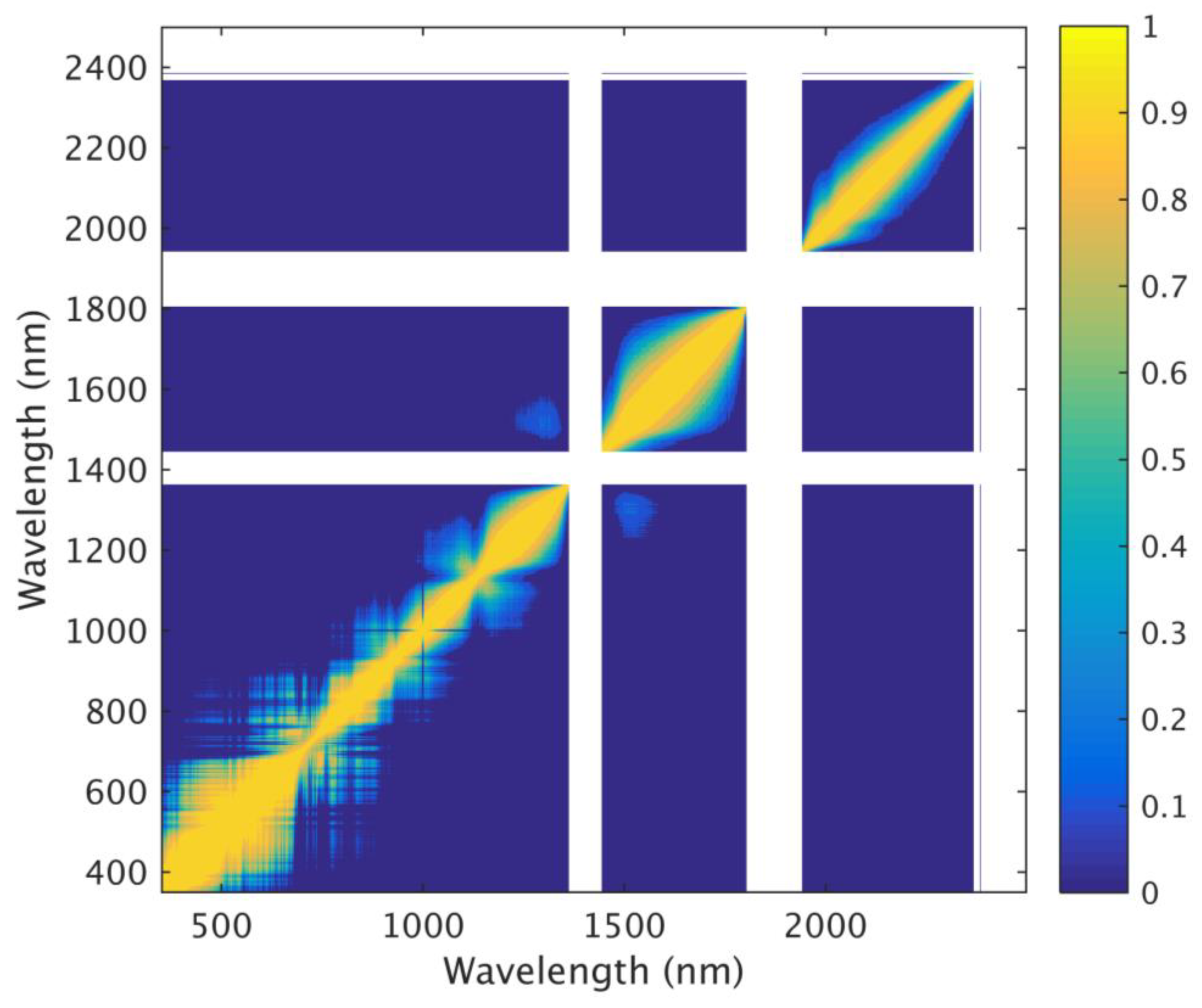
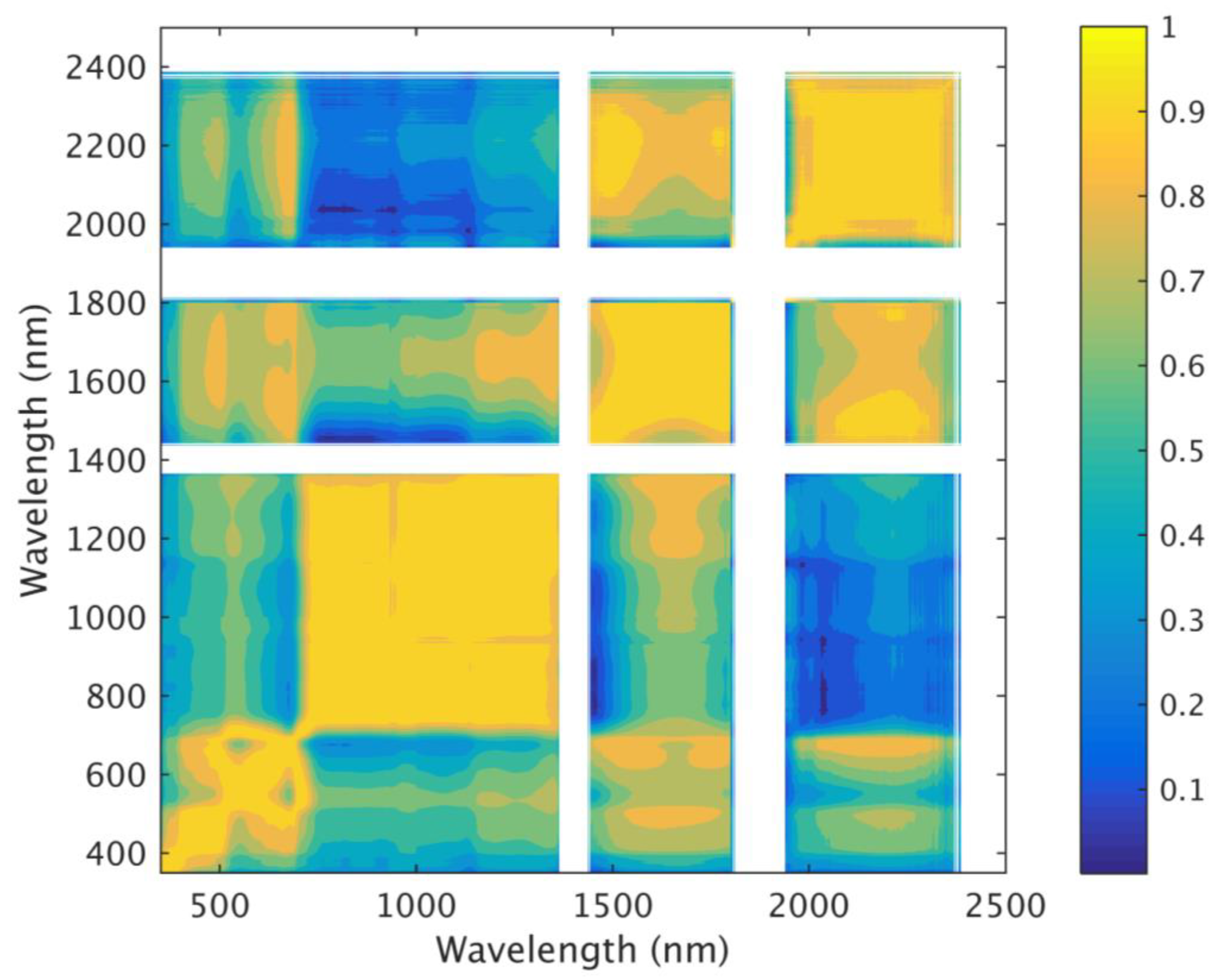
Using the 240 reflectance measurements in Figure 2a, $C(\overline{f},x)$ of the Taylor-CC method and $C_{\overline{f}}(x)$ of the PCC method are shown in Figure 3 and Figure 4, respectively. $C(\overline{f},x)$ of Taylor-CC shows a clear diagonal pattern with near zero values at most locations away from the diagonal. It is reasonable in most applications. On the other hand, although $C_{\overline{f}}(x)$ of PCC also shows diagonal pattern, its off-diagonal locations also occupied with many high values, even at the locations far away from the diagonal. Those off-diagonal high values are unreasonable unless the reflectance function f(x) is similar to a periodic function.

5.2. Identifying Core Wavelengths

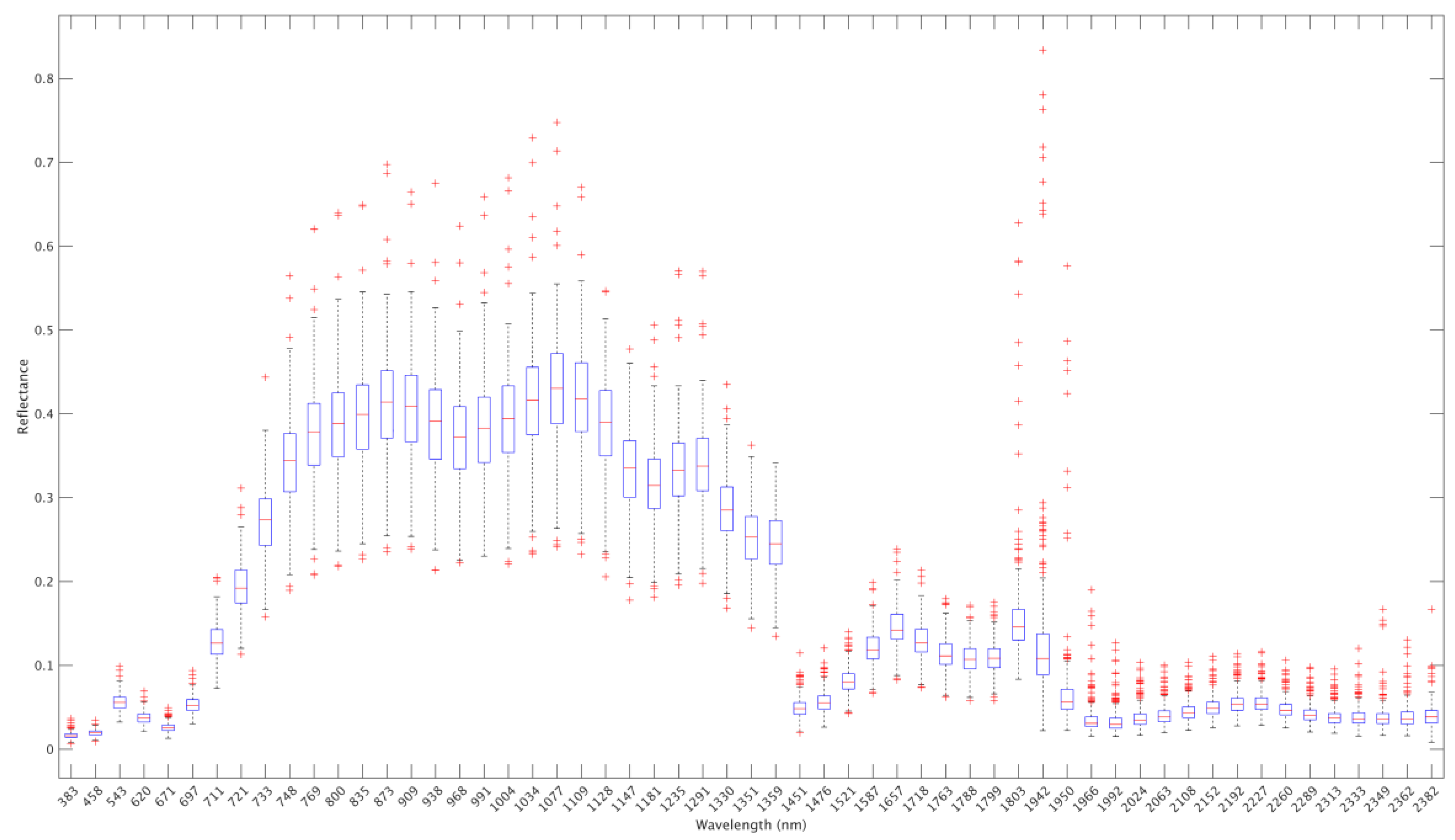
Both the Taylor-CC method and the PCC method can identify different number of core wavelengths based on different threshold T_h, therefore, the same number of core wavelengths from the two methods are required, so that both methods can be benchmarked and compared. The T_h threshold of the Taylor-CC method was set to 0.872, and 57 wavelengths were screened. At the same time, to achieve 57 wavelengths in the PCC method, its T_h threshold was set as 0.934. Both sets of wavelengths are presented in Figure 5, and the selected 57 wavelengths from the Taylor-CC method is provided in Appendix B. It shows a more even distributed pattern along the wavelength domain for the Taylor-CC method than that for the PCC method, implying that the Taylor-CC method is trying to capture input information along the domain evenly, while the PCC method results in some large blank wavelength gaps and dense parts at high wavelengths. In addition, some important reflectance statistics of the selected 57 wavelengths from the Taylor-CC method are presented in Appendix C.

These two sets of obtained wavelengths with the same number (i.e., 57) will be passed into three different machine learning models (i.e., RF, linear regression, and ANN). Thus, (i) the Taylor-CC method can be verified to be superior to the PCC method, and (ii) the best model among the three can be selected as the best SPAD retrieval model.

5.3. Model Evaluation Using Two Methods

Using two sets of 57 core wavelengths identified by the Taylor-CC and PCC methods, together with the 240 samples including reflectance and SPAD, two models (i.e., RF and linear regression) carried out training and testing, and one model (i.e., ANN) went through training, testing, and validation.

The results of RF are listed in

Table 1. Performance assessments of RF.

	PCC Method		Taylor-CC Method
	Training	Testing	Training	Testing
RMSE	0.2443	0.4335	0.2283	0.4149
R2	0.6190	0.0338	0.6740	0.1012
MAE	0.1826	0.3554	0.1712	0.3326
MSE	0.0597	0.1879	0.0521	0.1721
MBE	−0.0034	−0.0044	−0.0082	−0.0040
PBE	5.62%	10.22%	13.67%	9.31%
RAE	0.6060	1.0299	0.5679	0.9637
RMAE	3.0362	8.2337	2.8452	7.7044
NSE	0.5821	−0.0256	0.6351	0.0607

. In the training, the values of the nine metrics in both methods are similar. In the testing, it is clear that the values of all nine metrics in the Taylor-CC method are better than those in the PCC method, which indicates that the Taylor-CC method is superior to the PCC method in the RF model, with low RMSE, high R², low MAE, low MSE, MBE close to zero, PBE close to zero, low RAE, low RMAE, and NSE close to one. Note that in the RF experiments, five trees are established, and the maximum depth is 15.

The results of linear regression are listed in

Table 2. Performance assessments of linear regression.

	PCC Method		Taylor-CC Method
	Training	Testing	Training	Testing
RMSE	0.2438	0.6427	0.2319	0.3874
R2	0.5838	0.0804	0.6236	0.3403
MAE	0.1907	0.3585	0.1838	0.2893
MSE	0.0594	0.4131	0.0538	0.1501
MBE	0.0000	0.0234	−0.0000	0.0016
PBE	−0.00%	−54.15%	0.00%	−3.81%
RAE	0.6328	1.0388	0.6099	0.8384
RMAE	3.1705	8.3053	3.0557	6.7025
NSE	0.5838	−1.2543	0.6236	0.1811

. In the training, the values of the nine metrics in both methods are still similar. However, in the testing, all nine metrics in the Taylor-CC method are much better than those in the PCC method. Therefore, a more convincing conclusion can be drawn that the performance of the Taylor-CC method is better than that of the PCC method in linear regression model.

The results of ANN are listed in

Table 3. Performance assessments of ANN.

	PCC Method		Taylor-CC Method
	Training	Testing	Training	Testing
RMSE	0.3838	0.4400	0.2547	0.3058
R2	0.4984	0.3546	0.5880	0.4667
MAE	0.3212	0.3559	0.2005	0.2411
MSE	0.1473	0.1936	0.0649	0.0935
MBE	0.2744	0.2959	0.0675	0.1070
PBE	−456.19%	−447.32%	−112.24%	−161.77%
RAE	1.0656	1.1446	0.6653	0.7755
RMAE	5.3387	5.3813	3.3333	3.6459
NSE	−0.0311	−0.3015	0.5458	0.3714

. Note that the testing results are actually from the combination of the testing and validation results of ANN. From the nine metrics obtained in the training and testing, it is obvious that the metrics are all much better in the Taylor-CC method than in the PCC method. It implies that the Taylor-CC method could work the best for ANN among the three models, although ANN could introduce some bias.

With the conclusion that the Taylor-CC method is better than the PCC method, focus is shifted to identify the best model for the Taylor-CC method. Thus, using only the Taylor-CC method, one could focus on the model performance with all the samples (i.e., 240) (see

Table 4. Performance assessments of RF, linear regression, and ANN using all the samples.

	RF	Linear Regression	ANN
RMSE	0.2968	0.2875	0.2711
R2	0.4369	0.4928	0.5358
MAE	0.2196	0.2155	0.2127
MSE	0.0881	0.0827	0.0735
MBE	−0.0070	0.0005	0.0794
PBE	12.65%	−0.9%	−128.1%
RAE	0.6978	0.6847	0.6992
RMAE	3.9881	3.9134	3.4334
NSE	0.4316	0.4668	0.4920

), as well as that with only the testing samples (i.e., 240 × 30% = 72) (see

Table 5. Performance assessments of RF, linear regression, and ANN using only the testing samples.

	RF	Linear Regression	ANN
RMSE	0.4149	0.3874	0.3058
R2	0.1012	0.3403	0.4667
MAE	0.3326	0.2893	0.2411
MSE	0.1721	0.1501	0.0935
MBE	−0.0040	0.0016	0.1070
PBE	9.31%	−3.81%	−161.77%
RAE	0.9637	0.8384	0.7755
RMAE	7.7044	6.7025	3.6459
NSE	0.0607	0.1811	0.3714

). The performance comparison with all the samples shows that RF and linear regression are similar, but ANN is better than both of them in terms of RMSE, R², MAE, MSE, RMAE, and NSE. On the other hand, the performance comparison with only the testing samples shows that RF and linear regression are still similar, but ANN is much better than both of them except for MBE and PBE. It indicates that ANN may only work a bit better than the other two methods during training, but its predictive ability during testing works much better than the other two methods. It concludes that ANN with the Taylor-CC method is the best performance in this study, although ANN could introduce some bias.

6. Discussion

In this paper, a new method based on Taylor expansion is proposed to estimate the correlation of hyperspectral signals between two wavelengths, so as to identify the core bands of hyperspectral data. It is known that a large number of spectral bands of hyperspectral remote sensing data provide very rich remote sensing information. However, due to the continuity of wavelength bands in hyperspectral data, the high correlation between different bands, and the serious redundancy of band information, it is unnecessary to use all the bands’ information [29], which could result in extra weights on those redundant bands or too many computations in retrieval. The data mining process of hyperspectral data is essentially to solve typical high-dimensional problems. When the number of samples is much less than the dimension of spectral data, it may face the ’dimension disaster’, which indirectly leads to the reduction in analysis accuracy. In order to address this problem, three types of processing methods have been proposed by researchers, namely regularization, data dimensionality reduction, and variable selection [30]. The commonly used regularization methods include ridge regression, LASSO regression, etc. [31]. Data dimensionality reduction methods include PCA and PLS [32]. Although those methods can effectively reduce the influence of multicollinearity, the effect is often poor when irrelevant information or noise dominates. Variable selection of those methods is based on a specific wavelength or wavelength interval. Although their variable-selection results can simplify models and could reach a robust and explanatory estimation model [33], their ideas are still limited onto the discrete values of variables instead of a more global picture.

In this study, Taylor expansion, a classical mathematical tool for continuous functions, is used innovatively to discover the linear or nonlinear correlation between two bands, especially two nearby bands. This new method, for the first time, treats hyperspectral data as continuous functions, so that the value of one function at one wavelength can be approximated by another value of the function at another wavelength under strict mathematical derivations. Moreover, this method can not only utilize the multiple pieces of local information at one wavelength (i.e., different orders of derivatives) but also introduce the distance between this wavelength and a target wavelength, making this method more like a global method, which has not been achieved by all other methods to identify core wavelengths.

On the other hand, the real recognition significance of the ground object spectrum is a series of spectral absorption features in spectral–complete curves. The position and shape information of these absorption features are closely related to the material properties and environmental factors. This research focuses on wavelength/band selection as mathematical problems, and future research should pay more attention to the physical meaning of those combinations of wavelengths.

7. Conclusions

In this study, a new method named the Taylor-CC method is proposed to estimate the linear/nonlinear correlation between two wavelengths of hyperspectral signals. The proposed method and the known PCC method are also compared in this study. The wavelength-relevant correlation matrix $C(\overline{f},x)$ from the Taylor-CC method shows a clear diagonal pattern with near-zero values at most locations away from the diagonal. It makes obvious sense in most applications. Using the 240 samples with their different 57 core wavelengths identified by the Taylor-CC method and the PCC method, three machine models (i.e., RF, linear regression, and ANN) were trained to compare their performances. All three models confirmed that the Taylor-CC method is superior to the PCC method (see Table 1, Table 2 and Table 3). The SPAD spectral response relationship based on machine learning was further constructed, and results showed that ANN was the best prediction performance (RMSE = 0.3058, R² = 0.4667, MAE = 0.2411, MSE = 0.0935, RAE = 0.7755, RMAE = 3.6459, and NSE = 0.3714) among the three models when using the core wavelengths from the Taylor-CC method. Although the ANN model could introduce some bias in its prediction, some possible ways to reduce or remove the bias can be taken so as to further improve its prediction accuracy. For example, adding an additional input-dependent bias function or network into the ANN.

The Taylor expansion method used in this study provides a new idea for the correlation analysis of adjacent spectral intervals, which lays a mathematical foundation for the further analysis of the response mechanism between spectral characteristics and nutrient content. Furthermore, this method could be used in other applications/fields with hyperspectral signals/images, which can be treated as continuous functions in spectral space. Although some particular hyperspectral signals are obviously discontinuous and cannot be directly applied to the Taylor-CC method, they can still be viewed as piecewise functions and apply the method to each interval with a continuous function.

References

1. Zhao, D.; Li, J.; Song, Z. Hyperspectral remote sensing for estimating biochemical variables of canopy. Adv. Earth Sci. 2003, 1, 94–99. [Google Scholar]
2. Ma, B.; Yu, G.; Wang, W.; Luo, X.; Li, Y.; Li, X.; Lei, S. Recent advances in spectral analysis technique for non-destructive detection of internal quality in watermelon and muskmelon: A review. Spectrosc. Spectral Anal. 2020, 7, 2035–2041. [Google Scholar] [CrossRef]
3. Yang, C.; Feng, M.; Song, L.; Jing, B.; Xie, Y.; Wang, C.; Song, X. Study on hyperspectral monitoring model of soil total nitrogen content based on fractional-order derivative. Comput. Electron. Agric. 2022, 201, 107307. [Google Scholar] [CrossRef]
4. Mezned, N.; Alayet, F.; Dkhala, B.; Abdeljaouad, S. Field hyperspectral data and OLI8 multispectral imagery for heavy metal content prediction and mapping around an abandoned Pb–Zn mining site in northern Tunisia. Heliyon 2022, 6, e09712. [Google Scholar] [CrossRef]
5. Zhao, R.; An, L.; Tang, W.; Gao, D.; Qiao, L.; Li, M.; Qiao, J. Deep learning assisted continuous wavelet transform-based spectrogram for the detection of chlorophyll content in potato leaves. Comput. Electron. Agric. 2022, 195, 106802. [Google Scholar] [CrossRef]
6. Xie, L.; Hong, M.; Yu, Z. A wavelength selection method combing direct orthogonal signal correction and monte carlo. Spectrosc. Spectr. Anal. 2022, 2, 440–445. [Google Scholar] [CrossRef]
7. Zhang, T.; Fan, S.; Xiang, Y.; Sun, Q. Non-destructive analysis of germination percentage, germination energy and simple vigour index on wheat seeds during storage by Vis/NIR and SWIR hyperspectral imaging. Spectrochim. Acta Part A 2020, 239, 118488. [Google Scholar] [CrossRef]
8. Li, L.; Geng, S.; Lin, D.; Su, G.; Zhang, Y.; Chang, L.; Wang, L. Accurate modeling of vertical leaf nitrogen distribution in summer maize using in situ leaf spectroscopy via CWT and PLS-based approaches. Eur. J. Agron. 2022, 140, 126607. [Google Scholar] [CrossRef]
9. Li, L.; Liu, G.; Fan, N.; He, J.; Li, Y.; Sun, Y.; Pu, F. A combination of hyperspectral imaging with two-dimensional correlation spectroscopy for monitoring the hemicellulose content in Lingwu long jujube. Spectrosc. Spectral Anal. 2022, 12, 3935–3940. [Google Scholar] [CrossRef]
10. Elliott, K.W.; Delaglio, F.; Wikström, M.; Marino, J.P.; Arbogast, L.W. Principal Component Analysis of 1D 1H Diffusion Edited NMR Spectra of Protein Therapeutics. J. Pharm. Sci. 2021, 10, 3385–3394. [Google Scholar] [CrossRef]
11. St. Luce, M.; Ziadi, N.; Viscarra Rossel, R.A. GLOBAL-LOCAL: A new approach for local predictions of soil organic carbon content using large soil spectral libraries. Geoderma 2022, 425, 116048. [Google Scholar] [CrossRef]
12. Zhang, Y.; Hui, J.; Qin, Q.; Sun, Y.; Zhang, T.; Sun, H.; Li, M. Transfer-learning-based approach for leaf chlorophyll content estimation of winter wheat from hyperspectral data. Remote Sens. Environ. 2021, 267, 112724. [Google Scholar] [CrossRef]
13. Zhang, J.; Xu, B.; Feng, H.; Jing, X.; Wang, J.; Ming, S.; Fu, Y. Monitoring nitrogen nutrition and grain protein content of rice based on ensemble learning. Spectrosc. Spectral Anal. 2022, 6, 1956–1964. [Google Scholar] [CrossRef]
14. Yang, X.; Yang, R.; Ye, Y.; Yuan, Z.; Wang, D.; Hua, K. Winter Wheat SPAD Estimation from UAV Hyperspectral Data Using Cluster-Regression Methods. Int. J. Appl. Earth Obs. 2021, 105, 102618. [Google Scholar] [CrossRef]
15. Zhang, J.; Tian, H.; Wang, D.; Li, H.; Mouazen, A.M. A Novel Spectral Index for Estimation of Relative Chlorophyll Content of Sugar Beet. Comput. Electron. Agric. 2021, 184, 106088. [Google Scholar] [CrossRef]
16. Yu, Z.; Zhang, X.; Liu, H.; Zhang, Z.; Meng, L.; Han, Y.; Lu, L. Improving SPAD Spectral Estimation Accuracy of Rice Leaves by Considering the Effect of Leaf Water Content. Crop Sci. 2022, 62, 2382–2395. [Google Scholar] [CrossRef]
17. Robitzsch, A. Analytical Approximation of the Jackknife Linking Error in Item Response Models Utilizing a Taylor Expansion of the Log-Likelihood Function. AppliedMath 2023, 3, 49–59. [Google Scholar] [CrossRef]
18. Guo, W.; Qiu, H.; Liu, Z.; Zhu, J.; Wang, Q. An Integrated Model Based on Feedforward Neural Network and Taylor Expansion for Indicator Correlation Elimination. Intell. Data Anal. 2022, 26, 751–783. [Google Scholar] [CrossRef]
19. Fu, F.; Fang, M.; Yang, H.; Li, Z. High-Order Taylor Expansion Based Image Space Transform Method for Real-Time Augmented Reality. Comput. Commun. 2020, 153, 294–301. [Google Scholar] [CrossRef]
20. Segal, M.R. Machine learning benchmarks and random forest regression. Cent. Bioinforma. Mol. Biostat. Univ. Calif. San Franc. 2004. Available online: https://escholarship.org/uc/item/35x3v9t4 (accessed on 15 April 2023).
21. Svetnik, V.; Liaw, A.; Tong, C.; Culberson, J.C.; Sheridan, R.P.; Feuston, B.P. Random Forest:  A Classification and Regression Tool for Compound Classification and QSAR Modeling. J. Chem. Inf. Comput. Sci. 2003, 43, 1947–1958. [Google Scholar] [CrossRef] [PubMed]
22. Rodriguez-Galiano, V.; Sanchez-Castillo, M.; Chica-Olmo, M.; Chica-Rivas, M. Machine Learning Predictive Models for Mineral Prospectivity: An Evaluation of Neural Networks, Random Forest, Regression Trees and Support Vector Machines. Ore Geol. Rev. 2015, 71, 804–818. [Google Scholar] [CrossRef]
23. Abiodun, O.I.; Jantan, A.; Omolara, A.E.; Dada, K.V.; Mohamed, N.A.; Arshad, H. State-of-the-Art in Artificial Neural Network Applications: A Survey. Heliyon 2018, 4, e00938. [Google Scholar] [CrossRef] [PubMed] [Green Version]
24. Ciura, K.; Kovačević, S.; Pastewska, M.; Kapica, H.; Kornela, M.; Sawicki, W. Prediction of the Chromatographic Hydrophobicity Index with Immobilized Artificial Membrane Chromatography Using Simple Molecular Descriptors and Artificial Neural Networks. J. Chromatogr. A 2021, 1660, 462666. [Google Scholar] [CrossRef] [PubMed]
25. Afsari, R.; Nadizadeh Shorabeh, S.; Bakhshi Lomer, A.R.; Homaee, M.; Arsanjani, J.J. Using Artificial Neural Networks to Assess Earthquake Vulnerability in Urban Blocks of Tehran. Remote Sens. 2023, 15, 1248. [Google Scholar] [CrossRef]
26. Burgan, H.I. Comparison of different ANN (FFBP GRNN RBF) algorithms and multiple linear regression for daily streamflow prediction in Kocasu river—Turkey. Fresen. Environ. Bull. 2022, 31, 4699–4708. [Google Scholar]
27. Dong, L.; Du, H.; Han, N.; Li, X.; Zhu, D.; Mao, F.; Zhang, M.; Zheng, J.; Liu, H.; Huang, Z.; et al. Application of Convolutional Neural Network on Lei Bamboo Above-Ground-Biomass (AGB) Estimation Using Worldview-2. Remote Sens. 2020, 12, 958. [Google Scholar] [CrossRef] [Green Version]
28. Cabaneros, S.M.; Calautit, J.K.; Hughes, B.R. A Review of Artificial Neural Network Models for Ambient Air Pollution Prediction. Environ. Model. Softw. 2019, 119, 285–304. [Google Scholar] [CrossRef]
29. Reshma, R.; Sowmya, V.; Soman, K.P. Dimensionality Reduction Using Band Selection Technique for Kernel Based Hyperspectral Image Classification. Procedia Comput. Sci. 2016, 93, 396–402. [Google Scholar] [CrossRef] [Green Version]
30. Yun, Y.; Li, H.; Deng, B.; Cao, D. An overview of variable selection methods in multivariate analysis of near-infrared spectra. Trac-Trend. Anal. Chem. 2019, 113, 102–115. [Google Scholar] [CrossRef]
31. Tateishi, S.; Matsui, H.; Konishi, S. Nonlinear regression modeling via the lasso-type regularization. J. Stat. Plan. Infer. 2009, 5, 1125–1134. [Google Scholar] [CrossRef]
32. Das, B.; Manohara, K.K.; Mahajan, G.R.; Sahoo, R.N. Spectroscopy based novel spectral indices, PCA- and PLSR-coupled machine learning models for salinity stress phenotyping of rice. Spectrochim. Acta Part A 2020, 229, 117983. [Google Scholar] [CrossRef]
33. Kamruzzaman, M.; Kalita, D.; Ahmed, M.T.; ElMasry, G.; Makino, Y. Effect of variable selection algorithms on model performance for predicting moisture content in biological materials using spectral data. Anal. Chim. Acta 2022, 1202, 339390. [Google Scholar] [CrossRef]
Figure 1. Overview of the study area.
Remotesensing 15 03137 g001
Figure 2. (a) 240 hyperspectral measurement samples after removing invalid reflectance (Note: color is only for distinguishing different lines and has no other meaning), and (b) the distribution of their SPAD measurements.
Remotesensing 15 03137 g002aRemotesensing 15 03137 g002b
Figure 3. The correlation matrix  C ( f ¯ , x )  from the Taylor-CC method.
Remotesensing 15 03137 g003
Figure 4. The correlation matrix  C f ¯ ( x )  from the PCC method.
Remotesensing 15 03137 g004
Figure 5. Core wavelengths identified via the PCC method and the Taylor-CC method. They are 57 wavelengths for each method with different thresholds.
Remotesensing 15 03137 g005