Review

A Review of Hyperspectral Image Super-Resolution Based on Deep Learning

1
Changchun Institute of Optics, Fine Mechanics and Physics, Chinese Academy of Sciences, Changchun 130033, China
2
University of Chinese Academy of Sciences, Beijing 100049, China
3
Department of Electronic Engineering, Tsinghua University, Beijing 100084, China
*
Author to whom correspondence should be addressed.
Remote Sens. 2023, 15(11), 2853; https://doi.org/10.3390/rs15112853
Submission received: 31 March 2023 / Revised: 18 May 2023 / Accepted: 27 May 2023 / Published: 31 May 2023

Abstract

:
Hyperspectral image (HSI) super-resolution (SR) is a classical computer vision task that aims to accomplish the conversion of images from lower to higher resolutions. With the booming development of deep learning (DL) technology, more and more researchers are dedicated to the research of image SR techniques based on DL and have made remarkable progress. However, no scholar has provided a comprehensive review of the field. As a response, in this paper we aim to supply a comprehensive summary of the DL-based SR techniques for HSI, including upsampling frameworks, upsampling methods, network design, loss functions, representative works with different strategies, and future directions, in which we design several sets of comparative experiments for the advantages and limitations of two-dimensional convolution and three-dimensional convolution in the field of HSI SR and analyze the experimental results in depth. In addition, the paper also briefly discusses the secondary foci such as common datasets, evaluation metrics, and traditional SR algorithms. To the best of our knowledge, this paper is the first review on DL-based HSI SR.

1. Introduction

As an image processing technique with a wide range of applications, hyperspectral image (HSI) super-resolution (SR) [1,2,3,4] refers to the use of a low-resolution (LR) HSI or a series of LR HSIs with less detailed information to reconstruct a high-resolution (HR) HSI that can provide more detailed information. While improving image visualization, it also facilitates other downstream vision tasks, such as object detection [5,6,7] and image classification [8,9,10].
With the increasing maturity of optical engineering and the improvement of process manufacturing, hyperspectral imaging technology has been developed as never before. Hyperspectral images can not only capture the two-dimensional spatial information of the observed scene, but also record the spectral signal in a continuous spectral band. The rich spectral signal contains information such as the material of the object, which helps to accurately identify and classify different objects in the observed scene. Therefore, hyperspectral imaging technology has received wide attention in fields such as environmental monitoring and intelligent agriculture [11,12,13].
The total energy that can be received by one detection unit of the sensor of a remote imaging platform is a double integration of the electromagnetic wave in space and in the wavelength band. Imaging spectrometers with relatively narrow spectral bandwidth need to use a relatively large instantaneous field of view (IFOV) to obtain acceptable signal-to-noise ratio (SNR) if they want to obtain the expected HSI. Given a certain height, IFOV determines the instantaneous surface area observed by a single detection element within the sensor. Larger IFOV leads to a larger observation field of view but lower spatial resolution of the image. Simultaneously increasing spectral resolution and spatial resolution results in signal integration over a relatively small area and narrower band, which weakens the signal, lowers SNR, and lowers imaging quality. Therefore, there is a trade-off between spectral resolution and spatial resolution. As one goes up, the other is bound to decrease, to ensure that the detection unit receives a strong enough signal. As such, HSIs with high spectral resolution are generally accompanied by lower spatial resolution. Such low spatial resolution weakens the visual perception and greatly decreases the accuracy of spectral interpretation, which brings great challenges to the subsequent image processing. In order to obtain HSI with higher spatial resolution at a lower cost, SR reconstruction has great application value as an image post-processing technique.
After just a few decades of development of HSI reconstruction technology, a variety of reconstruction methods have emerged, among which the traditional methods can be categorized into three types: wavelet transform-based, maximum a posteriori estimation-based, and spectral-mixing-analysis-based. These traditional methods have significant drawbacks, such as difficult and time-consuming nature of solving. In 2014, Dong, et al. [14] first proposed the use of convolutional neural network (CNN)-based SRCNN models to solve image SR tasks. Since then, more and more scholars have turned their attention to the study of deep learning (DL) models [15,16,17]. In the field of HSI SR, the research on DL-based reconstruction methods inevitably lags slightly behind natural image SR. To our relief, from 3D-FCNN [18] to DPRPE [19], DL-based SR methods for HSI are becoming more abundant than ever. DL-based methods can capitalize on the prior information in the image, and the reconstruction speed is fast and the reconstruction effect outstanding; this has become the mainstream technology for the current SR reconstruction of HSI.
In this paper, we give a comprehensive overview of the research on HSI SR. To the best of our knowledge, unlike previous reviews that primarily focused on traditional algorithms [20,21,22], our work is the first review of HSI SR based on DL. The four main contributions of this review are as follows:
(1)
This paper presents a comprehensive summary of HSI SR techniques based on DL, including upsampling frameworks, upsampling methods, network design, loss functions, representative works with different strategies, and future directions. We also analyze the advantages or limitations of each component.
(2)
In this paper, we carry out a scientific and precise classification of traditional HSI SR algorithms, based on the difference of underlying ideas.
(3)
To explore the influence of multi-channel two-dimensional (2D) convolution and three-dimensional (3D) convolution on the performance of the HSI SR model, two sets of comparative experiments are designed, based on the CAVE dataset and Pavia Centre dataset, and the advantages and shortcomings of each are compared.
(4)
This paper summarizes the challenges faced in this field and proposes future research directions, providing valuable guidance for subsequent research.
The main structure of this review is shown in Figure 1. Section 2 formulates the SR problem and introduces the commonly used datasets and evaluation metrics. Section 3 briefly summarizes the traditional algorithms for HSI SR. Section 4, as the core part of this paper, gives a detailed description of each component and representative works of the DL-based HSI SR method. Finally, Section 5 summarizes the entire review.

2. Preparations

Before we start to introduce the current state of research in the field of HSI SR in detail, it is necessary to provide a complete introduction to the basics of the field. Next, we will introduce three aspects of problem formulation, datasets, and image quality assessment.

2.1. Problem Formulation

HSI SR aims at reconstructing the corresponding HR HSI from the LR HSI. The HSI SR task is modeled as follows.
It is first established that the LR HSI is obtained from the corresponding HR HSI after degenerating:
I L = D I H ; δ ,
I L w × h × C and I H W × H × C represent LR HSI and HR HSI in Equation (1), where w / W , h / H , and C respectively represent the width, height, and the number of channels of the image, and w < W and h < H . D represents the spatial degradation function, which represents the physical meaning including atmospheric scattering, electronic noise, etc. δ is the parameter of this degradation model. A large portion of the degradation encountered during HSI acquisition is unknown, and the imaging quality is affected by various factors from the environment and the sensor. Although it is not possible to reproduce the degradation process perfectly, researchers continue to try to characterize the degradation process mathematically as reasonably relevantly as possible. A part of the work uses a single downsampling operation to characterize the degradation process, as shown in Equation (2):
D I H ; δ = I H s , s δ ,
where s represents the downsampling operation and the scaling factor is s . The most commonly used downsampling means is bicubic interpolation. Some researchers have proposed more complex representations:
D I H ; δ = I H k s + n ε , k , s , ε δ ,
where denotes the convolution operation, k is the fuzzy kernel, and n ε represents the additive noise with standard deviation ε . Compared with Equation (2), the representation of Equation (3) is more realistic. The closer the modeling to the real situation, the better it is for SR. Researchers often construct datasets by simulating the degradation process using the above two equations.
The next step is the core step of SR, that is, reconstructing the HR image I ^ H W × H × C from the LR HSI that approximates the true HR HSI, expressed as follows:
I ^ H = F I L ; θ ,
where F denotes the HSI SR model and θ represents the model parameters. The objectives of an SR model are as follows:
θ ^ = a r g m i n   L I ^ H ,   I H + λ Φ θ ,
where L I ^ H ,   I H denotes the loss function between the HR image reconstructed using the model and the origin HR image, Φ θ is the canonical term, and λ is the trade-off coefficient. From Equation (5), it is evident that the construction of the loss function profoundly influences the quality of the reconstructed results. The mean absolute error (MAE) is the most commonly used loss function at present, and many models opt to use a combination of multiple loss functions to better constrain the generation of reconstructed images.

2.2. Datasets

For the DL-based HSI SR task, especially the supervised learning approach, a large amount of training data, i.e., HR labeled image sources, is required. Since HR HSIs are much more difficult to obtain than natural images, the available labeled data sources are still currently very limited. Multispectral images (MSIs) with tens of bands have similar properties to HSI, and are therefore favored by scholars in the field as an alternative source of labeled data. In particular, MSI datasets CAVE [23] and Harvard [24] are unanimously favored. The existing datasets greatly differ in spatial resolution and number of spectral bands. The number of images, the size, imaging wavelength range, number of bands and the sensors used for acquisition and main contents of each commonly used dataset are set out in Table 1.
In addition to the above commonly used datasets, the Urban and Foster datasets are also frequently used in HSI SR studies. Some of the aforementioned datasets were originally used for other visual tasks, such as image classification. Researchers often combine multiple data sources to train the network in order to improve the generalization of the model and address the challenge of a small amount of training data.

2.3. Image Quality Assessment

As a visual task, reasonable image evaluation metrics are required for measuring the performance of the model. HSI quality assessment typically starts from the visual effect of the image and makes objective evaluation of the structure and spectral fidelity of the observables. Although the mainstream objective evaluation metrics at this stage often do not match the actual human visual perception, as a simpler and less time-consuming evaluation method compared with subjective evaluation, objective evaluation is often the primary choice of researchers when evaluating images. Several of the most frequently used objective evaluation metrics are introduced in this section.
Peak Signal-to-Noise Ratio. Peak signal-to-noise ratio (PSNR) is one of the most popular image quality assessment metrics, defined by the maximum pixel value (L) and the mean square error (MSE) between the labeled HR HSI and reconstructed HR HSI. The specific definition is as follows:
P S N R = 10 log 10 L 2 1 N M i = 1 N M I i I ^ i 2 ,
where I and I ^ respectively represent the labeled HR image and the reconstructed HR image with N M pixels, and in general L takes the value of 255. Since PSNR focuses on pixel-wise differences and is only related to the MSE of both, it often performs poorly in representing the quality of real-world SR reconstruction. However, there is a lack of low-cost and superior-performance subjective perception evaluation methods at present. PSNR, which plays an important role in comparing various SR models, is still one of the most-used evaluation metrics.
Structural Similarity. Since human subjective perception is sensitive to the structure of the observed object, researchers proposed the structural similarity (SSIM) [25] index to measure the structural similarity between the labeled image and the reconstructed image. For the luminance   μ I and contrast   σ I of image I , they are estimated from the mean and standard deviation of image intensity, i.e.,   μ I = 1 N M i = 1 N M I i and σ I = 1 N M 1 i = 1 N M I i μ I 2 1 2 , respectively. The comparison of the two is given by Equations (7) and (8):
C l I , I ^ = 2 μ I μ I ^ + C 1 μ I 2 + μ I ^ 2 + C 1
C c I , I ^ = 2 σ I σ I ^ + C 2 σ I 2 + σ I ^ 2 + C 2 ,
where C 1 = k 1 L 2 and C 2 = k 2 L 2 are stability constants, k 1 1 , k 2 1 .
The researchers chose normalized pixel values to represent the image structure whose correlation can effectively assess the structural similarity between I and   I   ^ . The covariance between I and   I   ^ is expressed as follows:
σ I I ^ = 1 N 1 i = 1 N I i μ I I ^ i μ I ^ .
The comparison of the image structure is given by Equation (10):
C s I , I ^ = σ I I ^ + C 3 σ I σ I ^ + C 3 ,
where C 3 = k 3 L 2 is the stability constant.
In summary, SSIM is defined by the following equation:
S S I M I ,   I ^ = C l I , I ^ α C c I , I ^ β C s I , I ^ γ ,
where α , β and γ are trade-off parameters to control the relative importance of each factor. The SSIM has become one of the most widely used metrics, because it is based on the image structure and takes more into account the visual perception than PSNR. The results under the guidance of SSIM are more consistent with human subjective feelings.
Spectral Angle Mapper. Due to the 3D structural properties of hyperspectral or multispectral data, spectral angle mapper (SAM) is also an important metric for evaluating reconstructed HSI. The SAM algorithm was proposed by Kruse, et al. [26], and treats the spectrum of each image element of a HSI as a high-dimensional vector, measuring the spectral similarity by calculating the angle between the corresponding vectors. The smaller the angle, the more likely it belongs to the same kind of feature. In performing the classification task, the class of the unknown image element can be identified by calculating the magnitude of the spectral angle between the unknown vector and the known vector. SAM is given by the following equation:
S A M = cos 1 Y T X Y   X ,
where Y is the given target vector and X is the vector to be measured. For hyperspectral data, ensuring the spectral fidelity of the reconstructed image is one of the core requirements of the SR task.
Spectral Information Divergence. The concept of spectral information divergence (SID) was proposed by Chang [27] in 1999. The SID algorithm treats the spectrum of each image element as a set of random variables, and measures the similarity by calculating the probability difference between the corresponding spectra. Suppose the spectral vectors of X and Y image elements are respectively denoted as X = x 1 , x 2 , x 3 , , x C T and Y = y 1 , y 2 , y 3 , , y C T . Then, the probability vectors of the two can be respectively denoted as Q = q 1 , q 2 , q 3 , , q C and P = p 1 , p 2 , p 3 , , p C , where q i = x i / j = 1 C x j , p i = y i / j = 1 C y j . The spectral information divergence is defined by the following equation:
S I D X , Y = D X Y + D Y X ,
where D X Y = j = 1 C q j log ( q j / p j ) and D Y X = j = 1 C p j log ( p j / q j ) . The advantage of the SID metric is the ability to carry out an overall comparison of the corresponding spectra, which can capture the randomness of the data.
Except for the above four common reconstruction image quality evaluation metrics, there are also the erreur relative globale adimensionnelle de synthèse (ERGAS) [28], the universal image quality index (UIQI) [29] and other metrics. There is often a mismatch or even contradiction between some objective metrics and subjective perceptions. How to accurately evaluate the reconstruction image quality remains an urgent problem for researchers.

3. Traditional Methods

Constrained by the imaging capability of sensors, hyperspectral remote sensing data generally have the problems of long revisit cycles and low spatial resolution. Through HSI fusion technology, the spatial information of high spatial resolution images can be used to effectively improve the spatial resolution of HSI. Unlike MSI fusion, the fusion technology for hyperspectral data requires improving the spatial resolution of images while preserving the spectral features of the original data as much as possible, to meet the application requirements of subsequent spectral interpretations. The current mainstream fusion algorithms for SR reconstruction of HSI can be mainly classified into three categories: based on wavelet transform (WT), based on maximum a posteriori (MAP) estimation, and based on spectral mixing analysis (SMA). Each of these categories are introduced separately in the following sections.

3.1. Wavelet Transform-Based Methods

WT is an important transform analysis method in the field of information processing. In the same way that the Fourier transform can decompose a signal into sine waves of different frequencies, WT decomposes an image signal into a set of wavelets by stretching and translating the original wavelets. The multi-resolution decomposition capability is its non-negligible feature, in which the information of the target image is stripped from coarse to fine, layer by layer, in the transform, which can be commonly understood as the function of high-pass and low-pass filters.
The method based on 2D WT was first proposed to fuse hyperspectral and multispectral data by Gomez, et al. [30]. The final generated image has both the spectral resolution of the hyperspectral image and the spatial resolution of the multispectral image by fusing two bands of hyperspectral image with one band of multispectral image. Due to the three-dimensional characteristic of hyperspectral data, Zhang and He [31] proposed an image fusion method based on the 3D WT. Unlike panchromatic images or RGB images, the spectral dimension information is especially important for HSI, and the 3D WT can make good use of the spectral dimension information of images in order to generate fused images of higher quality. As more and more researchers focus on the advantages of WT in the field of SR, Zhang, et al. [32] proposed implementing a Bayesian estimation of hyperspectral images in the wavelet domain, and this method exhibits a high degree of noise immunity while producing reliable fusion results. Without considering the spatially varying point spread function (PSF), Patel and Joshi [33] proposed using estimated wavelet filter coefficients to learn high-frequency details in the wavelet domain and then use sparsity-based regularization to obtain the final SR image, which enhances the spatial information of the image with almost no loss of spectral information. Since the WT-based method can focus on arbitrary details of a given signal, its potential in the field of image processing is being explored continuously. It is worth noting that the spectral and spatial resampling methods largely determine the quality of the images reconstructed using this method.

3.2. MAP-Based Methods

In the context of Bayesian statistics, MAP estimation performs point state estimation of unobserved quantities by using empirical data. Compared with the maximum likelihood (ML) estimation method, it extends the optimized objective function, introduces the prior probabilities of the parameters in the parameter estimation, and incorporates the information of the prior distribution of the predicted measures. The MAP estimate can be regarded as a regularized ML estimate.
The MAP probability estimation is a Bayesian approach and is based on the Bayesian formula:
p θ | X = p X | θ p θ p X ,
where p X | θ is the likelihood function, p θ is the prior probability of the parameter θ , and p θ | X is the posterior probability. Therefore, the purpose of MAP probability estimation is to find a set of parameters θ such that the posterior probability p θ | X is maximum, i.e.:
θ ^ M A P = a r g m a x p θ | X .
The goal of MAP estimation applied to the hyperspectral SR reconstruction problem is to find an estimate of the high spatial resolution HSI that maximizes its conditional probability with respect to two observations (i.e., the low spatial resolution HSI and the high spatial resolution auxiliary image).
In 2004, Hardie, et al. [34] proposed a MAP estimation to obtain high spatial resolution hyperspectral images with the help of spatial detail information from registered high spatial resolution images acquired by an auxiliary sensor. The estimation framework developed by the authors is applicable to an arbitrary number of spectral bands in both the image being enhanced and the auxiliary image, and the proposed technique is suitable for applications where there is a correlation between two observations. Later, a MAP-based method with the cost function developed from a stochastic mixture model of the underlying spectral scene is proposed [35], which optimizes both the estimated hyperspectral scene as well as the local statistics of the spectral mixture model. In 2012, Zhang, et al. [36] proposed a multi-frame SR algorithm based on MAP, and principal component analysis (PCA) was used for both motion estimation and image reconstruction parts of the proposed algorithm. PCA ensures that the first few principal components contain most of the information of the original image. This algorithm converts the reconstruction of the original HSI into the reconstruction of a small number of principal components, which greatly reduces the computational effort.
A MAP-based algorithm for SR reconstruction of HSI introduces statistical theory into the field of image processing, which allows the correlation between the enhanced image and the auxiliary image to be fully utilized. For the research in this direction, seeking a more complex and reasonable estimation framework can provide more possibilities of improving the reconstruction results.

3.3. Spectral Mixing Analysis-Based Methods

The spectral unmixing technique assumes [37,38,39]: in a given geographical observation scene, the ground surface consists of a finite number of species of features (i.e., end elements) and these features have relatively stable spectral characteristics. Therefore, the image element reflectance of a remotely sensed image can be expressed as a function of the spectral characteristics of the end elements and the proportion of the area occupied by each end element (i.e., abundance). This function is the spectral unmixing model. The linear mixed spectral model assumes that there is no interaction between different features in the observed scene, and the spectrum received by an image element is a linear combination of the reflected spectra of the pure features in the observed scene corresponding to that image element, weighted according to their composition ratio. The SR reconstruction algorithm based on SMA proposes to extract the end element matrix from the low spatial resolution HSI and the abundance matrix from the high spatial resolution MSI, and then fuse the two in a matrix.
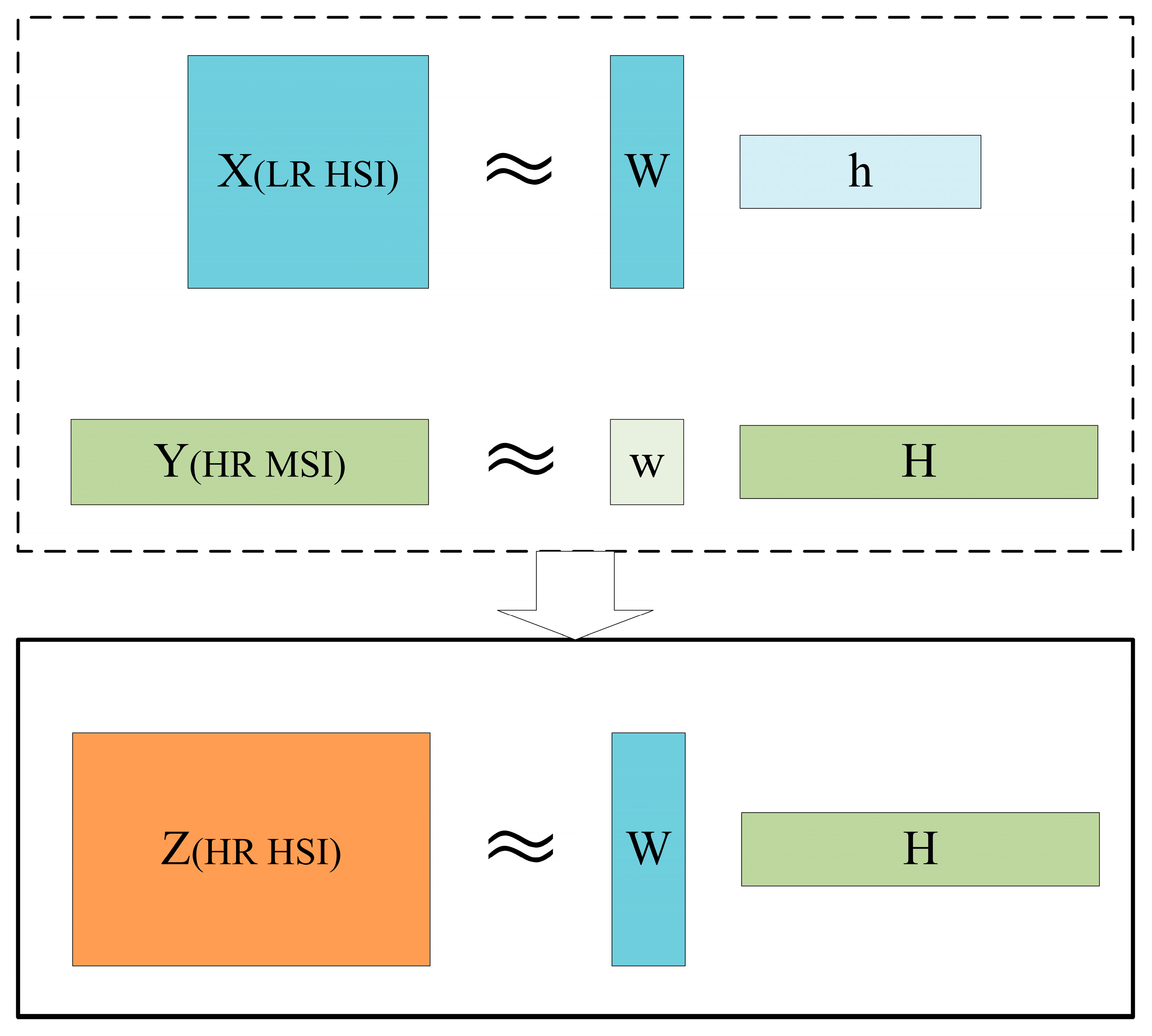
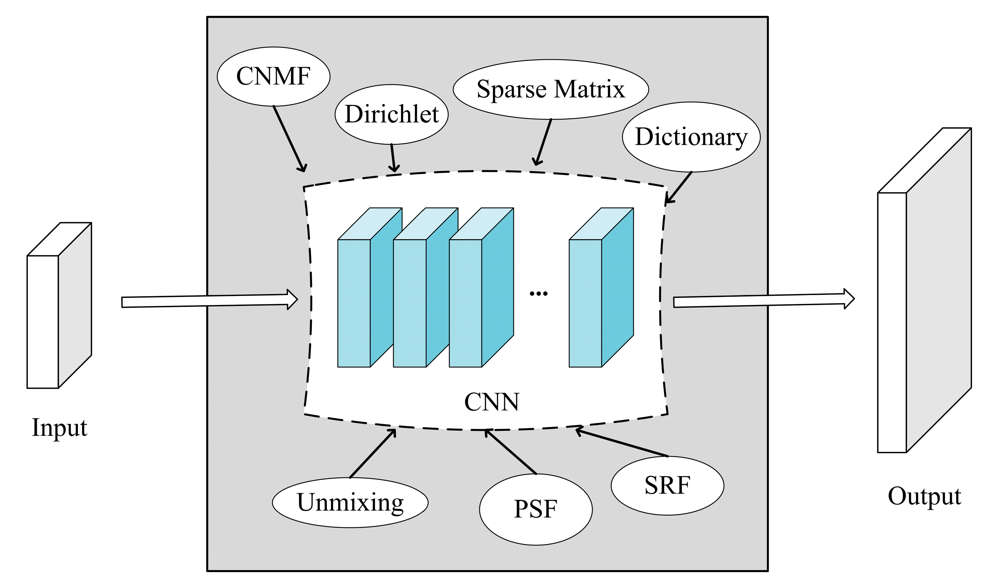
Yokoya, et al. [40] proposed the well-known coupled non-negative matrix factorization (CNMF) algorithm based on a linear spectral mixing model. It reconstructs fused images with high spatial and spectral resolution by fusing low spatial resolution HSI and high spatial resolution MSI with the structure in Figure 2. The hyperspectral and multispectral data are alternately decomposed into an end element matrix and an abundance matrix by the CNMF algorithm, while the sensor observation model is considered in the initialization matrix. Benefiting from its simple update rules, this method is extremely easy to implement. However, the multiple iterations in the unmixing process make the CNMF algorithm very computationally expensive. In 2014, Bendoumi, et al. [41] proposed a new fusion framework. The authors divided the image into multiple sub-images and applied a fusion procedure to each sub-image, which further improved the performance of the proposed SMA-based fusion algorithm.
The existence of plentiful zero elements in a sparse matrix can effectively reduce the computation cost. The meaning of sparse representation is the use of linear combinations of fewer elementary signals to express most or all of the original signals. The elementary signals selected from the overcomplete dictionary are usually called atoms, and any signal has different sparse representations under different groups of atoms [42]. In 2013, the SASFM fusion model proposed by Huang, et al. [43] used sparse matrix decomposition to deal with the remote sensing image fusion problem. In the same year, a non-negative sparse facilitation framework based on RGB image and HSI was proposed [44]. The formulation problem in the form of sparse nonnegative matrix decomposition is handled by alternating optimization, and each subproblem is solved by a convex optimization solver. This method achieves a lower average reconstruction error. In 2014, Akhtar, et al. [45] used LR HSI to learn a dictionary representing the reflectance spectra and then learned sparse coding by the G-SOMP+ algorithm. The sparse encoding was used simultaneously with the spectral dictionary to estimate SR HSI. In 2016, by combining the sparsity and nonlocal similarity of HSIs in the spatial and spectral domains, the algorithm proposed by Li, et al. [46] maintained spectral consistency while producing a large amount of image texture detail and was robust to noise. To exploit the spatial correlation between the learned sparse codes, Dong, et al. [47] proposed an efficient non-negative dictionary learning algorithm using the block coordinate descent optimization technique and a clustering-based structured sparse coding method. The proposed NSSR model performs well in terms of computational efficiency, as well as objective evaluation metrics.
The SR reconstruction method based on SMA, represented by CNMF, is based on a linear mixed spectral model, introduces prior knowledge of the sensor, and successfully works out high-quality fusion data by a simple and intuitive update algorithm. The sparse representation model is established under the condition that an image space is large enough and any image of the same type can be linearly represented by such an image subspace. However, the image space of a class of objects in reality is not linear, which limits the image quality of the HSI reconstructed by the SR method with the introduction of sparse representation theory.
Aside from the above methods, researchers have proposed some other models to solve the HSI SR reconstruction problem [48,49,50,51,52,53]. Akgun, et al. [54] simulated the hyperspectral image acquisition process as a linear deterministic model. Based on this model, the reconstruction problem is set to determine the target image satisfying a linear system of equations. He, et al. [55] focus on the global correlation and local smoothness of the target image by imposing low-rank and total variational regularization on the tensor to generate better-quality reconstructed images. The traditional methods provide a valuable source of inspiration for subsequent researchers by using various mathematical and physical ideas to transform the task of SR reconstruction of HSI into a more understandable mathematical problem. At the same time, traditional methods have problems such as difficult and time-consuming solutions, and inevitably introduce manual errors, which greatly limit the scope of application of traditional methods.

4. Deep-Learning-Based Methods

In recent years, the SR problem for natural images has made great progress, thanks to the increasing popularity of CNNs. Dong, et al. [14] first proposed a CNN-based approach for natural image SR. After that, scholars successively proposed several novel CNN models to improve the natural image SR performance. All these works show that the design of the network architecture is a key factor that affects the image reconstruction effect. However, unlike natural images, HSIs consist of hundreds of spectral bands, and feature extraction for such high-dimensional 3D data is more difficult to work with. Secondly, it is important for HSI SR to ensure the spectral fidelity of the reconstructed images while improving the spatial resolution for better subsequent spectral decoding work. The above reasons predestine HSI SR to be a more difficult task. From the current research status, typically, there are two means of enhancing the spatial resolution of HSI: fusion with other high spatial resolution images, and single image SR. Fusion-based SR techniques can acquire more external prior information, and the reconstructed images usually have finer textures. Single-image-based SR techniques do not require any other auxiliary image, and have better feasibility in practice. From some early models proposed in 2017 to the blossoming of various strategies today, more and more scholars have devoted themselves to the field of hyperspectral SR reconstruction. In this section, we will respectively introduce the basic components, representative works and future directions of DL-based methods.

4.1. Upsampling Frameworks

HSI SR is a typical ill-posed problem. As a key link in the network, the choice of upsampling strategy of the upsampling layer greatly affects the quality of the super-resolved images. At this stage, researchers have proposed a variety of model architectures. Based on the upsampling methods chosen by each model and the position of the upsampling layer within the model, they can basically be grouped into three categories, i.e., front-end upsampling, back-end upsampling, and progressive upsampling.
Front-end Upsampling. Learning the mapping from LR images to HR images directly is not an easy task. In contrast, more researchers prefer to first scale up the LR images and then optimize the scaled-up images using deep neural networks, as shown in Figure 3a. The front-end upsampling strategy was first used in the field of natural image SR. Dong, et al. [14] used bicubic interpolation to first scale the LR image to the desired size and proposed the SRCNN model used to learn the mapping relationship between the interpolated image and the labeled HR image. The 3D-FCNN model for HSI SR proposed by Mei, et al. [18] also utilizes the idea of upsampling at the front end. In general, the most difficult upsampling step is carried out using traditional methods such as bicubic interpolation, and deep neural networks only need to refine these interpolated images to reconstruct high-quality details. This strategy greatly reduces the difficulty of training neural networks, and front-end upsampling has become one of the most mainstream frameworks [56,57]. However, two problems brought by front-end upsampling cannot be ignored. On the one hand, the noise in LR images will be scaled up with the upsampling layer, which leads to undesirable reconstruction results. On the other hand, after scaling up the images, most of the computations are performed in the high-dimensional space, which will bring high computational cost and time cost.
Back-end Upsampling. To reduce the computational cost as well as to fully utilize the learning capability of neural networks, researchers have proposed placing the upsampling operation at the back end of the model to perform it. Specifically, the network carries out the feature extraction process in a low-dimensional space, and sets up a learnable upsampling layer at the back end of the network, as shown in Figure 3b. The upsampling layer usually performs transposed convolution or sub-pixel convolution operations. The FSRCNN [58] model and the ESPCN [59] model are the pioneers of the back-end upsampling strategy, which respectively use transposed convolution and sub-pixel convolution to implement image upsampling. ERCSR [60], as one of the representative works in the field of hyperspectral SR, also uses transposed convolution to perform upsampling operations after the feature extraction process. Since most of the computational processes occur before the upsampling operation, the computational cost is greatly reduced. Therefore, back-end upsampling has also become one of the most popular frameworks among researchers [61,62].
Progressive Upsampling. The back-end upsampling strategy effectively reduces the computational cost of the network, but learning large scaling factors (e.g., 8×) as a one-step upsampling strategy is a difficult task. Therefore, the progressive upsampling strategy was proposed [63]. The progressive framework decomposes a difficult learning task into multiple simple tasks, which greatly reduces the learning difficulty of the network and provides a feasible direction for large-scale SR tasks. Specifically, this strategy sets the upsampling layer in multiple stages of the network so that the image is scaled up after each stage until the desired resolution is reached, as shown in Figure 3c. The SSPSR model proposed by Jiang, et al. [64] first upsamples the grouped sub-images and then performs a secondary upsampling of the complete image made by fusing the interpolated sub-images. This architecture alleviates the difficulty of feature extraction in HSIs and makes the overall training more stable. At the same time, the model with the progressive upsampling strategy has some problems, such as the need for more accurate modeling and the design of complex neural networks for each stage.
With the exception of the above three upsampling strategies, other scholars use iterative up-and-down sampling strategies [65] to solve the SR problem, which effectively explores the deep mapping relationship between LR images and HR images by repeatedly performing upsampling and downsampling operations. Various upsampling strategies have their advantages and disadvantages, and meet different design requirements. As the most essential step of the SR task, it is crucial to select a suitable upsampling strategy for the model.

4.2. Upsampling Methods

In Section 4.1, we introduced three mainstream upsampling frameworks. After determining the upsampling framework, it is also important to decide how to implement the upsampling operation. In previous SR research, scholars have proposed many traditional upsampling methods. However, with the development of DL, end-to-end upsampling methods based on neural networks have gradually become mainstream. This section presents the traditional interpolation-based upsampling methods and the learning-based upsampling methods, separately.

4.2.1. Interpolation-Based Upsampling

Image interpolation, i.e., resizing a digital image according to a predefined scaling factor. The most commonly used interpolation algorithms include nearest-neighbor interpolation, bilinear interpolation, and bicubic interpolation. Because of their simplicity and ease of implementation, interpolation algorithms are widely used in SR models, and are mostly used in front-end upsampling and progressive upsampling structures.
Nearest-neighbor Interpolation. Nearest-neighbor interpolation, by far the simplest interpolation means, requires only the value of the nearest pixel to be selected for each location to be interpolated. The advantages of this interpolation algorithm are that is easy to understand and has a simple algorithm and fast operation speed. However, only the value of the nearest pixel is considered, without the influence of other pixels, which makes the grayscale value of the resampled image discontinuous and the interpolated image often has a significant mosaic effect.
Bilinear Interpolation. Bilinear interpolation, as the name implies, is an algorithm that implements linear interpolation in two directions. Specifically, linear interpolation is first used in one direction of the two-dimensional data, and then another linear interpolation is completed in the other direction. Although the above operation is linear in position as well as pixel values, as a secondary sampling means, the values of the four pixels around the interpolation point can be taken into account, having a larger perceptual field than the nearest neighbor interpolation. Therefore, the bilinear interpolation ensures the simplicity of the algorithm while obtaining a more excellent interpolation effect compared with the nearest-neighbor interpolation. However, although this method considers the grayscale values of the surrounding four pixels, it does not consider the effect of the rate of change of grayscale values between neighboring pixels, so that the high-frequency information of the interpolated image is damaged, and blurred image edges are often obtained.
Bicubic Interpolation. Bicubic interpolation has become the most widely used interpolation algorithm in SR, by performing cubic interpolations in two directions. While the pixel values of the interpolation points of bilinear interpolation are obtained by weighting the four surrounding pixels, bicubic interpolation is obtained by weighting the sixteen nearest pixels, and the weight occupied by each pixel is determined by the distance from that pixel to the interpolation point. Bicubic interpolation takes into account the effect of the gray value of the four nearest pixels, while also taking into account the effect of the rate of change of the surrounding gray values, thus obtaining smoother edges, fewer artifacts, and less lost-image information than the previous two interpolation methods. However, the higher computational accuracy is obtained along with a larger computational effort.
In addition to the above three commonly used interpolation algorithms, researchers have also proposed interpolation algorithms such as Sinc, as well as Lanczos. The three interpolation algorithms all possess strong interpretability, which is the advantage of traditional algorithms. However, the upsampling method based on interpolation can only obtain and utilize the information of the image itself, and cannot bring information outside the image. Most of the time it also brings bad effects, such as high computational effort and noise amplification. Therefore, more and more scholars are exploring the use of learnable upsampling layers to implement image upsampling.

4.2.2. Learning-Based Upsampling

Since the traditional interpolation-based upsampling method cannot introduce external prior information and is not applicable as an upsampling layer in the back-end upsampling structure, scholars have introduced learning-based upsampling layers into SR research. Transposed convolution as well as pixel shuffle are respectively introduced in this section.
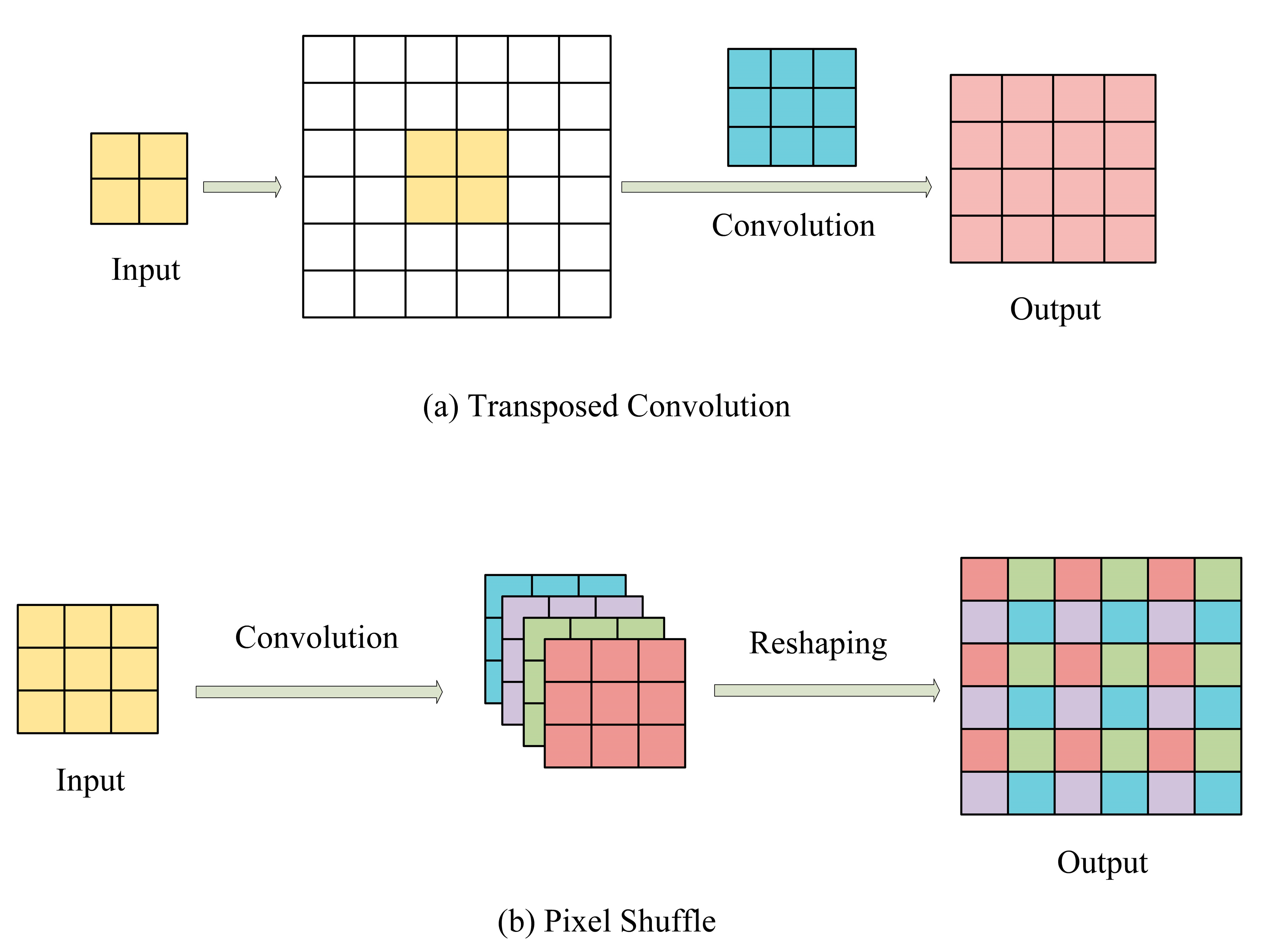
Transposed Convolution. Transposed convolution, also known as deconvolution, was first applied to solve the SR task in the FSRCNN [58] model. It is worth noting that transposed convolution is not the inverse operation of regular convolution, but exists as a special type of convolution. Specifically, transposed convolution first increases the size of the input image by zero padding, and then performs the convolution operation on the padded image to achieve the purpose of increasing the image resolution. As shown in Figure 4a, suppose the input image is a 2 × 2 size, and we want to use a 3 × 3 size convolution kernel to change the image resolution to twice the original one, i.e., to obtain a 4 × 4 size output image. First, we zero-fill the original image to make it 6 × 6 , and then use the 3 × 3 convolution kernel to perform convolution on the 6 × 6 image to obtain a 4 × 4 output, which completes the process of twice upsampling. The above example is with s t r i d e = 1 and p a d d i n g = 0 . Other parameters can be set to achieve different padding and magnification. Transposed convolution makes the upsampling process more flexible by continuously refining the image magnification operation in a learnable way. Transposed convolution is also the most popular upsampling method among the back-end upsampling structures.
Pixel Shuffle. Pixel shuffle, also known as sub-pixel convolution, is another way of upsampling LR images, and was first applied to solve the SR task in the ESPCN [59] model. SSPSR [64] and HSRnet [66] models are its representative works in the field of HSI SR. Pixel shuffle is a sub-pixel image-based convolution algorithm. When the convolution operation is performed on a sub-pixel image obtained by zero padding, the kernel is effectively convolved with the non-zero pixels in the sub-pixel image. The weights corresponding to their space in the kernel are activated, while the weights corresponding to the sub-pixels are not calculated. Different parts of the filter take turns to participate in the convolution calculation when sliding over the sub-pixel image. The output obtained is the same size as the sub-pixel image. Since the activation of the weights in the convolution kernel is independent, the shape of the kernel can be changed according to the batch of activated weights, to accomplish the above operation. Specifically, pixel shuffle first increases the number of feature map channels by convolution, and then rearranges the pixels of all channels to achieve image upsampling. As shown in Figure 4b, suppose we need to r -fold the input of size w × h × C to finally obtain an output image of size r w × r h × C . The pixel shuffle method first obtains a feature map of size w × h × r 2 C by convolution, and then periodically shuffles the pixels on this feature map to arrange them into an output image of size r w × r h × C . Pixel shuffle uses a unique way of extracting features to solve the upsampling problem, providing more possibilities and inspiration for constructing high-performance networks.
There is no absolute advantage or disadvantage to any of these upsampling methods, including interpolation-based and learning-based upsampling methods. The adaptation to other components of the network needs to be considered before choosing an upsampling method. It is crucial for researchers to choose the suitable upsampling method for their networks.

4.3. Network Design

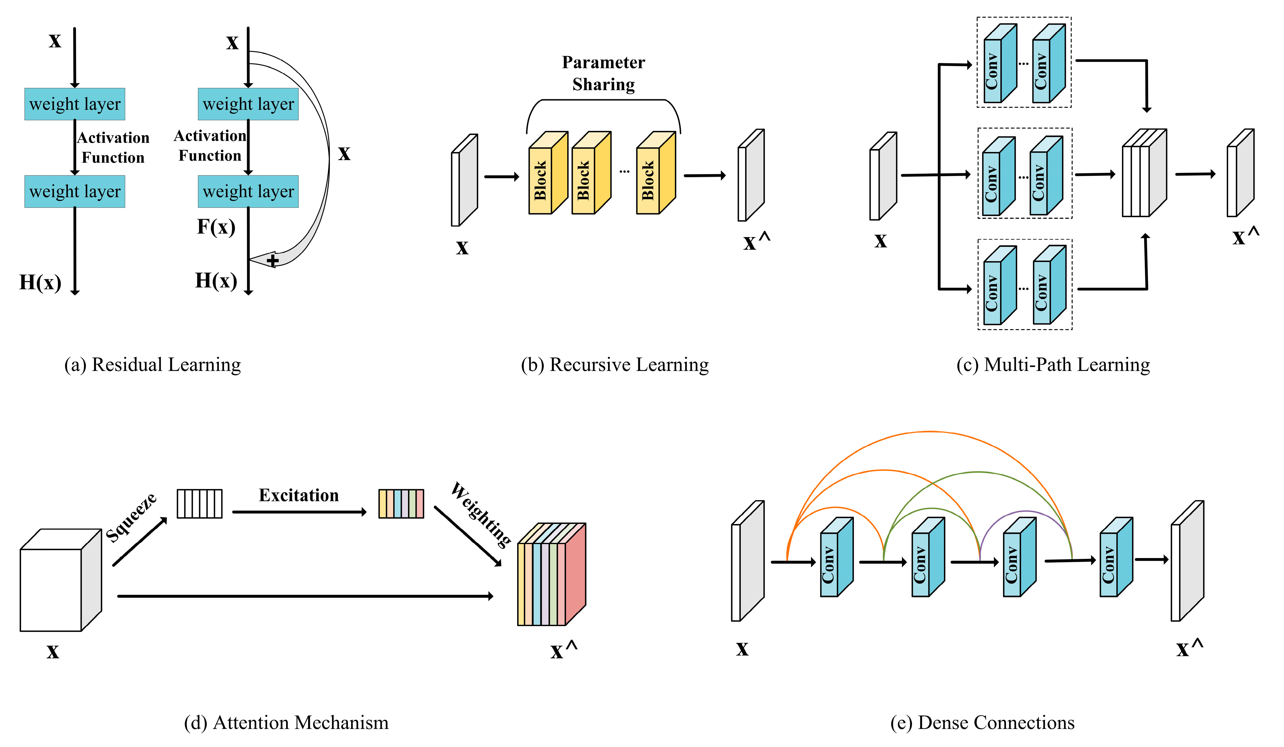
It has become a consensus in the field of deep learning that network design can significantly impact the capabilities of a model. In the field of HSI SR, researchers have employed various network design strategies to build complete networks based on the three upsampling frameworks described above. In this section, we introduce each of the commonly used network structures and analyze their advantages and limitations. The structures of these networks are shown in Figure 5.
Residual Learning. For deep network models, depth is a very important factor that affects the ability of the model, and residual learning [67] is thus born. Deep neural networks naturally integrate features at different levels of low, medium and high, and the level of features can be enriched by deepening the network. Therefore, when building models, researchers tend to use deeper network structures in order to extract higher-level features. However, as the number of operation layers increases, the network will produce a degradation phenomenon, that is, when the model capacity tends to saturate; as long as the network still has depth and either forward or backward propagation, there must be more or less information loss or decay. When a feature map loses some of its useful information, then the performance of the network will degrade. Assuming that a researcher designs a network where an optimal number of layers exists, often the deep network is designed with redundant layers, and the ideal state is that these redundant layers can complete a constant mapping, i.e., the output through the redundant layers is guaranteed to be exactly the same as the input.
As in Figure 5a, assuming that the layer is redundant, for the first conventional structure, the parameters learned by the layer need to be able to satisfy H x = x to complete the constant mapping. For the second residual learning structure, it needs to satisfy H x = x + F x , when only F x = 0 needs to be learned. Learning F x = 0 is much simpler than learning H x = x . The proposed residual learning effectively alleviates the problem of model degradation and gradient vanishing, making deep neural networks go deeper, in a real sense. Subsequent hyperspectral SR works are almost inseparable from the residual learning structure.
Recursive Learning. In order to learn more high-ranking features without introducing overwhelming parameters, scholars have introduced recursive learning (applying the same module multiple times in a recursive manner) into the SR domain, with the structure shown in Figure 5b. From DRCN [68] to CARN [69] to SRFBN [70], recursive learning ideas have been developed massively in natural image SR tasks. In the field of hyperspectral SR, GDRRN [56] uses a single residual unit as the recursive unit for nine recursions, where all residual units share the same weight, greatly reducing the number of model parameters. In general, recursive learning does allow learning more high-ranking representations with relatively fewer parameters, but still does not avoid the high computational cost. Additionally, recursive learning inherently introduces the problem of gradient vanishing or gradient exploding, so it is a wise choice to combine residual learning with recursive learning.
Multi-Path Learning. Multi-path learning refers to assigning images or features to multiple paths to perform the same or different operations, and fusing them back for better modeling capability, as shown in Figure 5c. SSPSR divides an HSI into multiple groups from spectral dimensions, and then fuses the features extracted from each group after each group passes through different paths with shared weights. Compared with SSPSR, the neighboring-group integration module is proposed in the GELIN [71] model to enhance the complementary information among image subsets, effectively supplementing the missing details. Inspired by the spectral difference network SDCNN [72], Hu, et al. [73] proposed feeding two adjacent bands and the difference feature maps between them into three network branches separately, to better exploit the spectral correlation between adjacent bands. In addition, the Interactformer [74] model consists of a transformer structure and a 3D convolutional network, where the two parallel branches are used to capture global and local features, respectively, and interactive connections are used to enhance the information fusion between the branches. For the high dimensionality and complexity of hyperspectral data, multi-path learning is a promising research direction.
Attention Mechanism. Each image element of a hyperspectral image can be regarded as a high-dimensional vector, reflecting the spectral characteristics of the object corresponding to that image element, so there is a strong dependence and correlation between channels. Hu, et al. [75] used the “Squeeze-and-Excitation” module to add an attention mechanism to the channel dimension with the structure shown in Figure 5d. Specifically, a small network is used to automatically learn the importance of each channel, and then assign a weight to each feature based on this importance, so that the network focuses on certain feature channels. RCAN [76] combines the channel attention with the SR task, which greatly improves the SR performance of the model. To mitigate the spectral distortion of reconstructed images, Li, et al. [77] proposed combining the band attention mechanism with 3D convolution to fully exploit the spectral information. Zheng, et al. [78] firstly applied the spatial–spectral attention mechanism to the HSI panchromatic sharpening task in order for the network to learn spatial and spectral information adaptively. SGARDN [79] is also the representative work for refining the reconstructed image details by using the attention mechanism. Due to the special need for spectral fidelity in this research area, the attention mechanism is gradually becoming an indispensable part of network construction.
Dense Connections. Similar to residual learning, dense connections also realize the direct correlation between the previous layer and the subsequent layer through skip connection, but this connection includes the connection between the current layer and all layers, which is the reason for its “dense” structure, as shown in Figure 5e. Obviously, the most important feature of dense connections is the ability to reuse features including low-level features and high-level features, which is a superior aspect compared with ordinary skip connections. Since DenseNet [80] was proposed, more and more scholars have been solving SR problems based on dense connections [81,82]. Due to the structural characteristics of dense connections, they inevitably cause structural redundancy while enhancing information dissemination. To alleviate this problem, Dong, et al. [83] used a cross-feedback strategy based on dense connections to achieve more efficient and hierarchical signal transmission. How to achieve more efficient feature reuse is probably the most important issue to be explored when using dense connections.
With the continuous deepening of the study of neural networks, more and more forms of networks are being developed and applied. Apart from the above five types of networks, common structures such as group convolution [84] are also available. With the gradual diversification of network designs, the performance of SR models is also improving. Exploring network structures that are more suitable for SR tasks has become one of the hottest topics in the field.

4.4. Loss Functions

In the field of deep learning, the loss function often represents the learning objective of a deep network. The loss function for SR tasks can embody the reconstruction error and constrain the optimization process of the model. Next, we provide a brief introduction to several loss functions commonly used in the HSI SR field.
Pixel-wise Loss. L1 and L2 loss are representatives of pixel-wise loss. Both of them directly calculate the pixel-wise error for the labeled HR image and the reconstructed SR image, and the difference lies in the different calculation methods used to calculate the difference of the corresponding pixels; the expressions are given in Equations (16) and (17), respectively:
L l 1 I ^ , I = 1 H W C i , j , k I ^ i , j , k I i , j , k
L l 2 I ^ , I = 1 H W C i , j , k I ^ i , j , k I i , j , k 2 .
The former calculates the MAE, while the latter obtains the MSE. Compared with L1 loss, L2 loss can powerfully handle larger errors, but cannot make an effective penalty for smaller errors, thus often leading to over-smoothing of results. This makes the L1 loss the better option in most cases. Besides the above two losses, other scholars have used a loss function called Charbonnier loss [63,85] with the following expression:
L C h a I ^ , I = 1 H W C i , j , k I ^ i , j , k I i , j , k 2 + ε 2 ,
where ε is the stability constant. Considering that the definition of PSNR has a high correlation with MSE, and PSNR reaches its maximum value when pixel-wise loss is minimized, pixel-wise loss is the loss function most favored by researchers. However, the reconstructed images generated by pixel-wise loss guidance often lose high-frequency details and produce overly smooth textures, which cannot achieve excellent results in visual perception.
Adversarial Loss. Generative adversarial networks (GAN) [86] were pioneeringly proposed in 2014. As a network architecture with unique advantages for generative tasks, more and more scholars have successfully introduced generative adversarial ideas into the study of image SR, among which SRGAN [87] is a representative work of GAN in the field of natural image SR. Specifically, GAN consists of a generator responsible for generative tasks and a discriminator responsible for identifying whether the output of the generator obeys the target distribution. When training the GAN network, the generator and discriminator need to be trained alternately. When training the discriminator, the generator needs to be fixed in order to improve the discriminative ability of the discriminator; when training the generator, the discriminator needs to be fixed in order to generate results that can fool the discriminator. By alternating the above training process, after sufficient adversarial training the generator is able to generate results that are consistent with the target distribution, while the discriminator is unable to distinguish the source of the input data. When applied to the SR domain, the generator plays the role of the SR model and the discriminator is used to identify whether the input image is the reconstructed image from the generator or labeled image. Ledig, et al. [87] proposed the adversarial loss as follows:
L G A N G I ^ ; D = log D I ^
L G A N D I ^ , I ; D = log D I log 1 D I ^
where L G A N G and L G A N D represent the adversarial loss of the generator and discriminator, respectively. In extensive mean opinion score tests, it was found that the model trained using the adversarial loss obtained a lower PSNR compared with the pixel-wise loss, but the reconstructed image exhibited better visual perception [88]. The reason for this is that the discriminator is able to extract a portion of the underlying patterns in the labeled HR images and use this to guide the generator to reconstruct a more realistic result.
Total Variance Loss. When performing the SR task, how to suppress the noise in the reconstructed image is a problem worth exploring. Aly and Dubois [89] first used the total variance loss to solve the SR problem, and Li, et al. [77] combined the total variance loss with other losses to constrain the reconstructed HSI. The total variance is calculated as the difference between each pixel and its immediate neighbors in the horizontal and vertical directions, and is usually defined as follows:
L T V I ^ = 1 H W C i , j , k I ^ i , j + 1 , k I ^ i , j , k 2 + I ^ i + 1 , j , k I ^ i , j , k 2 .
A noise-contaminated image has a larger total variance compared with a noise-free image, so the process of minimizing the total variance is the process of limiting the noise.
Perceptual Loss. To evaluate the reconstruction quality at a deeper level, Johnson, et al. [90] introduced perceptual loss into the SR domain. The idea of perceptual loss is to measure the perceptual quality of the reconstructed image by comparing the high-level semantic differences between the reconstructed image I ^ and the labeled image I . Specifically, the reconstructed image and the labeled image are fed as inputs to a pre-trained classification or detection network (usually VGG [91] or ResNet [67]), and the “high-level representations” extracted at the l -th layer of the network can be denoted as φ l I ^ and φ l I , respectively. The perceptual loss is expressed as the Euclidean distance between the two, as follows:
L P e r c e p t u a l I ^ , I = 1 H l W l C l i , j , k φ i , j , k l I ^ φ i , j , k l I 2 .
While pixel-wise loss requires an exact match between the point-to-point pixel values of the reconstructed image and the labeled image, perceptual loss constrains the former to be close to the latter in terms of perceptual quality, and thus is more likely to produce reconstructed results that match visual perception, and is widely used in the field of SR.
Cycle Consistency Loss. The style transfer network CycleGAN proposed by Zhu, et al. [92] provides a new idea for unsupervised SR. Later, Yuan, et al. [93] proposed the well-known CinCGAN, which uses an embedded loop structure to complete the “denoising-SR” process. The cycle consistency loss is the key for the above model to work. Specifically, the HR image I ^ reconstructed by the generator network needs to be fed into the degradation network again for a LR image I ^   l r with the same size as the input image I l r . The cycle consistency loss requires that the I ^   l r obtained by the degradation network has the same pixel-wise performance as the initial LR image I l r , i.e.,
L C y c l e I ^   l r , I l r = 1 H W C i , j , k I ^ l r , i , j , k I l r , i , j , l 2 .
By comparing the pixel-wise loss of two LR images, the optimization process of the model is not dependent on the HR labeled images for the purpose of unsupervised SR. Most subsequent SR models based on CycleGAN are inseparable from the constraint of cycle consistency loss. With the increasing popularity of unsupervised learning, the cycle consistency loss has inevitably become one of the most widely used loss functions in this field.
The more comprehensive the consideration in constructing the loss function, the more accurate its constraints on the network. Therefore, in reality, based on different network characteristics and purposes, the loss function chosen by scholars is usually a combination of multiple single losses. In addition to the above commonly used loss functions, many scholars incorporate SAM restrictions into the construction of the loss function [71] in order to better constrain the reconstruction of spectral information.

4.5. Representative Works with Different Strategies

Before introducing the DL-based SR reconstruction techniques for HSIs, we briefly review the development process of natural image SR techniques. Before the emergence of DL-based algorithms, reconstruction-based methods were the mainstream techniques for image SR, including iterative back projection method [94], KK [95], total-variation regularization method [89], and deconvolution method [96], etc. In 2014, Dong, et al. [14] first introduced convolutional neural networks into the field of image SR and constructed the SRCNN model with a relatively simple structure. Based on this, FSRCNN [58] and ESPCN [59] introduced two different learning-based upsampling methods. To build deeper networks, Kim, et al. [97] first used residual learning in an SR network, which increased the perceptual field while speeding up the convergence, and VDSR was the first deep network model in this field. DRCN [68] and DRRN [98] are both representative works based on recursive learning which greatly reduced the number of parameters by sharing parameters. Lai, et al. [63] proposed a pyramidal network structure. The progressive upsampling strategy proposed by this model can still achieve good reconstruction results in the face of large scaling factors. Ledig, et al. [87] introduced GAN to the field of image SR for better model generalization. In addition, SRFeat [99] and ESRGAN [100] are also excellent works based on GAN. CinCGAN [93] realizes unsupervised SR by cycle consistency loss, and most of the subsequent related researches are based on this model. KernelGAN [101] learned the parameters of fuzzy kernel through the cross-scale similarity to better mine the internal prior information. Based on the above representative works, the field of natural image SR has entered a boom period [70,102].
From the germination of deep-learning-based hyperspectral SR reconstruction techniques in 2017 to the various network models being proposed today, scholars have been striving to find a more suitable SR method for HSI. Since hyperspectral data has hundreds of channels in the spectral dimension, this 3D characteristic predestines the fact that the hyperspectral SR task cannot be solved by the same method for the natural image. The works in recent years can be divided into two main technical lines, which are single-image-based methods and fusion-based methods. The method based on single image can only obtain relatively limited external prior information, so scholars prefer the fusion-based approach at this stage. The fusion-based methods usually have both MSI and panchromatic image (PAN) in the choice of auxiliary images. MSI usually has similar properties to his, while carrying part of the spectral information. Palsson, et al. [103] proposed solving the HSI-MSI fusion problem using a 3D convolution-based network as early as 2017 and reducing the dimension of HSI by PCA before performing the fusion operation, to cut down the computational cost. Yang, et al. [104] designed a two-branch network to extract the spectral information of each pixel in the HSI and the spatial information of its spatial neighborhood in the MSI, and then fused the two extracted features efficiently through a fully connected layer. Xu, et al. [105] realized information fusion with MSI at multiple scales by gradually amplifying HSI. The UAL framework designed by Zhang, et al. [57] uses a two-stage network in which the LR image is first passed through a generalized fusion module and then fed into an adaptive module for a specific data distribution, to obtain more refined texture features. Dian, et al. [106] achieved SOTA fusion results based on subspace representation and using CNN, which is used for grayscale graph denoising, to regularize the estimation of coefficients. Zhang, et al. [107] realized blind HSI SR by jointly training a generator network and two degradation networks based on deep image prior. Xie, et al. [108] proposed a blind MHF-Net model that can cope with the case of mismatch between training and testing data which greatly improves the practicality and application value of this technique. The process of obtaining HR HSI by fusing LR HSI with HR PAN of the same scene is often referred to as HS pansharpening. Zheng, et al. [78] utilized deep hyperspectral prior and used the channel–spatial attention mechanism for the first time for pansharpening, which effectively preserved the spectral information. The MSSL model proposed by Qu, et al. [109] unsampled and downsampled the HSI and PAN, respectively, extracted features from images at different scales through a multipath network, and finally fused the spatial and spectral features from different scales. This process uses multiple shallow networks to extract spatial–spectral features, which greatly reduces the computational cost. Guan and Lam [110,111] took HR, PAN and the cascade of the two as the input of a three-branch network, separately, and fused the feature information extracted from each branch at different stages through a multi-level attention module, which effectively enhanced the information interaction between images. Zhuo, et al. [112] used five high-pass filters, a deep–shallow fusion network, and spectral attention mechanism to fully exploit spatial information and spectral features. Dong, et al. [113] proposed an image segmentation-based injection gain estimation algorithm, which can effectively alleviate the oversharpening problem. In addition, CFDcagaNet [83] is also an excellent work for pansharpening.
Despite the numerous difficulties encountered during research, researchers never give up the pursuit of faster speed and better results. In the previous four subsections, we introduced each component of the SR model, interspersing some classical networks. In this section, we present a systematic introduction of some of the most representative models to date, at a more macro level. Based on the extensive literature research and summary analysis, we find that DL-based HSI SR works basically start from three strategies, namely, key bands, based on traditional framework, and 2D/3D convolution. To discuss the 2D/3D convolution strategy more effectively, we designed two sets of comparative experiments and analyzed the experimental results. Finally, we summarize the structural features of some of the representative HSI SR models in a tabular layout. This section is also the central part of this review.

4.5.1. Key Bands

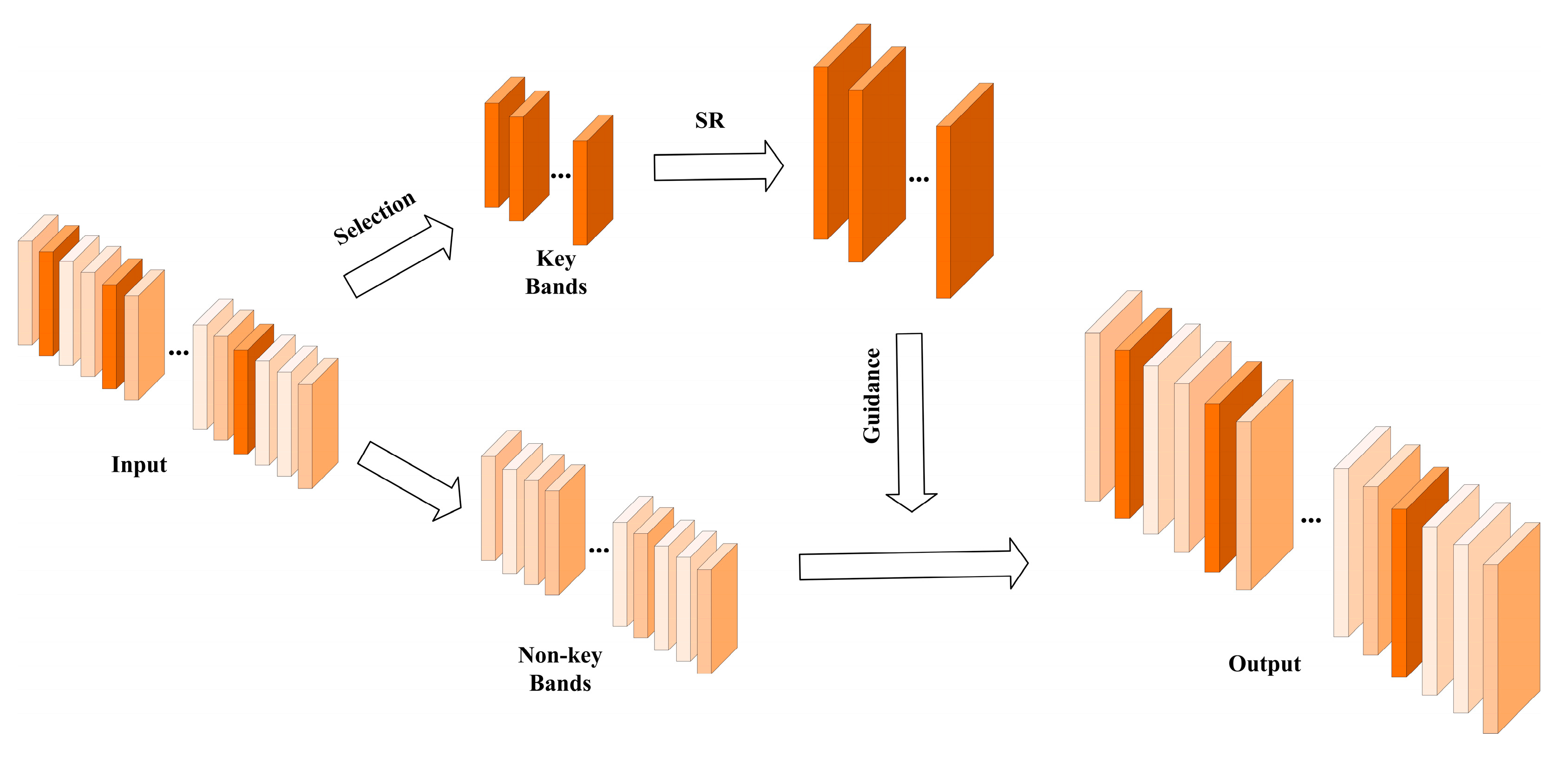
Hyperspectral sensors usually collect the reflection information of objects in hundreds of consecutive narrow bands over a certain electromagnetic spectrum, and HSIs have more spectral information compared with natural images. First, compared with single-channel panchromatic images and three-channel RGB images, feeding a complete HSI with hundreds of spectral dimensional channels as input to an SR reconstruction network will bring great computational cost and model training difficulty. Second, during the imaging process, the collected information is inevitably corrupted by noise, and this corruption is different among different bands. The information from different channels is a description of the same scene in different bands, but the quality may vary with the band, so those bands with good information quality have a higher reference. Thus, the researchers propose the strategy of SR reconstruction utilizing key bands, as shown in Figure 6.
SEC_SDCNN [72] uses the PCA method to select the key bands. The PCA method ensures that most of the information is retained in a small number of significant principal components and that the principal component images contain rich spatial information. Therefore, the authors use the first principal component image as a reference to select the key bands, i.e., the band with the highest similarity to the first principal component image (using multiple grayscale co-occurrence matrix for image texture measurement). In order to complete the unabridged HSI SR task, the model attempts to reconstruct the key bands with super resolution first, and then extend from the magnified key bands to the non-key bands. DFMF [114] divides the complete set of bands into several highly correlated subsets, and then selects the band with the highest entropy in each subset as the key band of that subset, according to the information theory. An MSI with high spatial resolution is obtained by reconstructing the key bands, and then the original HSI with low spatial resolution and the high spatial resolution MSI are fused utilizing the classical CNMF algorithm, to obtain a high spatial resolution HSI. Different from the above, the BDCF model proposed by Sun, et al. [115] divides both LR HSI and HR MSI used for fusion into overlapping and non-overlapping parts from the spectral dimension. The overlapping bands of the two are first used to fuse the high-quality HR data, and then the mapping relationship between the overlapping and non-overlapping parts of the LR HSI is learned by a neural network. Finally, this mapping relationship is applied to the HR data of the overlapping part fused in the first step to obtain the HR data of the non-overlapping part, and the HR HSI is then merged from these two parts of the HR data.

4.5.2. Based on Traditional Framework

Compared with DL-based SR techniques, traditional SR algorithms do not require training of the model, but at the cost of lower accuracy. Apart from the DL-based hyperspectral SR approach, which learns the mapping from LR HSI to HR HSI in an end-to-end manner, some scholars proposed using a neural network as an auxiliary tool to better use the framework or ideas of traditional methods to solve SR problems, as shown in Figure 7.
TLCNN [116] borrows the transfer learning idea to apply the pre-trained CNN model on the natural image dataset to LR HSI band by band to obtain HR HSI, and then enhance the collaboration between HR-LR HSI pairs using a collaborative non-negative matrix factorization algorithm, thus requiring the final estimated HR HSI to have same end elements as LR HSI. This method transfers the mapping relationship between LR-HR image pairs from natural images to hyperspectral images, providing the possibility of interoperability between the two domains. The uSDN [117] uses an “encoder–decoder” structure to implement HSI SR. The neural network is used to respectively resolve the end element matrix and the abundance matrix from the LR HSI and HR MSI, and the Dirichlet distribution is used to constrain the abundance matrix. The process of solving end-member matrix and abundance matrix is transformed into a deep network learning process which enhances the generalization of the model. Zheng, et al. [118] proposed using an autoencoder structure to solve the pixel unmixing problem and to enhance the interaction between abundance matrices by a learnable PSF. There are many other works such as MHF-net [119], URSR [120], MIAE [121], and GJTD-LR [122]. Although DL-based SR techniques have become mainstream, the ideas provided by traditional methods still have a profound influence on the research in this field.

4.5.3. 2D/3D Convolution

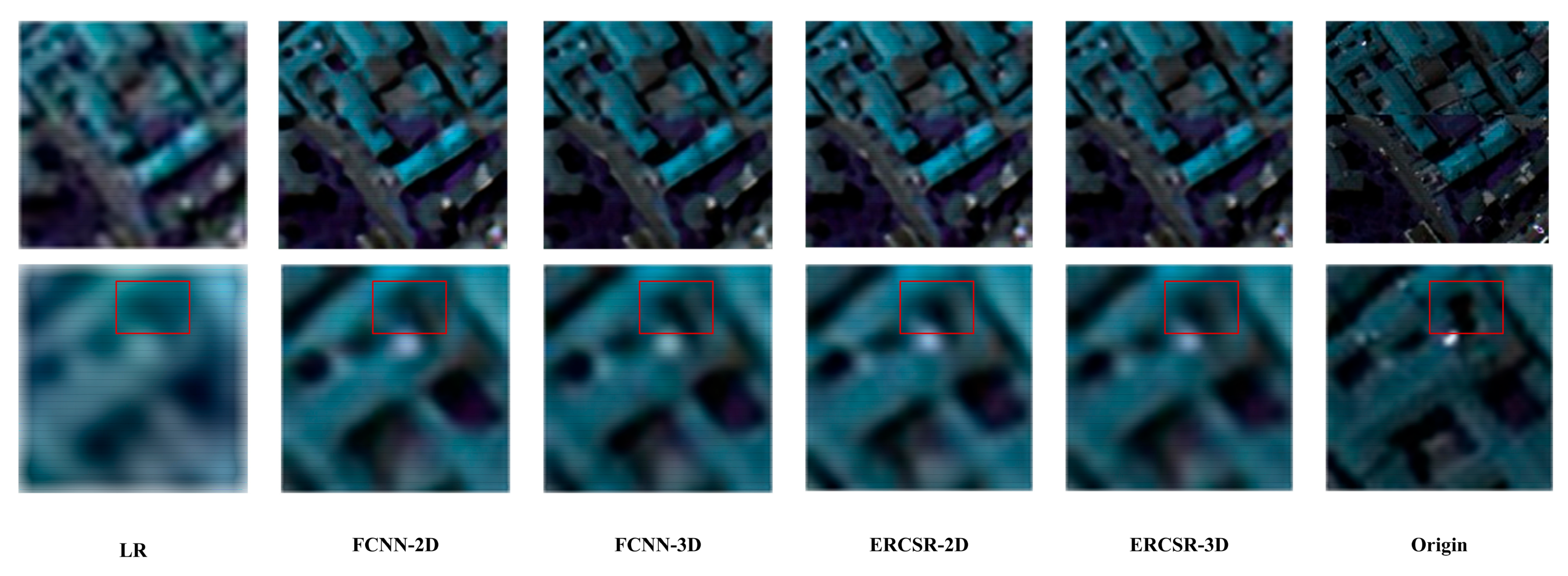
Compared with natural images, the greatest value of HSI lies in the ability to collect the spectral signal of the observed target, which is also the core of supporting the later image interpretation work. Therefore, for the task of SR reconstruction of HSI, it is one of the core requirements for SR models to reduce spectral distortion and improve the spectral fidelity of reconstructed images while improving spatial resolution. Some scholars believe that, compared with the most commonly used 2D convolution, 3D convolution can better capture the information of spectral correlation and is more in line with the 3D characteristics of hyperspectral data. 3D-FCNN [18] first proposed using 3D convolution to explore spatial information and spectral correlation, and HSRGAN [61] first applied the GAN using 3D convolution to the hyperspectral image SR. Both of the above methods use regular 3D convolution. However, 3D convolution brings an additional number of parameters and great computational cost while exploring spectral correlation. Considering this, researchers have modified the convolution kernel k × k × k to k × 1 × 1 and 1 × k × k , with typical algorithms such as MCNet [62], by which the network parameters are greatly reduced and allow for a more in-depth design of the network. Nevertheless, its use of parallel structures to extract features leads to modular redundancy. ERCSR [60] alternately uses 2D and 3D units to relieve the structural redundancy problem, which enhances the learning capability of the model in spatial domain by sharing spatial information. Importantly, it reduces the size of the model while improving network performance, compared with networks using only 3D convolution. Additionally, the use of the SAEC module allows the exploration of the spectral and spatial information in horizontal or vertical directions, in parallel. In order to make better use of the similarity between bands, Wang, et al. [123] proposed a two-branch network, in which the 2D network branch and the 3D network branch focus on mining spatial information and spectral correlation, respectively.
In this section, we will discuss the advantages and shortcomings of 2D convolution and 3D convolution in solving the HSI SR problem, design two sets of related comparative experiments based on the CAVE dataset and Pavia Centre dataset, and analyze and summarize the experimental results.

Mechanisms

First, we observe the difference between performing multi-channel 2D convolution and 3D convolution on the HSI. Suppose for an image of size 5 × 5 × 5 the spatial dimension of the convolution kernel is chosen to be 3 × 3 , the result of convolution is a single-channel map, and the convolution operation is performed by default without padding and in steps of one. As shown in Figure 8, when performing multi-channel 2D convolution, the size of the convolution kernel is 3 × 3 . The number of parameters and multiplication operations performed are 45 and 405. When performing 3D convolution, the number of parameters and multiplication operations are 27 and 729, while the size of the kernel is 3 × 3 × 3 . The reason for this is that the depth of the convolution kernel does not need to match the channel dimension of the input data when performing 3D convolution, which results in fewer parameters. At the same time, the reduced depth of the convolution kernel brings the sliding in the spectral dimension, which is not needed during 2D convolution. Excluding the case of excessive step size, in general the sliding causes the input data to be used more times, which makes it more computationally expensive to use 3D convolution. Of more concern is that the single-channel output obtained by 3D convolution is a data cube, which triggers an explosion of computation in subsequent convolution operations.

Experiments and Results

In order to compare the advantages and disadvantages of 2D convolution and 3D convolution from different perspectives, we designed two sets of comparative experiments. The performance differences between 2D convolution and 3D convolution are compared and analyzed from four perspectives: the time consumed by each epoch during training, and three objective image evaluation metrics (PSNR, SSIM, and SAM).
Part A
Firstly, the selection and design of models are introduced. For comparing the performance of 2D convolution and 3D convolution in a more reasonable and feasible way, we choose the three most classical models in the field of SR as benchmark models, namely SRCNN [14], FSRCNN [58] and ESPCN [59]. Among them, SRCNN adopts a front-end upsampling structure, and the upsampling method is bicubic interpolation, while FSRCNN and ESPCN both adopt a back-end upsampling structure; the upsampling methods are transposed convolution and pixel shuffle, respectively. Since all three models are research results for natural images, we adjust the hyperparameters in the models to be more suitable for processing HSIs including the number of output channels per layer and the size of the convolution kernel. Specifically, based on the original model, the 2D version of the new model adjusts the hyperparameters, and the 3D version of the new model replaces all the 2D convolutions in the initial model with 3D convolutions. In the experiments, it was found that the performance of the 2D version of the ESPCN model was far from that of the 3D version. To further explore the reasons, two additional 3D versions of the model were added, specifically by extending the original three convolutional layers to eight and twelve layers. In summary, eight models are designed, namely SRCNN-2D, SRCNN-3D, FSRCNN-2D, FSRCNN-3D, ESPCN-2D, ESPCN-3D1, ESPCN-3D2, ESPCN-3D3; 2 × , 3 × , and 4 × SR are performed on the images, and the performance differences are compared from several perspectives.
Secondly, the dataset used in the experiment is introduced. The CAVE dataset we selected for this experiment contains 32 images, each with a spatial resolution of 512 × 512 , 31 bands, and an imaging wavelength range of 400–700 nm in steps of 10 nm. The images mainly include Stuff, Skin and Hair, Paints, Food and Drinks, Real and Fake. Due to the small number of images in the CAVE dataset, we randomly selected 24 patches on each image to increase the data for training, and each patch was horizontally flipped, rotated at different angles, and scaled at different magnifications. These patches were downsampled into LR HSI of size 32 × 32 × 31 according to different scale factors, by bicubic interpolation, which is used as the input to the network.
Finally, the experimental details are introduced. For fairness, all training and testing for this experiment were performed in the same environment. The hardware conditions include two Nvidia RTX3090 GPUs, and the batch size of each graphics card is set to 2. All training procedures in this experiment are performed using the Adam optimizer. Because of the large number of models, more adapted hyperparameter settings needed to be chosen for each model in order to more reasonably compare the performance of each model, and it is not possible to strictly unify the experimental settings. Specifically, in the training process, the batch size was set to 16 or 32, and the initial learning rate was set to 0.0001 or 0.00005 or 0.00001.
Table 2 shows all the experimental results and Figure 9 presents the convergence of each model for the 3× SR during training. It can be observed that the time used for each epoch increases substantially for the 3D version of the model compared with the 2D version when trained. This phenomenon is consistent with the mechanism.
Among the three objective evaluation metrics, the PSNR of the images reconstructed by the 3D version of the model is slightly lower than that of the 2D version, but the SAM is significantly superior, and the SSIM is not much different. Specifically, in the SRCNN model comparison, the PSNR values for the 2D model were 0.128 dB, 0.551 dB, and 0.5 dB ahead of the 3D model for the experiments with scaling factors of 2, 3, and 4, respectively, and the SAM values of the 3D model were 0.436, 0.237, and 0.217 lower than those of the 2D model. In the model comparison of FSRCNN, the PSNR values of the 2D model were 0.522 dB, 0.528 dB and 0.637 dB ahead of the 3D model with scaling factors of 2, 3 and 4, respectively, and the SAM values of the 3D model were reduced by 0.475, 0.386 and 0.063, compared with the 2D model. This is due to the fact that the 3D convolution brings about the sliding of the convolution kernel in the spectral dimension. This sliding enhances the continuity of the spectrum and the correlation between different bands, which is a unique advantage of 3D convolution that has been noticed by many scholars. The prerequisite for improving the spatial resolution must be to preserve the original spectral information of the pixels as much as possible, which is one of the core tasks of SR for HSI. The HSI that lose the original spectral information almost lose their value of existence.
In the comparison of the 2D and 3D models of ESPCN, we found that the PSNR, SSIM and SAM values were much worse than those of the 2D model when using the 3D model with the same depth (i.e., ESPCN-3D1). Therefore, we increased the number of convolutional layers to eight and twelve (i.e., ESPCN-3D2 and ESPCN-3D3). As the number of layers increased, the performance of the model gradually became better, but still differed significantly from that of the 2D model with only three convolutional layers. By observing the experimental phenomenon and the network composition, we conjecture that the upsampling method of pixel shuffle may not be adapted to the 3D convolutional structure, and, specifically, that the rearrangement strategy conflicts with the continuity of the spectral information, thus producing unconventional results. As for the exact cause of this phenomenon, more rigorous and in-depth theoretical studies and experimental designs are needed.
The visualization results for the 4× SR are shown in Figure 10. The results of 2D convolution-based models have smoother edges, while the reconstructed images of 3D version have a more pronounced mosaic effect. In addition, the 3D model based on ESPCN shows severe spectral distortion. Figure 11 presents the spectral fidelity in the 3× SR case. We can find that, except for the special ESPCN model, the 3D version of the model has higher spectral fidelity and can better reconstruct the spectral details.
Part B
In the first set of experiments, we chose three representative models in the field of natural image SR. This time, we choose two classical HSI SR models, namely 3D-FCNN [18] and ERCSR [60]. 3D-FCNN is an early classic work that introduces 3D convolution into HSI SR, and the original network is completely based on 3D convolution. We only need to replace the 3D convolution with 2D convolution and select appropriate hyperparameter settings when constructing the 2D version. ERCSR is a representative work exploring the synergy of 2D and 3D convolution. E-HCM blocks composed of 2D units and 3D units are connected in the original network. Instead of E-HCM blocks, we used blocks based entirely on 2D and 3D units, respectively, to construct the final 2D version and 3D version of the model. In summary, we designed four models, which are FCNN-2D, FCNN-3D, ERCSR-2D and ERCSR-3D; 2×, 3×, and 4× SR were performed on the images, and the performance differences were compared from several perspectives. For this set of experiments, we chose the most commonly used Pavia Centre dataset. This dataset is a hyperspectral remote sensing dataset containing only one HSI with 1096 × 715 pixels and 102 spectral bands, captured by the ROSIS sensor over Pavia. Each randomly cut patch used for training was horizontally flipped and rotated at different angles. These patches were downsampled into LR HSI of size 32 × 32 × 102 according to different scale factors by bicubic interpolation, which was used as the input to the network.
The experiment details are the same as in Part A.
Table 3 shows all the experimental results. It can be observed that the 3D version of the model still takes more time for each epoch, compared with the 2D version. Among three objective metrics, the PSNR and SSIM of the images reconstructed by the 3D version are lower than those of the 2D version, but the SAM are significantly superior. Specifically, in the comparison of FCNN models, no matter what scale factor is used, the PSNR and SSIM of the test results of the 2D version are higher than those of 3D version to varying degrees, but their SAM values are 0.018, 0.035 and 0.2 larger than those of 3D model, respectively. In the comparison of the ERCSR model, except that the SSIM of the 2D model is lower than that of the 3D model at 3× SR, the results of the 2D model in PSNR and SSIM are better than those of the 3D model in other cases. In 2× SR, the SAM values of the 2D model are slightly better than those of the 3D model, but they are 0.261 and 0.437 larger than latter in the 3× and 4× cases, respectively. In FCNN and ERCSR model comparisons, the results of the objective metrics of the test images show the same trend as in the Part 1 experiments, which once again proved the effectiveness of 3D convolution in improving spectral fidelity.
The visualization results of 4× SR are shown in Figure 12. Overall, the reconstructed results of the 3D model exhibit more slight color distortion. By observing the red box area, we can find that the 2D version of the model can better restore the shape of the real object. Figure 13 reflects the spectral fidelity in the 4× SR case. The 3D model reconstructs the spectral curve significantly closer to the original spectral curve, which also indicates that 3D convolution can better recover spectral information.
From the above experimental phenomena, it can be seen that 3D convolution can indeed effectively improve the spectral fidelity of the reconstructed images, but it also introduces a high computational effort. In future research, scholars can consider decomposing the structure of 3D convolution into an ensemble of multiple simple structures with high orthogonality, and ensure that there are special structures within the ensemble for the spectral dimension, so as to minimize the computational cost. The discussion on 3D convolution versus 2D convolution still needs more efforts from researchers.

4.5.4. Brief Summary

Other than the above three mainstream strategies, scholars have also tackled the HSI SR problem from other perspectives. The lightweight network proposed by Zhu, et al. [124] captures high-frequency details in each band by learning the residual images. To improve the spatial resolution while paying more attention to the spectral information, Arun, et al. [125] proposed the Conv–Deconv framework based on 3D convolution and imposed additional constraints on the network through end element similarity. Chen, et al. [126] first learned the mapping relationship from LR MSI to LR HSI through the constructed self-supervised network SSRN, and then transplanted this relationship into HR MSI and HR HSI mapping. CNN-based models can only mine information and correlations under limited sensory fields. To better focus on global information, Hu, et al. [127] made the first attempt to use the transformer structure to solve the HSI SR problem and showed excellent performance. In addition, there are still many typical works that have contributed greatly to the progress in this research area [128,129,130,131,132].
Finally, we will summarize the structural features of a part of the classical models, where the concerns include residual learning, recursive learning, multi-path learning, attention mechanism, dense connections, 2D/3D convolution, and the respective optimizers used. The results are shown in Table 4. In terms of the choice of upsampling framework, early works tended to use a front-end upsampling framework based on bicubic interpolation. As the field has evolved, back-end upsampling has become the dominant choice and transposed convolution is the most popular among scholars. This is due to the fact that back-end upsampling uses a learnable upsampling layer, which can fully utilize the learning capability of the model and improve the generalization of the model. Furthermore, the high dimensionality of hyperspectral data brings overwhelming computational effort, and therefore, researchers prefer to put the process of learning the mapping relationship of LR-HR image pairs into the low-dimensional space before upsampling the LR. From the aspect of network design, residual learning has become an indispensable part of current network, due to its ability to prevent model degradation and to allow researchers to construct deeper and more complex networks in order to extract deeper features. Aside from residual learning, attention mechanisms are also gaining importance for their ability to process information from different channels in a more targeted manner. Due to the special need of spectral fidelity in HSI SR, researchers must pay extra attention to the spectral dimension when designing the network, so many scholars have designed various attention modules to better exploit the spectral information. In terms of the choice between 2D and 3D convolution, starting from 3D-FCNN using a single 3D convolution, more and more scholars tend to combine the two convolution modes. 2D and 3D convolution focus on mining spatial and spectral information, respectively, and the spectral information is especially important for HSI SR, but the computational load brought by 3D convolution cannot be ignored. Therefore, more and more scholars have been working on the possibility of combining the two convolutional modes. In terms of the key characteristics of each model, from the simple use of recursive structure in the early days to the proposed various modules, the construction of the model is developing towards a more suitable and targeted direction.

4.6. Future Directions

The foregoing presentation revolves around some components of DL-based HSI SR models. Although the current HSI SR techniques have achieved great success, there are still specific issues that need to be addressed. Hence, this section aims to identify these problems and outline the trends of future development of this research. We hope that this review will not only generate a better understanding of the HSI SR technique among relevant researchers, but also facilitate future technical research in this field.
Spectral Fidelity. The advantage of HSIs over natural images is that they are rich in spectral information. It is reasonable to focus more on improving the spectral fidelity of reconstructed images. Firstly, starting from the loss function is a good choice. When constructing the loss function, more information about the spectral dimension should be taken into account, and SAM can be combined to make further constraints on the training of the network. Secondly, when constructing the network, the role of the channel attention mechanism can be fully utilized to strengthen the correlation between channels. In addition, the exploration of 2D convolution and 3D convolution has become increasingly mature. It is obvious that 3D convolution is indeed an effective means of improving spectral fidelity, but the high computational effort it involves should not be underestimated. Thus, a valuable research point is also that of how to construct networks with 3D convolution in a more rational way.
Large-scale SR. HSI SR techniques based on deep learning have been developed and have achieved outstanding results, but there is still a lack of models with superior performance or effective solution ideas for SR tasks with large scaling factors, at this stage. Learning from the field of natural image SR, using a progressive upsampling structure may be a feasible solution.
Single-image Unsupervised SR. The lack of a large amount of hyperspectral data is a major pain point in HSI SR research today, and the mainstream DL-based research tools can be divided into single-image-based supervised algorithms and multi-image-fusion-based unsupervised algorithms. On the one hand, supervised algorithms are characterized by the need for large amounts of training data to better perform the algorithms; on the other hand, fusion-based algorithms require highly registered image pairs, and such MSI-HSI pairs are more difficult resources to obtain. To solve this challenge faced today, unsupervised SR algorithms based on a single image are a feasible direction, and are bound to be a popular direction for future development.
Model Lightweighting. HSIs usually have hundreds of bands, and processing HSIs involves a greater computational effort than processing natural images. Although many high-precision models have been produced, their excessive number of parameters and computational cost make it difficult to arrange these models for application in real scenarios. Researchers should seek to construct smaller-scale networks without sacrificing too much performance in the future.
Thorough Evaluation Metrics. Only by setting more explicit targets in advance can we better validate and modify the program. At present, the most commonly used evaluation metrics are PSNR, SSIM and SAM, but the reality is that objective evaluation metrics often conflict with subjective perception, to some extent. Therefore, it is necessary for researchers to find more thorough evaluation metrics in order to optimize the program in a more targeted manner and to compare the performance of the models in a fair and reasonable manner, using the same criteria.
Deep Theoretical Understanding. The no-paraphrase function has been a major drawback of DL based algorithms, compared with most traditional algorithms. The learning process is considered to be a black box, and many scholars believe that the power of deep learning lies in the ability of networks to learn deep representations of images, but so far we still do not understand these representations well. Without clear theoretical guidance, our attempts become blind and inefficient. We should not only pay attention to whether deep networks are effective, but also focus on the deep reasons and underlying logic. More in-depth theoretical exploration is bound to lead to greater progress and development in this field.

5. Conclusions

In this paper, we present a comprehensive review of the current state of research on DL-based SR techniques for HSI. Fundamental aspects of HSI SR are first introduced, and then traditional HSI SR approaches are concisely reviewed. A detailed description of the current research status of DL-based methods follows. In addition, to compare the respective advantages and limitations of 2D convolution and 3D convolution in HSI SR models, two sets of comparative experiments are designed based on the CAVE dataset and the Pavia Centre dataset. The excellent performance of 3D convolution in preserving spectral information is confirmed. Finally, we provide some promising and practical directions and ideas for future research on HSI SR reconstruction techniques. The core meaning of this review is to provide better academic understanding and research ideas for future researchers.

Author Contributions

Conceptualization, C.C. and Y.W.; methodology, C.C. and N.Z.; software, C.C.; validation, Y.W., N.Z. and Y.Z.; formal analysis, Z.Z.; investigation, C.C.; resources, Y.W.; data curation, Y.W.; writing—original draft preparation, C.C.; writing—review and editing, N.Z.; visualization, C.C. and Y.Z.; supervision, Y.W.; project administration, Y.W.; funding acquisition, Y.W. All authors have read and agreed to the published version of the manuscript.

Funding

This research received no external funding.

Data Availability Statement

The data that support this study are available from the corresponding author upon reasonable request.

Acknowledgments

We would like to express our deepest gratitude to Zheng Li, Yunxiao Gao and Hao Feng for their invaluable help in reviewing and proofreading this manuscript. Their meticulousness and attention to detail have greatly improved the quality of our paper. We are also grateful for their willingness to provide us with constructive feedback and advice throughout the writing process.

Conflicts of Interest

The authors declare no conflict of interest.

References

  1. Wang, Z.H.; Chen, J.; Hoi, S.C.H. Deep learning for image super-resolution: A survey. IEEE Trans. Pattern Anal. Mach. Intell. 2021, 43, 3365–3387. [Google Scholar] [CrossRef]
  2. Chen, H.G.; He, X.H.; Qing, L.B.; Wu, Y.Y.; Ren, C.; Sheriff, R.E.; Zhu, C. Real-world single image super-resolution: A brief review. Inf. Fusion 2022, 79, 124–145. [Google Scholar] [CrossRef]
  3. Yang, W.M.; Zhang, X.C.; Tian, Y.P.; Wang, W.; Xue, J.H.; Liao, Q.M. Deep learning for single image super-resolution: A brief review. IEEE Trans. Multimed. 2019, 21, 3106–3121. [Google Scholar] [CrossRef]
  4. Zhang, N.; Wang, Y.C.; Zhang, X.; Xu, D.D.; Wang, X.D.; Ben, G.L.; Zhao, Z.K.; Li, Z. A multi-degradation aided method for unsupervised remote sensing image super resolution with convolution neural networks. IEEE Trans. Geosci. Remote Sens. 2022, 60, 5600814. [Google Scholar] [CrossRef]
  5. Xiang, P.; Ali, S.; Jung, S.K.; Zhou, H.X. Hyperspectral anomaly detection with guided autoencoder. IEEE Trans. Geosci. Remote Sens. 2022, 60, 5538818. [Google Scholar] [CrossRef]
  6. Li, L.; Li, W.; Qu, Y.; Zhao, C.H.; Tao, R.; Du, Q. Prior-based tensor approximation for anomaly detection in hyperspectral imagery. IEEE Trans. Neural Netw. Learn. Syst. 2022, 33, 1037–1050. [Google Scholar] [CrossRef]
  7. Zhuang, L.; Gao, L.R.; Zhang, B.; Fu, X.Y.; Bioucas-Dias, J.M. Hyperspectral image denoising and anomaly detection based on low-rank and sparse representations. IEEE Trans. Geosci. Remote Sens. 2022, 60, 5500117. [Google Scholar]
  8. Hong, D.F.; Han, Z.; Yao, J.; Gao, L.R.; Zhang, B.; Plaza, A.; Chanussot, J. Spectralformer: Rethinking hyperspectral image classification with transformers. IEEE Trans. Geosci. Remote Sens. 2022, 60, 5518615. [Google Scholar] [CrossRef]
  9. Luo, F.L.; Zou, Z.H.; Liu, J.M.; Lin, Z.P. Dimensionality reduction and classification of hyperspectral image via multistructure unified discriminative embedding. IEEE Trans. Geosci. Remote Sens. 2022, 60, 5517916. [Google Scholar] [CrossRef]
  10. Sun, L.; Zhao, G.R.; Zheng, Y.H.; Wu, Z.B. Spectralspatial feature tokenization transformer for hyperspectral image classification. IEEE Trans. Geosci. Remote Sens. 2022, 60, 5522214. [Google Scholar]
  11. Berger, K.; Verrelst, J.; Feret, J.B.; Wang, Z.H.; Wocher, M.; Strathmann, M.; Danner, M.; Mauser, W.; Hank, T. Crop nitrogen monitoring: Recent progress and principal developments in the context of imaging spectroscopy missions. Remote Sens. Environ. 2020, 242, 111758. [Google Scholar] [CrossRef]
  12. Zhong, Y.F.; Hu, X.; Luo, C.; Wang, X.Y.; Zhao, J.; Zhang, L.P. Whu-hi: Uav-borne hyperspectral with high spatial resolution (h-2) benchmark datasets and classifier for precise crop identification based on deep convolutional neural network with crf. Remote Sens. Environ. 2020, 250, 112012. [Google Scholar] [CrossRef]
  13. Zhang, B.; Zhao, L.; Zhang, X.L. Three-dimensional convolutional neural network model for tree species classification using airborne hyperspectral images. Remote Sens. Environ. 2020, 247, 111938. [Google Scholar] [CrossRef]
  14. Dong, C.; Loy, C.C.G.; He, K.M.; Tang, X.O. Learning a Deep Convolutional Network for Image Super-Resolution. In Proceedings of the 13th European Conference on Computer Vision (ECCV), Zurich, Switzerland, 6–12 September 2014; Springer International Publishing Ag: Zurich, Switzerland, 2014; pp. 184–199. [Google Scholar]
  15. Anwar, S.; Barnes, N. Densely residual laplacian super-resolution. IEEE Trans. Pattern Anal. Mach. Intell. 2022, 44, 1192–1204. [Google Scholar] [CrossRef]
  16. Yi, P.; Wang, Z.Y.; Jiang, K.; Jiang, J.J.; Lu, T.; Ma, J.Y. A progressive fusion generative adversarial network for realistic and consistent video super-resolution. IEEE Trans. Pattern Anal. Mach. Intell. 2022, 44, 2264–2280. [Google Scholar] [CrossRef]
  17. Dong, R.M.; Zhang, L.X.; Fu, H.H. Rrsgan: Reference-based super-resolution for remote sensing image. IEEE Trans. Geosci. Remote Sens. 2022, 60, 5601117. [Google Scholar] [CrossRef]
  18. Mei, S.H.; Yuan, X.; Ji, J.Y.; Zhang, Y.F.; Wan, S.; Du, Q. Hyperspectral image spatial super-resolution via 3d full convolutional neural network. Remote Sens. 2017, 9, 1139. [Google Scholar] [CrossRef]
  19. Wang, X.H.; Chen, J.; Wei, Q.; Richard, C. Hyperspectral image super-resolution via deep prior regularization with parameter estimation. IEEE Trans. Circuits Syst. Video Technol. 2022, 32, 1708–1723. [Google Scholar] [CrossRef]
  20. Vivone, G.; Alparone, L.; Chanussot, J.; Dalla Mura, M.; Garzelli, A.; Licciardi, G.A.; Restaino, R.; Wald, L. A critical comparison among pansharpening algorithms. IEEE Trans. Geosci. Remote Sens. 2015, 53, 2565–2586. [Google Scholar] [CrossRef]
  21. Bioucas-Dias, J.M.; Plaza, A.; Camps-Valls, G.; Scheunders, P.; Nasrabadi, N.M.; Chanussot, J. Hyperspectral remote sensing data analysis and future challenges. IEEE Geosci. Remote Sens. Mag. 2013, 1, 6–36. [Google Scholar] [CrossRef]
  22. Loncan, L.; Almeida, L.B.; Bioucas-Dias, J.M.; Briottet, X.; Chanussot, J.; Dobigeon, N.; Fabre, S.; Liao, W.Z.; Licciardi, G.A.; Simoes, M.; et al. Hyperspectral pansharpening: A review. IEEE Geosci. Remote Sens. Mag. 2015, 3, 27–46. [Google Scholar] [CrossRef]
  23. Yasuma, F.; Mitsunaga, T.; Iso, D.; Nayar, S.K. Generalized assorted pixel camera: Postcapture control of resolution, dynamic range, and spectrum. IEEE Trans. Image Process. 2010, 19, 2241–2253. [Google Scholar] [CrossRef]
  24. Chakrabarti, A.; Zickler, T. Statistics of real-world hyperspectral images. In In Proceedings of the IEEE Conference on Computer Vision and Pattern Recognition (CVPR), Colorado Springs, CO, USA, 20–25 June 2011; IEEE: Colorado Springs, CO, USA, 2011; pp. 193–200. [Google Scholar]
  25. Wang, Z.; Bovik, A.C.; Sheikh, H.R.; Simoncelli, E.P. Image quality assessment: From error visibility to structural similarity. IEEE Trans. Image Process. 2004, 13, 600–612. [Google Scholar] [CrossRef]
  26. Kruse, F.A.; Lefkoff, A.B.; Boardman, J.W.; Heidebrecht, K.B.; Shapiro, A.T.; Barloon, P.J.; Goetz, A.F.H. The spectral image-processing system (sips)—Interactive visualization and analysis of imaging spectrometer data. In Proceedings of the International Space Year Conference on Earth and Space Science Information Systems, Pasadena, CA, USA, 10–13 February 1992; Aip Press: Pasadena, CA, USA, 1993; pp. 192–201. [Google Scholar]
  27. Chang, C.-I. Spectral information divergence for hyperspectral image analysis. In Proceedings of the IEEE 1999 International Geoscience and Remote Sensing Symposium. IGARSS’99 (Cat. No. 99CH36293), Hamburg, Germany, 28 June–2 July 1999; IEEE: Piscataway Township, NJ, USA, 1999; pp. 509–511. [Google Scholar]
  28. Wald, L. Quality of high resolution synthesised images: Is there a simple criterion? In Proceedings of the Third conference Fusion of Earth data: Merging point measurements, raster maps and remotely sensed images, Sophia Antipolis, France, 26–28 January 2000; SEE/URISCA; pp. 99–103. [Google Scholar]
  29. Wang, Z.; Bovik, A.C. A universal image quality index. IEEE Signal Process. Lett. 2002, 9, 81–84. [Google Scholar] [CrossRef]
  30. Gomez, R.B.; Jazaeri, A.; Kafatos, M. Wavelet-based hyperspectral and multispectral image fusion. In Proceedings of the Conference on Geo-Spatial Image and Data Exploitation II, Orlando, FL, USA, 16 April 2001; Spie-Int Soc Optical Engineering: Orlando, FL, USA, 2001; pp. 36–42. [Google Scholar]
  31. Zhang, Y.; He, M. Multi-spectral and hyperspectral image fusion using 3-d wavelet transform. J. Electron. 2007, 24, 218–224. [Google Scholar] [CrossRef]
  32. Zhang, Y.F.; De Backer, S.; Scheunders, P. Noise-resistant wavelet-based bayesian fusion of multispectral and hyperspectral images. IEEE Trans. Geosci. Remote Sens. 2009, 47, 3834–3843. [Google Scholar] [CrossRef]
  33. Patel, R.C.; Joshi, M.V. Super-resolution of hyperspectral images: Use of optimum wavelet filter coefficients and sparsity regularization. IEEE Trans. Geosci. Remote Sens. 2015, 53, 1728–1736. [Google Scholar] [CrossRef]
  34. Hardie, R.C.; Eismann, M.T.; Wilson, G.L. Map estimation for hyperspectral image resolution enhancement using an auxiliary sensor. IEEE Trans. Image Process. 2004, 13, 1174–1184. [Google Scholar] [CrossRef]
  35. Eismann, M.T.; Hardie, R.C. Application of the stochastic mixing model to hyperspectral resolution, enhancement. IEEE Trans. Geosci. Remote Sens. 2004, 42, 1924–1933. [Google Scholar] [CrossRef]
  36. Zhang, H.Y.; Zhang, L.P.; Shen, H.F. A super-resolution reconstruction algorithm for hyperspectral images. Signal Process. 2012, 92, 2082–2096. [Google Scholar] [CrossRef]
  37. Keshava, N.; Mustard, J.F. Spectral unmixing. IEEE Signal Process. Mag. 2002, 19, 44–57. [Google Scholar] [CrossRef]
  38. Bioucas-Dias, J.M.; Plaza, A.; Dobigeon, N.; Parente, M.; Du, Q.; Gader, P.; Chanussot, J. Hyperspectral unmixing overview: Geometrical, statistical, and sparse regression-based approaches. IEEE J. Sel. Top. Appl. Earth Observ. Remote Sens. 2012, 5, 354–379. [Google Scholar] [CrossRef]
  39. Lanaras, C.; Baltsavias, E.; Schindler, K. Hyperspectral super-resolution by coupled spectral unmixing. In Proceedings of the IEEE International Conference on Computer Vision, Santiago, Chile, 11–18 December 2015; IEEE: Santiago, Chile, 2015; pp. 3586–3594. [Google Scholar]
  40. Yokoya, N.; Yairi, T.; Iwasaki, A. Coupled nonnegative matrix factorization unmixing for hyperspectral and multispectral data fusion. IEEE Trans. Geosci. Remote Sens. 2012, 50, 528–537. [Google Scholar] [CrossRef]
  41. Bendoumi, M.A.; He, M.Y.; Mei, S.H. Hyperspectral image resolution enhancement using high-resolution multispectral image based on spectral unmixing. IEEE Trans. Geosci. Remote Sens. 2014, 52, 6574–6583. [Google Scholar] [CrossRef]
  42. Yang, J.C.; Wright, J.; Huang, T.S.; Ma, Y. Image super-resolution via sparse representation. IEEE Trans. Image Process. 2010, 19, 2861–2873. [Google Scholar] [CrossRef]
  43. Huang, B.; Song, H.H.; Cui, H.B.; Peng, J.G.; Xu, Z.B. Spatial and spectral image fusion using sparse matrix factorization. IEEE Trans. Geosci. Remote Sens. 2014, 52, 1693–1704. [Google Scholar] [CrossRef]
  44. Wycoff, E.; Chan, T.H.; Jia, K.; Ma, W.K.; Ma, Y. A non-negative sparse promoting algorithm for high resolution hyperspectral imaging. In Proceedings of the IEEE International Conference on Acoustics, Speech and Signal Processing (ICASSP), Vancouver, BC, Canada, 26–31 May 2013; IEEE: Vancouver, BC, Canada, 2013; pp. 1409–1413. [Google Scholar]
  45. Akhtar, N.; Shafait, F.; Mian, A. Sparse spatio-spectral representation for hyperspectral image super-resolution. In Proceedings of the 13th European Conference on Computer Vision (ECCV), Zurich, Switzerland, 6–12 September 2014; Springer International Publishing Ag: Zurich, Switzerland, 2014; pp. 63–78. [Google Scholar]
  46. Li, J.; Yuan, Q.Q.; Shen, H.F.; Meng, X.C.; Zhang, L.P. Hyperspectral image super-resolution by spectral mixture analysis and spatial-spectral group sparsity. IEEE Geosci. Remote Sens. Lett. 2016, 13, 1250–1254. [Google Scholar] [CrossRef]
  47. Dong, W.S.; Fu, F.Z.; Shi, G.M.; Cao, X.; Wu, J.J.; Li, G.Y.; Li, X. Hyperspectral image super-resolution via non-negative structured sparse representation. IEEE Trans. Image Process. 2016, 25, 2337–2352. [Google Scholar] [CrossRef]
  48. Li, S.T.; Dian, R.W.; Fang, L.Y.; Bioucas-Dias, J.M. Fusing hyperspectral and multispectral images via coupled sparse tensor factorization. IEEE Trans. Image Process. 2018, 27, 4118–4130. [Google Scholar] [CrossRef]
  49. Veganzones, M.A.; Simoes, M.; Licciardi, G.; Yokoya, N.; Bioucas-Dias, J.M.; Chanussot, J. Hyperspectral super-resolution of locally low rank images from complementary multisource data. IEEE Trans. Image Process. 2016, 25, 274–288. [Google Scholar] [CrossRef]
  50. Kawakami, R.; Wright, J.; Tai, Y.W.; Matsushita, Y.; Ben-Ezra, M.; Ikeuchi, K. High-resolution hyperspectral imaging via matrix factorization. In Proceedings of the IEEE Conference on Computer Vision and Pattern Recognition (CVPR), Colorado Springs, CO, USA, 20–25 June 2011; IEEE: Colorado Springs, CO, USA, 2011; pp. 2329–2336. [Google Scholar]
  51. Dian, R.W.; Fang, L.Y.; Li, S.T. Hyperspectral image super-resolution via non-local sparse tensor factorization. In Proceedings of the 30th IEEE/CVF Conference on Computer Vision and Pattern Recognition (CVPR), Honolulu, HI, USA, 21–26 July 2017; IEEE: Honolulu, HI, USA, 2017; pp. 3862–3871. [Google Scholar]
  52. Zhang, L.; Wei, W.; Bai, C.C.; Gao, Y.F.; Zhang, Y.N. Exploiting clustering manifold structure for hyperspectral imagery super-resolution. IEEE Trans. Image Process. 2018, 27, 5969–5982. [Google Scholar] [CrossRef]
  53. Akhtar, N.; Shafait, F.; Mian, A. Bayesian sparse representation for hyperspectral image super resolution. In Proceedings of the IEEE Conference on Computer Vision and Pattern Recognition (CVPR), Boston, MA, USA, 7–12 June 2015; IEEE: Boston, MA, USA, 2015; pp. 3631–3640. [Google Scholar]
  54. Akgun, T.; Altunbasak, Y.; Mersereau, R.M. Super-resolution reconstruction of hyperspectral images. IEEE Trans. Image Process. 2005, 14, 1860–1875. [Google Scholar] [CrossRef] [PubMed]
  55. He, S.Y.; Zhou, H.W.; Wang, Y.; Cao, W.F.; Han, Z. Super-resolution reconstruction of hyperspectral images via low rank tensor modeling and total variation regularization. In Proceedings of the 36th IEEE International Geoscience and Remote Sensing Symposium (IGARSS), Beijing, China, 10–15 July 2016; IEEE: Beijing, China, 2016; pp. 6962–6965. [Google Scholar]
  56. Li, Y.; Zhang, L.; Ding, C.; Wei, W.; Zhang, Y.N. Single hyperspectral image super-resolution with grouped deep recursive residual network. In Proceedings of the 4th IEEE International Conference on Multimedia Big Data (BigMM), Xi’an, China, 13–16 September 2018; IEEE: Xi’an, China, 2018; pp. 1–4. [Google Scholar]
  57. Zhang, L.; Nie, J.T.; Wei, W.; Zhang, Y.N.; Liao, S.C.; Shao, L. Unsupervised adaptation learning for hyperspectral imagery super-resolution. In Proceedings of the IEEE/CVF Conference on Computer Vision and Pattern Recognition (CVPR), Electr Network, Seattle, WA, USA, 2020, 14–19 June 2020; IEEE: Seattle, WA, USA, 2020; pp. 3070–3079. [Google Scholar]
  58. Dong, C.; Loy, C.C.; Tang, X.O. Accelerating the super-resolution convolutional neural network. In Proceedings of the 14th European Conference on Computer Vision (ECCV), Amsterdam, The Netherlands, 8–16 October 2016; Springer International Publishing Ag: Amsterdam, The Netherlands, 2016; pp. 391–407. [Google Scholar]
  59. Shi, W.Z.; Caballero, J.; Huszar, F.; Totz, J.; Aitken, A.P.; Bishop, R.; Rueckert, D.; Wang, Z.H. Real-time single image and video super-resolution using an efficient sub-pixel convolutional neural network. In Proceedings of the 2016 IEEE Conference on Computer Vision and Pattern Recognition (CVPR), Seattle, WA, USA, 27–30 June 2016; IEEE: Seattle, WA, USA, 2016; pp. 1874–1883. [Google Scholar]
  60. Li, Q.; Wang, Q.; Li, X.L. Exploring the relationship between 2d/3d convolution for hyperspectral image super-resolution. IEEE Trans. Geosci. Remote Sens. 2021, 59, 8693–8703. [Google Scholar] [CrossRef]
  61. Jiang, R.T.; Li, X.; Gao, A.; Li, L.X.; Meng, H.Y.; Yue, S.G.; Zhang, L. Learning spectral and spatial features based on generative adversarial network for hyperspectral image super-resolution. In Proceedings of the IEEE International Geoscience and Remote Sensing Symposium (IGARSS), Yokohama, Japan, 28 July–2 August 2019; IEEE: Yokohama, Japan, 2019; pp. 3161–3164. [Google Scholar]
  62. Li, Q.; Wang, Q.; Li, X.L. Mixed 2d/3d convolutional network for hyperspectral image super-resolution. Remote Sens. 2020, 12, 1660. [Google Scholar] [CrossRef]
  63. Lai, W.S.; Huang, J.B.; Ahuja, N.; Yang, M.H. Deep laplacian pyramid networks for fast and accurate super-resolution. In Proceedings of the 30th IEEE/CVF Conference on Computer Vision and Pattern Recognition (CVPR), Honolulu, HI, USA, 21–26 July 2017; pp. 5835–5843. [Google Scholar]
  64. Jiang, J.J.; Sun, H.; Liu, X.M.; Ma, J.Y. Learning spatial-spectral prior for super-resolution of hyperspectral imagery. IEEE Trans. Comput. Imaging 2020, 6, 1082–1096. [Google Scholar] [CrossRef]
  65. Haris, M.; Shakhnarovich, G.; Ukita, N. Deep back-projection networks for super-resolution. In Proceedings of the 31st IEEE/CVF Conference on Computer Vision and Pattern Recognition (CVPR), Salt Lake City, UT, USA, 18–23 June 2018; IEEE: Salt Lake City, UT, USA, 2018; pp. 1664–1673. [Google Scholar]
  66. Hu, J.F.; Huang, T.Z.; Deng, L.J.; Jiang, T.X.; Vivone, G.; Chanussot, J. Hyperspectral image super-resolution via deep spatiospectral attention convolutional neural networks. IEEE Trans. Neural Netw. Learn. Syst. 2022, 33, 7251–7265. [Google Scholar] [CrossRef]
  67. He, K.M.; Zhang, X.Y.; Ren, S.Q.; Sun, J. Deep residual learning for image recognition. In Proceedings of the 2016 IEEE Conference on Computer Vision and Pattern Recognition (CVPR), Seattle, WA, USA, 27–30 June 2016; pp. 770–778. [Google Scholar]
  68. Kim, J.; Lee, J.K.; Lee, K.M. Deeply-recursive convolutional network for image super-resolution. In Proceedings of the 2016 IEEE Conference on Computer Vision and Pattern Recognition (CVPR), Seattle, WA, USA, 27–30 June 2016; pp. 1637–1645. [Google Scholar]
  69. Ahn, N.; Kang, B.; Sohn, K.A. Fast, accurate, and lightweight super-resolution with cascading residual network. In Proceedings of the 15th European Conference on Computer Vision (ECCV), Munich, Germany, 8–14 September 2018; Springer International Publishing Ag: Munich, Germany, 2018; pp. 256–272. [Google Scholar]
  70. Li, Z.; Yang, J.L.; Liu, Z.; Yang, X.M.; Jeon, G.; Wu, W.; Soc, I.C. Feedback network for image super-resolution. In Proceedings of the 32nd IEEE/CVF Conference on Computer Vision and Pattern Recognition (CVPR), Long Beach, CA, USA, 16–20 June 2019; Ieee Computer Soc: Long Beach, CA, USA, 2019; pp. 3862–3871. [Google Scholar]
  71. Wang, X.Y.; Hu, Q.; Jiang, J.J.; Ma, J.Y. A group-based embedding learning and integration network for hyperspectral image super-resolution. IEEE Trans. Geosci. Remote Sens. 2022, 60, 5541416. [Google Scholar] [CrossRef]
  72. Hu, J.; Li, Y.S.; Xie, W.Y. Hyperspectral image super-resolution by spectral difference learning and spatial error correction. IEEE Geosci. Remote Sens. Lett. 2017, 14, 1825–1829. [Google Scholar] [CrossRef]
  73. Hu, J.; Jia, X.P.; Li, Y.S.; He, G.; Zhao, M.H. Hyperspectral image super-resolution via intrafusion network. IEEE Trans. Geosci. Remote Sens. 2020, 58, 7459–7471. [Google Scholar] [CrossRef]
  74. Liu, Y.T.; Hu, J.W.; Kang, X.D.; Luo, J.; Fan, S.S. Interactformer: Interactive transformer and cnn for hyperspectral image super-resolution. IEEE Trans. Geosci. Remote Sens. 2022, 60, 5531715. [Google Scholar] [CrossRef]
  75. Hu, J.; Shen, L.; Sun, G. Squeeze-and-excitation networks. In Proceedings of the 31st IEEE/CVF Conference on Computer Vision and Pattern Recognition (CVPR), Salt Lake City, UT, USA, 18–23 June 2018; IEEE: Salt Lake City, UT, USA, 2018; pp. 7132–7141. [Google Scholar]
  76. Zhang, Y.L.; Li, K.P.; Li, K.; Wang, L.C.; Zhong, B.N.; Fu, Y. Image super-resolution using very deep residual channel attention networks. In Proceedings of the 15th European Conference on Computer Vision (ECCV), Munich, Germany, 8–14 September 2018; Springer International Publishing Ag: Munich, Germany, 2018; pp. 294–310. [Google Scholar]
  77. Li, J.J.; Cui, R.X.; Li, B.; Song, R.; Li, Y.S.; Dai, Y.C.; Du, Q. Hyperspectral image super-resolution by band attention through adversarial learning. IEEE Trans. Geosci. Remote Sens. 2020, 58, 4304–4318. [Google Scholar] [CrossRef]
  78. Zheng, Y.X.; Li, J.J.; Li, Y.S.; Guo, J.; Wu, X.Y.; Chanussot, J. Hyperspectral pansharpening using deep prior and dual attention residual network. IEEE Trans. Geosci. Remote Sens. 2020, 58, 8059–8076. [Google Scholar] [CrossRef]
  79. Liu, D.H.; Li, J.; Yuan, Q.Q. A spectral grouping and attention-driven residual dense network for hyperspectral image super-resolution. IEEE Trans. Geosci. Remote Sens. 2021, 59, 7711–7725. [Google Scholar] [CrossRef]
  80. Huang, G.; Liu, Z.; van der Maaten, L.; Weinberger, K.Q. Densely connected convolutional networks. In Proceedings of the 30th IEEE/CVF Conference on Computer Vision and Pattern Recognition (CVPR), Honolulu, HI, USA, 21–26 July 2017; IEEE: Honolulu, HI, USA, 2017; pp. 2261–2269. [Google Scholar]
  81. Tong, T.; Li, G.; Liu, X.J.; Gao, Q.Q. Image super-resolution using dense skip connections. In Proceedings of the 16th IEEE International Conference on Computer Vision (ICCV), Venice, Italy, 22–29 October 2017; IEEE: Venice, Italy, 2017; pp. 4809–4817. [Google Scholar]
  82. Zhang, Y.L.; Tian, Y.P.; Kong, Y.; Zhong, B.N.; Fu, Y. Residual dense network for image super-resolution. In Proceedings of the 31st IEEE/CVF Conference on Computer Vision and Pattern Recognition (CVPR), Salt Lake City, UT, USA, 18–23 June 2018; IEEE: Salt Lake City, UT, USA, 2018; pp. 2472–2481. [Google Scholar]
  83. Dong, W.Q.; Qu, J.H.; Zhang, T.Z.; Li, Y.S.; Du, Q. Context-aware guided attention based cross-feedback dense network for hyperspectral image super-resolution. IEEE Trans. Geosci. Remote Sens. 2022, 60, 5530814. [Google Scholar] [CrossRef]
  84. Hui, Z.; Wang, X.M.; Gao, X.B. Fast and accurate single image super-resolution via information distillation network. In Proceedings of the 31st IEEE/CVF Conference on Computer Vision and Pattern Recognition (CVPR), Salt Lake City, UT, USA, 18–23 June 2018; IEEE: Salt Lake City, UT, USA, 2018; pp. 723–731. [Google Scholar]
  85. Bruhn, A.; Weickert, J.; Schnorr, C. Lucas/kanade meets horn/schunck: Combining local and global optic flow methods. Int. J. Comput. Vis. 2005, 61, 211–231. [Google Scholar] [CrossRef]
  86. Goodfellow, I.; Pouget-Abadie, J.; Mirza, M.; Xu, B.; Warde-Farley, D.; Ozair, S.; Courville, A.; Bengio, Y. Generative adversarial networks. Commun. ACM 2014, 63, 139–144. [Google Scholar] [CrossRef]
  87. Ledig, C.; Theis, L.; Huszar, F.; Caballero, J.; Cunningham, A.; Acosta, A.; Aitken, A.; Tejani, A.; Totz, J.; Wang, Z.H.; et al. Photo-realistic single image super-resolution using a generative adversarial network. In Proceedings of the 30th IEEE/CVF Conference on Computer Vision and Pattern Recognition (CVPR), Honolulu, HI, USA, 21–26 July 2017; pp. 105–114. [Google Scholar]
  88. Sajjadi, M.S.M.; Scholkopf, B.; Hirsch, M. Enhancenet: Single image super-resolution through automated texture synthesis. In Proceedings of the 16th IEEE International Conference on Computer Vision (ICCV), Venice, Italy, 22–29 October 2017; IEEE: Venice, Italy, 2017; pp. 4501–4510. [Google Scholar]
  89. Aly, H.A.; Dubois, E. Image up-sampling using total-variation regularization with a new observation model. IEEE Trans. Image Process. 2005, 14, 1647–1659. [Google Scholar] [CrossRef] [PubMed]
  90. Johnson, J.; Alahi, A.; Li, F.F. Perceptual losses for real-time style transfer and super-resolution. In Proceedings of the14th European Conference on Computer Vision (ECCV), Amsterdam, The Netherlands, 8–16 October 2016; pp. 694–711. [Google Scholar]
  91. Simonyan, K.; Zisserman, A. Very deep convolutional networks for large-scale image recognition. Arxiv 2014, arXiv:1409.1556. [Google Scholar]
  92. Zhu, J.Y.; Park, T.; Isola, P.; Efros, A.A. Unpaired image-to-image translation using cycle-consistent adversarial networks. In Proceedings of the 16th IEEE International Conference on Computer Vision (ICCV), Venice, Italy, 22–29 October 2017; pp. 2242–2251. [Google Scholar]
  93. Yuan, Y.; Liu, S.Y.; Zhang, J.W.; Zhang, Y.B.; Dong, C.; Lin, L. Unsupervised image super-resolution using cycle-in-cycle generative adversarial networks. In Proceedings of the IEEE/CVF Conference on Computer Vision and Pattern Recognition (CVPR), Salt Lake City, UT, USA, 18–22 June 2018; pp. 814–823. [Google Scholar]
  94. Irani, M.; Peleg, S. Improving resolution by image registration. Cvgip-Graph. Model. Image Process. 1991, 53, 231–239. [Google Scholar] [CrossRef]
  95. Kim, K.I.; Kwon, Y. Single-image super-resolution using sparse regression and natural image prior. IEEE Trans. Pattern Anal. Mach. Intell. 2010, 32, 1127–1133. [Google Scholar]
  96. Shan, Q.; Li, Z.R.; Jia, J.Y.; Tang, C.K. Fast image/video upsampling. ACM Trans. Graph. 2008, 27, 1–7. [Google Scholar]
  97. Kim, J.; Lee, J.K.; Lee, K.M. Accurate image super-resolution using very deep convolutional networks. In Proceedings of the 2016 IEEE Conference on Computer Vision and Pattern Recognition (CVPR), Seattle, WA, USA, 27–30 June 2016; pp. 1646–1654. [Google Scholar]
  98. Tai, Y.; Yang, J.; Liu, X.M. Image super-resolution via deep recursive residual network. In Proceedings of the30th IEEE/CVF Conference on Computer Vision and Pattern Recognition (CVPR), Honolulu, HI, USA, 21–26 July 2017; pp. 2790–2798. [Google Scholar]
  99. Park, S.J.; Son, H.; Cho, S.; Hong, K.S.; Lee, S. Srfeat: Single image super-resolution with feature discrimination. In Proceedings of the 15th European Conference on Computer Vision (ECCV), Munich, Germany, 8–14 September 2018; pp. 455–471. [Google Scholar]
  100. Wang, X.T.; Yu, K.; Wu, S.X.; Gu, J.J.; Liu, Y.H.; Dong, C.; Qiao, Y.; Loy, C.C. Esrgan: Enhanced super-resolution generative adversarial networks. In Proceedings of the 15th European Conference on Computer Vision (ECCV), Munich, Germany, 8–14 September 2018; pp. 63–79. [Google Scholar]
  101. Bell-Kligler, S.; Shocher, A.; Irani, M. Blind super-resolution kernel estimation using an internal-gan. In Proceedings of the 33rd Conference on Neural Information Processing Systems (NeurIPS), Vancouver, BC, Canada, 8–14 December 2019. [Google Scholar]
  102. Shocher, A.; Cohen, N.; Irani, M. "Zero-shot" super-resolution using deep internal learning. In Proceedings of the 31st IEEE/CVF Conference on Computer Vision and Pattern Recognition (CVPR), Salt Lake City, UT, USA, 18–23 June 2018; pp. 3118–3126. [Google Scholar]
  103. Palsson, F.; Sveinsson, J.R.; Ulfarsson, M.O. Multispectral and hyperspectral image fusion using a 3-d-convolutional neural network. IEEE Geosci. Remote Sens. Lett. 2017, 14, 639–643. [Google Scholar] [CrossRef]
  104. Yang, J.X.; Zhao, Y.Q.; Chan, J.C.W. Hyperspectral and multispectral image fusion via deep two-branches convolutional neural network. Remote Sens. 2018, 10, 800. [Google Scholar] [CrossRef]
  105. Xu, S.; Amira, O.; Liu, J.M.; Zhang, C.X.; Zhang, J.S.; Li, G.H. Ham-mfn: Hyperspectral and multispectral image multiscale fusion network with rap loss. IEEE Trans. Geosci. Remote Sens. 2020, 58, 4618–4628. [Google Scholar] [CrossRef]
  106. Dian, R.W.; Li, S.T.; Kang, X.D. Regularizing hyperspectral and multispectral image fusion by cnn denoiser. IEEE Trans. Neural Netw. Learn. Syst. 2021, 32, 1124–1135. [Google Scholar] [CrossRef]
  107. Zhang, L.; Nie, J.T.; Wei, W.; Li, Y.; Zhang, Y.N. Deep blind hyperspectral image super-resolution. IEEE Trans. Neural Netw. Learn. Syst. 2021, 32, 2388–2400. [Google Scholar] [CrossRef]
  108. Xie, Q.; Zhou, M.H.; Zhao, Q.; Xu, Z.B.; Meng, D.Y. Mhf-net: An interpretable deep network for multispectral and hyperspectral image fusion. IEEE Trans. Pattern Anal. Mach. Intell. 2022, 44, 1457–1473. [Google Scholar] [CrossRef]
  109. Qu, J.H.; Shi, Y.Z.; Xie, W.Y.; Li, Y.S.; Wu, X.Y.; Du, Q. Mssl: Hyperspectral and panchromatic images fusion via multiresolution spatialspectral feature learning networks. IEEE Trans. Geosci. Remote Sens. 2022, 60, 5504113. [Google Scholar] [CrossRef]
  110. Guan, P.Y.; Lam, E.Y. Multistage dual-attention guided fusion network for hyperspectral pansharpening. IEEE Trans. Geosci. Remote Sens. 2022, 60, 5515214. [Google Scholar] [CrossRef]
  111. Guan, P.Y.; Lam, E.Y. Three-branch multilevel attentive fusion network for hyperspectral pansharpening. In Proceedings of the IEEE International Geoscience and Remote Sensing Symposium (IGARSS), Kuala Lumpur, Malaysia, 17–22 July 2022; pp. 1087–1090. [Google Scholar]
  112. Zhuo, Y.W.; Zhang, T.J.; Hu, J.F.; Dou, H.X.; Huang, T.Z.; Deng, L.J. A deep-shallow fusion network with multidetail extractor and spectral attention for hyperspectral pansharpening. IEEE J. Sel. Top. Appl. Earth Observ. Remote Sens. 2022, 15, 7539–7555. [Google Scholar] [CrossRef]
  113. Dong, W.Q.; Yang, Y.F.; Qu, J.H.; Xie, W.Y.; Li, Y.S. Fusion of hyperspectral and panchromatic images using generative adversarial network and image segmentation. IEEE Trans. Geosci. Remote Sens. 2022, 60, 5508413. [Google Scholar] [CrossRef]
  114. Xie, W.Y.; Jia, X.P.; Li, Y.S.; Lei, J. Hyperspectral image super-resolution using deep feature matrix factorization. IEEE Trans. Geosci. Remote Sens. 2019, 57, 6055–6067. [Google Scholar] [CrossRef]
  115. Sun, W.W.; Ren, K.; Meng, X.C.; Xiao, C.C.; Yang, G.; Peng, J.T. A band divide-and-conquer multispectral and hyperspectral image fusion method. IEEE Trans. Geosci. Remote Sens. 2022, 60, 5502113. [Google Scholar] [CrossRef]
  116. Yuan, Y.; Zheng, X.T.; Lu, X.Q. Hyperspectral image superresolution by transfer learning. IEEE J. Sel. Top. Appl. Earth Observ. Remote Sens. 2017, 10, 1963–1974. [Google Scholar] [CrossRef]
  117. Qu, Y.; Qi, H.R.; Kwan, C. Unsupervised sparse dirichlet-net for hyperspectral image super-resolution. In Proceedings of the 31st IEEE/CVF Conference on Computer Vision and Pattern Recognition (CVPR), Salt Lake City, UT, USA, 18–23 June 2018; IEEE: Salt Lake City, UT, USA, 2018; pp. 2511–2520. [Google Scholar]
  118. Zheng, K.; Gao, L.R.; Liao, W.Z.; Hong, D.F.; Zhang, B.; Cui, X.M.; Chanussot, J. Coupled convolutional neural network with adaptive response function learning for unsupervised hyperspectral super resolution. IEEE Trans. Geosci. Remote Sens. 2021, 59, 2487–2502. [Google Scholar] [CrossRef]
  119. Xie, Q.; Zhou, M.H.; Zhao, Q.; Meng, D.Y.; Zuo, W.M.; Xu, Z.B.; Soc, I.C. Multispectral and hyperspectral image fusion by ms/hs fusion net. In Proceedings of the 32nd IEEE/CVF Conference on Computer Vision and Pattern Recognition (CVPR), Long Beach, CA, USA, 16–20 June 2019; Ieee Computer Soc: Long Beach, CA, USA, 2019; pp. 1585–1594. [Google Scholar]
  120. Wei, W.; Nie, J.T.; Zhang, L.; Zhang, Y.N. Unsupervised recurrent hyperspectral imagery super-resolution using pixel-aware refinement. IEEE Trans. Geosci. Remote Sens. 2022, 60, 5500315. [Google Scholar] [CrossRef]
  121. Liu, J.J.; Wu, Z.B.; Xiao, L.; Wu, X.J. Model inspired autoencoder for unsupervised hyperspectral image super-resolution. IEEE Trans. Geosci. Remote Sens. 2022, 60, 5522412. [Google Scholar] [CrossRef]
  122. Liu, C.; Fan, Z.H.; Zhang, G.X. Gjtd-lr: A trainable grouped joint tensor dictionary with low-rank prior for single hyperspectral image super-resolution. IEEE Trans. Geosci. Remote Sens. 2022, 60, 5537617. [Google Scholar] [CrossRef]
  123. Wang, Q.; Li, Q.; Li, X.L. Hyperspectral image superresolution using spectrum and feature context. IEEE Trans. Ind. Electron. 2021, 68, 11276–11285. [Google Scholar] [CrossRef]
  124. Zhu, Z.Y.; Hou, J.H.; Chen, J.; Zeng, H.Q.; Zhou, J.T. Hyperspectral image super-resolution via deep progressive zero-centric residual learning. IEEE Trans. Image Process. 2021, 30, 1423–1438. [Google Scholar] [CrossRef]
  125. Arun, P.V.; Buddhiraju, K.M.; Porwal, A.; Chanussot, J. Cnn-based super-resolution of hyperspectral images. IEEE Trans. Geosci. Remote Sens. 2020, 58, 6106–6121. [Google Scholar] [CrossRef]
  126. Chen, W.J.; Zheng, X.T.; Lu, X.Q. Hyperspectral image super-resolution with self-supervised spectral-spatial residual network. Remote Sens. 2021, 13, 1260. [Google Scholar] [CrossRef]
  127. Hu, J.F.; Huang, T.Z.; Deng, L.J.; Dou, H.X.; Hong, D.F.; Vivone, G. Fusformer: A transformer-based fusion network for hyperspectral image super-resolution. IEEE Geosci. Remote Sens. Lett. 2022, 19, 6012305. [Google Scholar] [CrossRef]
  128. Li, J.J.; Cui, R.X.; Li, B.; Li, Y.S.; Mei, S.H.; Du, Q. Dual 1d-2d spatial-spectral cnn for hyperspectral image super-resolution. In Proceedings of the IEEE International Geoscience and Remote Sensing Symposium (IGARSS), Yokohama, Japan, 28 July–2 August 2019; IEEE: Yokohama, Japan, 2019; pp. 3113–3116. [Google Scholar]
  129. Li, Q.; Gong, M.G.; Yuan, Y.; Wang, Q. Symmetrical feature propagation network for hyperspectral image super-resolution. IEEE Trans. Geosci. Remote Sens. 2022, 60, 5536912. [Google Scholar] [CrossRef]
  130. Zhao, M.H.; Ning, J.W.; Hu, J.; Li, T.T. Hyperspectral image super-resolution under the guidance of deep gradient information. Remote Sens. 2021, 13, 2382. [Google Scholar] [CrossRef]
  131. Zhang, J.; Shao, M.H.; Wan, Z.K.; Li, Y.S. Multi-scale feature mapping network for hyperspectral image super-resolution. Remote Sens. 2021, 13, 4108. [Google Scholar] [CrossRef]
  132. Gong, Z.R.; Wang, N.N.; Cheng, D.; Jiang, X.R.; Xin, J.W.; Yang, X.; Gao, X.B. Learning deep resonant prior for hyperspectral image super-resolution. IEEE Trans. Geosci. Remote Sens. 2022, 60, 5532414. [Google Scholar] [CrossRef]
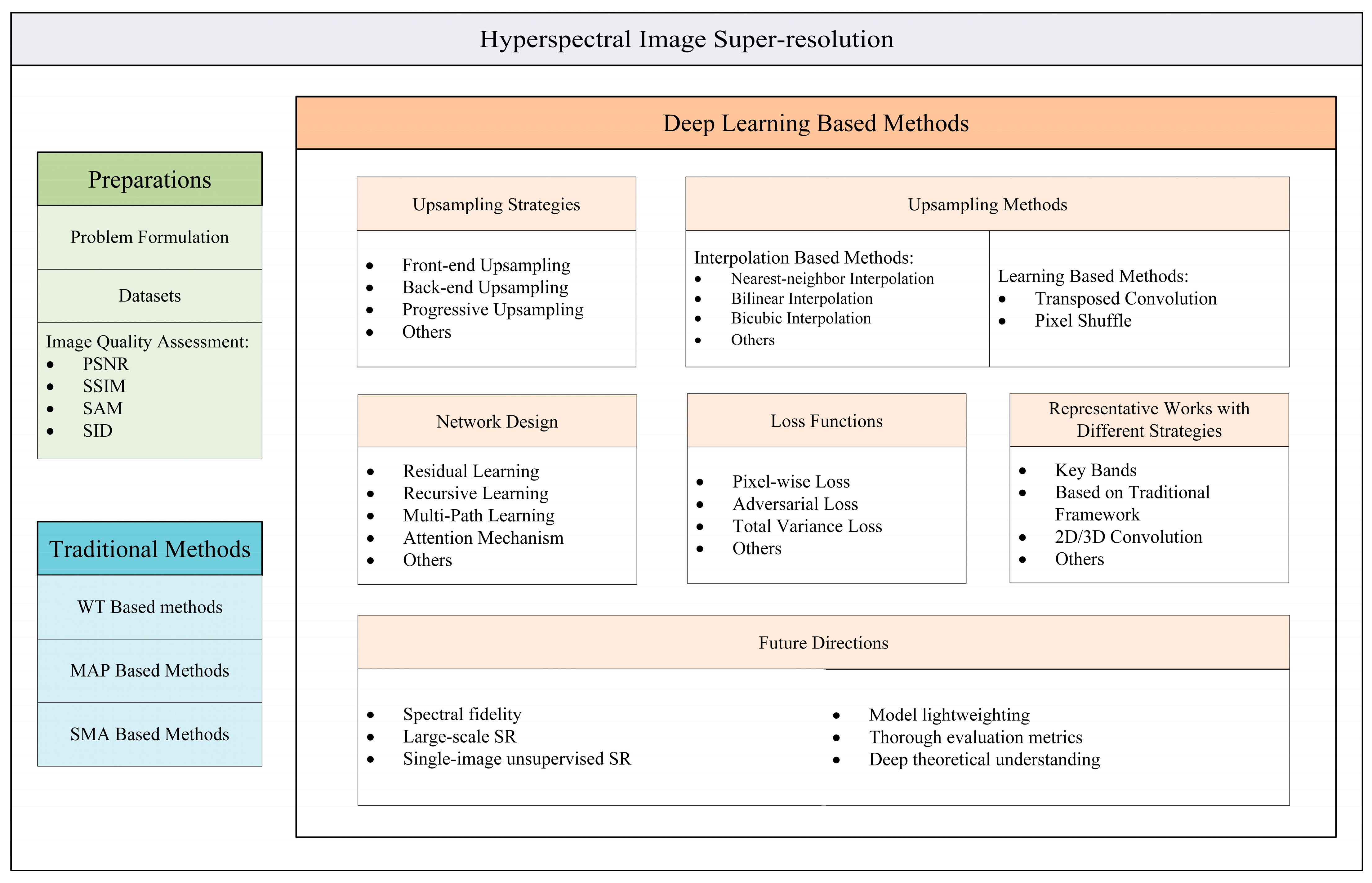
Figure 1. The main structure of this review.
Remotesensing 15 02853 g001
Figure 2. Diagram of CNMF algorithm for MSI and HSI data fusion. W/w and h/H are end-member matrices and abundance matrices resolved by LR HSI and HR MSI, respectively, where W and H are used to fuse the final HR HSI.
Remotesensing 15 02853 g002
Figure 3. Upsampling frameworks based on DL. The cube size represents the size of LR HSI and HR HSI. The blue ones denote convolutional layers, while the orange ones indicate upsampling layers.
Remotesensing 15 02853 g003
Figure 4. Learning-based upsampling methods. For input and output, each square represents a pixel.
Remotesensing 15 02853 g004
Figure 5. Network Design. In (d), different colors represent different weight information.
Remotesensing 15 02853 g005
Figure 6. Key band Strategy. The color of each band in the input represents how key that band is. The darker the color, the more important.
Remotesensing 15 02853 g006
Figure 7. Based on traditional framework strategy. The ellipse shows the traditional algorithms used to guide or constrain CNN.
Remotesensing 15 02853 g007
Figure 8. Diagram of two convolution modes. For input and output, each square represents a pixel. Black arrows show the direction in which the convolution kernel slides.
Remotesensing 15 02853 g008
Figure 9. The convergence of each model for the 3× SR during training.
Remotesensing 15 02853 g009
Figure 10. The visualization results for the 4× SR. Origin represents the labeled HR HSI.
Remotesensing 15 02853 g010
Figure 11. The spectral fidelity in the 3× SR case. The spectral curves of selected pixels from reconstructed images of 2D and 3D models and labeled HSI: the pixel locates at (15,15).
Remotesensing 15 02853 g011
Figure 12. The visualization results for the 4 × SR. Origin represents the labeled HR HSI.
Remotesensing 15 02853 g012
Figure 13. The spectral fidelity in the 4 × SR case. The spectral curves of selected pixels from reconstructed images of 2D and 3D models and labeled HSI: the pixel locates at (15,15).
Remotesensing 15 02853 g013
Table 1. List of Public Datasets for HSI SR.
DatasetAmountSizeWavelength (nm)Number of BandsSensorContents
CAVE32512 × 512400–70031Apogee Alta U260Stuff, Skin and Hair, Paints, Food and Drinks, etc.
Harvard771392 × 1040420–72031Nuance FX50 daylight images and 27 additional images.
Pavia Centre11096 × 715430–860102ROSISWater, Trees, Asphalt, Self-Blocking Bricks, etc.
Pavia University1610 × 340430–860103ROSISGravel, Trees, Asphalt, Self-Blocking Bricks, etc.
Washington DC11208 × 307400–2400191HYDICERoofs, Streets, Gravel Roads, Grass, Trees, Shadows.
Houston11905 × 349380–1050144ITRES CASI-1500Healthy Grass, Stressed Grass, Trees, Soil, Water, etc.
Chikusei12517 × 2335363–1018128Headwall Hyperspec-VNIR-CWater, Bare Soil, Grass, Forest, Row Crops, etc.
Table 2. Average Quantitative Comparisons on CAVE Dataset by Factor 2, 3 and 4.
Scale FactorModelPSNR ↑SSIM ↑SAM ↓Running Time/Epoch
SRCNN-2D41.5580.98743.24713.21
SRCNN-3D41.430.98842.81198.33
SRCNN-2D37.2430.97113.74920.41
SRCNN-3D36.6920.97013.512208.86
SRCNN-2D34.7650.95234.19933.96
SRCNN-3D34.2650.95073.982363.42
FSRCNN-2D40.8490.98623.62714
FSRCNN-3D40.3270.98653.15221.26
FSRCNN-2D37.2440.97044.18816.18
FSRCNN-3D36.7160.96963.80224.19
FSRCNN-2D34.9280.95324.67719.19
FSRCNN-3D34.2910.94924.61428.08
ESPCN-2D42.0830.98893.0510.975
ESPCN-3D125.9890.839720.48228.51
ESPCN-3D230.8040.92310.1278.87
ESPCN-3D334.680.96176.778142.52
ESPCN-2D37.4910.97263.6614.145
ESPCN-3D124.7280.769823.88730.65
ESPCN-3D228.9280.865313.1181.435
ESPCN-3D332.4550.92548.549139.155
ESPCN-2D35.0240.95564.12119.76
ESPCN-3D124.5450.732223.64135.865
ESPCN-3D228.3070.831214.35485.545
ESPCN-3D331.3030.900910.087143.045
The data highlighted in red in the table is the better data.
Table 3. Average Quantitative Comparisons on Pavia Centre Dataset by Factor 2, 3 and 4.
Scale FactorModelPSNR ↑SSIM ↑SAM ↓Running Time/Epoch
FCNN-2D36.0260.96144.84130
FCNN-3D34.2960.94814.823206.74
FCNN-2D31.1840.89096.07643.72
FCNN-3D30.2580.86956.039413.2
FCNN-2D28.0150.78967.578115.56
FCNN-3D27.8650.77937.378800.12
ERCSR-2D34.6020.95245.08113.95
ERCSR-3D33.8560.94525.166104.99
ERCSR-2D30.580.87886.50716.13
ERCSR-3D30.4050.88036.246121.8
ERCSR-2D28.4190.80497.76321.96
ERCSR-3D28.2750.79797.326150.32
The data highlighted in red in the table is the better data.
Table 4. Some Representative Models for HSI SR.
MethodUf.Um.Res.Rec.Mul.Att.Den.2D3DKeywords
3D-FCNN [18]Front.Bic. 3D Convolution
GDRRN [56]Front.Bic. Recursive Blocks
HSRGAN [61]Back.Sub. Generative Adversarial Network
SSPSR [64]Pro.Sub. Spatial–Spectral Prior
MCNet [62]Back.Dec. Mixed 2D/3D Convolution
BASR [77]Back.Dec. Band Attention
ERCSR [60]Back.Dec. Split Adjacent Spatial and Spectral Convolution
SGARDN [79]Back.Dec. Group Convolution
Interactformer [74]Back.Dec. Transformer
GELIN [71]Back.Dec. Neighboring-Group Integration
DRPSR [132]Pro.Bil. Deep Resonant Prior
“Uf.”, “Um.”, “Res.”, “Rec.”, “Mul.”, “Att.”, “Den.” represent upsampling frameworks, upsampling methods, residual learning, recursive learning, multi-path learning, attention mechanism, and dense connections, respectively.
Disclaimer/Publisher’s Note: The statements, opinions and data contained in all publications are solely those of the individual author(s) and contributor(s) and not of MDPI and/or the editor(s). MDPI and/or the editor(s) disclaim responsibility for any injury to people or property resulting from any ideas, methods, instructions or products referred to in the content.