Article

Characterizing Post-Fire Forest Structure Recovery in the Great Xing’an Mountain Using GEDI and Time Series Landsat Data

Research Center of Forest Management Engineering of State Forestry and Grassland Administration, Beijing Forestry University, Beijing 100083, China
*
Author to whom correspondence should be addressed.
Remote Sens. 2023, 15(12), 3107; https://doi.org/10.3390/rs15123107
Submission received: 18 April 2023 / Revised: 10 June 2023 / Accepted: 12 June 2023 / Published: 14 June 2023

Abstract

:
Understanding post-fire forest recovery is critical to the study of forest carbon dynamics. Many previous studies have used multispectral imagery to estimate post-fire recovery, yet post-fire forest structural development has rarely been evaluated in the Great Xing’an Mountain. In this study, we extracted the historical fire events from 1987 to 2019 based on a classification of Landsat imagery and assessed post-fire forest structure for these burned patches using Global Ecosystem Dynamics Investigation (GEDI)-derived metrics from 2019 to 2021. Two drivers were assessed for the influence on post-fire structure recovery, these being pre-fire canopy cover (i.e., dense forest and open forest) and burn severity levels (i.e., low, moderate, and high). We used these burnt patches to establish a 25-year chronosequence of forest structural succession by a space-for-time substitution method. Our result showed that the structural indices suggested delayed recovery following the fire, indicating a successional process from the decomposition of residual structures to the regeneration of new tree species in the post-fire forest. Across the past 25-years, the dense forest tends toward greater recovery than open forest, and the recovery rate was faster for low severity, followed by moderate severity and high severity. Specifically, in the recovery trajectory, the recovery indices were 21.7% and 17.4% for dense forest and open forest, and were 27.1%, 25.8%, and 25.4% for low, moderate, and high burn severity, respectively. Additionally, a different response to the fire was found in the canopy structure and height structure since total canopy cover (TCC) and plant area index (PAI) recovered faster than relative height (i.e., RH75 and RH95). Our results provide valuable information on forest structural restoration status, that can be used to support the formulation of post-fire forest management strategies in Great Xing’an Mountain.

1. Introduction

In the past three decades, over 2.5 million hectares of forests have been damaged by wildfires across the Great Xing’an Mountain region. These high intensity and frequency fire events have significantly altered forest structure, causing direct carbon emission from forest fire of about 0.48 Tg carbon year−1 [1,2,3]. Understanding post-fire forest structural response is crucial for sustainable forest management, as it impacts a wide range of ecosystem processes [4]. However, follow-up management such as removal of burned wood, replanting of seedlings, fertilization, and irrigation, etc., is often limited, leading to the gradual degradation of burned areas into large, low-productivity forests, particularly those initiated by lightning strikes in remote regions that are difficult to access. Therefore, characterizing post-fire forest structure recovery under various environmental conditions is challenging to achieve through field investigation alone.
Landsat data are the most commonly used source of imagery for detecting burn area, burn severity, and post-fire recovery at a regional scale [5,6,7]. These data provide more than four decades of land surface observations, giving a convenient and consistent approach for forest disturbance detection at long-term scales [8]. Spectral indices and tasseled cap transformations (TCT) have long been used to estimate influence factors (e.g., burn severity and pre-fire site conditions) related to vegetation recovery [9,10]. For example, DaSilva et al. [11] proposed a new application of TCT that improved the estimation of burn severity in semi-arid coastal regions. Viana-Soto et al. [1] established a support vector regression model using a set of Landsat-derived spectral indices and TCT to spatially extrapolate the LiDAR-derived tree height and canopy cover. However, despite the Landsat data being well-suited for describing the characteristic of forest fires, the lack of three-dimensional (3D) information limits the ability to assess the structural dynamic change induced by forest fires using Landsat data alone [12]. In contrast, light detection and ranging (LiDAR) sensors are capable of penetrating through vegetation and recording forest structural characteristics [13]. Therefore, the fusion of Landsat time series and LiDAR provides the opportunity to help bridge these knowledge gaps [14,15,16,17]. For example, Bolton et al. [12] utilized a time series of Landsat data to ascertain the conditions of burned areas, while airborne LiDAR was employed to evaluate the structural response. This approach allowed for the characterization of forest structure recovery subsequent to high-severity fires. Additionally, Landsat imagery can be used to extrapolate LiDAR-derived structural variables, proving to be an effective approach to describe post-fire forest structure recovery. García et al. [17] demonstrated the feasibility of extrapolating LiDAR-derived structural variables using Landsat images over time.
Space-based LiDAR data directly provide abundant information on vertical vegetation structure, including canopy structure [18], canopy height [19], biomass [20], and species richness [21], exceeding the capabilities of ground-based in situ observations. In September and December 2018, a new space-based laser altimetry mission, the Global Ecosystem Dynamics Investigation (GEDI) instrument, was launched. It consisted of three lasers that produced a total of eight ground transects, with each transect sampling eight footprints of approximately 25 m in size. These footprints were spaced approximately every 60 m along the track, allowing for global data collection between latitudes 51.6°N and 51.6°S. Such wide coverage of GEDI data offers unprecedented opportunities to characterize global ecosystem structure and dynamics and fundamentally improve the quantification and understanding of Earth’s carbon cycle and biodiversity [22]. The integration use of GEDI measurement and Landsat imagery has been explored to detect forest structure change. Francini et al. [23] integrated Landsat imagery and GEDI metric to detect biomass increase following forest disturbances across Italy. Although there have been a variety of GEDI-based approaches in mapping forest structures, long-term forest structure recovery following fire has seldom been assessed by GEDI data due to the limitation of data acquisition time. Space-for-time substitutions, also known as ergodic gradient studies, are often used for vegetation status estimation during the recovery process in the absence of long-term data sets [24], that provide an opportunity to observe successional changes in the forest structure in Great Xing’an Mountain.
This study aimed to assess the capability of integrating GEDI metrics with Landsat time-series data to capture the dynamics of post-fire forest structure across the Great Xing’an Mountain under varying site conditions. We constructed a 25-year structural development chronosequence to explore the following questions: (1) Do GEDI metrics capture the recovery of forest structure using the space-for-time substitution method? (2) How do burn severity and pre-fire canopy cover affect forest structure recovery and pattern of succession after a fire? To address the first question, we calculated the percentage of GEDI metrics of burned patches to the corresponding unburned patches. The second question was addressed by integrating Landsat time-series data to assess burn severity level and pre-fire canopy cover.

2. Materials and Methods

2.1. Study Area

The study area (50°10′–51°6′N, 120°12′–122°53′E) is located in the northwest of the Great Xing’an Mountains. The forests in Great Xing’an Mountain were originally occupied by the Gmelin’s larch (Larix gmelinii), accounting for 80% of the cover [25]. The primary deciduous broadleaf species following fire disturbances is white birch (Betula platyphylla), which is usually a pioneer successional species [26]. In this region, wildfires are generally characterized by frequent surface fires and infrequent stand-replacing crown fires, with fire recurrence intervals varying from 30 to 120 years [26]. According to the fire registration statistics of the Forestry Bureau, since the 1960s, as many as 126 fires have been recorded in this area, including 21 major forest fires. In this study, we focused on the fire events that occurred from 1987 to 2019 within the spatial distribution range of GEDI data (i.e., within 51.6°N latitude).

2.2. Dataset and Preprocessing

2.2.1. GEDI Data

To describe the post-fire forest structure dynamics, the GEDI level 02A (L2A) and level 02B (L2B) product data over the study area were obtained for the growing seasons of June to August from 2019 to 2021. The general information for each product is shown in Table 1. L2A/L2B products covering the study area were available from the NASA/USGS Land Processes Distributed Active Archive Center (LPDAAC, https://e4ftl01.cr.usgs.gov/GEDI/) (accessed on 23 November 2022). We then used a Python script (GEDI Subsetter) to spatially clip the GEDI product and output the desired parameters as GeoJSON files for further visualization and analysis. To select the highest quality data, the GEDI data were further filtered to remove abnormal waveforms for measuring forest structure. The quality of each GEDI shot is checked by a “quality flag” and “sensitivity”, that allows one to easily remove erroneous or lower-quality waveforms [27]. To eliminate the effect of environmental noise and steep slope, we selected only the power beam mode (i.e., full-strength lasers) at night with quality flag = 1, beam sensitivity ≥ 0.95, and slope ≤ 15°. A total of 90,472 sample footprints containing valid measurements were used for subsequent analyses.

2.2.2. Landsat Data

Annual composites of Landsat TM and OLI surface reflectance for the period 15 June–15 August 1986–2020 were generated through the Google Earth Engine (GEE) platform using a median selection process [28], filtering by cloud cover (less than 20%). To reduce the differences among the spectral characteristics of Landsat ETM + and OLI datasets, inter-sensor harmonization was conducted by the LandsatLinkr package in R language developed by Vogeler et al. [29]. A set of spectral indices were computed to assess burn severity and retrieve pre-fire tree canopy cover: the normalized difference vegetation index (NDVI) [30], the enhanced vegetation index (EVI) [31], the soil adjusted vegetation index (SAVI) [32], normalized difference moisture index (NDMI) [33] and the normalized burn ratio (NBR) [34]. Tasseled cap transformations (brightness, greenness, and wetness) were calculated using the coefficients derived by Baig et al. [35].

2.2.3. Tree Canopy Cover

The Global Forest Cover Change GFCC dataset available for four epochs centered on the years 2000, 2005, 2010, and 2015 was obtained from the Google Earth Engine (GEE) platform. This dataset contains estimates of the percentage of horizontal ground in each 30 m pixel covered by woody vegetation greater than 5 m in height that are based on Landsat satellite images. To restrict the analysis to areas that were forested prior to burning, according to Bolton et al. [12], we determined the 20–50% and greater than 50% canopy cover classes as “open” and “dense” forests, respectively.

2.3. Fire Detection and Burn Severity Classification

The detection of burn patches was conducted by yearly-time series of Landsat data. To avoid the interference signal due to phenological differences, only the available data within the growing seasons (15 June–15 August) were selected for annual composites. The change in NBR from bi-temporal imagery, known as the dNBR (Equation (1)), has been shown to correlate well with both burn area and burn severity detection [5,36]. Therefore, the dNBR at each composite image time-step was calculated for detecting burned patches.
d N B R = N B R p r e N B R p o s t
When identifying burned areas using dNBR, we applied a threshold to prevent subjective decisions by utilizing the Otsu method [37]. The Otsu algorithm uses bimodal histogram processing to create a binary image (i.e., only two classes of pixels: burned and unburned) and finds the optimal threshold that minimizes the intra-class variance [35]. Specifically, the Otsu algorithm assumes that the difference image has L grey levels [1, 2, …, L]. According to the Otsu algorithm, the image can be divided into the burned and unburned area classes by a threshold t (1 < t < L). The between-class variance g is defined as:
g t = w b , t × w n b , t × μ b , t μ n b , t 2
where w b and w n b represent the proportions of burned and unburned areas. μ b and μ n b are the mean values for two class samples. Finally, the optimal threshold T maximizing the interclass variance is estimated by an iterative process:
T = arg max g t
To remove small-area disturbances and image noise, we applied multiple noise-filtering steps. The first filtering removed non-forest regions using the pre-fire GFCC values of less than 20%. The second filtering removed the small burned patches by calculating the burned areas less than 10 ha. Additionally, areas that burned more than once between 1986 and 2020 were also not included, as the structural response of vegetation could be more complicated in these cases. The process of Otsu analysis and noise filtering was conducted through the GEE platform.
Burn severity is defined as fire-induced changes in vegetation structure and assessed by a certain amount of time having elapsed after a fire, which is directly determined by the rate of post-fire forest regeneration [38,39]. After burned patches detection, four discrete levels of high severity (dNBR ≥ 0.6), moderate severity (0.6 > dNBR ≥ 0.3), low severity (0.3 > dNBR ≥ 0.1), and unburned (dNBR < 0.1) for each fire site were further classed using the thresholds of the dNBR that have been proposed by Chu et al. [25] for the burn severity assessment in Great Xing’an region.

2.4. The Pre-Fire Tree Canopy Cover

To ensure that the analysis was restricted to forested areas and differentiate the structural response to pre-fire canopy cover conditions, information on the canopy cover prior to the fire was required. A classification model was developed for three canopy cover classes (non-forest: 0–20%, open patches: 20–50%, and dense patches: >50%) based on GFCC and pre-fire Landsat data. The training samples on canopy cover were derived from multiple target dates of GFCC products in the years 2000, 2005, 2010, and 2015. To ensure that the value distributions of the training set accurately represent our study area, we generated a total of 1000 random sample points within fire perimeters that occurred after the year 2000. These points were selected to be more than 50 m away from the polygon edge. Sample points were located >100 m apart to minimize the effect of spatial autocorrelation. These samples would be further used as a point of interest to extract the predictive variables for RF model construction.
In order to encompass the diversity of vegetation characteristics, a series of spectral bands, spectral indices, and TCT were used to develop the RF classification. RF is a machine learning technique that exhibits improved performance in dealing with high-dimensional regression issues [40]. In this study, a total of 14 candidate variables were used for the RF model establishment (Table 2). After the best variable subset has been selected, we established an RF regression model to estimate the canopy cover. The RF regression algorithm is based on bootstrap resampling and the decision tree method, which is controlled by three key parameters: the number of decision trees (Ntree), the number of node splits per tree (Mtry), and node size. The accuracy of model prediction was validated by independent samples using the coefficient of determination (R2) and the root means square error (RMSE). The R-package Random Forest (version 4.6-14) regression procedure was used to complete this analysis.

2.5. Assessing Post-Fire Structural Response to Fire

2.5.1. Structural Metrics from GEDI Data

The GEDI products provide high-quality measurements of forest vertical structures that have been widely used to produce high-accuracy maps of key forest structure attributes (e.g., tree height, canopy cover, plant area index, biomass, etc.) [19,20,22,23]. The analysis focuses on GEDI metrics that describe tree height and canopy profiles, as these metrics are commonly used to estimate carbon stock and assess tree mortality resulting from fire disturbances [1,12]. Each metric is separately derived from the information stored in footprint datasets of processing levels: L2A and L2B. The L2A product is primarily composed of 100 relative height (RH) metrics (RH0, RH1, … RH100), corresponding to the height of waveform energy cumulative from 0% to 100%. In this study, the 75th (RH75) and 95th (RH95) height percentile were assessed as stand height metrics, because the RH95 metric has the highest correlation with the forest canopy height [19] and the RH75 is more likely related to vegetation regrowth [12]. As for the canopy profiles, the L2B product stores the metrics including total canopy cover (TCC), plant area index (PAI), and foliage height diversity (FHD). Among them, the TCC is the percent of the ground covered by the vertical projection of canopy structures (i.e., leaves, branches, and stems) [41]. PAI describes the horizontal projected area of plant elements per unit of ground area (m2m−2) within a volume of the canopy [41], and the PAI at any given height can be calculated from waveform data with the equations:
g a p z , θ = 1 R v z R v 0 + R g × ρ v ρ g ,
P A I = 1 ln P g a p θ ln P g a p θ G θ Ω θ ,
where R v z is the integral of reflected energy from canopy elements from the canopy top down to the given height (z). R g is the integral of reflected energy from the ground. Δ z is the height increment at which PAI is calculated. Canopy-to-ground reflectance ratio ρ v / ρ g , a nadir view angle ( θ ), a spherical leaf angle distribution ( G θ ), and a random spatial distribution of canopy elements ( Ω θ ) are defaulted as 1.425, 0, 0.6, and 1, respectively. FHD is a canopy structural index that describes the vertical heterogeneity of foliage profile [41].
F H D = i N i × log N i ,
where Ni is the proportion of the vertical PAI profile that lies in the ith of the chosen horizontal layers.

2.5.2. Construction of Post-Fire Forest Structural Chronosequence

Site conditions and pre-fire stand composition have been shown to strongly influence post-fire stand succession patterns [42,43]. Therefore, we, respectively, assessed post-fire forest structure response to different burn severity levels and pre-fire canopy cover conditions. To avoid the complex interaction between burn severity and canopy cover conditions, we only analyzed forest structure response to different burn severity levels within the pre-fire dense forest patches and forest structure response to pre-fire canopy cover conditions in high burned severity patches. As the GEDI data were limited to the acquisition time after 2019, the chronosequence of forest structural recovery consisted of GEDI lidar metrics (i.e., RH95, RH75, TCC, PAI, and FHD) of different fire events from 1987 to 2019 using space-for-time substitution. To reduce the bias of stand growth induced by different site conditions, each LiDAR metric for neighboring unburned patches was also calculated for each fire event. By applying the canopy cover classification to each pre-fire imagery, the selected unburned patches should be spectrally similar to the burned forest patches prior to the fire. We used the percentage indices that were computed from the GEDI metrics using the selected burned and unburned patches (Equation (7)):
P I L M = i = 1 n L M b u r n e d , i / n j = 1 m L M u n b u r n e d , j / m × 100 ,
where P I L M is the percentage indices of a given GEDI LiDAR metric, and L M b u r n e d , i and L M u n b u r n e d , i represent the value of the GEDI metric of burned and unburned patches. n and m represent the number of GEDI samples for burned and unburned patches. Then, we calculated the year since the fire (YSF) for each fire by subtracting the year that the fire occurred in from the year of GEDI data acquisition (2019, 2020, and 2021). The average values of these percentage indices were calculated for each fire and then we further counted the average and standard deviation every 5 years as indicators of the levels of recovery in relation to YSF.

3. Results

3.1. Fire Detection and Burn Severity Mapping

Over 80 fire events were detected totaling over 480,000 hectares of forest burn areas across Landsat scenes within the GEDI data acquisition range from 1986 to 2019 (Figure 1). Burned areas are concentrated and distributed in the latitude range of 51°N to 52°N, especially in the west and east of Great Xing’an Mountain.
The examples of burned severity maps with GEDI footprints are shown in Figure 2. Most of the fires appeared in red tones indicating that a high proportion of high burn severity class has occurred (Table 3, Figure 2). These maps were used to stratify the GEDI samples for tracking the temporal patterns of the forest at different burn severity levels. RH75 metrics tend to be lower in the burned areas, especially in the high burn severity class. These GEDI footprints were also used as a region of interest to extract burn severity levels and pre-fire canopy cover openness for further statistics.
The annual burn classifications showed different spatiotemporal distribution patterns of burned area (Figure 1 and Figure 3). For instance, in the period of 1987–1997, fewer fire patches with a wide range of sizes and scattered distribution occurred (Figure 1). During the time period of 1998–2008, fire incidents occurred annually, resulting in an overall increase in the total burned area (Figure 3). Fires were concentrated in the west and east side of Great Xing’an Mountain, especially in 2003 and 2006 (Figure 1). During the period from 2009 to 2019, there was a decrease in the burned area. However, smaller patches of fire were still evident within the Great Xing’an Mountain (Figure 1). Examining the dynamic trends in burned areas over 11-year intervals, we observed that the burned area increased from 70,623 hectares in the period of 1987–1997 to 380,832 hectares in 1998–2008. However, it subsequently decreased to 37,522 hectares in the period of 2009–2019 (Table 3; Figure 3).

3.2. Tree Canopy Cover Estimation

Figure 4 compares the predicted canopy cover (CC) using the RF model and the reference CC using the independent GFCC data. The model-estimated CC is consistent with the referenced CC with relatively high precision (R2 = 0.71, RMSE = 8.6). We then categorized the canopy cover into non-forest (CC < 20%), open forest (20% < CC < 50%), and dense forest (CC > 50%). Produce accuracy (PA), user accuracy (UA), and overall accuracy (OA) were used to evaluate the classification of forests into the three categories described above (Table 4). This resulted in an overall cross-validated accuracy of 69.6%. Among the three classes, the non-forest class has higher PA (71.8%) and UA (77.7%) than the open forest class (PA = 70.3%, UA = 66.6%) and dense forest class (PA = 67.2%, UA = 69.0%).

3.3. Assessment of Forest Structure Recovery

Due to the small number of detected fire events prior to 1995 (Figure 3), the fires of 25–35 YSF were not used in the construction of the forest structure recovery sequence. We estimate the mean and standard deviation for each YSF group under different site conditions. These groups are arranged in chronological order to obtain recovery sequences.

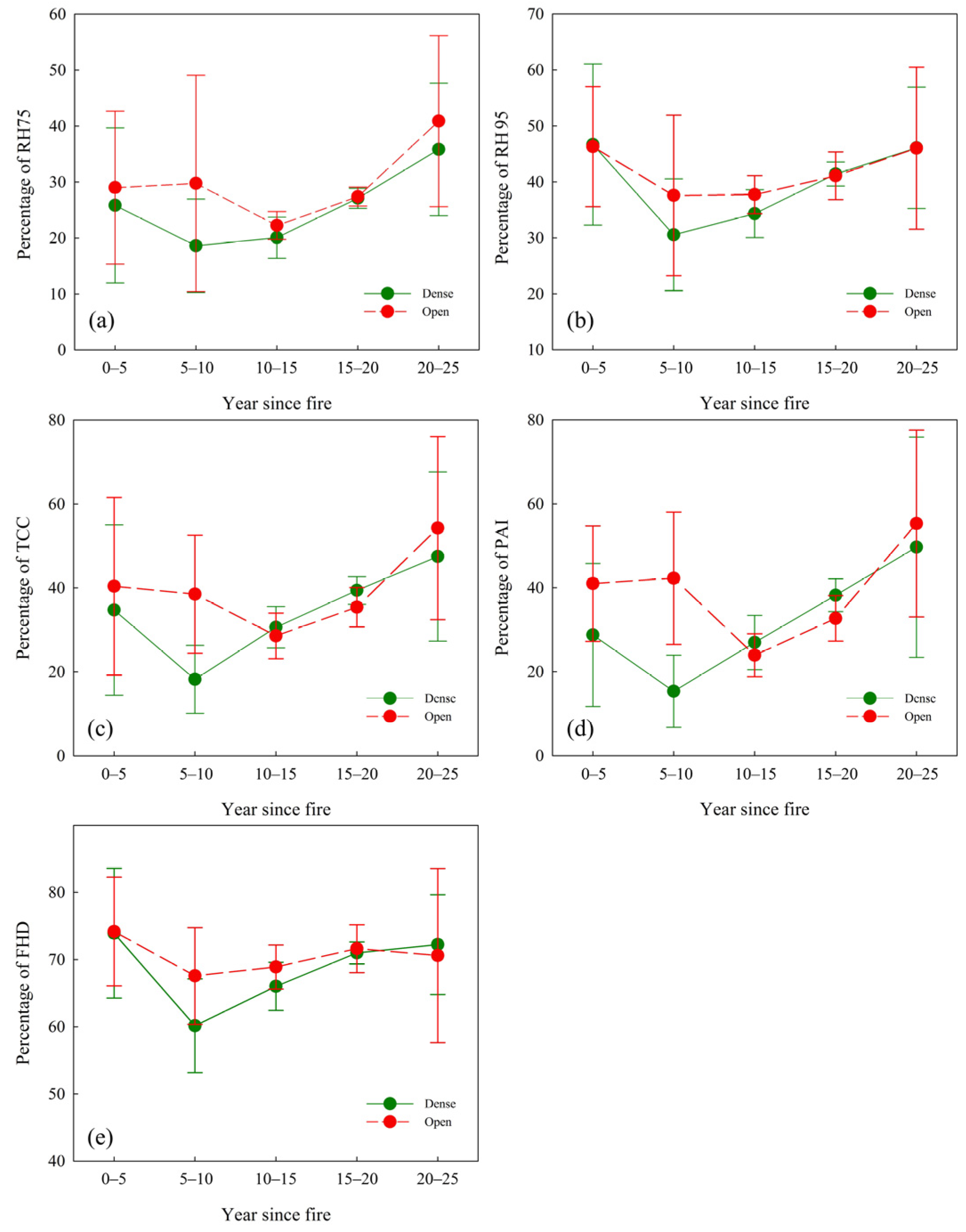
3.3.1. Forest Structure Recovery under Different Pre-Fire Canopy Cover

Two stand height indices showed slightly different recovery trends (Figure 5a,b). The percentage of RH75 was the lowest at 5–10 YSF for dense forest patches and 10–15 YSF for open forest patches, while the percentage of RH95 was the lowest at 5–10 YSF for both dense and open forest patches. Compared with RH95, RH75 showed a delayed recovery trend with no significant increase until 15 YSF. For open forests, the difference between 0–5 YSF and 5–10 YSF groups of RH75 was less pronounced while RH95 showed an obvious decline. Overall, the extent of RH75 and RH95 recovery is not more than 60% in the observed YSF.
Three canopy indices were used to describe the pattern and extent of forest structure recovery (Figure 5c–e). TCC and PAI indicate similar recovery trends (Figure 5c,d) for both open and dense forests. The open forest indicates a delayed recovery with percentages lowest at 10–15 YSF compared with 5–10 YSF for dense forest. The dense forest recovery trend is faster in the 5–10 YSF and 15–20 YSF periods but slower between the 15–20 YSF and the 20–25 YSF periods. Although the declines of TCC and PAI are higher than stand tree height, TCC and PAI have significantly faster recovery trends than the tree height indices and increased sharply between 15–20 and 20–25 YSF for open patches. In contrast, FHD has the smallest change relative to an unburned area with the lowest percentage of 53% for dense forests and 57% for open forests. FHD of the open forest shows no significant recovery trend after a fire compared with the dense forest.
Among all percentage indices, we found on average, greater losses and faster recoveries in dense forest patches relative to open forest patches in the early successional stage (10–20 YSF), and delayed recovery in all percentage indices for both open and dense patches, i.e., the recovery trend was not detected until 10 years after the fire. The standard deviations (SD) of the various indices were lower for the 10–20 YSF compared with 0–10 YSF and 20–25 YSF.

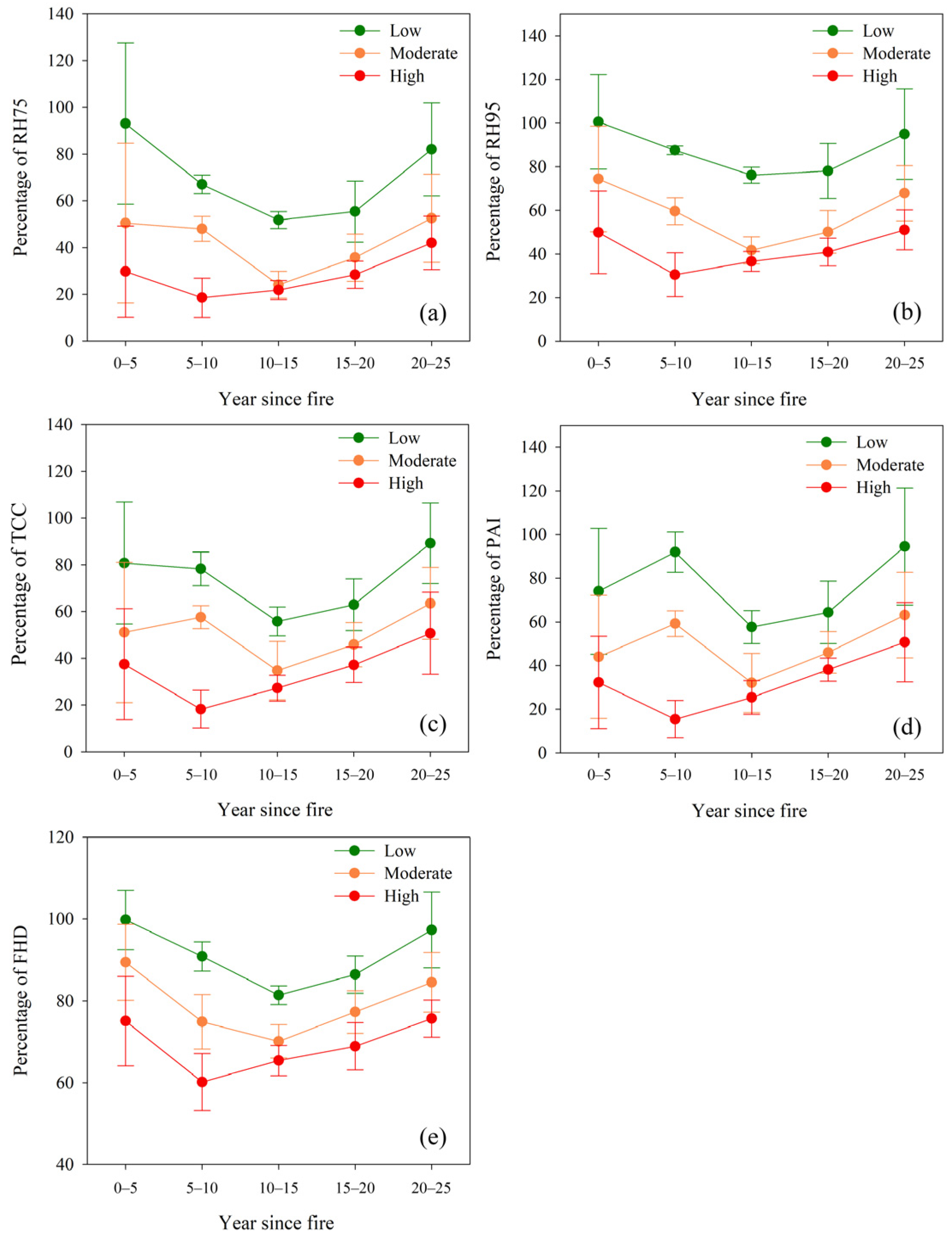
3.3.2. Forest Structure Recovery under Different Burned Severity

The indicated forest structure recovery under different levels of burned severity is displayed in Figure 6. The percentage value of RH95 is generally greater than that of RH75, and the values of RH95 remained significantly higher (i.e., 80–120%) at 0–5 YSF in low burned severity patches. For patches with low and moderate severity, the lowest values are found in the 10–15 YSF group, while for patches with high severity, the lowest values are observed in the 5–10 YSF group.
For three foliage indices, we found low and moderate severity TCC and PAI did not decrease significantly between 0–5 and 5–10 YSF, and there was an increase for PAI. Similar to the stand height indices, for percentage indices of TCC, PAI, and FHD, the lowest value was in the 10–15 YSF group for low and moderate burn severity patches and the lowest value was in the 5–10 YSF for high severity patches. The percentage indices of TCC and PAI values were lower when compared to the stand height indices.
There were differences in the average structure recovery patterns amongst the three burn severity classes. In the 25–year chronosequence, the percentages indices were relatively high for low burned severity, and then decreased for moderate and then high severity classes. We found that the low and moderate-burned patches had a later recovery trend than high-burned patches. The average increase (AI) in indices was highest for low burned severity (AI = 27.06%), followed by moderate (AI = 25.7%) and high burned (AI = 18.7%) severities between 10–15 YSF and 15–20 YSF. Standard deviations were relatively high in 0–5 YSF and 20–25 YSF.

4. Discussion

4.1. Forest Structural Response to Pre-Fire Canopy Cover

Forest structure immediately after the severe fire is usually characterized by standing dead wood and canopies remain relatively open for a short period after the fire [44]. Johnstone et al. [45] found that it might take about 3–7 years for most trees to become established following the fire at boreal sites. Therefore, instead of detecting new tree growth, GEDI metrics were sensitive to the loss of residual structure during the early post-fire successional stage, as further decreasing trends were observed both in the structure of tree height and canopy structure (Figure 5). With new trees growing to a certain height, the subsequent increasing trends start to be captured by the percentage of GEDI metrics, forming a concave trajectory of forest structure recovery. This result was consistent with Bolton et al. [12] who found a similar concave recovery trajectory for canopy cover and stand height in high-severity burn patches. The field photos collected from the 2018 historical fire investigation across study areas can also explain this concave recovery trajectory in relation to percentage indices (Figure 7). Within eight years of the fire (Figure 7a–c), we can see the residual structure such as dead wood and snags begin to fall, and the new tree regrowth starts from the understory stratum, demonstrating the decreasing trends in relation to tree height (RH75 and RH95) and canopy profile (TCC, PAI, and FHD). Fifteen years after the fire (Figure 7d–f), the new sprout trees gradually grew from open space to canopy closure, indicating the increasing trends of tree height (RH75 and RH95) and canopy profile (TCC, PAI, and FHD) in this period.
Dense and open patches have a similar percentage of GEDI metrics loss in the first five years, while indices were further decreased more for dense patches than for open patches. The probable reason is that the indices we used are relative to the unburnt patches with similar pre-fire canopy cover conditions, implying that as residual structure in high burn severity patches gradually collapses, forming open spaces, dense patches have a greater proportion of structural loss compared to open patches. Differences in recovery rates between dense and open patches were further confirmed by percentage indices. Dense patches exhibited faster growth and recovery compared to open patches in the subsequently increased trends, possibly because pre-fire canopy attributes can reflect growth environment so that more productive sites with higher canopy cover reestablish cover more quickly after fire than less productive sites [46]. Bolton et al. [12] also proved faster tree recovery under pre-fire dense canopy cover conditions than that under open conditions. These findings demonstrate that forest canopy cover prior to fire is an important indicator of structural response post-fire, limiting the growth of new trees following the fire.
Canopy cover metrics (TCC and PAI) and tree height metrics (RH75 and RH95) displayed a different response to disturbance in our observed time sequences. The result indicates that TCC and PAI can recover more with a higher value than RH75 and RH95, which is likely explained by the rapid development of foliage of trees [12] while vertical tree growth and biomass gains are much slower processes [47,48]. Martín-Alcon et al. [49] and Matasci et al. [50] both agree on the marked differences in the evolution of canopy cover and height estimates in boreal forests, where tree cover reached pre-fire values earlier but canopy height did not recover. As for the recovery of the vertical profile, high FHD value in forest ecology often results from more complex forest structures (e.g., caused by multiple canopy layers) [41]. Therefore, the recovery trend of FHD is slow in the observed successional stage, as trees are even-aged and maximum tree size is limited by a short growth period [51]. Johnston et al. [52] also found early successional stands to be less FHD than late successional stands.

4.2. Forest Structural Response to Burn Severity

Burn severity is another key factor that determines the survival rate of trees and interacts with the physical environment affecting post-fire forest structural recovery [53,54]. Different degrees of structure loss in three levels of burn severities were further confirmed by GEDI metrics, as the percentage values of GEDI metrics are highest in low burn severity levels, followed by moderate and low burn severity. In terms of the recovery trajectory, we also found a concave trend for low- and moderate-severity patches with the lowest value for 10–15 YSF, indicating that regardless of the severity of the fire, GEDI metrics are more sensitive to residual structure decomposition in the short term after the fire than vegetation recovery. Karna et al. [46] also found a persistent reduction in canopy cover of eucalypt forests under different burn severities for at least seven years, especially for moderate- and high-burn severity. Further decreasing trends were observed between 5–10 and 10–15 YSF in low- and moderate-severity patches. This may be attributed to the fact that, compared to high-severity patches, low- and moderate-severity patches retain a greater number of live trees in their canopy structure, which restricts the regeneration of new trees and the decomposition of residuals in the short-term following the fire. As a result, it takes a longer time for GEDI metrics to detect an increasing trend. On the other hand, post-fire artificial regeneration measures, such as residual wood removal and replanting, are more likely to be implemented in severely burned patches. This difference can be further confirmed by the field observation in Figure 8. We can see that the residual structures (i.e., fallen logs, snags) still remain in the moderate burn severity plot (Figure 8a) and new trees tend to grow faster in the high burn severity plot (Figure 8b). In terms of dynamic change in percentage of GEDI metrics, post-fire tree height in three burn severity levels displayed that RH75 has a lower percentage value than that of RH95. This is consistent with the widespread observation that fire thins from below by removing smaller trees [55,56]. Besides, we noticed that the percentage TCC and PAI of low and moderate burn severity patches showed no difference or even an increasing trend between 0–5 and 5–10 YSF groups and then decline between 5–10 and 10–15 YSF groups, probably because the canopy foliage recovered faster from live trees in the short-term after the fire while the dead residual structure would continue to decompose after 10 years since the fire.

4.3. Limitation

The application used of GEDI metrics for post-fire forest recovery quantification is limited. We only used the GEDI dataset collected from 2019 to 2021, and the statistical results of percentage indices are influenced by the number of fire events within one YSF group. In terms of chronosequence construction, our result showed that these indices have relatively high variability in 0–5 YSF, 5–10 YSF, and 20–25 YSF groups. Although we have controlled variables in the analysis of post-fire forest structure recovery, the use of space-for-time substitution method along a broad latitudinal gradient from 47.27° to 51.66° would lead to the high variability of percentage indices in one YSF group. On one hand, our structure recovery trajectory might be compounded by differences in climatic conditions across the landscape [57], causing a great difference in vegetation regrowth over the same period of time. For example, Jiang et al. [57] revealed that the radial growth of larch might be decreased by warmer temperatures and decreasing precipitation. Similarly, tree regeneration after disturbances could be limited under post-fire drought events since droughts constrain seedling establishment and growth [58]. On the other hand, variability in species composition across the landscape could also contribute to the structural differences within one YSF group. As post-fire tree establishment is strongly linked to pre-fire species composition [43,59], structural differences between stands could redevelop during the early stages of succession. Besides, GEDI data cannot provide wall-to-wall maps of the forest stand (Figure 2), implying that discrete GEDI data have limitations in describing the complete characteristics of a burn area, leading to bias in characterizing the post-fire forest structure change.
In addition to the uncertainties due to the use of GEDI data by space-for-time substitution method, the post-fire forest structure recovery can be also distorted by the determination of recovery drivers. The post-fire structural development depends largely on burn severity, due to its relation to tree seedling densities after fire, depending on pre-fire vegetation composition, seedling mortality, and reestablishment processes [60,61,62,63]. In this study, the assessment of burn severity level was accomplished by applying a fixed dNBR threshold since many researchers found a high relationship between dNBR and burn severity [36]. However, a number of factors can confound the distinction of burn severity levels such as vegetation characteristics, the acquisition time of pre- and post-fire imagery, and soil properties [16,64]. Moreover, it should be mentioned that burn severity might be easily underestimated, especially for low and moderate levels, since burn severity assessments based on the spectral index were mainly determined by upper canopy spectra and the actual damage of under- or mid-story vegetation cannot be captured correctly [65]. Therefore, when a single threshold of dNBR was applied to classify the burn severity level across a wide range of areas, the confusion of severities may be included in this analysis, leading to the variability in structural responses observed. The classification accuracy of pre-fire patches into dense or open forests based on Landsat and GFCC data could also contribute to the variability in structure response. In our study, the values of PA and UA were lower than 80%, indicating that there is mutual confusion among different pre-fire patch types in the classification results.

5. Conclusions

In this study, we assessed post-fire forest structure development after fire across the Great Xing’an Mountain region using a combination of time series Landsat data and GEDI data. Our results suggest that burn severity and pre-fire canopy conditions have a strong influence on post-fire stand development. In terms of burn severity, the percentage of each metric is highest in low burn severity followed by moderate and high burn severity. A more delayed recovery was found in low and moderate burn severity but with a faster recovery when compared to high burn circumstances. In terms of pre-fire canopy conditions, dense forests displayed a larger loss but faster growth and recovery than open forests. Additionally, noticeable different recovery patterns between stand mean height (i.e., RH95) and canopy cover metrics (i.e., TCC and PAI) were found in high burn severity patches, as the percentage of TCC and PAI recovered more than that of tree height within the observed time sequence. The largest proportion of PAI and TCC is over 75% in the 20–25 YSF group while RH95 is less than 60%. Although the 25-year chronosequence is composed of multiple fire events using the space-for-time substitution method, an obvious transition from open canopies of residual structure to canopies closed by new trees could be captured by GEDI metrics. As the amount of GEDI data increase, a long-term observation of post-fire forest structural recovery for a specific site can be obtained, avoiding the need to resort to space-for-time substitutions. Our work provides the first step in characterizing the post-fire succession of forest structure. It can provide useful information about forest structural restoration status to support the post-fire restoration activities in Great Xing’an Mountain.

Author Contributions

Conceptualization, S.L. (Simei Lin); methodology, S.L. (Simei Lin) and H.Z.; software, S.L. (Simei Lin), S.L. (Shangbo Liu), G.G., and H.Z.; investigation, S.L. (Simei Lin); writing—original draft preparation, S.L. (Simei Lin), H.Z., and G.G.; writing—review and editing, H.H. and L.L.; supervision, H.H.; project administration. All authors have read and agreed to the published version of the manuscript.

Funding

This research was funded by the Key Program of National Natural Science Foundation of China (No. 42130111).

Data Availability Statement

Publicly available datasets were analyzed in this study. The data sources and access links are indicated in the text.

Acknowledgments

We thank NASA/USGS Land Processes Distributed Active Archive Center to provide the free data.

Conflicts of Interest

The authors declare no conflict of interest.

References

  1. Viana-Soto, A.; García, M.; Aguado, I.; Salas, J. Assessing post-fire forest structure recovery by combining LiDAR data and Landsat time series in Mediterranean pine forests. Int. J. Appl. Earth Obs. Geoinf. 2022, 108, 102754. [Google Scholar]
  2. Zhang, Y.; Hu, H.Q.; Wang, Q. Carbon emissions from forest fires in great Xing’an mountains from 1980 to 2005. Procedia Environ. Sci. 2011, 10, 2505–2510. [Google Scholar] [CrossRef] [Green Version]
  3. Bowman, D.M.J.S.; Williamson, G.J.; Abatzoglou, J.T.; Kolden, C.A.; Cochrane, M.A.; Smith, A.M.S. Human exposure and sensitivity to globally extreme wildfire events. Nat. Ecol. Evol. 2017, 1, 58. [Google Scholar]
  4. Kane, V.R.; North, M.P.; Lutz, J.A.; Churchill, D.J.; Roberts, S.L.; Smith, D.F.; McGaughey, R.J.; Kane, J.T.; Brooks, M.L. Assessing fire effects on forest spatial structure using a fusion of Landsat and airborne LiDAR data in Yosemite National Park. Remote Sens. Environ. 2014, 151, 89–101. [Google Scholar]
  5. Hawbaker, T.J.; Vanderhoof, M.K.; Beal, Y.J.; Takacs, J.D.; Schmidt, G.L.; Falgout, J.T.; Williams, B.; Fairaux, N.M.; Caldwell, M.K.; Picotte, J.J.; et al. Mapping burned areas using dense time-series of Landsat data. Remote Sens. Environ. 2017, 198, 504–522. [Google Scholar]
  6. Quintano, C.; Fernandez-Manso, A.; Roberts, D.A. Burn severity mapping from Landsat MESMA fraction images and Land Surface Temperature. Remote Sens. Environ. 2017, 190, 83–95. [Google Scholar]
  7. Chu, T.; Guo, X. Remote sensing techniques in monitoring post-fire effects and patterns of forest recovery in boreal forest regions: A review. Remote Sens. 2013, 6, 470–520. [Google Scholar]
  8. Wulder, M.A.; Masek, J.G.; Cohen, W.B.; Loveland, T.R.; Woodcock, C.E. Opening the archive: How free data has enabled the science and monitoring promise of Landsat. Remote Sens. Environ. 2012, 122, 2–10. [Google Scholar]
  9. Frazier, R.J.; Coops, N.C.; Wulder, M.A.; Hermosilla, T.; White, J.C. Analyzing spatial and temporal variability in short-term rates of post-fire vegetation return from Landsat time series. Remote Sens. Environ. 2018, 205, 32–45. [Google Scholar]
  10. Zhang, Q.; Homayouni, S.; Zhao, P.; Zhou, M. Burned vegetation recovery trajectory and its driving factors using satellite remote-sensing datasets in the Great Xing’An forest region of Inner Mongolia. Int. J. Wildland Fire 2023, 32, 244–261. [Google Scholar]
  11. DaSilva, M.D.; Bruce, D.; Hesp, P.A.; Miot da Silva, G. A New Application of the Disturbance Index for Fire Severity in Coastal Dunes. Remote Sens. 2021, 13, 4739. [Google Scholar]
  12. Bolton, D.K.; Coops, N.C.; Wulder, M.A. Characterizing residual structure and forest recovery following high-severity fire in the western boreal of Canada using Landsat time-series and airborne lidar data. Remote Sens. Environ. 2015, 163, 48–60. [Google Scholar]
  13. Lefsky, M.A.; Cohen, W.B.; Parker, G.G.; Harding, D.J. Lidar remote sensing for ecosystem studies. Bioscience 2002, 52, 19–30. [Google Scholar] [CrossRef]
  14. Ahmed, O.S.; Franklin, S.E.; Wulder, M.A.; White, J.C. Characterizing stand-level forest canopy cover and height using Landsat time series, samples of airborne LiDAR, and the Random Forest algorithm. ISPRS J. Photogramm. Remote Sens. 2015, 101, 89–101. [Google Scholar]
  15. Pflugmacher, D.; Cohen, W.B.; Kennedy, R.E.; Yang, Z. Using Landsat-derived disturbance and recovery history and lidar to map forest biomass dynamics. Remote Sens. Environ. 2014, 151, 124–137. [Google Scholar]
  16. Wulder, M.A.; White, J.C.; Alvarez, F.; Han, T.; Rogan, J.; Hawkes, B. Characterizing boreal forest wildfire with multi-temporal Landsat and LIDAR data. Remote Sens. Environ. 2009, 113, 1540–1555. [Google Scholar]
  17. García, M.; Saatchi, S.; Casas, A.; Koltunov, A.; Ustin, S.L.; Ramirez, C.; Balzter, H. Extrapolating forest canopy fuel properties in the California Rim fire by combining airborne LiDAR and landsat OLI data. Remote Sens. 2017, 9, 394. [Google Scholar]
  18. Humagain, K.; Portillo-Quintero, C.; Cox, R.D.; Cain, J.W. Estimating forest canopy cover dynamics in Valles Caldera National Preserve, New Mexico, using LiDAR and Landsat data. Appl. Geogr. 2018, 99, 120–132. [Google Scholar]
  19. Potapov, P.; Li, X.; Hernandez-Serna, A.; Tyukavina, A.; Hansen, M.C.; Kommareddy, A.; Pickens, A.; Turubanova, S.; Tang, H.; Silva, C.E.; et al. Mapping global forest canopy height through integration of GEDI and Landsat data. Remote Sens. Environ. 2021, 253, 112165. [Google Scholar]
  20. Duncanson, L.; Neuenschwander, A.; Hancock, S.; Thomas, N.; Fatoyinbo, T.; Simard, M.; Silva, C.A.; Armston, J.; Luthcke, S.B.; Hofton, M.; et al. Biomass estimation from simulated GEDI, ICESat-2 and NISAR across environmental gradients in Sonoma County, California. Remote Sens. Environ. 2020, 242, 111779. [Google Scholar]
  21. Bergen, K.M.; Goetz, S.J.; Dubayah, R.O.; Henebry, G.M.; Hunsaker, C.T.; Imhoff, M.L.; Nelson, R.F.; Parker, G.G.; Radeloff, V.C. Remote sensing of vegetation 3-D structure for biodiversity and habitat: Review and implications for lidar and radar spaceborne missions. J. Geophys. Res. Biogeosci. 2009, 114, G2. [Google Scholar]
  22. Dubayah, R.; Blair, J.B.; Goetz, S.; Fatoyinbo, L.; Hansen, M.; Healey, S.; Hofton, M.; Hurtt, G.; Kellner, J.; Luthcke, S.; et al. The Global Ecosystem Dynamics Investigation: High-resolution laser ranging of the Earth’s forests and topography. Sci. Remote Sens. 2020, 1, 100002. [Google Scholar]
  23. Francini, S.; D’Amico, G.; Vangi, E.; Borghi, C.; Chirici, G. Integrating GEDI and Landsat: Spaceborne lidar and four decades of optical imagery for the analysis of forest disturbances and biomass changes in Italy. Sensors 2022, 22, 2015. [Google Scholar] [CrossRef] [PubMed]
  24. Thomaz, S.M.; Agostinho, A.A.; Gomes, L.C.; Silveira, M.J.; Rejmanek, M.; Aslan, C.E.; Chow, E. Using space-for-time substitution and time sequence approaches in invasion ecology. Freshwater Biol. 2012, 57, 2401–2410. [Google Scholar]
  25. Chu, T.; Guo, X.; Takeda, K. Remote sensing approach to detect post-fire vegetation regrowth in Siberian boreal larch forest. Ecol. Indic. 2016, 62, 32–46. [Google Scholar]
  26. Cai, W.; Yang, J.; Liu, Z.; Hu, Y.; Weisberg, P.J. Post-fire tree recruitment of a boreal larch forest in Northeast China. For. Ecol. Manag. 2013, 307, 20–29. [Google Scholar]
  27. Bauer, L.; Knapp, N.; Fischer, R. Mapping amazon forest productivity by fusing GEDI Lidar waveforms with an individual-based forest model. Remote Sens. 2021, 13, 4540. [Google Scholar] [CrossRef]
  28. Flood, N. Seasonal composite landsat TM/ETM+ Images using the medoid (a multi-dimensional median). Remote Sens. 2013, 5, 6481–6500. [Google Scholar] [CrossRef] [Green Version]
  29. Vogeler, J.C.; Braaten, J.D.; Slesak, R.A.; Falkowski, M.J. Extracting the full value of the Landsat archive: Inter-sensor harmonization for the mapping of Minnesota forest canopy cover (1973–2015). Remote Sens. Environ. 2018, 209, 363–374. [Google Scholar]
  30. Tucker, C.J. Red and photographic infrared linear combinations for monitoring vegetation. Remote Sens. Environ. 1979, 8, 127–150. [Google Scholar]
  31. Huete, A.; Didan, K.; Miura, T.; Rodriguez, E.P.; Gao, X.; Ferreira, L.G. Overview of the radiometric and biophysical performance of the MODIS vegetation indices. Remote Sens. Environ. 2002, 83, 195–213. [Google Scholar]
  32. Huete, A.R. A soil-adjusted vegetation index (SAVI). Remote Sens. Environ. 1988, 25, 295–309. [Google Scholar] [CrossRef]
  33. Jin, S.; Sader, S.A. Comparison of time series tasseled cap wetness and the normalized difference moisture index in detecting forest disturbances. Remote Sens. Environ. 2005, 94, 364–372. [Google Scholar]
  34. Key, C.H.; Benson, N.C. Landscape assessment (LA). In FIREMON: Fire Effects Monitoring and Inventory System; Lutes, D.C., Keane, R.E., Caratti, J.F., Key, C.H., Benson, N.C., Sutherland, S., Gangi, L.J., Eds.; U.S. Department of Agriculture, Forest Service, Rocky Mountain Research Station: Fort Collins, CO, USA, 2006. [Google Scholar]
  35. Baig, M.H.A.; Zhang, L.; Shuai, T.; Tong, Q. Derivation of a tasselled cap transformation based on Landsat 8 at-satellite reflectance. Remote Sens. Lett. 2014, 5, 423–431. [Google Scholar] [CrossRef]
  36. Soverel, N.O.; Perrakis, D.D.; Coops, N.C. Estimating burn severity from Landsat dNBR and RdNBR indices across western Canada. Remote Sens. Environ. 2010, 114, 1896–1909. [Google Scholar]
  37. Otsu, N.A. Threshold Selection Method from Gray-Level Histograms. IEEE Trans. Syst. Man Cybern. 1979, 9, 62–66. [Google Scholar] [CrossRef] [Green Version]
  38. Lentile, L.B.; Holden, Z.A.; Smith, A.M.S.; Falkowski, M.J.; Hudak, A.T.; Morgan, P.; Lewis, S.A.; Gessler, P.E.; Benson, N.C. Remote sensing techniques to assess active fire characteristics and post-fire effects. Int. J. Wildland Fire 2006, 15, 319–345. [Google Scholar]
  39. Fernández-García, V.; Santamarta, M.; Fernández-Manso, A.; Quintano, C.; Marcos, E.; Calvo, L. Burn severity metrics in fire-prone pine ecosystems along a climatic gradient using Landsat imagery. Remote Sens. Environ. 2018, 206, 205–217. [Google Scholar]
  40. Belgiu, M.; Dra, L. Random Forest in remote sensing: A review of applications and future directions. ISPRS J. Photogramm. Remote Sens. 2016, 114, 24–31. [Google Scholar]
  41. Tang, H.; Armston, J. Algorithm Theoretical Basis Document (ATBD) for GEDI L2B Footprint Canopy Cover and Vertical Profile Metrics; Goddard Space Flight Centre: Greenbelt, MD, USA, 2019.
  42. Greene, D.F.; Macdonald, S.E.; Haeussler, S.; Domenicano, S.; Noël, J.; Jayen, K.; Charron, I.; Gauthier, S.; Hunt, S.; Gielau, E.T.; et al. The reduction of organic-layer depth by wildfire in the North American boreal forest and its effect on tree recruitment by seed. Can. J. Forest Res. 2007, 37, 1012–1023. [Google Scholar]
  43. Johnstone, J.F.; Chapin, F.S. Fire interval effects on successional trajectory in boreal forests of northwest Canada. Ecosystems 2006, 9, 268–277. [Google Scholar] [CrossRef]
  44. Chen, H.Y.H.; Popadiouk, R.V. Dynamics of North American boreal mixed woods. Environ. Rev. 2002, 10, 137–166. [Google Scholar] [CrossRef]
  45. Johnstone, J.F.; Chapin, F.S., III; Foote, J.; Kemmett, S.; Price, K.; Viereck, L. Decadal observations of tree regeneration following fire in boreal forests. Can. J. Forest Res. 2004, 34, 267–273. [Google Scholar] [CrossRef]
  46. Karna, Y.K.; Penman, T.D.; Aponte, C.; Hinko-Najera, N.; Bennett, L.T. Persistent changes in the horizontal and vertical canopy structure of fire-tolerant forests after severe fire as quantified using multi-temporal airborne lidar data. For. Ecol. Manag. 2020, 472, 118255. [Google Scholar] [CrossRef]
  47. Bolton, D.K.; Coops, N.C.; Hermosilla, T.; Wulder, M.A.; White, J.C. Assessing variability in post-fire forest structure along gradients of productivity in the Canadian boreal using multi-source remote sensing. J. Biogeogr. 2017, 44, 1294–1305. [Google Scholar] [CrossRef]
  48. Harper, K.A.; Bergeron, Y.; Drapeau, P.; Gauthier, S.; De Grandpré, L. Structural development following fire in black spruce boreal forest. For. Ecol. Manag. 2005, 206, 293–306. [Google Scholar] [CrossRef]
  49. Martín-Alcón, S.; Coll, L.; De Cáceres, M.; Guitart, L.; Cabré, M.; Just, A.; González-Olabarría, J.R. Combining aerial LiDAR and multispectral imagery to assess postfire regeneration types in a Mediterranean forest. Can. J. For. Res. 2015, 45, 856–866. [Google Scholar] [CrossRef]
  50. Matasci, G.; Hermosilla, T.; Wulder, M.A.; White, J.C.; Coops, N.C.; Hobart, G.W.; Bolton, D.K.; Tompalski, P.; Bater, C.W. Three decades of forest structural dynamics over Canada’s forested ecosystems using Landsat time-series and lidar plots. Remote Sens. Environ. 2018, 216, 697–714. [Google Scholar] [CrossRef]
  51. Bradford, J.B.; Kastendick, D.N. Age-related patterns of forest complexity and carbon storage in pine and aspen–birch ecosystems of northern Minnesota, USA. Can. J. Forest Res. 2020, 40, 401–409. [Google Scholar] [CrossRef]
  52. Johnston, A.N.; Moskal, L.M. High-resolution habitat modeling with airborne LiDAR for red tree voles. J. Wildlife Manag. 2017, 81, 58–72. [Google Scholar] [CrossRef]
  53. Chen, W.; Moriya, K.; Sakai, T.; Koyama, L.; Cao, C. Monitoring of post-fire forest recovery under different restoration modes based on time series Landsat data. Eur. J. Remote Sens. 2014, 47, 153–168. [Google Scholar] [CrossRef] [Green Version]
  54. Kane, V.R.; Lutz, J.A.; Roberts, S.L.; Smith, D.F.; McGaughey, R.J.; Povak, N.A.; Brooks, M.L. Landscape-scale effects of fire severity on mixed-conifer and red fir forest structure in Yosemite National Park. For. Ecol. Manag. 2013, 287, 17–31. [Google Scholar] [CrossRef]
  55. Nesmith, J.C.B.; Caprio, A.C.; Pfaff, A.H.; McGinnis, T.W.; Keeley, J.E. A comparison of effects from prescribed fires and wildfires managed for resource objectives in Sequoia and Kings Canyon National Parks. For. Ecol. Manag. 2011, 261, 1275–1282. [Google Scholar] [CrossRef]
  56. Gould, K.A.; Fredericksen, T.S.; Morales, F.; Kennard, D.; Putz, F.E.; Mostacedo, B.; Toledo, M. Post-fire tree regeneration in lowland Bolivia: Implications for fire management. For. Ecol. Manag. 2002, 165, 225–234. [Google Scholar] [CrossRef]
  57. Jiang, Y.; Zhang, J.; Chen, Z.; Setala, H.; Yu, J.; Zheng, X.; Gua, Y.; Gue, Y. Radial growth response of Larix gmelinii to Climate along a latitudinal gradient in the Greater Khingan Mountains, Northeastern China. Forests 2016, 7, 295. [Google Scholar] [CrossRef] [Green Version]
  58. Fernández-García, V.; Fulé, P.Z.; Marcos, E.; Calvo, L. The role of fire frequency and severity on the regeneration of Mediterranean serotinous pines under different environmental conditions. For. Ecol. Manag. 2019, 444, 59–68. [Google Scholar] [CrossRef]
  59. Johnstone, J.F.; Hollingsworth, T.N.; Chapin, F.S., III; Mack, M.C. Changes in fire regime break the legacy lock on successional trajectories in Alaskan boreal forest. Glob. Chang. Biol. 2010, 16, 1281–1295. [Google Scholar] [CrossRef]
  60. Greene, D.F.; Noël, J.; Bergeron, Y.; Rousseau, M.; Gauthier, S. Recruitment of Picea mariana, Pinus banksiana, and Populus tremuloides across a burn severity gradient following wildfire in the southern boreal forest of Quebec. Can. J. Forest Res. 2004, 34, 1845–1857. [Google Scholar] [CrossRef]
  61. Fernandez-Manso, A.; Quintano, C.; Roberts, D.A. Burn severity influence on post-fire vegetation cover resilience from Landsat MESMA fraction images time series in Mediterranean forest ecosystems. Remote Sens. Environ. 2016, 184, 112–123. [Google Scholar] [CrossRef]
  62. Diaz-Delgado, R.; Lloret, F.; Pons, X. Influence of fire severity on plant regeneration by means of remote sensing imagery. Int. J. Remote Sens. 2003, 24, 1751–1763. [Google Scholar] [CrossRef]
  63. Qiu, T.; Andrus, R.; Aravena, M.C.; Ascoli, D.; Bergeron, Y.; Berretti, R.; Clark, J.S. Limits to reproduction and seed size-number trade-offs that shape forest dominance and future recovery. Nat. Commun. 2022, 13, 2381. [Google Scholar] [CrossRef] [PubMed]
  64. Chen, D.; Loboda, T.V.; Hall, J.V. A systematic evaluation of influence of image selection process on remote sensing-based burn severity indices in North American boreal forest and tundra ecosystems. ISPRS-J. Photogramm. Remote Sens. 2020, 159, 63–77. [Google Scholar] [CrossRef]
  65. Miller, J.D.; Quayle, B. Calibration and validation of immediate post-fire satellite-derived data to three severity metrics. Fire Ecol. 2015, 11, 12–30. [Google Scholar] [CrossRef]
Figure 1. Spatial distribution of burn patches by the year of detection across the Great Xing’an Mountain.
Remotesensing 15 03107 g001
Figure 2. Examples of burn severity maps and GEDI footprints for 12 fires across the Great Xing’an Mountain.
Remotesensing 15 03107 g002
Figure 3. Annual statistics of the burned area across burn severity class in the study region from 1986 to 2019. The break interval omits the value from 0.2 to 0.21 × 10⁴ hm2 and the interval is subsequently increased from 0.22 to 3 × 10⁴ hm2/year.
Remotesensing 15 03107 g003
Figure 4. The RF model fitted accuracy using independent GFCC-validated samples.
Remotesensing 15 03107 g004
Figure 5. Percentage indices for dense and open patches in each year since the fire group, with error bars displaying the standard deviation range. (a) Percentage of relative height in 75th percentile; (b) Percentage of relative height in 95th percentile; (c) Percentage of total canopy cover; (d) Percentage of plant area index; (e) Percentage of foliage height diversity.
Remotesensing 15 03107 g005
Figure 6. Percentage indices for different burned severity patches in each YSF group, with error bars displaying the standard deviation range. (a) Percentage of relative height in 75th percentile; (b) Percentage of relative height in 95th percentile; (c) Percentage of total canopy cover; (d) Percentage of plant area index; (e) Percentage of foliage height diversity.
Remotesensing 15 03107 g006
Figure 7. The examples of field photos collected from different fire sites in the summer of 2018.
Remotesensing 15 03107 g007
Figure 8. The examples of field photos taken in the summer of 2018 for moderate- (a) and high- (b) burn severity plots in the 2003 fire site.
Remotesensing 15 03107 g008
Table 1. GEDI data products information used in this study.
ProductsDescriptionSpatial ResolutionData Acquisition
GEDI02ALevel 2A Elevation and Height Metrics25 mLP DAAC
GEDI02BLevel 2B Canopy Cover and Vertical Profile Metrics25 m
Table 2. Fourteen candidate variables were used for random forest model estimation.
IndicesPredictor Description
B1, B2, B3, B4, B5, B7Spectral Bands
NDVINormalized Difference Vegetation Index, B 4 B 3 / B 4 + B 3
NDMINormalized Difference Moisture Index, B 4 B 5 / B 4 + B 5
NBRNormalized Burned Ratio, B 4 B 7 / B 4 + B 7
EVIEnhance Vegetation Index, 2.5 · B 4 B 3 / B 4 + 6 · B 2 7.5 · B 1 + 1
SAVISoil Adjusted Vegetation Index, 1 + L · B 4 B 3 / B 4 + B 3 + L
TCWTasseled Cap Wetness
TCGTasseled Cap Greenness
TCBTasseled Cap Brightness
Table 3. Statistic of the burned area by 11-year time intervals and burned severity from 1987 to 2019.
Burn SeverityBurned Area (hm2)
1987–19971998–20082009–2019
Low23,469117,9649976
Moderate19,733126,47610,295
High27,421136,39217,250
Total70,623380,83237,521
Table 4. Cross-validated accuracy assessment for classifying canopy cover using the random forest model. Correctly classified pixels are underlined. Three 2000, 2005, 2010, and 2015 GFCC reference data were used to construct this table.
Reference Data
>50%20–50%<20%Total
Classified data>50%46842025736785
20–50%21996744117810,121
<20%8582831824095
Total69689597443320,998
Producers 67.270.371.8
Users 69.066.677.7
Overall accuracy 69.6
Disclaimer/Publisher’s Note: The statements, opinions and data contained in all publications are solely those of the individual author(s) and contributor(s) and not of MDPI and/or the editor(s). MDPI and/or the editor(s) disclaim responsibility for any injury to people or property resulting from any ideas, methods, instructions or products referred to in the content.

