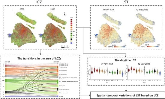
Exploring Spatiotemporal Variations in Land Surface Temperature Based on Local Climate Zones in Shanghai from 2008 to 2020

Abstract

Understanding changes in urban internal structure and land surface temperature (LST) is essential. The local climate zone (LCZ) scheme has been extensively applied to characterize urban spatial structure, which has potential for urban climate research. We combined optical imagery and synthetic aperture radar (SAR) data (Landsat-5 and PALSAR for 2008; Sentinel-2 and PALSAR-2 for 2020) to map the LCZs in Shanghai, China. The results showed that the areas of open high-rise and open mid-rise buildings significantly increased from 2008 to 2020. Then, we investigated the spatiotemporal variations in LST based on the LCZ data from 2008 to 2020 using the grid method. The mean daytime LST (obtained from Landsat-5 and Landsat-8) was higher in 2020 than in 2008 for each LCZ type in spring. The mean daytime LSTs of compact mid-rise, compact low-rise, large low-rise and heavy industry zones were higher than those of other LCZ types in spring and summer. The mean nighttime LST (obtained from ASTER) in the downtown area was higher than that in the suburbs in summer. Furthermore, the mean nighttime LST of the built types was also generally higher than that of the natural types in summer. A comparison of the mean daytime LSTs in 2008 and 2020 revealed that the expansion trend of the higher LST areas in spring and summer is consistent with the expansion areas of the mid-rise and high-rise built types.

1. Introduction

The local climate zone (LCZ) system has been broadly applied in urban surface thermal environments [1,2]. The LCZ scheme offers a universal classification for built types and natural types. Each LCZ class has a specific range of climate-relevant physical parameters [1]. The LCZ system can be easily applicable to most cities in the world and plays an increasingly important role for urban climate studies with respect to the thermal environment [3]. Currently, the data utilized for LCZ classification comprise mainly optical images from remote sensing data. Satellite images such as Landsat and Sentinel-2 are employed more frequently [4,5,6,7]. In addition, the use of synthetic aperture radar (SAR) data enables the extraction of additional urban land cover information [8]. The combination of multisource remote sensing data is the current trend associated with diverse LCZ classification methods [9]. The LCZ framework provides a good opportunity to link the urban climate and urban spatial structure, which can further quantify the association between the internal structure and the surface thermal environment. With the rapid growth of urbanization, the LCZ scheme has been applied to quantitative analysis studies on land surface temperature (LST). This approach resolves the issue of non-uniform classification in LST research studies [10]. Since the LCZ system further subdivides built types and natural types, a more detailed quantitative explore of the spatio-temporal characteristics of LST can be performed using the LCZ scheme. The measurement of urban LST is mainly based on remote sensing images from satellites and fixed-point observations of ground movements [11,12].

To close the standardization gap, the common concept of LCZs has risen as the top priority in surface urban heat island studies [13]. Over the past several years, an increasing number of studies have investigated the intricate relationship between LST and LCZ while also seeking to analyze the multifaceted effects of urbanization on LST [14,15]. Recent studies analyzed the surface urban heat islands for 50 cities, compared them using LCZs [10] and analyzed the growth season of plants and LCZs, which are also related to LSTs [16]. Other relevant studies have indicated that LST is negatively associated with vegetation cover [17], and LCZs show significant LST differences across seasons [18]. Likewise, researchers have also examined the spatial heterogeneity of LST for long time series and tested the statistical significance of LST differences in LCZs.

To benefit humankind, it is necessary to provide a better urban living environment. For the development of urban sustainability, it is important to advance and achieve the coordinated development of the regional population, resources, and environment. Focusing on cities, United Nations Sustainable Development Goal 11 is aimed at building healthy, safe, and sustainable cities. For Shanghai, most studies have examined how the population carrying capacity, urbanization trend, economic change, and PM2.5 influence the urban heat island effect [19,20,21,22]. However, few studies have focused on the spatiotemporal relationships between LCZs and LSTs in Shanghai. Changes in the density and height of buildings during urban development may affect their internal structures and LSTs. This study aims to fill the gap by using the LCZ classification system to analyze the LSTs in Shanghai.

The first objective of this study is to map the distribution of LSTs and LCZs to understand their spatial and temporal distribution characteristics. The second objective of this study is to connect the LCZ and LST distribution maps and to explore their relationship and the spatial and temporal distribution changes in LSTs over the past decade based on the LCZs.

2. Materials

2.1. Study Area

Shanghai is located at 30°40′–31°53′N and 120°51′–122°12′E (Figure 1). The northernmost part of Shanghai is the Chongming district, which is an island. In Shanghai, the terrain is flat, and the average altitude is approximately 4 m. Shanghai is densely distributed, with a dense water network. Many wetlands with abundant water resources are distributed in Shanghai. Moreover, Shanghai is one of the most important Chinese cities in terms of economic activity [21]. Since the 1990s, Shanghai has experienced rapid economic growth, urban land development, relocation, and deindustrialization, such as the Lujiazui area in Pudong [23,24].

2.2. Remote Sensing Data

We employed remote sensing data from Landsat-5 TM, PALSAR, Sentinel-2, and PALSAR-2 for LCZ classification (

Table 1. Data to be used in LCZ classification.

Satellite Data	Date	Band	Spatial Resolution (m)
Landsat-5 TM C1 Level-2	25 April 2008	Band 1–5, 7	30
ALOS PALSAR RTC	28 April 2008	HH, HV	20
	15 May 2008
	1 June 2008
Sentinel-2 MSI L2A	28 April 2020	Band 1–8, 8a, 9, 11, 12	10, 20, 60
ALOS-2 PALSAR-2 L3.1	2 May 2020 30 May 2020	HH, HV	10

).

To avoid the differences caused by different seasons, we selected images with less cloud cover in April, May, and June for LCZ classification. We selected data from Landsat-5 TM, Landsat-8, and Advanced Spaceborne Thermal Emission and Reflection Radiometer (ASTER) to generate LST maps for cloud-free conditions. Due to the inconsistent coverage and observation times of the sensors from different sources, the thermal data used for LST generation were selected to be close to the date of LCZ classification (

Table 2. Summary of remote sensing data used for LST mapping.

Scheme 8.	Date	Band	Spatial Resolution (m)	Time (GMT+8)
Landsat-5 TM C2 Level-1	25 April 2008	Band 3, 4, 6	30	10:14
	28 July 2007			10:18
	19 November 2008			10:08
	2 February 2007			10:20
Landsat-8 OLI/TIRS C2 Level-1	12 May 2020	Band 4, 5, 10	30	10:24
	16 August 2020			10:24
	22 December 2020			10:25
	22 February 2020			10:24
ASTER Level-2 AST_08	2 August 2019	—	90	22:07

Thermal bands (TIRS) in the Landsat series of satellite bands are registered to and delivered with the 30-meter data product.

). To ensure the consistency of the multisource remote sensing data, the image projection was unified as UTM_Zone_51N (WGS_1984).

The Landsat-5 Thematic Mapper (TM) C1 Level-2 data reflect the surface reflectance generated from Level-1 data. The Landsat-5 TM C2 Level-1 TIR product was improved with a precision correction algorithm to identify a good collection of correlated ground control points. The TIR band of Landsat-5 TM C2 Level-1 was used to retrieve the LST. The TIR band 10 of the Landsat-8 OLI/TIRS C2 Level-1 product was used to retrieve the LST. The Sentinel-2 multispectral instrument (MSI) Level-2A products from the European Space Agency (ESA) provide orthorectified, bottom-of-atmosphere reflectance with subpixel multispectral registration. The PALSAR series products used in this study were acquired in dual polarization in stripmap mode, including HH and HV bands. The ALOS PALSAR RTC products were processed with radiometric terrain correction and map projection. The ALOS-2 PALSAR-2 L3.1 product performs image quality correction, noise reduction, and dynamic range compression based on the L1.5 product. The ASTER Level-2 AST_08 products reflect the LST obtained from the ASTER data via the temperature and emissivity separation algorithm.

3. Methods

Figure 2 shows an overall flowchart that describes the main steps. The data preprocessing included resampling and normalization. We employed Landsat-5 TM and PALSAR data from 2008 and Sentinel-2 MSI and PALSAR data from 2020 to produce LCZ maps of Shanghai. We then produced LSTs using Landsat-5 TM data from 2008 and Landsat-8 OLI/TIRS data from 2020. We also used the ASTER product from 2019 to analyze the nighttime LST. The LCZ and LST in the same period were connected using the grid cell method.

3.1. LCZ Classification

We used a nearest neighbor interpolation method to resample the band spatial resolution to 10 m for processing. For 2008, the six spectral bands of Landsat-5 TM C1 Level-2 data were combined with the PALSAR bands. For 2020, the twelve spectral bands of the Sentinel-2 data were combined with the PALSAR-2 bands.

Considering LCZ types with similar characteristics in the study area, we combined LCZ 8 (large low-rise) and LCZ 10 (heavy industry) into LCZ 8&10. In addition, we also combined LCZ B (scattered trees) and LCZ C (bush and scrub) into LCZ B&C. The LCZ scheme in this study was composed of two types: built types (LCZs 1, 2, 3, 4, 5, 6, and 8&10) and natural types (LCZs A, B&C, D, E, F, and G). We collected ground truth samples of the 13 LCZ classes randomly based on visual interpretations from Google Earth. We randomly split the ground truth samples into training samples and test samples to ensure separation in their spatial distributions.

Table 3. The number of training and test pixels for images acquired in 2008 and 2020.

Class	Description	2008		2020
		Training	Test	Training	Test
LCZ 1	Compact high-rise	1264	241	4261	741
LCZ 2	Compact mid-rise	15,656	4873	3640	932
LCZ 3	Compact low-rise	53,494	14,445	11,180	4092
LCZ 4	Open high-rise	69,933	10,287	40,791	12,035
LCZ 5	Open mid-rise	211,189	70,466	59,962	19,785
LCZ 6	Open low-rise	114,805	25,423	22,547	7332
LCZ 8&10	Large low-rise and heavy industry	105,346	33,776	21,620	7700
LCZ A	Dense trees	3050	254	1463	1132
LCZ B&C	Scattered trees with bush and scrub	73,182	21,031	26,407	6134
LCZ D	Low plants	135,671	43,186	23,148	5051
LCZ E	Bare rock or paved	67,727	24,252	37,434	10,821
LCZ F	Bare soil or sand	41,915	9893	35,953	3978
LCZ G	Water	27,203	6088	23,349	4384
Total		920,435	264,215	311,755	84,117

shows the number of training and test pixels for each LCZ class.

In this study, we used random forest (RF) models to perform LCZ classification. RF classifiers are some of the most important models that employ certain subsets of training instances to construct multiple decision trees [25]. We trained different RF models using various combinations of the number of trees and the number of randomly selected features at each node. For the RF model, a grid search was performed, and the out-of-bag scores were used to determine the best combination. The number of trees was 1000 for both the 2008 and 2020 models. In addition, the numbers of features randomly selected at each node were four and eight for the 2008 and 2020 models, respectively.

3.2. LST Retrieval for Landsat-5 TM and Landsat-8

The Landsat-5 TM C2 Level-1 products for 2007–2008 and the Landsat-8 OLI/TIRS C2 Level-1 products for 2020 were used to retrieve the daytime LSTs. The radiation transfer equation is presented as follows [26]:

$${\mathrm{L}}_{\lambda }=[\epsilon \mathrm{B}({\mathrm{T}}_{\mathrm{s}})+(1-\epsilon ){\mathrm{L}}_{\mathrm{down}}]\cdot \tau +{\mathrm{L}}_{\mathrm{up}}$$

(1)

where ${\mathrm{L}}_{\lambda }$ is the radiance measured by the sensor, $\tau$ is the atmospheric transmittance, $\epsilon$ is the land surface emissivity, ${\mathrm{L}}_{\mathrm{u}\mathrm{p}}$ is the upwelling atmospheric radiance, ${\mathrm{L}}_{\mathrm{d}\mathrm{o}\mathrm{w}\mathrm{n}}$ is the downwelling atmospheric radiance, $\mathrm{B}({\mathrm{T}}_{\mathrm{s}})$ is the blackbody radiance provided by Planck’s law, and ${\mathrm{T}}_{\mathrm{s}}$ is the LST.

The land surface temperature was obtained using Planck’s formula [27]:

$${\mathrm{T}}_{\mathrm{s}}=\frac{{\mathrm{K}}_2}{\ln \left(\frac{{\mathrm{K}}_1}{\mathrm{B}({\mathrm{T}}_{\mathrm{s}})}+1\right)}$$

(2)

where ${\mathrm{K}}_1$ is calibration constant 1 and ${\mathrm{K}}_2$ is calibration constant 2; for Landsat-5 TM Band 6, ${\mathrm{K}}_1$ = 607.76 W·m⁻²·sr⁻¹·μm⁻¹ and ${\mathrm{K}}_2$ = 1260.56 K; for Landsat-8 TIRS Band 10, ${\mathrm{K}}_1$ = 774. 8853 W·m⁻²·sr⁻¹·μm⁻¹ and ${\mathrm{K}}_2$=1321. 0789 K.

The three types of surface emissivity ε were calculated as follows [28]:

$$\left\{\begin{array}{l}{\epsilon }_{\mathrm{water}}=0.995\\ {\epsilon }_{\mathrm{surface}}=0.9625+0.0614\mathrm{F}\mathrm{V}\mathrm{C}-0.0461\mathrm{F}\mathrm{V}{\mathrm{C}}^2\\ {\epsilon }_{\mathrm{building}}=0.9589+0.086\mathrm{F}\mathrm{V}\mathrm{C}-0.0671\mathrm{F}\mathrm{V}{\mathrm{C}}^2\end{array}\right.$$

(3)

where ${\epsilon }_{\mathrm{water}}$, ${\epsilon }_{\mathrm{surface}}$, and ${\epsilon }_{\mathrm{building}}$ are the surface specific emissivities of the water surface, natural surface, and urban area, respectively.

The fractional vegetation cover (FVC) was calculated as follows [29]:

$$\mathrm{F}\mathrm{V}\mathrm{C}=\frac{\mathrm{N}\mathrm{D}\mathrm{V}\mathrm{I}-\mathrm{N}\mathrm{D}\mathrm{V}{\mathrm{I}}_{\mathrm{Soil}}}{\mathrm{N}\mathrm{D}\mathrm{V}{\mathrm{I}}_{\mathrm{V}\mathrm{eg}}-\mathrm{N}\mathrm{D}\mathrm{V}{\mathrm{I}}_{\mathrm{Soil}}}$$

(4)

where NDVI is the normalized vegetation index, NDVI_Soil is the NDVI value of the completely bare soil coverage area, and NDVI_Veg is the NDVI value of the pixel completely covered by vegetation. The NDVI is expressed as follows:

$$\mathrm{N}\mathrm{D}\mathrm{V}\mathrm{I}=\frac{{\rho }_{\mathrm{N}\mathrm{I}\mathrm{R}}-{\rho }_{\mathrm{RED}}}{{\rho }_{\mathrm{N}\mathrm{I}\mathrm{R}}+{\rho }_{\mathrm{RED}}}$$

(5)

where ${\rho }_{\mathrm{N}\mathrm{I}\mathrm{R}}$ and ${\rho }_{\mathrm{RED}}$ stand for the surface reflectances acquired in the near-infrared and red (visible) bands, respectively.

3.3. Grid-Cell Processing

The advantage of using grid cells is that they enable the integration of various data into a grid of the same size [30]. In this study, the LCZ maps and the LST results were connected by the grid cells. First, we created 90 m × 90 m grid cells with unique IDs in ArcGIS 10.8. Next, the percentage of the area occupied by each LCZ class in each grid cell was calculated. We then assigned the LCZ category with the largest area percentage to each grid cell. Finally, we calculated the average LST in each grid cell for each period.

3.4. Moran′s I

To reveal the spatial autocorrelation, we used the global Moran′s I index [31] and the local Moran′s I index [32] with the daytime LSTs, expressed as:

$$I=\frac{n{\displaystyle \sum _{i=1}^n{\displaystyle \sum _{j=1}^n{\omega }_{\mathrm{ij}}\left(x_i-\overline{x}\right)\left(x_j-\overline{x}\right)}}}{\left({\displaystyle \sum _{i=1}^n{\displaystyle \sum _{j=1}^n{\omega }_{\mathrm{ij}}}}\right){\displaystyle \sum _{i=1}^n{\left(x_i-\overline{x}\right)}^2}}$$

(6)

where $n$ is the number of spatial units indexed by $i$ and $j$; $x_i$ and $x_j$ are the attributes for spatial units $i$ and $j$, respectively. $\overline{x}$ is the mean of the corresponding attribute, and ${\omega }_{\mathrm{ij}}$ is the spatial weight between spatial unit $i$ and $j$.

The local Moran′s I index is expressed as:

$$I_i=\frac{x_i-\overline{x}}{{\sigma }^2}{\displaystyle \sum _{j=1,j\ne i}^n\left[{\omega }_{\mathrm{ij}}\left(x_j-\overline{x}\right)\right]}$$

(7)

where ${\sigma }^2$ is the variance of the corresponding attribute of spatial units.

4. Results

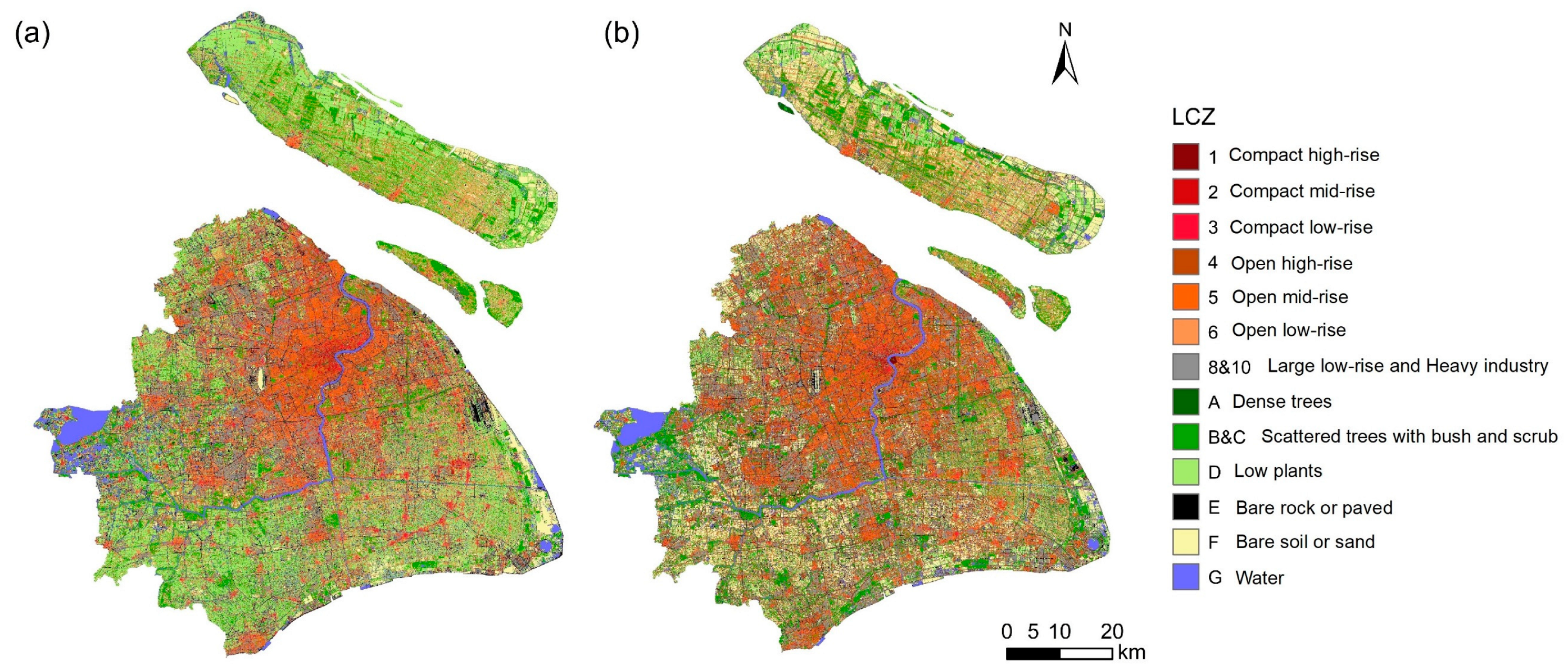
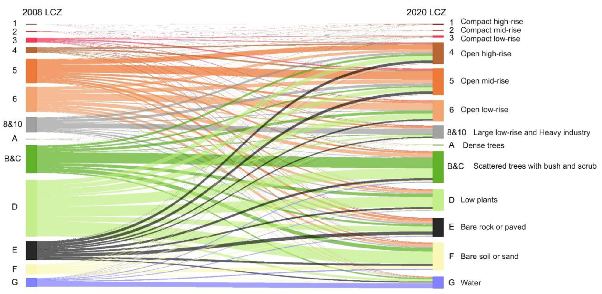
4.1. LCZ Mapping Results and Change Analysis

Figure 3 shows a comparison of the two phases of LCZ classification. The overall accuracy of the classification results for 2020 (80.40%) was higher than that for 2008 (75.35%). As expected, the accuracies of the LCZ classification results in both 2008 and 2020 were acceptable for change analysis.

Figure 4 illustrates the differences in the LCZ area percentages for 2008 and 2020. For both 2008 and 2020, LCZ 1 (Compact high-rise), LCZ 2 (Compact mid-rise), and LCZ A (dense trees) were much smaller in area than the other LCZ types. The area was considerably larger for open buildings (LCZs 4–6) than for compact buildings (LCZs 1–3).

In 2008, LCZ D (low plants) accounted for the largest area among all LCZ types (28.8%), followed by LCZ B&C (scattered trees with bush and scrub) (14.2%). Among the built types, LCZ 6 (open low-rise) had the largest area in 2008, followed by LCZ 5 (open mid-rise). LCZ 1, LCZ 2, and LCZ 4 (open high-rise) were mainly distributed in the central area of Shanghai. LCZ 3 (compact low-rise) was distributed in the central area and built-up areas in other districts, whereas LCZ 6 was mainly distributed in other districts of Shanghai. The area of LCZ 5 occupied a high proportion in the central city and its surrounding areas. LCZ 8&10 (large low-rise and heavy industry) and LCZ B&C were mainly evenly distributed in the noncentral area. LCZ A was rare in all districts of Shanghai. LCZ D was basically only distributed in noncentral urban areas. LCZ F (bare soil or sand) was sparsely scattered throughout Shanghai, with only a small portion in the eastern part of the city.

In 2020, LCZ B&C accounted for the largest area of all LCZ types (16.1%), followed by LCZ F (14.0%). Among the built types, LCZ 5 had the largest area in 2020, followed by LCZs 4 and 6. LCZ 1 was primarily concentrated in the central area (e.g., the Lujiazui area of the Pudong district), whereas LCZ 2 exhibited a more prominent distribution within the central area. LCZ 3 was evenly distributed throughout Shanghai, but the proportion was very small. LCZs 4 and 5 were distributed in various districts of Shanghai and were very dense and evenly distributed. LCZ 6 was densely distributed in the Chongming district and the south-central part of the Pudong district but was less and evenly distributed in other districts. LCZ 8&10 was distributed in every district, and its distribution was very concentrated. LCZ A was very small in area and was mainly distributed in Songjiang district. LCZs B&C and D were scattered in noncentral urban areas. LCZ F was densely distributed in the north, south, and west of Shanghai.

There were several major trends in the changes in the LCZ area percentages for the 2008–2020 period (Figure 4). From 2008 to 2020, LCZ 4 significantly increased from 2.7% to 11.0%, and LCZ F significantly increased from 5.0% to 14.0%. Conversely, from 2008 to 2020, LCZ D significantly decreased from 28.8% to 11.0%; LCZ 6 decreased from 13.0% to 10.7%; LCZ 3 decreased from 2.2% to 0.9%; and LCZ 8&10 decreased from 7.7% to 6.6%. The reason for the significant reduction in LCZ D is mainly attributed to rapid urbanization and changes in vegetation types, such as the conversion of LCZ D to LCZ B&C and F.

Figure 5 comprises two stacked vertical bars representing the LCZ types for 2008 and 2020 and one set of transition lines positioned between a pair of stacked bars. From 2008 to 2020, the expansion of LCZ 1 was primarily attributed to the transformation of LCZs 4, 5, and 8&10. The increase in LCZ 2 was mainly derived from LCZs 3, 5, and 8&10. The increase in LCZ 3 was mainly derived from LCZs 5, 6, and 8&10. The increase in LCZ 4 was mainly derived from LCZs 5, 6, D, and E. The increase in LCZ 5 was mainly derived from LCZs 6, 8&10, D, and E. The increase in LCZ 6 was mainly derived from LCZ 5, B&C and D. The increase in LCZ 8&10 was mainly derived from LCZs 5, D, and E. The increase in LCZ B&C was mainly derived from LCZs 6, D, and E. The increase in LCZ D was mainly derived from LCZs 6, B&C, and E. The increase in LCZ F was mainly derived from LCZs 6, B&C and D.

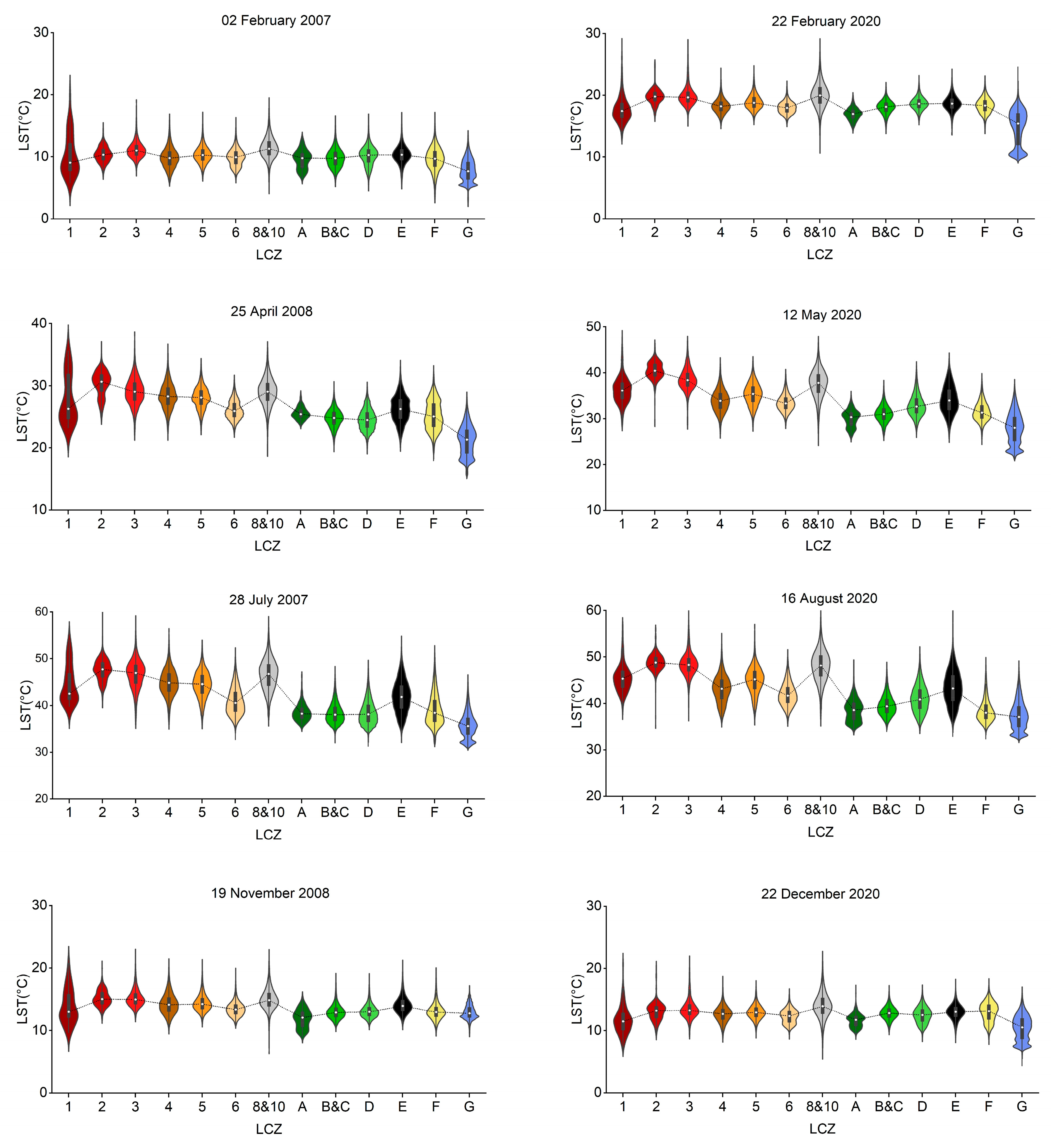
4.2. Relationships between Daytime LSTs and LCZs

Figure 6 displays the daytime LSTs for different dates in 2007 (hereafter, nominally 2008), 2008, and 2020. In the spring and summer, the areas with high daytime LSTs were distributed in the LCZ built types, and the daytime LSTs were relatively higher in the central area of Shanghai than in the suburbs. For 2008, the areas with high daytime LSTs were distributed mainly in the downtown area in the spring and summer. During the 2008–2020 period, the areas of high daytime LSTs in the spring and summer expanded from the central area to west of Shanghai. The daytime LSTs in both 2008 and 2020 were relatively high in northern Shanghai (except for Chongming district). The daytime LSTs in the Chongming district were low during the 2008–2020 period.

Figure 7 shows the local spatial autocorrelation of the daytime LSTs in 2008 and 2020. A significant strong positive spatial autocorrelation was observed in both spring and summer during the study period (

Table 4. Spatial autocorrelation results using the global Moran’s I statistic.

Date	Moran’s I	z Score	p Value
25 April 2008	0.895	2096.458	0.000
28 July 2007	0.888	2079.299	0.000
19 November 2008	0.784	1834.793	0.000
02 February 2007	0.804	1883.002	0.000
12 May 2020	0.887	2077.285	0.000
16 August 2020	0.897	2101.054	0.000
22 December 2020	0.818	1915.356	0.000
22 February 2020	0.820	1920.172	0.000

), revealing that the LST was strongly affected by spatial agglomeration with adjacent areas. In the spring and summer, the high–high clusters were mainly concentrated in the central area of Shanghai. These areas with high LSTs were covered by various built types. During the 2008–2020 period, the high–high clusters in spring and summer were expanded. The high–high clusters were mainly distributed in the northern area (except for the Chongming district) in November 2008, whereas the high–high clusters were mainly distributed in the southern area in December 2020. Low–high and high–low spatial outliers were rare in the whole study area for both 2008 and 2020.

Figure 8 shows the daytime LSTs corresponding to LCZ types using violin plots. Figure 9 shows the mean daytime LSTs of LCZ types for different months. Built LCZ types consistently exhibited higher mean daytime LSTs compared to natural LCZ types. The mean daytime LSTs of compact buildings and industrial plants were generally at high levels for most months. The mean daytime LSTs of LCZs A-D were lower than the built LCZ types in spring and summer. The daytime LST differences among LCZ types in the spring and summer were larger than those in the autumn and winter. The maximum LST difference among LCZ types in the summer exceeded 10 °C, while the LST difference among LCZ types in winter did not exceed 5 °C. The mean daytime LSTs of LCZs 2 and 3 were higher than those of LCZ 8&10 in the spring and summer, whereas the mean daytime LSTs of LCZ 8&10 in the autumn and winter were higher than those of all built types.

As shown in Figure 3, Figure 6 and Figure 8, for the daytime LSTs in 2008 and 2020, the expansion trend of the higher-LST areas in the spring and summer seasons was consistent with the expansion areas of the medium and high building types (e.g., LCZs 2, 3, and 8&10).

4.3. Relationships between Nighttime LSTs and LCZs

Figure 10 shows the nighttime LST map in part of Shanghai at a 90 m resolution and a violin plot of the nighttime LSTs of LCZ types in 2019. The contrast between the city center and the suburbs for Shanghai′s nighttime LST is significant, and the nighttime LST of the city center was significantly higher than that of the suburbs. The areas with higher nighttime LSTs were mainly concentrated in areas with LCZ G, LCZ E, and compact buildings.

The mean nighttime LSTs of natural LCZ types (except for LCZs G and E) were typically lower than those of built LCZ types. The overall LST difference at night was smaller than during the day. The mean nighttime LSTs of compact buildings were generally higher than those of open buildings, and the mean nighttime LSTs of mid-rise and high-rise buildings were higher than those of low-rise buildings. Among the built LCZ types, the mean nighttime LST of LCZ 1 was the highest, whereas the mean nighttime LST of LCZ 6 was the lowest. Among the natural LCZ types, the mean nighttime LSTs were relatively high for LCZs E and G, whereas the mean nighttime LST of LCZ D was the lowest.

5. Discussion

A comparison of the LCZ maps for 2008 and 2020 (Figure 3) showed that the shift among built types was mainly observed in the shift from LCZ 3, 5, and 6 to LCZ 4, which may be related to the renovation of old urban residential areas and the expansion of urban built-up areas [21]. The increase in the area of LCZ 1 (compact high-rise) may be attributed to the government′s construction and development of the Pudong district, such as the Lujiazui area [33]. Additionally, the area percentage of LCZ D (low plants) was significantly reduced (Figure 4). This reduction may be attributed to population growth putting pressure on the infrastructure in cities [34]. The area of scattered trees with bush and scrub (LCZ B&C) demonstrated an increase, likely due to the implementation of policies that provide opportunities for afforestation [35].

According to Figure 11, during the summer, the mean daytime LST differences above 5 °C were concentrated between built and natural types. This discovery was consistent with other studies [36], which also indicated that the LST significantly changes with built types. Notably, in the LST comparison between the built types and the other LCZ types, LCZs 2 (compact mid-rise), 3 (compact low-rise), and 8&10 (large low-rise and heavy industry) were the most evident. Although the area of LCZ 2 was relatively small, it significantly contributed to the LST difference, even more so than the compact high-rise (LCZ 1).

We further explored the mean daytime LST differences between each LCZ type and LCZ D (low plants) (Figure 12). As shown in Figure 12, the mean daytime LST differences between the built types and LCZ D were positive in the spring and summer. Among different seasons, there was a considerable variation in mean daytime LST differences between the built types and LCZ D. Similar phenomena have been found in previous studies [10]. As shown in Figure 11 and Figure 12, the positive and large differences in the mean daytime LSTs between LCZ E and the other natural types were observed, which may be due to the thermal properties of materials, high levels of human activity, and the highly developed traffic in Shanghai during the daytime. Surprisingly, in terms of the mean daytime LST differences between the built and natural types, LCZ 1 was comparatively lower than LCZs 2 and 3, which may be due to shadows and aerodynamic differences.

Figure 8 and Figure 9 reveal that the mean daytime LST was higher for built types than for natural types in summer, which was consistent with the previous research findings [14,37,38]. The results indicated that the LST significantly changed with built types. During the summer, LCZs 1 and 4 presented a relatively low mean daytime LST but a relatively high mean nighttime LST. This difference may be attributed to the shading effects of buildings during the daytime and the significant number of vertical surfaces that may potentially impact the mean daytime LST [13]. The collective thermal properties of materials could vary among the various types of building structures [39,40]. Most of LCZ 1 is in the Lujiazui area, which is close to the Huangpu River. Therefore, in addition to heat storage release, LCZ 1 is probably influenced by the surrounding water bodies, resulting in a slow temperature drop at night.

Among the built types, LCZ 8&10 had almost the highest mean daytime and nighttime LSTs in the built types, which was consistent with previous studies [41]. Note that the mean daytime LSTs of LCZ 8&10 in all seasons were relatively high, which may be attributed to the acceleration of industrialization. The numerous impervious surfaces lead to high albedo in industrial areas, where heat may be emitted and accumulated. The mean nighttime LSTs of LCZ 8&10 also reached relatively high levels, perhaps because shift work patterns were implemented by factories.

During the study period, urban expansion in Shanghai resulted in the loss of LCZ D (low plants) (Figure 5). Most of LCZ D was converted into scattered trees with bush and scrub (LCZ B&C), bare soil or sand (LCZ F), and various built types. Of these types, LCZ B&C (such as street trees, parks, and sidewalk trees) may have a better cooling effect than impervious surfaces [42]. Note that LCZ F accounts for 14.0% of the land in Shanghai, with an area increase of 9.0% from 2008 to 2020 (Figure 4), indicating that undeveloped areas account for a large proportion, which may indicate the transition from natural to urban environments. This finding reflects the need to pay attention to the LST during urban development, since the mean LST of LCZ F almost reaches 40 °C during the daytime in the summer.

6. Conclusions

We combined optical images and SAR data to map the LCZs from 2008 to 2020. Quantitative analyses of the LCZs and LSTs revealed that the changes in the internal urban structure of Shanghai lead to changes in the LST. From 2008 to 2020, the increase in open high-rise buildings was mainly transformed from mid-rise and low-rise buildings. The transformation of low plants (LCZ D) to open high-rise, open mid-rise, and open low-rise buildings (LCZ 4, 5, and 6) in Shanghai began in the late 1990s and early 2000s.

During the study period, the number of compact high-rise and compact mid-rise buildings expanded from a small part of the Lujiazui area to the entire Lujiazui area and the central city area, mainly at the expense of green space (e.g., LCZ D) and renovation based on old residential areas. From 2008 and 2020, the number of open high-rise buildings substantially increased in the central city. As the built LCZs increased, the mean daytime LST for each built LCZ type also tended to increase. Among the built LCZ types, large low-rise and heavy industry (LCZ 8&10) types had high mean daytime and nighttime LSTs in both 2008 and 2020.

The spatiotemporal analysis using grid cells demonstrated that the dispersion of areas with high LSTs and the proliferation of regions experiencing rising LSTs in Shanghai varied significantly among different LCZ categories. Additionally, the methodology presented in this study shows promising potential for application in other urban environments. Specifically, combining optical and SAR data offers a detailed understanding of land cover and land use dynamics based on the LCZ system in urban areas. Moreover, employing grid cells to connect LCZ and LST data enables a more precise evaluation of the spatiotemporal patterns of LST across LCZs. Lastly, it is worth noting that the replication of this approach in other cities requires careful considerations of data availability, local urban structures, and calibration to suit local conditions. This approach can be adapted and validated for diverse contexts, and it is pivotal for researchers and urban planners to critically assess its applicability based on specific urban characteristics.

References

1. Stewart, I.D.; Oke, T.R. Local Climate Zones for Urban Temperature Studies. Bull. Am. Meteorol. Soc. 2012, 93, 1879–1900. [Google Scholar] [CrossRef]
2. Middel, A.; Nazarian, N.; Demuzere, M.; Bechtel, B. Urban Climate Informatics: An Emerging Research Field. Front. Environ. Sci. 2022, 10, 867434. [Google Scholar] [CrossRef]
3. Aslam, A.; Rana, I.A. The use of local climate zones in the urban environment: A systematic review of data sources, methods, and themes. Urban Clim. 2022, 42, 101120. [Google Scholar] [CrossRef]
4. Huang, X.; Liu, A.; Li, J. Mapping and analyzing the local climate zones in China’s 32 major cities using Landsat imagery based on a novel convolutional neural network. Geo-Spat. Inf. Sci. 2021, 24, 528–557. [Google Scholar] [CrossRef]
5. Demuzere, M.; Kittner, J.; Martilli, A.; Mills, G.; Moede, C.; Stewart, I.D.; Vliet, J.V.; Bechtel, B. A global map of local climate zones to support earth system modelling and urban-scale environmental science. Earth Syst. Sci. Data 2022, 14, 3835–3873. [Google Scholar] [CrossRef]
6. Ren, J.; Yang, J.; Zhang, Y.; Xiao, X.; Xia, J.C.; Li, X.; Wang, S. Exploring thermal comfort of urban buildings based on local climate zones. J. Clean. Prod. 2022, 340, 130744. [Google Scholar] [CrossRef]
7. Shi, Z.; Yang, J.; Zhang, Y.; Xiao, X.; Xia, J.C. Urban ventilation corridors and spatiotemporal divergence patterns of urban heat island intensity: A local climate zone perspective. Environ. Sci. Pollut. Res. 2022, 29, 74394–74406. [Google Scholar] [CrossRef]
8. Zhu, Z.; Woodcock, C.E.; Rogan, J.; Kellndorfer, J. Assessment of spectral, polarimetric, temporal, and spatial dimensions for urban and peri-urban land cover classification using Landsat and SAR data. Remote Sens. Environ. 2012, 117, 72–82. [Google Scholar] [CrossRef]
9. La, Y.; Bagan, H.; Yamagata, Y. Urban land cover mapping under the Local Climate Zone scheme using Sentinel-2 and PALSAR-2 data. Urban Clim. 2020, 33, 100661. [Google Scholar] [CrossRef]
10. Bechtel, B.; Demuzere, M.; Mills, G.; Zhan, W.; Sismanidis, P.; Small, C.; Voogt, J. SUHI analysis using Local Climate Zones—A comparison of 50 cities. Urban Clim. 2019, 28, 100451. [Google Scholar] [CrossRef]
11. Yan, C.; Guo, Q.; Li, H.; Li, L.; Qiu, G.Y. Quantifying the cooling effect of urban vegetation by mobile traverse method: A local-scale urban heat island study in a subtropical megacity. Build. Environ. 2020, 169, 106541. [Google Scholar] [CrossRef]
12. Chen, C.; Bagan, H.; Xie, X.; La, Y.; Yamagata, Y. Combination of Sentinel-2 and PALSAR-2 for Local Climate Zone Classification: A Case Study of Nanchang, China. Remote Sens. 2021, 13, 1902. [Google Scholar] [CrossRef]
13. Cilek, M.U.; Cilek, A. Analyses of land surface temperature (LST) variability among local climate zones (LCZs) comparing Landsat-8 and ENVI-met model data. Sustain. Cities Soc. 2021, 69, 102877. [Google Scholar] [CrossRef]
14. Badaro-Saliba, N.; Adjizian-Gerard, J.; Zaarour, R.; Najjar, G. LCZ scheme for assessing Urban Heat Island intensity in a complex urban area (Beirut, Lebanon). Urban Clim. 2021, 37, 100846. [Google Scholar] [CrossRef]
15. Huang, F.; Jiang, S.; Zhan, W.; Bechtel, B.; Liu, Z.; Demuzere, M.; Huang, Y.; Xu, Y.; Ma, L.; Xia, W.; et al. Mapping local climate zones for cities: A large review. Remote Sens. Environ. 2023, 292, 113573. [Google Scholar] [CrossRef]
16. Kabano, P.; Lindley, S.; Harris, A. Evidence of urban heat island impacts on the vegetation growing season length in a tropical city. Landsc. Urban Plan. 2021, 206, 103989. [Google Scholar] [CrossRef]
17. Aslam, A.; Rana, I.A.; Bhatti, S.S. The spatiotemporal dynamics of urbanisation and local climate: A case study of Islamabad, Pakistan. Environ. Impact Assess. Rev. 2021, 91, 106666. [Google Scholar] [CrossRef]
18. Li, X.; Stringer, L.C.; Dallimer, M. The role of blue green infrastructure in the urban thermal environment across seasons and local climate zones in East Africa. Sustain. Cities Soc. 2022, 80, 103798. [Google Scholar] [CrossRef]
19. Cui, L.; Shi, J. Urbanization and its environmental effects in Shanghai, China. Urban Clim. 2012, 2, 1–15. [Google Scholar] [CrossRef] [Green Version]
20. Li, C.; Shen, D.; Dong, J.; Yin, J.; Zhao, J.; Xue, D. Monitoring of urban heat island in Shanghai, China, from 1981 to 2010 with satellite data. Arab. J. Geosci. 2014, 7, 3961–3971. [Google Scholar] [CrossRef]
21. Yue, W.; Fan, P.; Wei, Y.D.; Qi, J. Economic development, urban expansion, and sustainable development in Shanghai. Stoch. Environ. Res. Risk Assess. 2014, 28, 783–799. [Google Scholar] [CrossRef]
22. Miao, Y.; Che, H.; Zhang, X.; Liu, S. Relationship between summertime concurring PM2.5 and O3 pollution and boundary layer height differs between Beijing and Shanghai, China. Environ. Pollut. 2021, 268, 115775. [Google Scholar] [CrossRef]
23. Walcott, S.M.; Pannell, C.W. Metropolitan spatial dynamics: Shanghai. Habitat Int. 2006, 30, 199–211. [Google Scholar] [CrossRef] [Green Version]
24. Frazier, M.W. The Power of Place Contentious Politics in Twentieth-Century Shanghai and Bombay, 1st ed.; Cambridge University Press: Cambridge, UK, 2019; pp. 1–26. [Google Scholar] [CrossRef]
25. Belgiu, M.; Drăguţ, L. Random forest in remote sensing: A review of applications and future directions. Remote Sens. Environ. 2016, 114, 24–31. [Google Scholar] [CrossRef]
26. Sobrino, J.; Jiménez-Muñoza, J.C.; Paolini, L. Land surface temperature retrieval from LANDSAT TM 5. Remote Sens. Environ. 2004, 90, 434–440. [Google Scholar] [CrossRef]
27. Chander, G.; Markham, B. Revised Landsat-5 TM radiometric calibration procedures and postcalibration dynamic ranges. IEEE Trans. Geosci. Remote Sens. 2003, 41, 2674–2677. [Google Scholar] [CrossRef] [Green Version]
28. Qin, Z.H.; Li, W.J.; Xu, B.; Chen, Z.X.; Liu, J. The estimation of land surface emissivity for Landsat TM6. Remote Sens. Land Res. 2004, 16, 28–32, 36, 41. (In Chinese) [Google Scholar] [CrossRef]
29. Gao, L.; Wang, X.; Johnson, B.A.; Tian, Q.; Wang, Y.; Verrelst, J.; Mu, X.; Gu, X. Remote sensing algorithms for estimation of fractional vegetation cover using pure vegetation index values: A review. ISPRS J. Photogramm. Remote Sens. 2020, 159, 364–377. [Google Scholar] [CrossRef]
30. Bagan, H.; Yamagata, Y. Analysis of urban growth and estimating population density using satellite images of nighttime lights and land-use and population data. GIScience Remote Sens. 2015, 52, 765–780. [Google Scholar] [CrossRef]
31. Getis, A.; Ord, J.K. The analysis of spatial association by use of distance statistics. Geog. Anal. 1992, 24, 189–206. [Google Scholar] [CrossRef]
32. Anselin, L. Local indicators of spatial association—LISA. Geogr. Anal. 1995, 27, 93–115. [Google Scholar] [CrossRef]
33. Xue, C.Q.L.; Zhai, H.; Mitchenere, B. Shaping Lujiazui: The formation and building of the CBD in Pudong, Shanghai. J. Urban Des. 2011, 16, 209–232. [Google Scholar] [CrossRef]
34. Byomkesh, T.; Nakagoshi, N.; Dewan, A.M. Urbanization and green space dynamics in Greater Dhaka, Bangladesh. Landsc. Ecol. Eng. 2012, 8, 45–58. [Google Scholar] [CrossRef]
35. Du, H.; Cai, Y.; Zhou, F.; Jiang, H.; Jiang, W.; Xu, Y. Urban blue-green space planning based on thermal environment simulation: A case study of Shanghai, China. Ecol. Indic. 2019, 106, 105501. [Google Scholar] [CrossRef]
36. Yang, J.; Ren, J.; Sun, D.; Xiao, X.; Xia, J.; Jin, C.; Li, X. Understanding land surface temperature impact factors based on local climate zones. Sustain. Cities Soc. 2021, 69, 102818. [Google Scholar] [CrossRef]
37. Ochola, E.M.; Fakharizadehshirazi, E.; Adimo, A.O.; Mukundi, J.B.; Wesonga, J.M.; Sodoudi, S. Inter-local climate zone differentiation of land surface temperatures for management of urban heat in Nairobi City, Kenya. Urban Clim. 2020, 31, 100540. [Google Scholar] [CrossRef]
38. Choudhury, D.; Das, A.; Das, M. Investigating thermal behavior pattern (TBP) of local climatic zones (LCZs): A study on industrial cities of Asansol-Durgapur development area (ADDA), eastern India. Urban Clim. 2021, 35, 100727. [Google Scholar] [CrossRef]
39. Chen, C.; Bagan, H.; Yoshida, T.; Borjigin, H.; Gao, J. Quantitative analysis of the building-level relationship between building form and land surface temperature using airborne LiDAR and thermal infrared data. Urban Clim. 2022, 45, 101248. [Google Scholar] [CrossRef]
40. Chen, C.; Bagan, H.; Yoshida, T. Multiscale mapping of local climate zones in Tokyo using airborne LiDAR data, GIS vectors, and Sentinel-2 imagery. GIScience Remote Sens. 2023, 60, 2209970. [Google Scholar] [CrossRef]
41. Khoshnoodmotlagh, S.; Daneshi, A.; Gharari, S.; Verrelst, J.; Mirzaei, M.; Omranie, H. Urban morphology detection and it’s linking with land surface temperature: A case study for Tehran Metropolis, Iran. Sustain. Cities Soc. 2021, 74, 103228. [Google Scholar] [CrossRef]
42. Aram, F.A.; García, E.H.; Solgi, E.; Mansournia, S. Urban green space cooling effect in cities. Heliyon 2019, 5, e01339. [Google Scholar] [CrossRef] [PubMed] [Green Version]
Figure 1. The green polygon indicates the boundary of the study area. The red rectangle is the area of the ASTER image.
Remotesensing 15 03106 g001
Figure 2. Workflow of LCZ mapping and analysis of LST approaches.
Remotesensing 15 03106 g002
Figure 3. LCZ classification maps in Shanghai for (a) 2008 and (b) 2020 at a resolution of 10 m.
Remotesensing 15 03106 g003
Figure 4. Percentages of the area covered by each LCZ in 2008 and 2020.
Remotesensing 15 03106 g004
Figure 5. Sankey diagram demonstrating the transitions in the LCZs from 2008 to 2020. The width of the lines is proportional to the quantity of flow. The left side shows the outflow in 2008, and the right side shows the inflow in 2020.
Remotesensing 15 03106 g005
Figure 6. Daytime LSTs in Shanghai on different dates (Table 2 provides a description of the dates) at 30 m resolution.
Remotesensing 15 03106 g006
Figure 7. Maps of significant hot spots, cold spots, and spatial outliers for the daytime LSTs using the local Moran’s I statistic.
Remotesensing 15 03106 g007
Figure 8. Violin plots of the daytime LSTs for each LCZ type for different months in 2007, 2008, and 2020.
Remotesensing 15 03106 g008
Figure 9. Mean daytime LSTs in each LCZ type for different months in 2007, 2008, and 2020.
Remotesensing 15 03106 g009
Figure 10. (a) Nighttime LST map from the ASTER LST product in Shanghai. (b) Violin plot of the nighttime LSTs for each LCZ type in 2019.
Remotesensing 15 03106 g010
Figure 11. Mean daytime LST differences (°C) between pairs of LCZ types in summer for (a) 2007 and (b) 2020 (ΔT = horizontal axis minus vertical axis).
Remotesensing 15 03106 g011
Figure 12. Mean daytime LST difference (°C) in LCZ types compared to LCZ D (low plants) in all dates.
Remotesensing 15 03106 g012