Article

AM–GM Algorithm for Evaluating, Analyzing, and Correcting the Spatial Scaling Bias of the Leaf Area Index

1
State Key Laboratory of Remote Sensing Science, Faculty of Geographical Science, Beijing Normal University, Beijing 100875, China
2
Beijing Engineering Research Center for Global Land Remote Sensing Products, Faculty of Geographical Science, Beijing Normal University, Beijing 100875, China
3
Faculty of Arts and Sciences, Beijing Normal University, Zhuhai 519087, China
*
Author to whom correspondence should be addressed.
Remote Sens. 2023, 15(12), 3068; https://doi.org/10.3390/rs15123068
Submission received: 24 April 2023 / Revised: 27 May 2023 / Accepted: 8 June 2023 / Published: 12 June 2023

Abstract

:
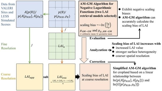
The leaf area index (LAI) is a crucial variable in climate, ecological, and land surface modeling. However, the estimation of the LAI from coarse-resolution remote sensing data can be affected by the spatial scaling bias, which arises from the nonlinearity of retrieval models and the heterogeneity of the land surface. This study provides an algorithm named Arithmetic Mean and Geometric Mean (AM–GM) to correct the spatial scaling bias. It is established based on negative logarithmic functions and avoids second-order stationarity. In this algorithm, relationships are derived between the scaling bias of LAI and the arithmetic and geometric means of directional gap probability for two commonly used remote sensing models, the Beer–Lambert law and a semi-empirical transfer function, respectively. According to the AM–GM algorithm, the expression representing the model nonlinearity is derived and utilized for the analysis of LAI scaling bias. Furthermore, the AM–GM algorithm is simplified by a linear relationship, which is constructed between two quantities related to the directional gap probability between two specific resolutions. Two scenes simulated by the LargE-Scale remote sensing data and image Simulation framework (LESS) model and three sites are used to evaluate the proposed algorithm and analyze the scaling bias of LAI. The validation results show that the AM–GM algorithm provides accurate correction of LAI scaling bias. The analyses based on the AM–GM algorithm demonstrate that the scaling bias of LAI increases with the increase in the LAI value, with stronger surface heterogeneity and coarser spatial resolution. The validation results of the simplified AM–GM algorithm demonstrate that at the Sud-Ouest site, the absolute value of the bias for the estimated LAI decreases from 0.10, 0.22, 0.29, and 0.31 to 0.04, 0.01, 0.04, and 0.05 at 200 m, 500 m, 1000 m, and 1500 m resolutions, respectively. In conclusion, the proposed algorithm is effective in the analysis and correction of the scaling bias for coarse-resolution LAI.

Graphical Abstract

1. Introduction

The leaf area index (LAI) is an essential variable in ecological, land surface, and climate modeling, as it explains the transfer of water, carbon, and energy between vegetation and the atmosphere [1,2]. The LAI is defined as one-half of the total green leaf area per unit of horizontal ground surface area [3]. In recent years, much research has applied coarse-resolution LAI (250 m–1000 m) to comprehend global vegetation change [4,5] and ecosystem productivity [6,7]. However, the accurate estimation of LAI at coarse resolution using remote sensing methods has been challenging due to the scaling effect [8].
The scaling effect is caused by model nonlinearity and surface heterogeneity. Most retrieval functions are nonlinear and built at a local scale (fine resolution) [9,10], which only interprets the surface heterogeneity at the corresponding scale [11,12]. When these functions are applied to a coarse spatial resolution, the scaling effect causes spatial scaling bias of LAI estimation [13,14]. Yin et al. reported that the scaling bias in LAI inversion can reach up to 26% [15]. Hence, scaling bias is an important consideration for the LAI estimated from coarse-resolution remote sensing data, especially on a heterogeneous surface [16,17,18].
To deal with this task, previous studies have proposed several methods. On the one hand, statistical regression relationships have been developed to calculate the spatial scaling bias [19,20]. For example, Zhao and Fan established a statistical regression relationship between a spatial heterogeneity coefficient and the scaling bias of LAI. However, empirical methods require external factors that limit their applicability. On the other hand, a series of universal methods have been provided [8,21,22,23,24,25,26]. For instance, the computational geometry method (CGM) sets the upper and lower envelopes of the retrieval model to achieve accurate parameter estimation at coarse resolutions [21]. The advantage of this method is that it is not affected by the continuity of the remote sensing model and does not require high-resolution remote sensing data. However, the true distribution of parameters is not considered. Chen et al. addressed the limitations of the CGM algorithm by introducing variable weights instead of fixed weights [26]. Nevertheless, the inherent flaw of the CGM method—its inability to express the scaling bias using a formula—has yet to be resolved. Similarly, machine learning models estimated parameters at coarse resolution based on the relationships built at a fine resolution, and the accuracy of the inversion parameter was controlled by the reference parameters at a coarse resolution [27]. Such methods are not suitable for analyzing scaling bias because a relevant formula cannot be established. The Taylor series expansion method (TSEM) is another universal method in which each term has a physical meaning [22]. This method is helpful for analyzing scaling bias. However, the arithmetic mean of the input variable for the LAI retrieval models is used to derive the second derivative term in the TSEM, which also ignores the true distribution of parameters [10,28]. This method also requires synchronous fine-resolution remote sensing data. Later, Garrigues et al. extended the TSEM algorithm to a multivariate transfer function but still left the problem unresolved [8]. Recently, several upscaling models are proposed based on fractal theory [23,24,25]. A number of studies have attempted to explain the fractal dimension [29], but no consensus has been reached. In summation, the TSEM algorithm is more suitable for analyzing and correcting the scaling bias, but the algorithm itself is limited by second-order stationarity and fine-resolution data.
TSEM is closely related to the model type [30]. In mathematics, scaling bias is referred to as negative Holder’s defect. When the model form is a negative logarithmic function, Holder’s defect can be accurately expressed by utilizing the arithmetic and geometric means of the input variables [31]. Hence, the negative logarithmic functions can be employed to develop a method for calculating and correcting the scaling bias. Two commonly used LAI inversion models with negative logarithmic form, the Beer–Lambert law [32] and a semi-empirical transfer function that establishes the relationship between the normalized difference vegetation index (NDVI) to LAI [33], are employed in this research. Notably, the equation for NDVI related to reflectance is nonlinear, leading to the scaling bias of NDVI on heterogeneous surfaces [8,34]. This bias not only affects the scaling bias calculation but also hinders the analysis of the scaling bias and the comprehensive understanding of the scaling effect.
In this study, an Arithmetic Mean and Geometric Mean (AM–GM) algorithm is proposed to deeply analyze and correct the LAI scaling bias. The algorithm aims to solve the inherent flaws of the TSEM. The practicality of this algorithm is enhanced by establishing a linear relationship between two specific resolutions, eliminating the need for fine-resolution remote sensing data.

2. Materials

In this study, data are obtained from both simulated scenes and in situ sites to validate the algorithm and analyze the scaling bias of LAI. The LargE-Scale remote sensing data and image Simulation framework (LESS) model were employed to simulate heterogeneous 3D scenes [35]. The in situ data were downloaded from the VAlidation of Land European Remote-sensing Instruments (VALERI) project (http://w3.avignon.inra.fr/valeri/, accessed on 15 March 2023). Two simulated scenes and three in situ sites are used to analyze and validate the proposed algorithm, and the land cover type includes cropland and forest. Four additional cropland sites are selected to simplify the AM–GM algorithm. At simulated scenes, the data are simulated at 1 m and then aggregated to 5 m, 9 m, 15 m, and 45 m. At the VALERI sites, the data are obtained at 20 m spatial resolution and aggregated to 200 m, 500 m, 1000 m, 1500 m, and 3000 m.

2.1. Simulated Data

Two 3D forest scenes are constructed using the LESS model in this paper, as shown in Figure 1. Both scenes have an area of 45 m × 45 m. The first scene consists of 581 trees. These trees are derived from 42 single-tree models, simulated by 6 different canopy shapes and 7 levels of leaf area index. Each tree’s position is determined based on field measurements. The LAI of the whole scene is 2.67. For more detailed information on the scene construction, please refer to Scene S4, which was constructed by Xu et al. [36]. Additionally, a virtual forest scene with stronger surface heterogeneity is constructed from the same single-tree models and different numbers of trees. The LAI of this virtual scene is 2.14. The spectral information of leaves and soil has been measured on the ground by Xu et al. [36]. The data simulations are performed with an observation zenith angle of 0°. Detailed parameter settings can be found in Table 1.
Over the simulated scenes, the directional gap probabilities are calculated from four component products, which are simulated using the LESS model:
p θ = p i s + p s s
where p i s and p s s represent the proportions of illuminated soil and shaded soil within each pixel, respectively. At a spatial resolution of 1 m, the directional gap probabilities are simulated. The results are then aggregated to coarser spatial resolutions of 5 m, 9 m, 15 m, and 45 m.

2.2. Site Data

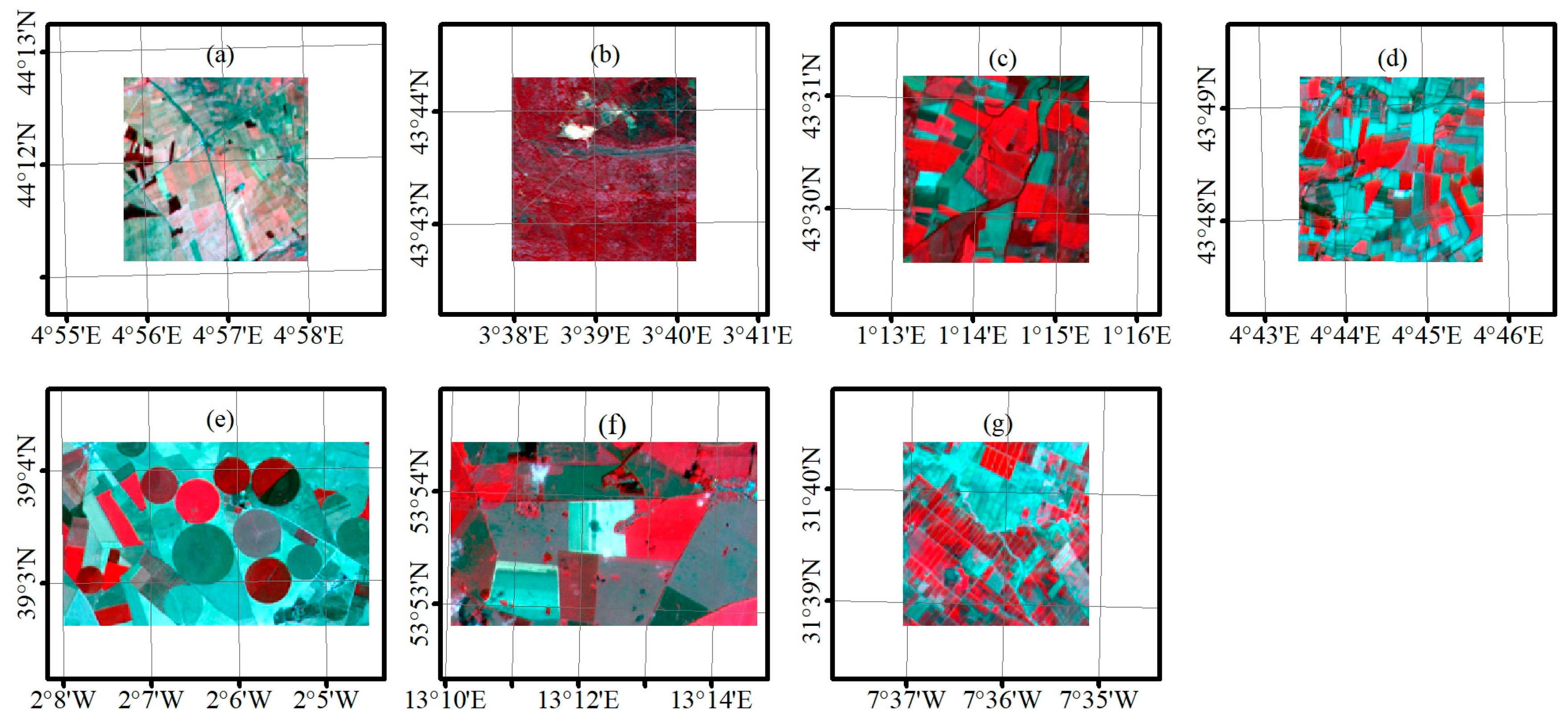
Seven VALERI sites are used and the data of these sites are downloaded from the VALERI website (Figure 2). To validate the algorithm and analyze the scaling bias, three sites are used. In particular, the vineyard dominates the Plan-de-Dieu site; Quercus ilex dominates the Puéchabon site; and the Sud-Ouest site includes nine crops, including corn, soya, sunflower, harvest wheat, etc. To simplify the AM–GM algorithm, four additional cropland sites covered by a variety of crops are chosen, including Les Alpilles, Barrax, Demmin, and Haouz. Table 2 provides detailed information about these sites, including land cover, image acquisition time, site size, and location.
Near-infrared ( ρ N I R ) and red ( ρ R ) reflectances are obtained from SPOT images, which have a spatial resolution of 20 m. These data are aggregated to coarser resolutions (200 m, 500 m, 1000 m, 1500 m, and 3000 m), then NDVI and directional gap probability are computed at those spatial resolutions. The in situ LAI data are also downloaded to build the retrieval model at 20 m spatial resolution.

3. Methods

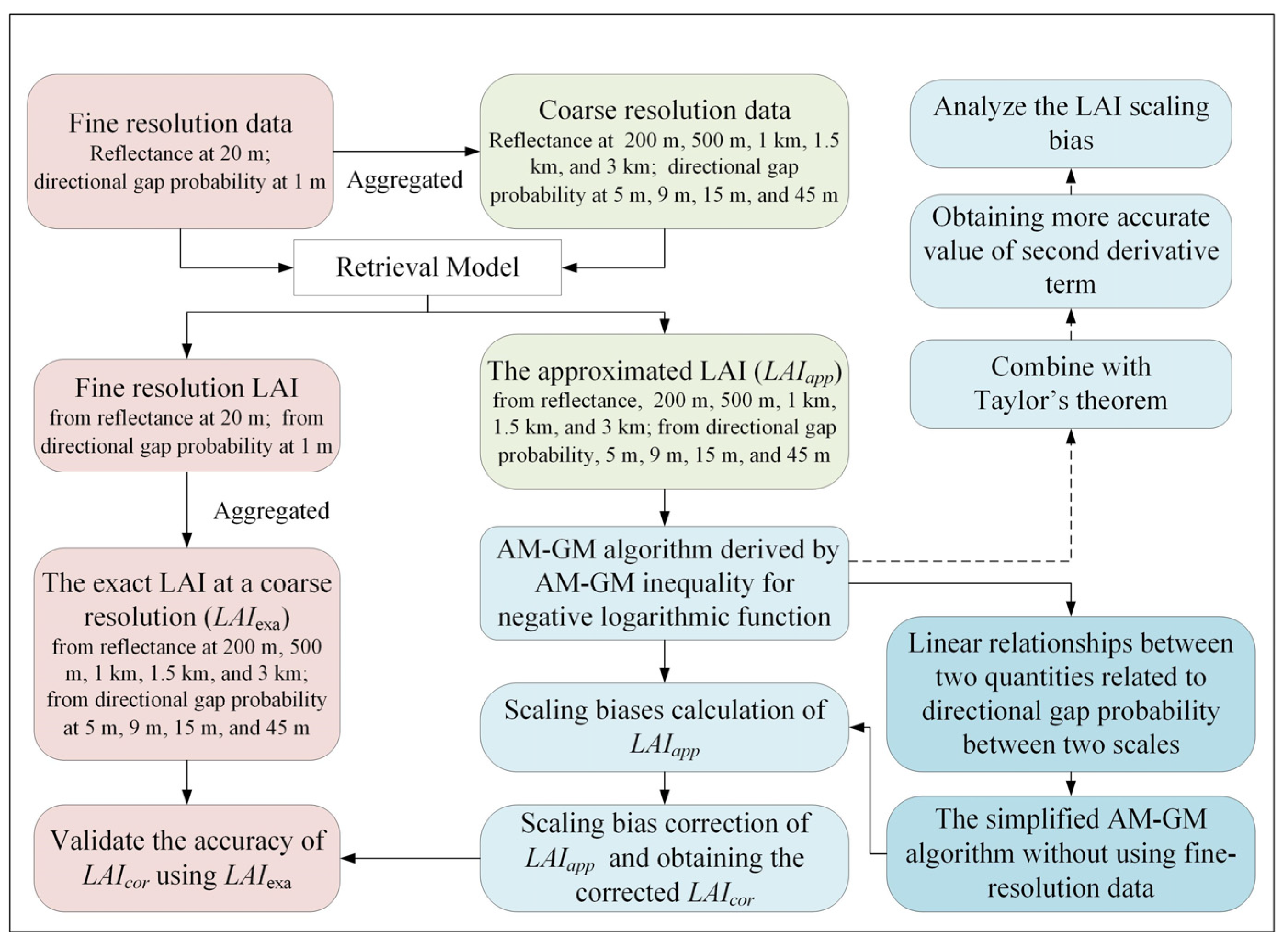
In this study, a novel algorithm called AM–GM is proposed to more accurately evaluate, analyze, and correct the scaling bias of LAI. This algorithm utilizes the advantage of negative logarithmic functions to avoid the second-order stationarity hypothesis, and this algorithm considers the scaling bias of NDVI. Moreover, the practicality of this algorithm is improved by eliminating the requirement for fine-resolution remote sensing data. In particular, the relationship between the LAI scaling bias and the arithmetic and geometric means of directional gap probability is investigated based on negative logarithmic functions. This relationship is exploited to derive the LAI scaling bias. In addition, the AM–GM algorithm uses Taylor’s theorem [22,31] to indirectly calculate the accurate values of the second derivative term, obtaining conditions for in-depth analysis of the model nonlinearity. Lastly, statistical relationships are established between two quantities related to directional gap probability between two specific scales for cropland. The flowchart depicting this process is shown in Figure 3.

3.1. Mathematical Theory of the AM–GM Algorithm

3.1.1. Holder’s Defect and AM–GM Inequality

In the field of mathematics, suppose that X = x 1 , x 2 , , x N is a random variable and model f is twice continuously differentiable. The value estimated by the expected value of X based on the function f is denoted by f E X , and the expected value of the function is denoted by E f X . Holder’s defect ( Δ ) is used to express the discrepancy between the two terms [31]:
Δ = E f X f E X = 1 2 μ V ar X
where V a r X is the variance of X, and there exists a real value μ for the above formula. When f is a negative logarithmic function, the AM–GM inequality associated with random variable X can be given an explicit formula following Holder’s defect [31].
ln ( x A x G ) = ln x A ln x G = ln 1 N k = 1 N x k ln k = 1 N x k N = ln 1 N k = 1 N x k 1 N k = 1 N ln x k = f E X E f X = Δ
where x A is the arithmetic mean of X ; x G is the geometric mean of X ; x k X ; N is a natural number; k is equal to 1 to N. Accordingly, Holder’s defect can be expressed by the AM–GM inequality, as follows:
Δ = ln x A x G

3.1.2. Calculation of LAI Scaling Bias

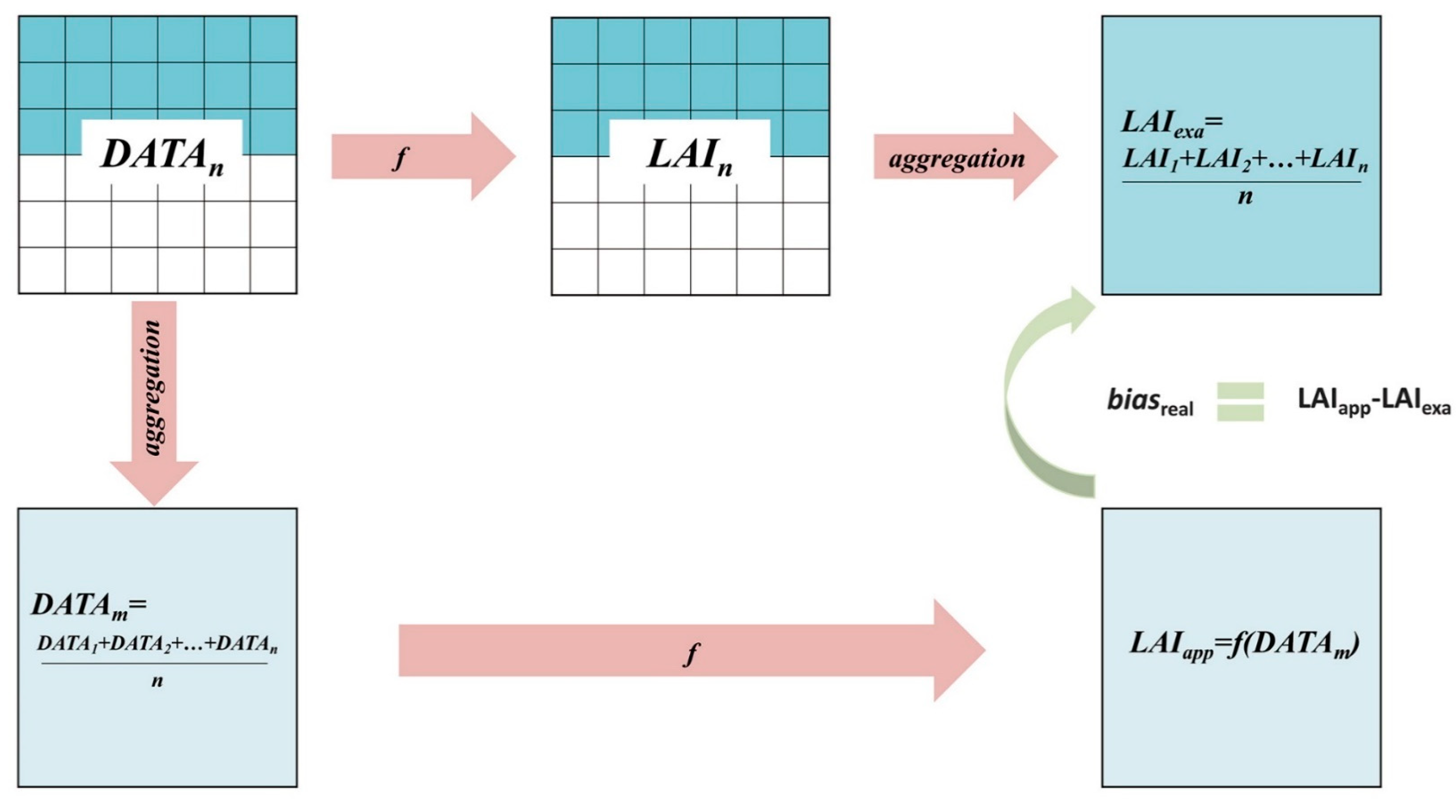
The LAI retrieval model f is constructed at fine spatial resolution. Applying f to fine-resolution data, then aggregating the resulting data to coarse resolution, yields the exact LAI ( L A I e x a ). The L A I e x a is the reference LAI at coarse resolution because leaf area follows the law of conservation of matter [10]. The approximate LAI ( L A I a p p ) is obtained by applying model f to coarse-resolution data, which are aggregated from fine-resolution data. The difference between L A I a p p and L A I e x a is the spatial scaling bias [23], as shown in Figure 4.
In the field of remote sensing, according to Equations (2) and (4), the real scaling bias of the inverted parameter can be expressed as follows:
b i a s R e a l = L A I a p p L A I e x a = f E X E f X = Δ = ln x A x G
Next, two LAI retrieval models with negative logarithmic form are used to derive the scaling bias of LAI.
The Beer–Lambert law is a negative logarithmic function [37,38]:
L A I = cos θ Ω G θ ln p θ
where G θ represents the leaf projection coefficient on a plane perpendicular to the observation direction θ . θ is set to 30 degrees in Table 1. Assuming that foliage angles are distributed spherically, G θ is set to 0.5 [39]. Ω is the foliage clumping index, which is set as a constant according to the vegetation type [40,41]. Here, fine-resolution directional gap probability p θ is measured based on geometric features, and there is no scaling effect [42]. According to Equations (5) and (6), the scaling bias of LAI is:
b i a s A M G M = cos θ Ω G θ ln A p θ G p θ
where G p θ and A p θ are the geometric and arithmetic means of fine resolution p θ within a coarse-resolution pixel, respectively.
The NDVI-LAI semi-empirical transfer function also has a negative logarithmic form [43],
L A I = 1 K L A I ln N D V I N D V I max N D V I min N D V I max
where N D V I max is the asymptotic value of NDVI, which is obtained when LAI is greater than 8; N D V I min is the NDVI value for bare soil; K L A I represents the extinction coefficient, which relates to vegetation spatial structure and vegetation canopy structure [33,44]. Here, the directional gap probability is obtained using Equation (9) [41]:
p ρ N I R , ρ R = ρ N I R     ρ R ρ N I R   +   ρ R N D V I max N D V I min N D V I max
where ρ N I R and ρ R represent near-infrared and red reflectances, respectively. To avoid introducing the scaling bias of NDVI into the directional gap probability calculation at coarse resolution, we use the aggregated reflectance rather than the aggregated NDVI. According to Equations (5) and (8), the scaling bias of LAI is:
b i a s ρ _ A M G M = 1 K L A I ln p A ρ N I R , A ρ R G p ρ N I R , ρ R
where G p ρ N I R , ρ R is the geometric mean of fine resolution p ρ N I R , ρ R within a coarse-resolution pixel, and p A ρ N I R , A ρ R is the directional gap probability at coarse resolution estimated based on the arithmetic mean of the fine-resolution reflectance.

3.2. Calculate Factor μ

The second derivative term μ absorbs the impact of all higher-order moments associated with X in Equation (2). p θ is measured according to the canopy geometry [45], the value at coarse resolution is equal to the arithmetic mean of fine-resolution directional gap probability p θ . The value of μ can be derived directly from Equation (2). It can also be obtained using the second derivative. Therefore, the μ value based on Equation (6) is shown as follows:
μ A M G M = 2 b i a s A M G M V a r X = 1 Ω G θ cos θ × c k 2
where c k is related to p θ .
When the directional gap probability calculation involves a nonlinear model, such as Equation (8), the value of p A ρ N I R , A ρ R is not equal to the value of A p ρ N I R , ρ R (the arithmetic mean of fine-resolution p ρ N I R , ρ R ). The first-order derivative term cannot be eliminated. Thus, Equation (2) is modified as follows:
Δ = 1 2 μ ρ _ A M G M V a r ( X ) + f x M k = 1 N x k x M N
where x k is the kth value of p ρ N I R , ρ R within a coarse-resolution pixel; x M represents the directional gap probability at coarse resolution, i.e., p A ρ N I R , A ρ R ; μ ρ _ A M G M is the second derivative term and V a r X is the mean square error. According to Equations (10) and (12), the value of μ based on Equation (8) can be expressed as follows:
μ ρ _ A M G M = 2 b i a s ρ _ A M G M + f x M K = 1 N x k x M N   V a r ( X ) = 1 k L A I × c k 2
where c k is related to p ρ N I R , ρ R .

3.3. Simplify the AM–GM Algorithm

The application of the AM–GM algorithm is limited by its use of fine-resolution remote sensing data. In this section, this algorithm was simplified. According to Equation (A4) in Appendix A and Equation (10), the following formula can be derived:
b i a s ρ _ A M G M = L A I a p p × 1 ln G p ρ N I R , ρ R ln p A ρ N I R , A ρ R
where ln p A ρ N I R , A ρ R represents the logarithm of the directional gap probabilities at coarse resolution and ln G p ρ N I R , ρ R represents the logarithm of the geometric mean of fine resolution p ρ N I R , ρ R within a coarse-resolution pixel.
A linear relationship between ln p A ρ N I R , A ρ R and ln G p ρ N I R , ρ R was found between two specific resolutions; the relationship will be described in further detail in the Results section. Equation (14) can be simplified according to the linear relationship, as follows:
b i a s ρ _ A M G M = L A I a p p × b ln p A ρ N I R , A ρ R a
where parameters a and b are constants between two specific resolutions. According to Equation (15), the scaling bias of LAI can be calculated based on the coarse resolution data.

4. Results

4.1. Validation Results of the AM–GM Algorithm

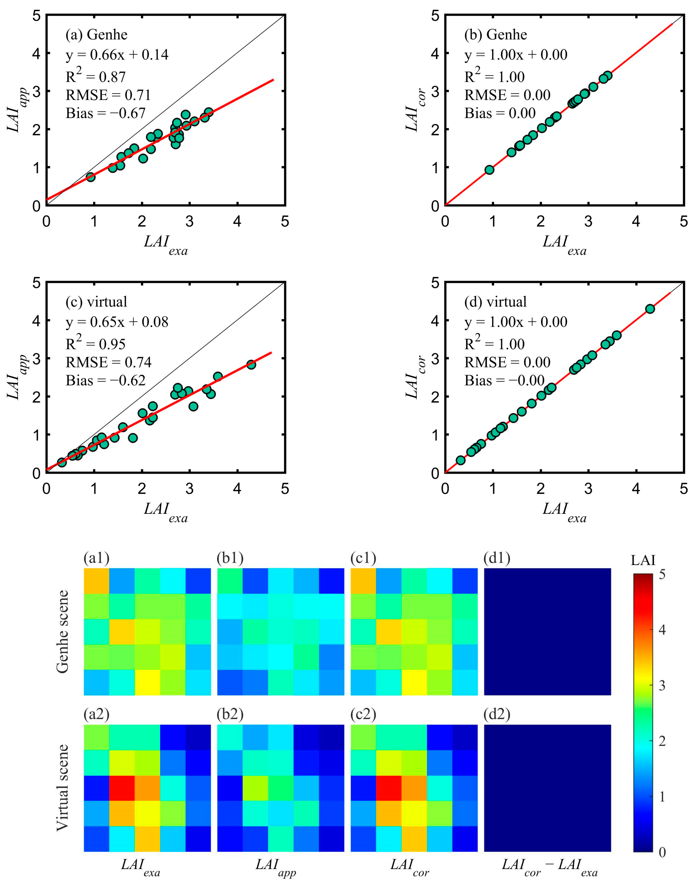
Firstly, this study validates the correction effectiveness of the AM–GM algorithm when the Beer–Lambert law is the LAI retrieval model. The computation of LAI scaling bias based on the Beer–Lambert law is derived in Equation (7). Figure 5 and Table 3 show the magnitude of the scaling bias before and after correction. Before the correction, the retrieval L A I a p p at coarse resolution exhibits significant negative scaling biases (bias = −0.67 and bias = −0.62). After correction, the bias and RMSE values between L A I c o r and L A I e x a are both reduced to almost 0. Furthermore, the spatial distribution of the corrected values L A I c o r coincides with L A I e x a . These results indicate that the AM–GM algorithm is effective when the Beer–Lambert law is the retrieval model.
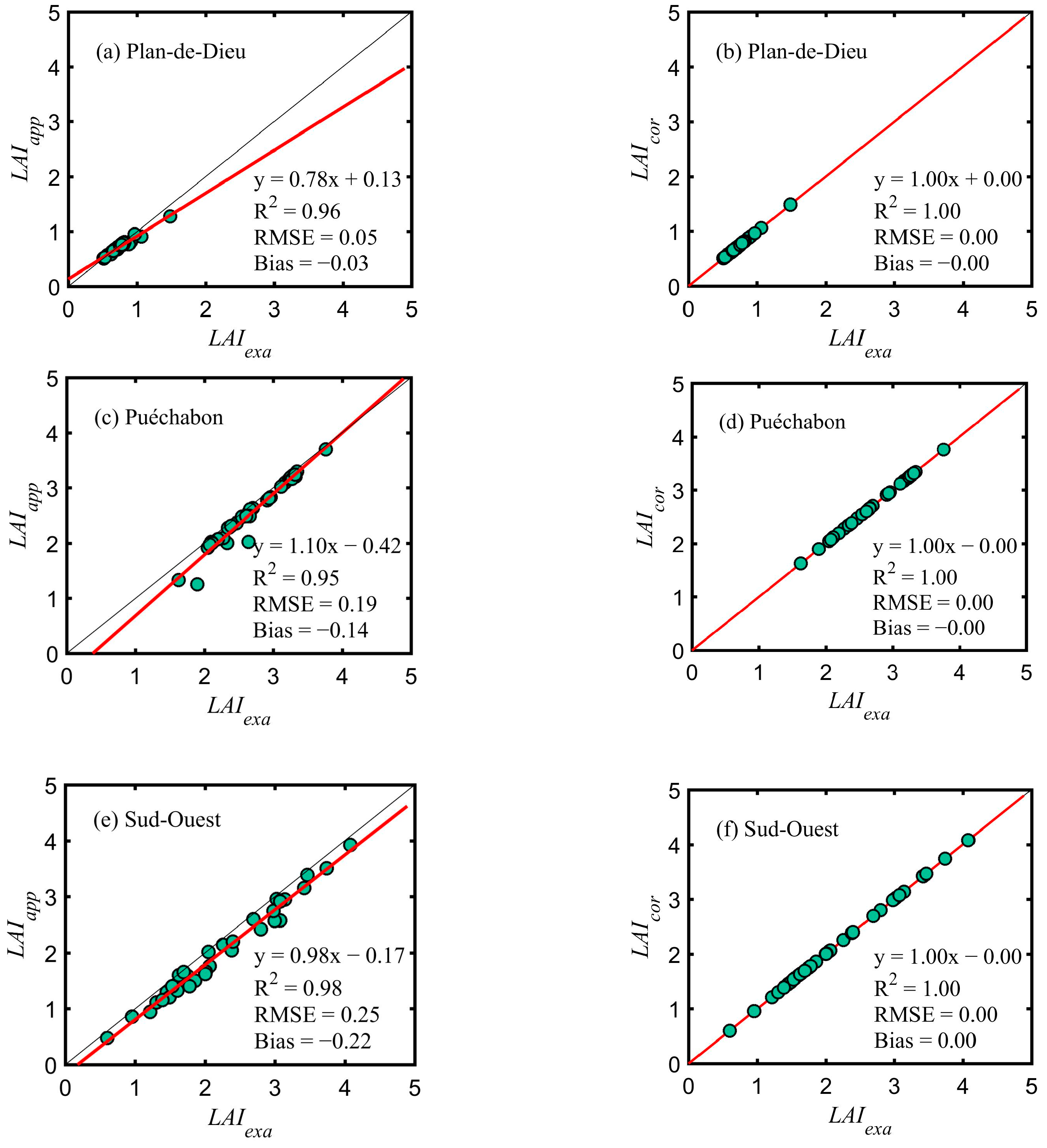
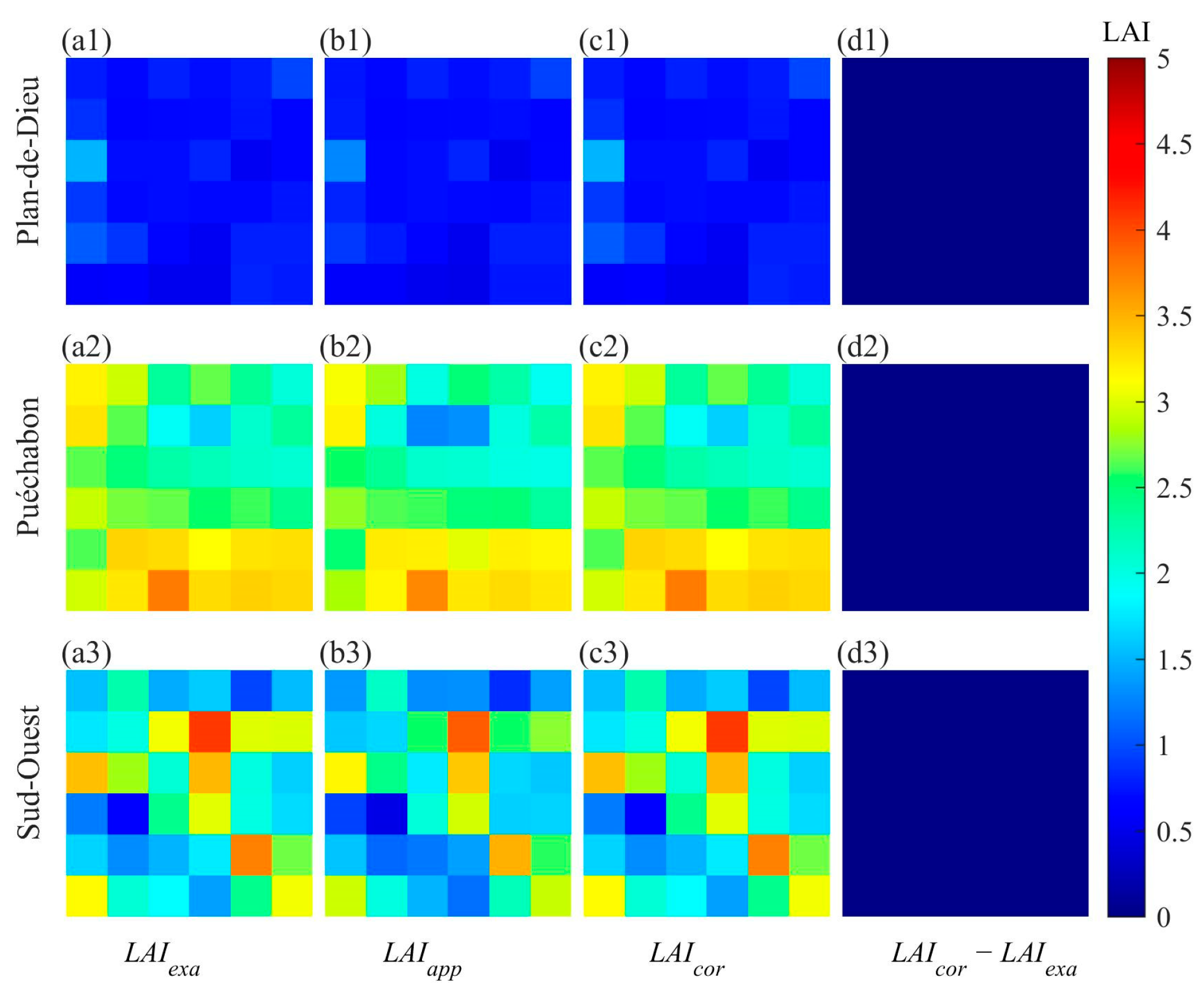
We also assess the correction effectiveness when the NDVI-LAI semi-empirical transfer function is the LAI retrieval model. The equation for the calculation of LAI scaling bias is shown in Equation (10). Figure 6 and Table 3 show that the scaling biases are small at the Plan-de-Dieu site, with RMSE = 0.05 and bias = −0.03; moderate at the Puéchabon site, with RMSE= 0.19 and bias = −0.14; and high at the Sud-Ouest site, with RMSE = 0.25 and bias = −0.22. After correction, the values of RMSE and bias between L A I c o r and L A I e x a are also deduced to almost 0, and all spots are clustered on the 1:1 line. Meanwhile, the spatial distributions of L A I c o r coincide with L A I e x a . These results indicate that the AM–GM algorithm is effective when the NDVI-LAI semi-empirical transfer function is the retrieval model.

4.2. Analysis of LAI Scaling Bias

Two figures are used to analyze the LAI scaling bias based on three aspects: spatial resolution, model nonlinearity, and surface heterogeneity. In Figure 7, we calculate the average of LAI scaling bias for each scene and site using the AM–GM algorithm at multiple scales. In Figure 8, the values of μ and V a r X are calculated for each coarse pixel based on Equations (11) and (13).
  • Spatial resolution.
When the spatial resolution for LAI estimation becomes coarser, the scaling bias of LAI increases. The scaling bias of LAI between two close resolutions may also be large. In Figure 7, as the spatial resolution moves from 1 to 45, the value of LAI scaling bias decreases and the LAI scaling bias increases. For the Beer–Lambert law, the scaling bias of L A I a p p at 5 m spatial resolution relative to L A I e x a estimated at 1 m spatial resolution is large, as shown in Figure 7a.
  • Model nonlinearity.
When the LAI value increases, the degree of model nonlinearity also rises. This is because the model nonlinearity is related to 1 / c k 2 in Equations (11) and (13), and the value of c k is related to directional gap probability. When the value of c k for a coarse pixel is small, the directional gap probability of this pixel is also small, and the LAI value is large [46]. For example, in Figure 6, the exact LAI values for row 2 to 4 in the fourth column of the Sud-Ouest site are relatively large. Correspondingly, in Figure 8, the values of μ ρ _ A M G M calculated by the AM–GM algorithm for these pixels are also relatively high.
  • Surface heterogeneity.
When vegetation in a coarse pixel has different growing seasons, the degree of surface heterogeneity is high. The Sud-Ouest site includes nine crops with various growing seasons, while both the Plan-de-Dieu and Puéchabon sites have a relatively singular growing season. Therefore, Figure 8 shows that the V a r X values of the Sud-Ouest site are larger than those of the other two sites.

4.3. Scaling Bias Calculated by the Simplified Algorithm

Although the AM–GM algorithm can correct the LAI scaling bias more accurately, it requires fine-resolution remote sensing data, which limits the applicability of this algorithm. The simplified AM–GM algorithm does not use fine-resolution data.
Figure 9 shows that linear relationships between the two quantities ln p A ρ N I R , A ρ R and ln G p ρ N I R , ρ R are observed at four croplands between the fine and multiple resolutions (200 m, 500 m, 1000 m, and 1500 m), respectively. Due to the limited sample size, this relationship is not built at the spatial resolution of 3 km. The parameters a and b for simplified AM–GM algorithm in Equation (15) are shown in Table 4.
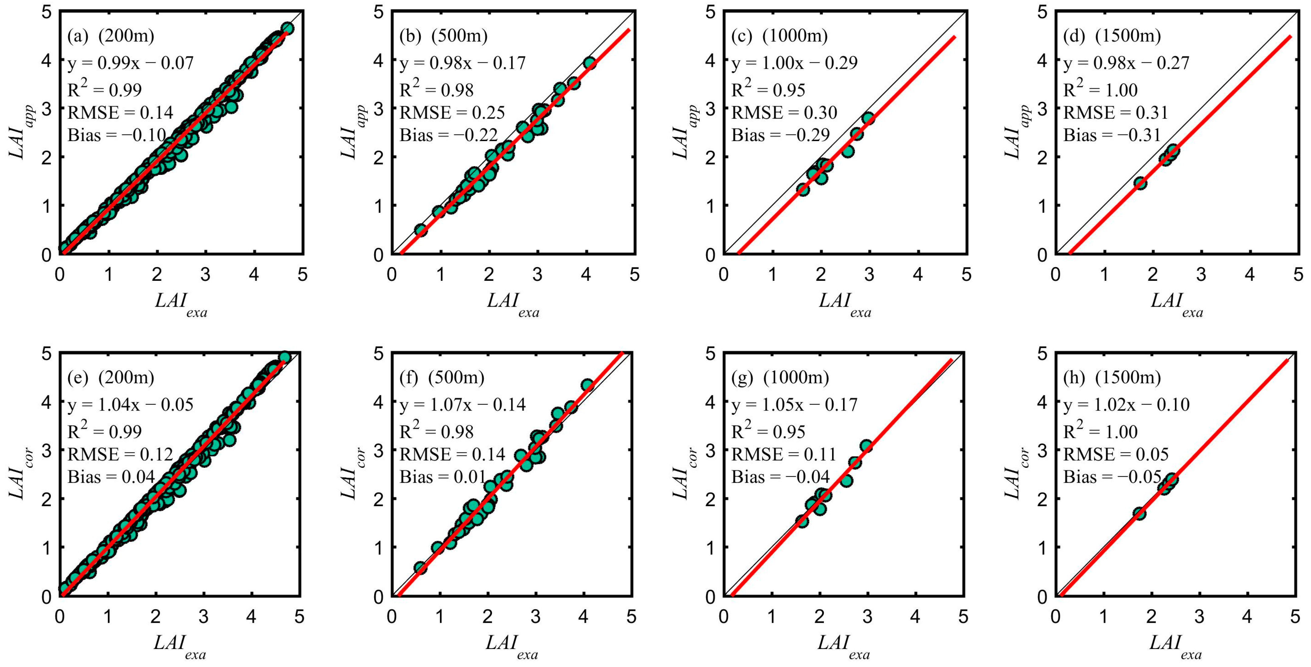
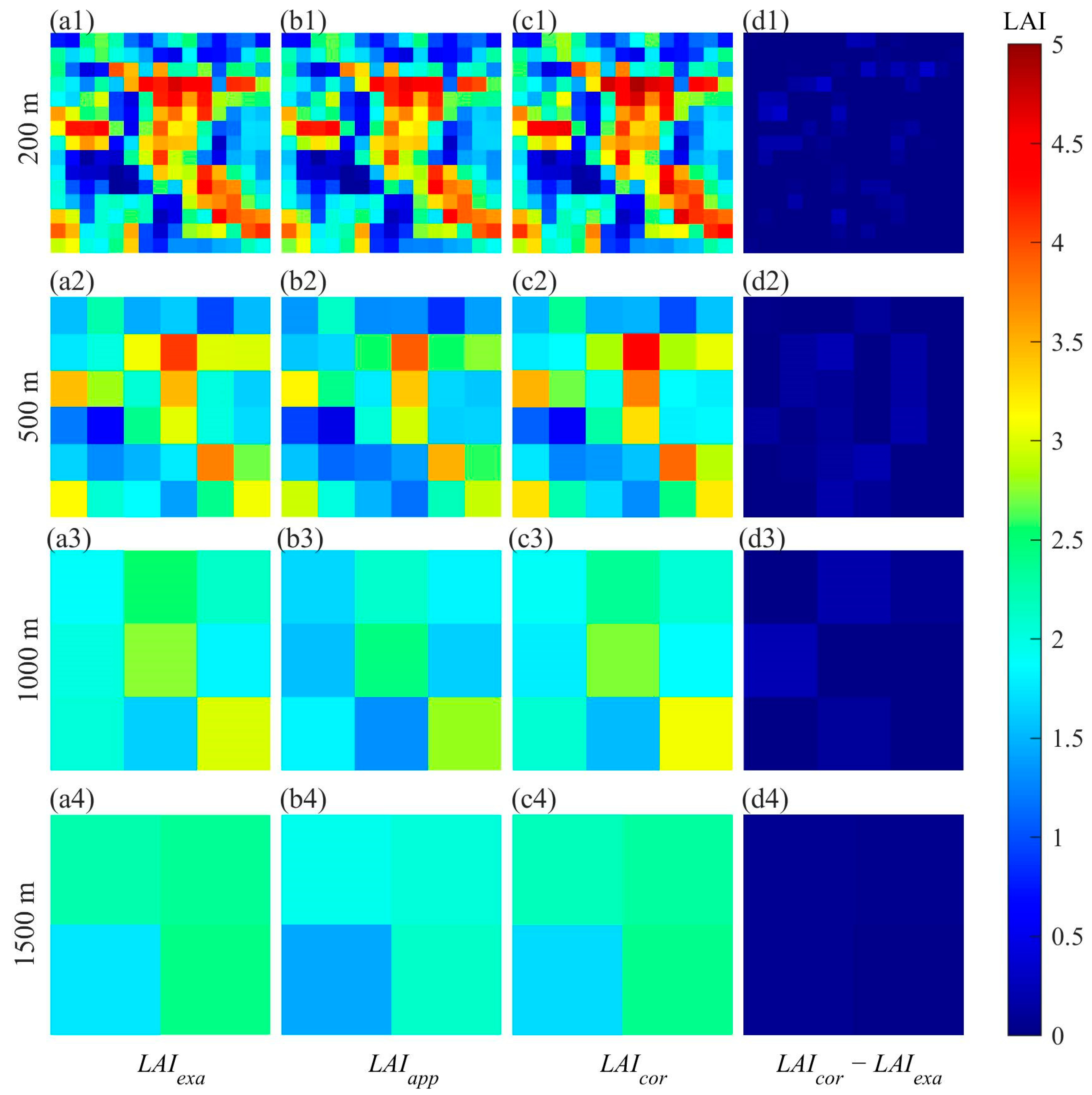
The simplified AM–GM algorithm corrected the scaling bias of LAI at multiple scales over the Sud-Ouest site. Figure 10 shows that after correction, the values of L A I c o r are close to the values of L A I e x a . The absolute values of bias at the Sud-Ouest site decrease from 0.10, 0.22, 0.29, and 0.31 to 0.04, 0.01, 0.04, and 0.05 at 200 m, 500 m, 1000 m, and 1500 m, respectively. Moreover, Figure 11 shows that the spatial distributions of L A I c o r are well corrected, particularly at spatial resolutions of 1000 m and 1500 m. Therefore, the simplified AM–GM algorithm, which does not use fine-resolution images, is feasible.

5. Discussion

5.1. Algorithm Comparison

Prior work has documented the flaws in the TSEM algorithm resulting from the second-order stationary hypothesis, which assumes that the mean of a random function is a constant [30]. The AM–GM algorithm considered the higher-order moments, i.e., the skewness that measures the asymmetry, and the kurtosis that measures the heaviness of the tails of distribution without discarding [31]. We compared the values of μ calculated using the AM–GM and TSEM algorithms in Table 5. The results show bias in μ up to 7.16. However, the numerical discrepancies of the input variable used for μ calculation are less than 0.02. It is inferred that the μ value is sensitive to the input variable. On the heterogeneous surfaces, the skewness and kurtosis of the random variable may be large, and the AM–GM algorithm may exhibit a better performance for the computation of μ and LAI scaling bias.
In the improved CGM, the relative errors decreased from 3.35%, 11.01%, and 19.62% to an average of 0.28%, 1.48%, and 5.16%, respectively, at kilometer scales [26]. Jiang et al. indicated that the LAI scaling bias decreased to around 0.27 by the TSEM, Wavelet-Fractal (WF), and Fractal theory (TT) [30]. We determine that the AM–GM algorithm decreases the LAI scaling bias to almost zero. The simplified AM–GM algorithm decreases relative error from 16.07% to 4.3% at 1 km resolution. The LAI scaling bias decreases from 0.10, 0.22, 0.29, and 0.31 to 0.04, 0.01, 0.04, and 0.05 at 200 m, 500 m, 1000 m, and 1500 m resolutions, respectively. On the heterogeneous surfaces, the correction effect is comparable or even better. The simplified algorithm, TSEM, WF, or TT, does not perform well at homogeneous sites.

5.2. The Influence of NDVI Aggregation on the AM–GM Algorithm

To minimize errors of LAI estimation, care should be taken in relation to the scale issue of NDVI. In the past, studies usually used the vegetation index (VI) to calculate the scaling bias of LAI [30]. However, most of the equations for VIs are nonlinear, including the NDVI equation related to reflectance. The scaling bias of NDVI complicates the evaluation of the LAI scaling bias on the heterogeneous surface. Table 6 shows that the aggregated NDVI results in inaccurate estimates of LAI scaling bias based on the AM–GM algorithm. Additionally, the bias may be a positive or a negative value. In particular, several approaches have been provided to reconstruct time-series data for NDVI using both fine- and coarse-resolution NDVI data. The discussion in 5.2 may indicate that if the time-series data are used for LAI estimation, the scaling bias of NDVI should be considered during data reconstruction.

5.3. Limitation of the AM–GM Algorithm

This algorithm is only suitable for negative logarithmic functions because Holder’s defect provides an accurate expression of the AM–GM inequality for negative logarithmic functions [31]. This limitation restricts the application of the AM–GM algorithm. In addition, this study corrected LAI scaling bias due to the spatial heterogeneity of vegetation growth but did not consider the model difference caused by vegetation types. In the future, we plan to further improve this algorithm for use with mixed land surfaces.

6. Conclusions

We found that scaling bias in remote sensing can be accurately expressed by the AM–GM inequality for negative logarithmic function. Based on this relationship, the AM–GM algorithm was proposed. This algorithm avoids the influence of the second-order stationary hypothesis. In addition, the aggregation of NDVI, which was ignored in previous research about scaling bias correction, is considered in the AM–GM algorithm. In this study, we validated the AM–GM algorithm at two simulated scenes and three sites, proving its effectiveness in the correction and analysis of the LAI scaling bias at coarse resolution.
In addition, upon analyzing the second derivative term, we identified a positive correlation between the LAI value and the degree of model nonlinearity. This means that as the LAI value increases, the nonlinearity in the model also increases. It was also observed that when the spatial resolution is coarse and the surface heterogeneity increases, there is a greater scaling bias in the LAI estimation. Adjusting for the LAI scaling bias was critical in the above three cases.
Furthermore, we identified a linear statistical relationship between two quantities related to directional gap probability between two specific scales. The AM–GM algorithm is simplified by the relationship. The results indicate that the simplified algorithm can practically correct the scaling bias without the requirement of fine-resolution remote sensing data. In conclusion, the correction effect of this algorithm is reliable. Future work includes the improvement of this algorithm on mixed land surfaces.

Author Contributions

Conceptualization, R.S.; Methodology, J.Z.; Validation, J.Z.; Formal analysis, J.Z.; Resources, D.X.; Writing—original draft, J.Z.; Writing—review & editing, R.S., Z.X. and L.Z.; Supervision, J.Z.; Funding acquisition, R.S. All authors have read and agreed to the published version of the manuscript.

Funding

This research was funded by the National Natural Science Foundation of China (42271330) and the National Key R&D Program of China (2021YFB3901201).

Data Availability Statement

The data presented in this study are available upon request from the corresponding author.

Acknowledgments

Thanks to Jialun Zhou (School of Electrical and Information Engineering, Zhengzhou university, China) for his contribution to the derivation of mathematical formulas.

Conflicts of Interest

The authors declare no conflict of interest.

Appendix A

Based on the Beer–Lambert law, the L A I e x a is estimated as follows:
L A I e x a = k = 1 N cos θ Ω G θ ln ( p k ( θ ) ) N = cos θ Ω G θ ln G p k θ
where N is the quantity of subpixels within a coarse resolution pixel; k is equal to 1 to N; foliage projection function G θ is set to 0.5; and cos θ is set to 1. G p k θ is the geometric mean of fine spatial resolution p k θ within a coarse resolution pixel. L A I a p p is:
L A I a p p = cos θ Ω G θ ln k = 1 N p k θ N = cos θ Ω G θ ln A p k θ
where A p k θ is the arithmetic mean of p k θ within a coarse resolution pixel. Based on the semiempirical transfer function, L A I e x a is:
L A I e x a = 1 K L A I ln G p ρ N I R k , ρ R k
where K L A I is the extinction coefficient, p ρ N I R k , ρ R k represents the kth directional gap probability at fine spatial resolution, which is estimated by Equation (9) in the body of the article. G p ρ N I R k , ρ R k is the geometric mean of p ρ N I R k , ρ R k within a coarse spatial resolution. The approximate LAI is:
L A I a p p = 1 K L A I ln p A ρ N I R k , A ρ R k
where A ρ N I R k and A ρ R k are the arithmetic means of red reflectance ρ R k and near-infrared reflectance ρ N I R k within a coarse resolution pixel, respectively. p A ρ N I R , A ρ R is the directional gap probability of that coarse-resolution pixel.

Appendix B

When the scaling bias of LAI is calculated using the TSEM algorithm, an approximate value directly obtains as follows:
b i a s T S E M 1 2 f x A k = 1 N x k x A N 2 = 1 2 μ T S E M V a r X T S E M
where N is the quantity of subpixels within a coarse resolution pixel, x A is the arithmetic mean of the input variable X = x 1 , x 2 , , x N , and f x A is the second derivative at x A , which is denoted by μ T S E M . x k is the kth input variable in a coarse pixel. V a r X T S E M is the variance of X .

References

  1. Baret, F.; Weiss, M.; Lacaze, R.; Camacho, F.; Makhmara, H.; Pacholcyzk, P.; Smets, B. GEOV1: LAI and FAPAR essential climate variables and FCOVER global time series capitalizing over existing products. Part1: Principles of development and production. Remote Sens. Environ. 2013, 137, 299–309. [Google Scholar] [CrossRef]
  2. Wang, J.; Sun, R.; Zhang, H.; Xiao, Z.; Zhu, A.; Wang, M.; Yu, T.; Xiang, K. New Global MuSyQ GPP/NPP Remote Sensing Products From 1981 to 2018. IEEE J. Sel. Top. Appl. Earth Observ. Remote Sens. 2021, 14, 5596–5612. [Google Scholar] [CrossRef]
  3. Chen, Z.; Jia, K.; Wei, X.; Liu, Y.; Zhan, Y.; Xia, M.; Yao, Y.; Zhang, X. Improving leaf area index estimation accuracy of wheat by involving leaf chlorophyll content information. Comput. Electron. Agric. 2022, 196, 106902. [Google Scholar] [CrossRef]
  4. Cortés, J.; Mahecha, M.D.; Reichstein, M.; Myneni, R.B.; Chen, C.; Brenning, A. Where Are Global Vegetation Greening and Browning Trends Significant? Geophys. Res. Lett. 2021, 48, e2020GL091496. [Google Scholar] [CrossRef]
  5. Chen, C.; Park, T.; Wang, X.H.; Piao, S.L.; Xu, B.D.; Chaturvedi, R.K.; Fuchs, R.; Brovkin, V.; Ciais, P.; Fensholt, R.; et al. China and India lead in greening of the world through land-use management. Nat. Sustain. 2019, 2, 122–129. [Google Scholar] [CrossRef]
  6. Yu, T.; Zhang, Q.; Sun, R. Comparison of Machine Learning Methods to Up-Scale Gross Primary Production. Remote Sens. 2021, 13, 2448. [Google Scholar] [CrossRef]
  7. Chen, J.M.; Ju, W.M.; Ciais, P.; Viovy, N.; Liu, R.G.; Liu, Y.; Lu, X.H. Vegetation structural change since 1981 significantly enhanced the terrestrial carbon sink. Nat. Commun. 2019, 10, 4259. [Google Scholar] [CrossRef] [Green Version]
  8. Garrigues, S.; Allard, D.; Baret, F.; Weiss, M. Influence of the spatial heterogeneity on the non-linear estimation of Leaf Area Index from moderate resolution remote sensing data. Remote Sens. Environ. 2006, 105, 286–298. [Google Scholar] [CrossRef]
  9. Liu, W.H.; Shi, J.C.; Liang, S.L.; Zhou, S.G.; Cheng, J. Simultaneous retrieval of land surface temperature and emissivity from the FengYun-4A advanced geosynchronous radiation imager. Int. J. Digit. Earth 2022, 15, 198–225. [Google Scholar] [CrossRef]
  10. Wu, H.; Li, Z.-L. Scale Issues in Remote Sensing: A Review on Analysis, Processing and Modeling. Sensors 2009, 9, 1768–1793. [Google Scholar] [CrossRef]
  11. Zhang, J.; Wang, J.; Sun, R.; Zhou, H.; Zhang, H. A Model-Downscaling Method for Fine-Resolution LAI Estimation. Remote Sens. 2020, 12, 4147. [Google Scholar] [CrossRef]
  12. Deng, F.; Chen, J.M.; Plummer, S.; Chen, M.; Pisek, J. Algorithm for global leaf area index retrieval using satellite imagery. IEEE Trans. Geosci. Remote Sens. 2006, 44, 2219–2229. [Google Scholar] [CrossRef] [Green Version]
  13. Liang, S. Numerical experiments on the spatial scaling of land surface albedo and leaf area index. Remote Sens. Rev. 2000, 19, 225–242. [Google Scholar] [CrossRef]
  14. Tao, X.; Yan, B.; Wang, K.; Wu, D.; Fan, W.; Xu, X.; Liang, S. Scale transformation of Leaf Area Index product retrieved from multiresolution remotely sensed data: Analysis and case studies. Int. J. Remote Sens. 2009, 30, 5383–5395. [Google Scholar] [CrossRef]
  15. Yin, G.F.; Li, J.; Liu, Q.H.; Li, L.H.; Zeng, Y.L.; Xu, B.D.; Yang, L.; Zhao, J. Improving Leaf Area Index Retrieval Over Heterogeneous Surface by Integrating Textural and Contextual Information: A Case Study in the Heihe River Basin. IEEE Geosci. Remote Sens. Lett. 2015, 12, 359–363. [Google Scholar] [CrossRef]
  16. Xu, B.D.; Li, J.; Park, T.J.; Liu, Q.H.; Zeng, Y.L.; Yin, G.F.; Yan, K.; Chen, C.; Zhao, J.; Fan, W.L.; et al. Improving leaf area index retrieval over heterogeneous surface mixed with water. Remote Sens. Environ. 2020, 240, 111700. [Google Scholar] [CrossRef]
  17. Fang, H.; Baret, F.; Plummer, S.; Schaepman-Strub, G. An Overview of Global Leaf Area Index (LAI): Methods, Products, Validation, and Applications. Rev. Geophys. 2019, 57, 739–799. [Google Scholar] [CrossRef]
  18. Fisher, R.A.; Koven, C.D. Perspectives on the Future of Land Surface Models and the Challenges of Representing Complex Terrestrial Systems. J. Adv. Model. Earth Syst. 2020, 12, e2018MS001453. [Google Scholar] [CrossRef] [Green Version]
  19. Zhao, W.; Fan, W. Quantitative Representation of Spatial Heterogeneity in the LAI Scaling Transfer Process. IEEE Access 2021, 9, 83851–83862. [Google Scholar] [CrossRef]
  20. Jin, Z.; Tian, Q.; Chen, J.M.; Chen, M. Spatial scaling between leaf area index maps of different resolutions. J. Environ. Manag. 2007, 85, 628–637. [Google Scholar] [CrossRef]
  21. Raffy, M. Change of scale in models of remote sensing: A general method for spatialization of models. Remote Sens. Environ. 1992, 40, 101–112. [Google Scholar] [CrossRef]
  22. Hu, Z.; Islam, S. A framework for analyzing and designing scale invariant remote sensing algorithms. IEEE Trans. Geosci. Remote. Sens. 1997, 35, 747–755. [Google Scholar] [CrossRef] [Green Version]
  23. Jiang, J.; Liu, X.; Liu, C.; Wu, L.; Xia, X.; Liu, M.; Du, Z. Analyzing the Spatial Scaling Bias of Rice Leaf Area Index From Hyperspectral Data Using Wavelet-Fractal Technique. IEEE J. Sel. Top. Appl. Earth Observ. Remote Sens. 2015, 8, 3068–3080. [Google Scholar] [CrossRef]
  24. Wu, L.; Liu, X.; Qin, Q.; Zhao, B.; Ma, Y.; Liu, M.; Jiang, T. Scaling Correction of Remotely Sensed Leaf Area Index for Farmland Landscape Pattern With Multitype Spatial Heterogeneities Using Fractal Dimension and Contextural Parameters. IEEE J. Sel. Top. Appl. Earth Observ. Remote Sens. 2018, 11, 1472–1481. [Google Scholar] [CrossRef]
  25. Wu, L.; Qin, Q.; Liu, X.; Ren, H.; Wang, J.; Zheng, X.; Ye, X.; Sun, Y. Spatial Up-Scaling Correction for Leaf Area Index Based on the Fractal Theory. Remote Sens. 2016, 8, 197. [Google Scholar] [CrossRef] [Green Version]
  26. Chen, H.; Wu, H.; Li, Z.-L.; Tu, J. An Improved Computational Geometry Method for Obtaining Accurate Remotely Sensed Products via Convex Hulls With Dynamic Weights: A Case Study With Leaf Area Index. IEEE J. Sel. Top. Appl. Earth Observ. Remote Sens. 2019, 12, 2308–2319. [Google Scholar] [CrossRef]
  27. Wang, J.P.; Wu, X.D.; Wen, J.G.; Xiao, Q.; Gong, B.C.; Ma, D.J.; Cui, Y.R.; Lin, X.W.; Bao, Y.F. Upscaling in Situ Site-Based Albedo Using Machine Learning Models: Main Controlling Factors on Results. IEEE Trans. Geosci. Remote Sens. 2022, 60, 3095153. [Google Scholar] [CrossRef]
  28. Wu, X.D.; Wen, J.G.; Tang, R.Q.; Wang, J.P.; Zeng, Q.C.; Li, Z.; You, D.Q.; Lin, X.W.; Gong, B.C.; Xiao, Q. Quantification of the uncertainty in multiscale validation of coarse-resolution satellite albedo products: A study based on airborne CASI data. Remote Sens. Environ. 2023, 287, 113465. [Google Scholar] [CrossRef]
  29. Chen, Y.G. Fractal Modeling and Fractal Dimension Description of Urban Morphology. Entropy 2020, 22, 961. [Google Scholar] [CrossRef]
  30. Jiang, J.; Ji, X.; Yao, X.; Tian, Y.; Zhu, Y.; Cao, W.; Cheng, T. Evaluation of Three Techniques for Correcting the Spatial Scaling Bias of Leaf Area Index. Remote Sens. 2018, 10, 221. [Google Scholar] [CrossRef] [Green Version]
  31. Becker, R. The Variance Drain and Jensen’s Inequality. CAEPR Work. Pap. 2012, 2004–2012. [Google Scholar] [CrossRef] [Green Version]
  32. Li, W.; Mu, X. Using fractal dimension to correct clumping effect in leaf area index measurement by digital cover photography. Agric. For. Meteorol. 2021, 311, 108695. [Google Scholar] [CrossRef]
  33. Shi, Y.; Wang, J.; Wang, J.; Qu, Y. A Prior Knowledge-Based Method to Derivate High-Resolution Leaf Area Index Maps with Limited Field Measurements. Remote Sens. 2017, 9, 13. [Google Scholar] [CrossRef] [Green Version]
  34. Zhang, X.; Yan, G.; Li, Q.; Li, Z.-L.; Wan, H.; Guo, L. Evaluating the fraction of vegetation cover based on NDVI spatial scale correction model. Int. J. Remote Sens. 2006, 27, 5359–5372. [Google Scholar] [CrossRef]
  35. Qi, J.; Xie, D.; Yin, T.; Yan, G.; Gastellu-Etchegorry, J.; Li, L.; Zhang, W.; Mu, X.; Norford, L. LESS: LargE-Scale remote sensing data and image simulation framework over heterogeneous 3D scenes. Remote Sens. Environ. 2019, 221, 695–706. [Google Scholar] [CrossRef]
  36. Xu, Y.; Xie, D.; Qi, J.; Yan, G.; Mu, X.; Zhang, W. Influence of woody elements on nadir reflectance of forest canopy based on simulations by using the LESS model. J. Remote Sens. 2021, 25, 1138–1151. [Google Scholar]
  37. Nilson, T. A theoretical analysis of frequency of gaps in plant stands. Agric. Meteorol. 1971, 8, 25. [Google Scholar] [CrossRef]
  38. Wang, W.-M.; Li, Z.-L.; Su, H.-B. Comparison of leaf angle distribution functions: Effects on extinction coefficient and fraction of sunlit foliage. Agric. For. Meteorol. 2007, 143, 106–122. [Google Scholar] [CrossRef]
  39. Yan, G.; Hu, R.; Luo, J.; Weiss, M.; Jiang, H.; Mu, X.; Xie, D.; Zhang, W. Review of indirect optical measurements of leaf area index: Recent advances, challenges, and perspectives. Agric. For. Meteorol. 2019, 265, 390–411. [Google Scholar] [CrossRef]
  40. Xiao, Z.; Liang, S.; Wang, J.; Chen, P.; Yin, X.; Zhang, L.; Song, J. Use of General Regression Neural Networks for Generating the GLASS Leaf Area Index Product From Time-Series MODIS Surface Reflectance. IEEE Trans. Geosci. Remote Sens. 2014, 52, 209–223. [Google Scholar] [CrossRef]
  41. Fang, H. Canopy clumping index (CI): A review of methods, characteristics, and applications. Agric. For. Meteorol. 2021, 303, 18. [Google Scholar] [CrossRef]
  42. Ryu, Y.; Nilson, T.; Kobayashi, H.; Sonnentag, O.; Law, B.E.; Baldocchi, D.D. On the correct estimation of effective leaf area index: Does it reveal information on clumping effects? Agric. For. Meteorol. 2010, 150, 463–472. [Google Scholar] [CrossRef]
  43. Tang, S.; Chen, J.; Zhu, Q.; Li, X.; Chen, M.; Sun, R.; Zhou, Y.; Deng, F.; Xie, D. LAI inversion algorithm based on directional reflectance kernels. J. Environ. Manag. 2007, 85, 638–648. [Google Scholar] [CrossRef]
  44. Baret, F.; Guyot, G. Potentials and limits of vegetation indices for LAI and APAR assessment. Remote Sens. Environ. 1991, 35, 161–173. [Google Scholar] [CrossRef]
  45. Chen, J.M.; Menges, C.H.; Leblanc, S.G. Global mapping of foliage clumping index using multi-angular satellite data. Remote Sens. Environ. 2005, 97, 447–457. [Google Scholar] [CrossRef]
  46. Ma, L.; Li, C.; Tang, B.; Tang, L.; Bi, Y.; Zhou, B.; Li, Z.-L. Impact of spatial LAI heterogeneity on estimate of directional gap fraction from SPOT-satellite data. Sensors 2008, 8, 3767–3779. [Google Scholar] [CrossRef] [Green Version]
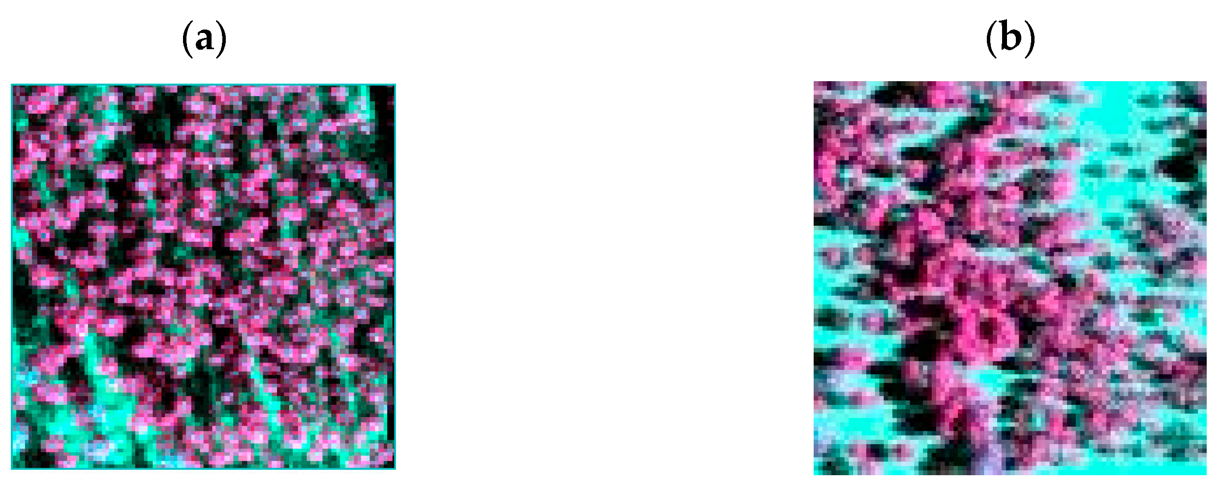
Figure 1. Standard false-color images of two forest scenes simulated using the LESS model: (a) Genhe scene; (b) virtual scene.
Remotesensing 15 03068 g001
Figure 2. Standard false-color images of the VALERI sites: (a) Plan-de-Dieu; (b) Puéchabon; (c) Sud-Ouest; (d) Les Alpilles; (e) Barrax; (f) Demmin; (g) Haouz.
Remotesensing 15 03068 g002
Figure 3. The flowchart for calculating, analyzing, and correcting the scaling bias of LAI using the AM–GM algorithm.
Remotesensing 15 03068 g003
Figure 4. Schematic diagram of the scaling bias of LAI at coarse resolution in quantitative remote sensing. The LAI retrieval model f is built at fine resolution. D A T A n represents the fine-resolution remote sensing data, and their corresponding LAI values at fine resolution ( L A I n ) are retrieved using f . L A I e x a represents the exact LAI at coarse resolution; this is acquired by averaging L A I n . D A T A m represents the coarse-resolution remote sensing data, which is obtained by averaging D A T A n . L A I a p p represents the approximate LAI at coarse resolution, which is obtained by applying model f to data D A T A m . b i a s r e a l represents the LAI scaling bias of a coarse resolution pixel, indicated by the difference between L A I a p p and L A I e x a .
Remotesensing 15 03068 g004
Figure 5. Numerical and spatial correction effectiveness of the AM–GM algorithm over two simulated scenes. The exact LAI ( L A I e x a , m2/m2) at 9 m spatial resolution is obtained from directional gap probability at 1 m spatial resolution and then aggregated to 9 m spatial resolution; the approximated LAI at 9 m spatial resolution ( L A I a p p , m2/m2) is evaluated from the aggregated directional gap probability at 9 m spatial resolution. The corrected L A I a p p ( L A I c o r , m2/m2) are achieved using the AM–GM algorithm at 9 m spatial resolution. The errors between L A I a p p and L A I e x a over (a) the Genhe scene and (c) the virtual scene; the errors between L A I c o r and L A I e x a over (b) the Genhe scene and (d) the virtual scene. (a1d1) spatial distributions of L A I e x a , L A I a p p , L A I c o r , and the difference between L A I e x a and L A I c o r over the Genhe scene; (a2d2) spatial distributions of L A I e x a , L A I a p p , L A I c o r , and the difference between L A I e x a and L A I c o r over the virtual scene.
Remotesensing 15 03068 g005
Figure 6. Numerical and spatial correction effectiveness of the AM–GM algorithm over three VALERI sites. The exact LAI ( L A I e x a , m2/m2) at 500 m spatial resolution is obtained from reflectance at 20 m spatial resolution and then aggregated to 500 m spatial resolution. The approximate LAI ( L A I a p p , m2/m2) at 500 m spatial resolution is estimated from the aggregated reflectance at 500 m spatial resolution. The corrected L A I a p p ( L A I c o r , m2/m2) is achieved using the AM–GM algorithm at 500 m spatial resolution. The errors between L A I a p p and L A I e x a over (a) the Plan-de-Dieu site, (c) the Puéchabon site, and (e) the Sud-Ouest site; the errors between L A I c o r and L A I e x a over (b) the Plan-de-Dieu site, (d) the Puéchabon site, and (f) the Sud-Ouest site. (a1d1) spatial distributions of L A I e x a , L A I a p p , L A I c o r , and the difference between L A I e x a and L A I c o r over the Plan-de-Dieu site; (a2d2) spatial distributions of L A I e x a , L A I a p p , L A I c o r , and the difference between L A I e x a and L A I c o r over the Puéchabon site; (a3d3) spatial distributions of L A I e x a , L A I a p p , L A I c o r , and the difference between L A I e x a and L A I c o r over the Sud-Ouest site.
Remotesensing 15 03068 g006aRemotesensing 15 03068 g006b
Figure 7. Average of LAI scaling bias calculated using the AM–GM algorithm at multiple scales for each scene and site: (a) based on the Beer–Lambert Law at two LESS simulated scenes, and (b) based on the NDVI-LAI semi-empirical transfer function at three VALERI sites.
Remotesensing 15 03068 g007
Figure 8. Spatial distribution maps of the LAI scaling bias and two factors ( V a r X and μ ρ _ A M G M ) computed by the AM–GM algorithm based on the NDVI-LAI semi-empirical transfer function at 500 m resolution over three VALERI sites. (a1a3) the local variance of directional gap probability at the Plan-de-Dieu site, the Puéchabon site, and the Sud-Ouest site, respectively. (b1b3) the second derivative μ ρ _ A M G M absorbs the impact of all higher-order moments at the Plan-de-Dieu site, the Puéchabon site, and the Sud-Ouest site, respectively. (c1c3) the scaling bias of LAI at the Plan-de-Dieu site, the Puéchabon site, and the Sud-Ouest site, respectively.
Remotesensing 15 03068 g008
Figure 9. The statistical relationships between ln G p ρ N I R , ρ R and ln p A ρ N I R , A ρ R investigated at multiple resolutions, (a) 200 m, (b) 500 m, (c) 1000 m, and (d) 1500 m, over Les Alpilles, Barrax, Demmin, and Haouz cropland sites.
Remotesensing 15 03068 g009
Figure 10. Correction of LAI scaling bias using the simplified AM–GM algorithm at multiple resolutions (200 m, 500 m, 1000 m, and 1500 m) over the Sud-Ouest site. Panels (ad) show the errors between L A I a p p and L A I e x a before correction, while panels (eh) show the errors after correction.
Remotesensing 15 03068 g010
Figure 11. Spatial distributions of the exact LAI ( L A I e x a ), approximate LAI ( L A I a p p ), corrected LAI ( L A I c o r ), and the differences between L A I c o r and L A I e x a at multiple resolutions (200 m, 500 m, 1000 m, and 1500 m) over the Sud-Ouest site. (a1d1) represent L A I e x a , L A I a p p , L A I c o r , and the difference between L A I c o r and L A I e x a at 200 m spatial resolution, respectively; (a2d2) represent L A I e x a , L A I a p p , L A I c o r , and the difference between L A I c o r and L A I e x a at 500 m spatial resolution, respectively; (a3d3) represent L A I e x a , L A I a p p , L A I c o r , and the difference between L A I c o r and L A I e x a at 1000 m spatial resolution, respectively; (a4d4) represent L A I e x a , L A I a p p , L A I c o r , and difference between L A I c o r and L A I e x a at 1500 m spatial resolution, respectively.
Remotesensing 15 03068 g011
Table 1. Parameter settings of the LESS model.
SensorParameter ValueOptical DatabaseParameter Value
TypeOrthographicLarch BranchGround Measurements
Width (pixels)45Brown LoamGround Measurements
Height (pixels)45Larch LeafGround Measurements
Samples (/pixel)64TerrainParameter Value
Spectral Bands482:60, 561.5:57, 654.5:37, 865:28TypePlane
Image FormatSpectrumXSize (m)45
NoData Value−1YSize (m)45
Width Extent (m)45BRDF TypeLambertian
Height Extent (m)45Optical PropertyBrown Loam
Four Components ProductTick
ObservationParameter ValueObjectsParameter Value
View Zenith (°)0Single-Tree Models of LarchConstructed by Xu et al. [36]
View Azimuth (°)180
Sensor Height (m)30
Illumination and AtmosphereParameter ValueAdvancedParameter Value
Sun Zenith (°)30Minimum Iterations5
Sun Azimuth (°)90Number of Cores20
Sky-TypeSKY_TO_TOTAL
Sky-Percentage0, 0
Table 2. Detailed information of the VALERI sites.
Site NameLand CoverDay of YearImage YearSpatial
Resolution
Site SizeLocation
Plan-de-DieuCrops181200420 m3 km × 3 km44°11′N, 4°56′E
PuéchabonMediterranean Forests163200120 m3 km × 3 km43°43′N, 3°38′E
Sud-OuestNine Crops201200220 m3 km × 3 km43°30′N, 1°14′E
Les AlpillesCrops204200220 m3 km × 3 km43°48′N, 4°42′W
BarraxCrops195200320 m5 km × 3 km39°40′N, 2°60′W
DemminCrops164200420 m5 km × 3 km53°53′N, 13°12′E
HaouzCrops73200320 m3 km × 3 km31°39′N, 7°36′W
Table 3. LAI scaling bias before and after correction at 500 m spatial resolution.
Site NameBefore CorrectionAfter Correction
RMSEBiasRMSEBias
Genhe0.71−0.670.000.00
Virtual0.74−0.620.000.00
Plan-de-Dieu0.05−0.030.000.00
Puéchabon0.19−0.140.000.00
Sud-Ouest0.25−0.220.000.00
Table 4. The parameters a and b at multiple scales for the simplified AM–GM algorithm.
Spatial Resolution200 m500 m1000 m1500 m
Parameters
a 0.0520.0890.0560.043
b 0.0110.0220.0630.081
Table 5. Model nonlinearity factor ( μ ) and input variable for the AM–GM and TSEM algorithms at 500 m resolution.
Site Name μ Input Variable
RMSEBiasRMSEBias
Plan-de-Dieu5.56−3.990.01−0.00
Puéchabon5.48−4.580.02−0.01
Sud-Ouest13.437.160.020.01
Table 6. Influence of NDVI aggregation on the AM–GM algorithm at 500 m resolution.
Site NameConsidering the Scaling Bias of NDVIIgnoring the Scaling Bias of NDVI
RMSEBiasRMSEBias
Plan-de-Dieu0.000.000.180.01
Puéchabon0.000.000.490.04
Sud-Ouest0.000.000.61−0.08
Disclaimer/Publisher’s Note: The statements, opinions and data contained in all publications are solely those of the individual author(s) and contributor(s) and not of MDPI and/or the editor(s). MDPI and/or the editor(s) disclaim responsibility for any injury to people or property resulting from any ideas, methods, instructions or products referred to in the content.