
AM–GM Algorithm for Evaluating, Analyzing, and Correcting the Spatial Scaling Bias of the Leaf Area Index


Abstract
1. Introduction
2. Materials
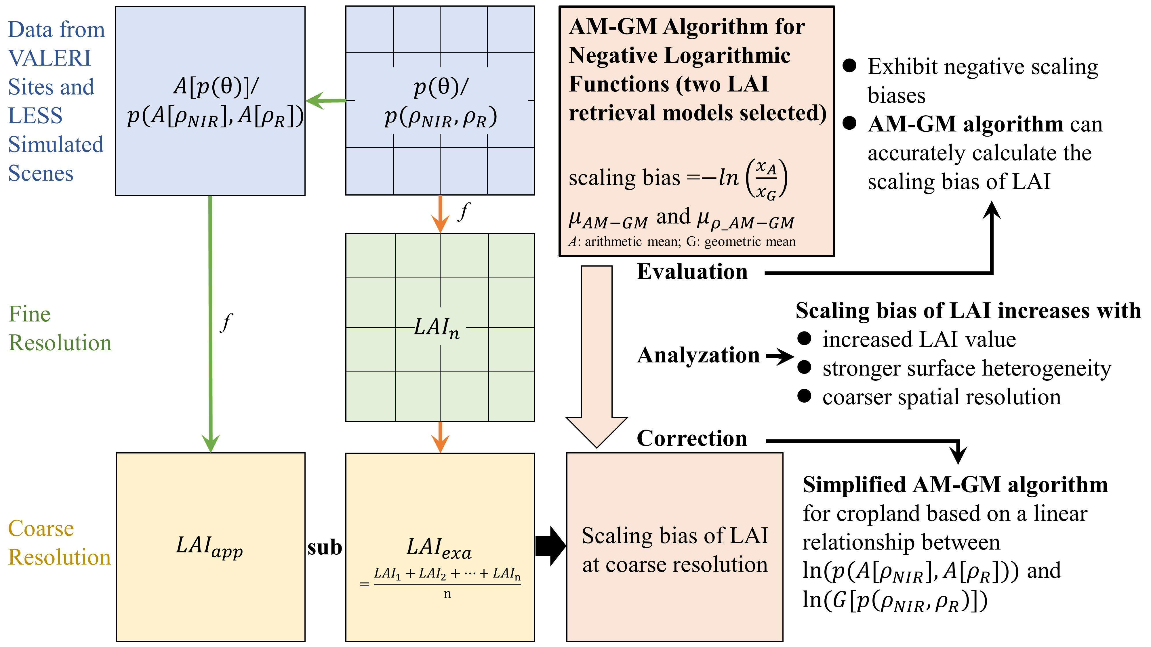
2.1. Simulated Data
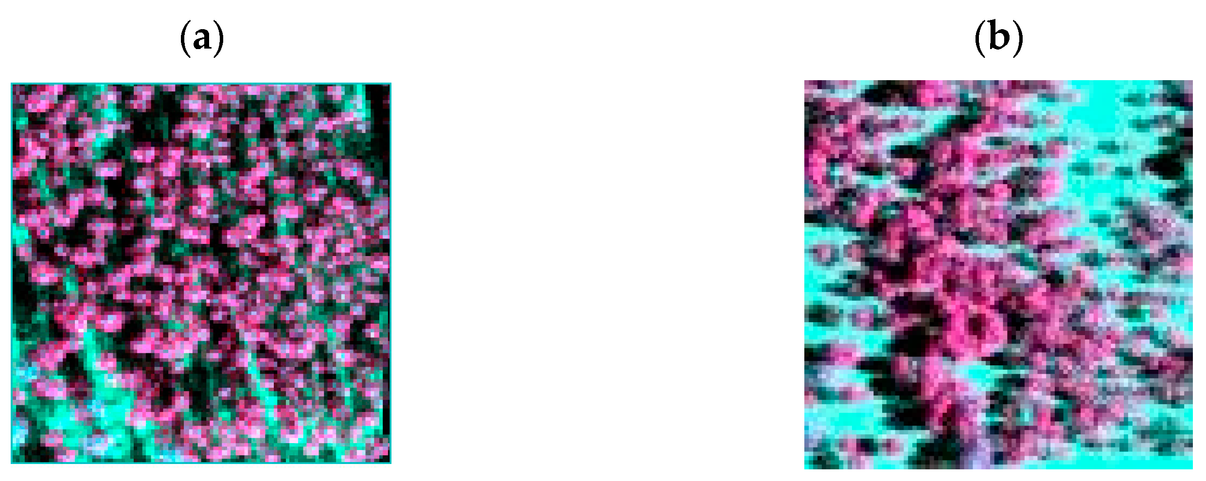
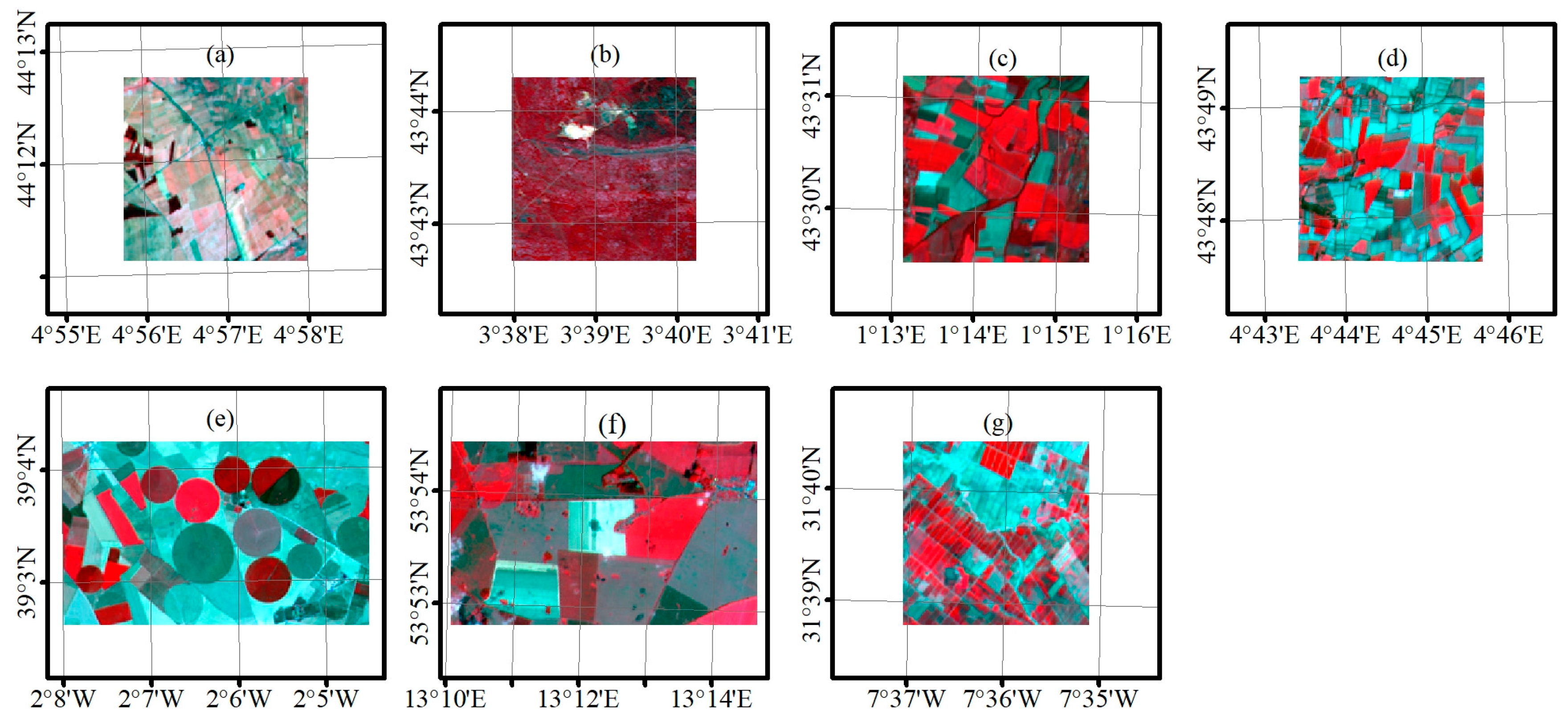
2.2. Site Data
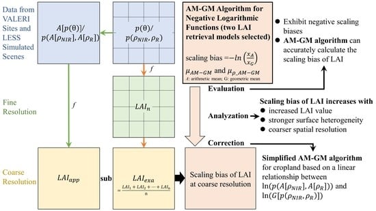
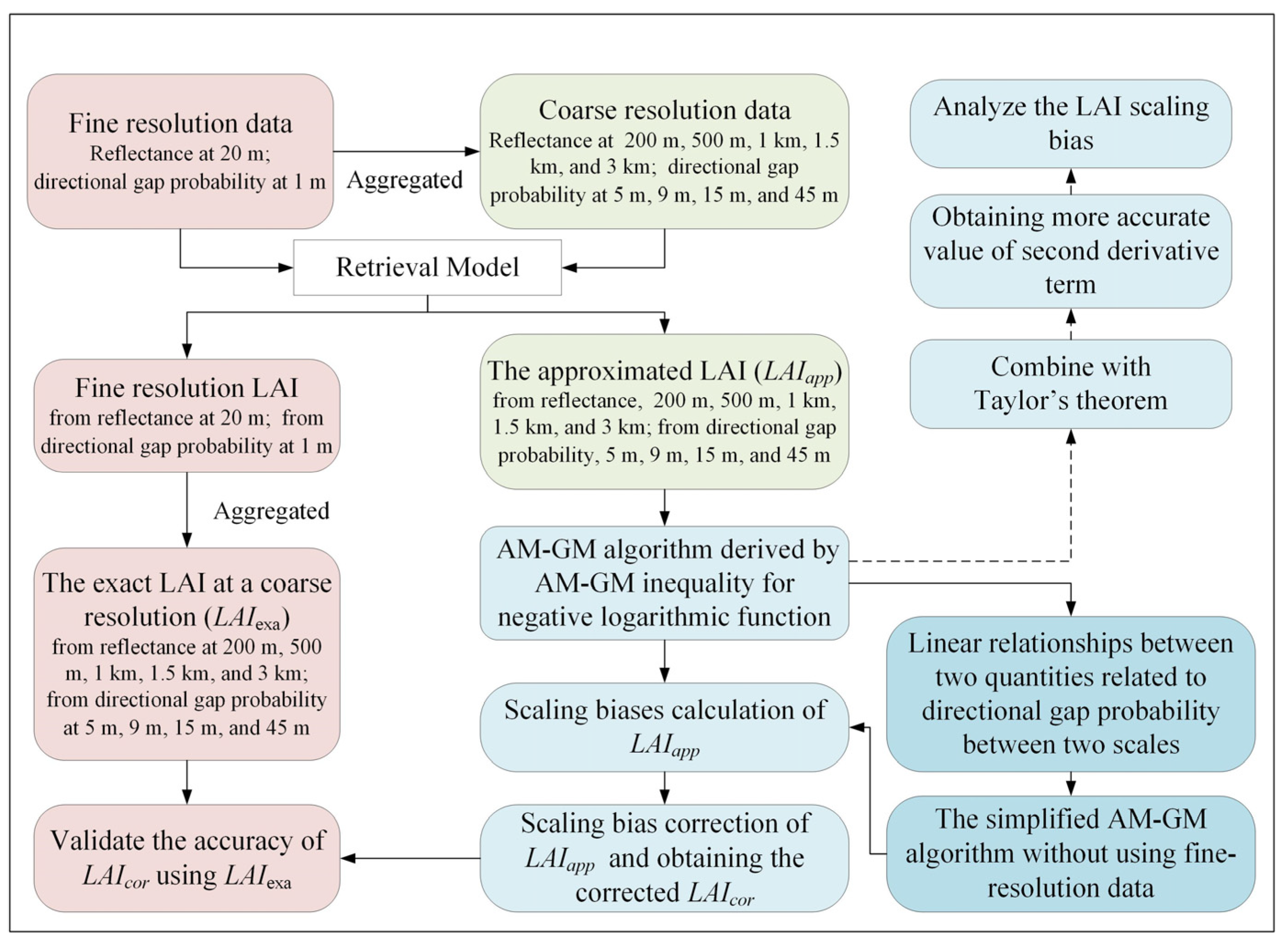
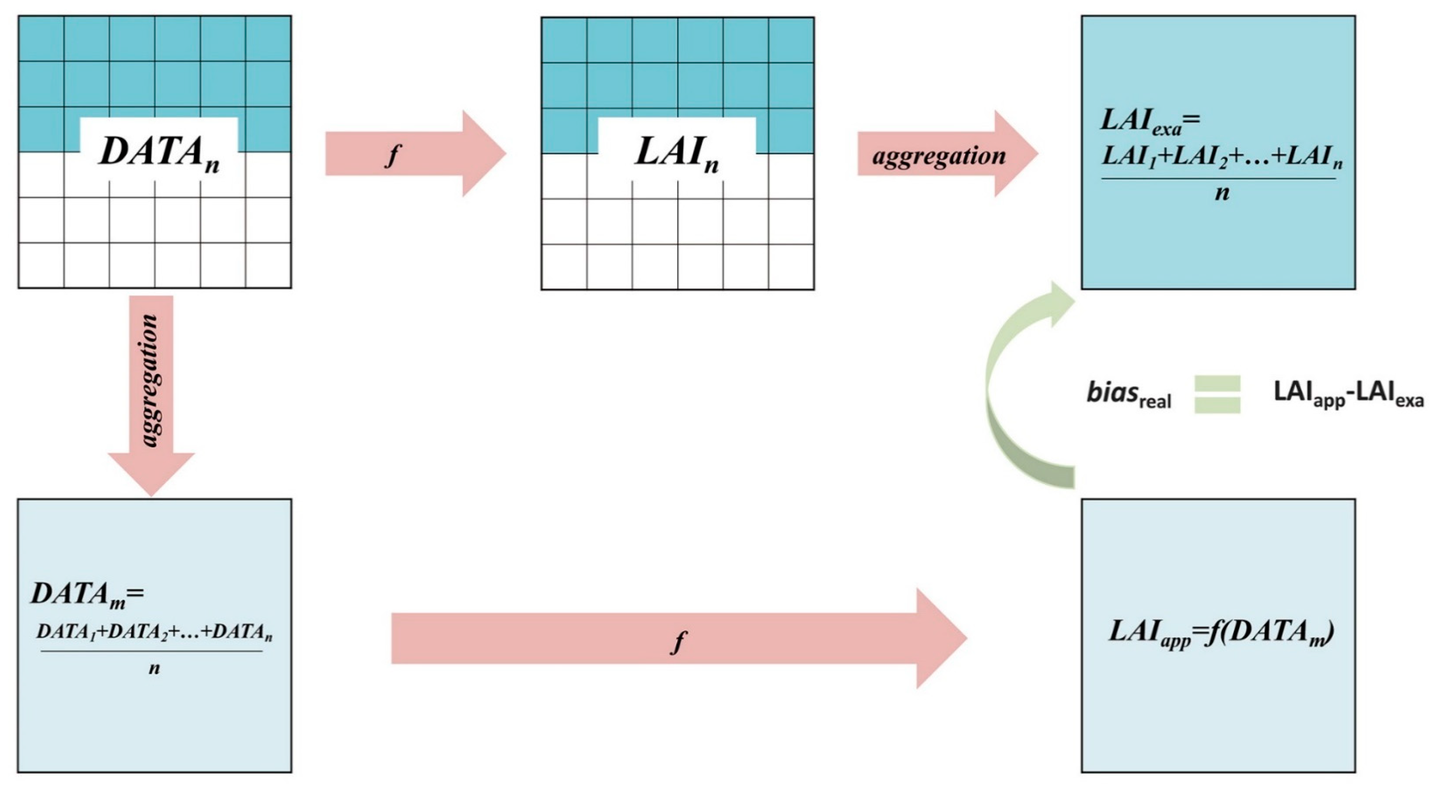
3. Methods
3.1. Mathematical Theory of the AM–GM Algorithm
3.1.1. Holder’s Defect and AM–GM Inequality
3.1.2. Calculation of LAI Scaling Bias
3.2. Calculate Factor μ
3.3. Simplify the AM–GM Algorithm
4. Results
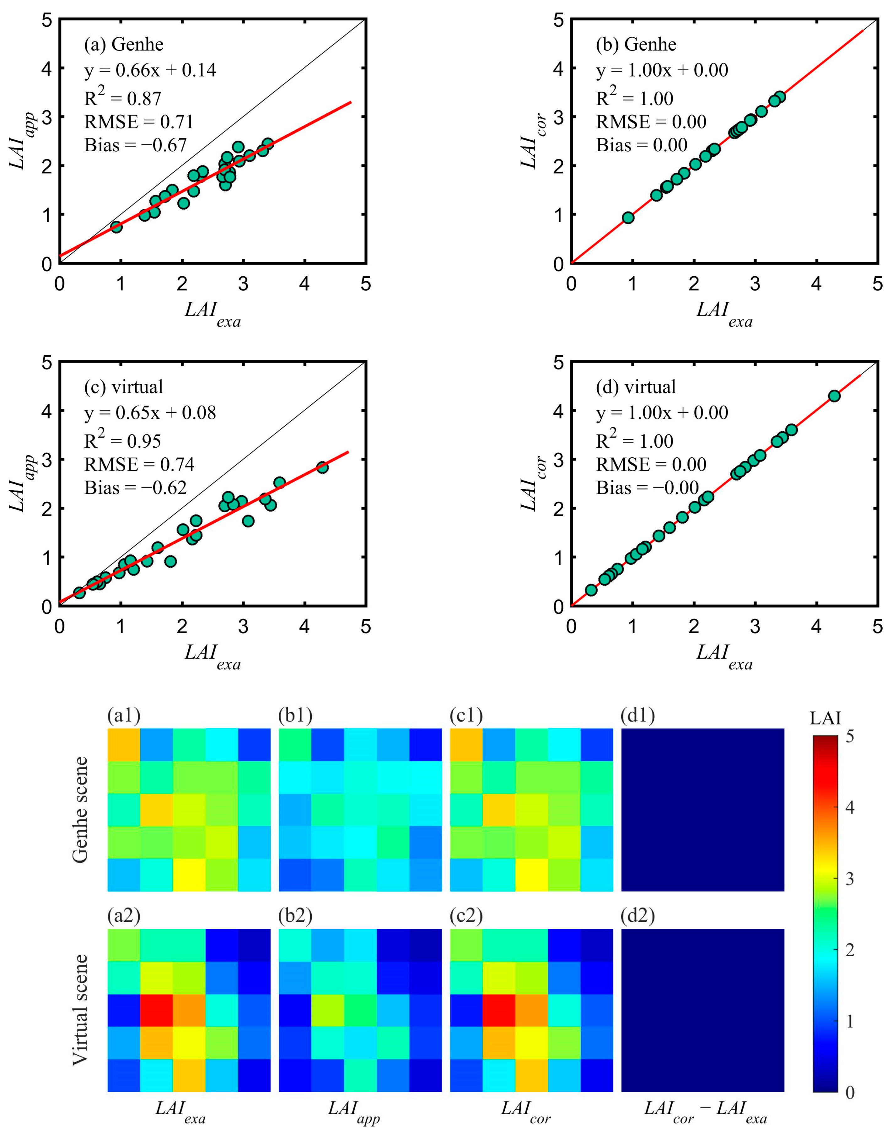
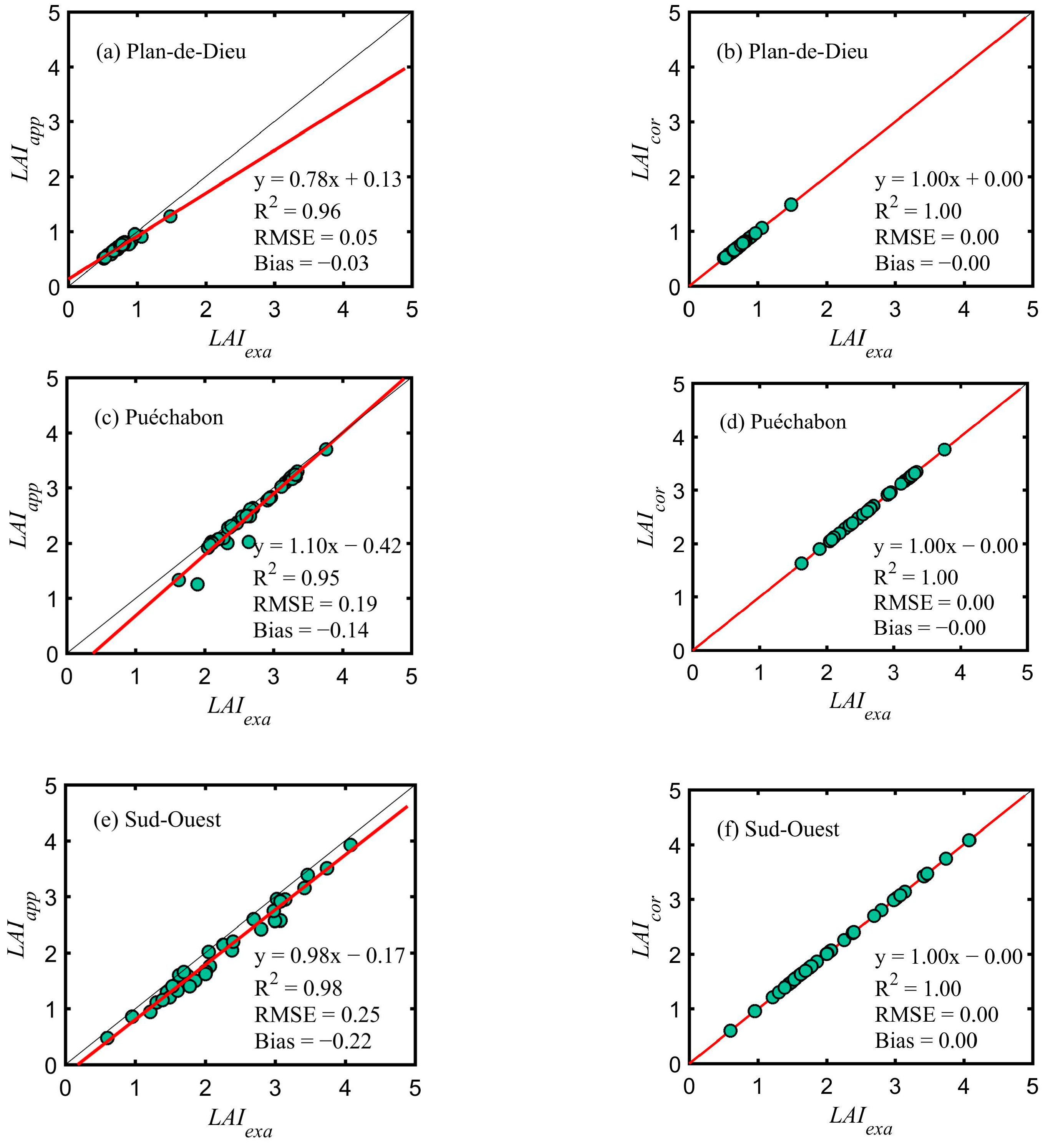
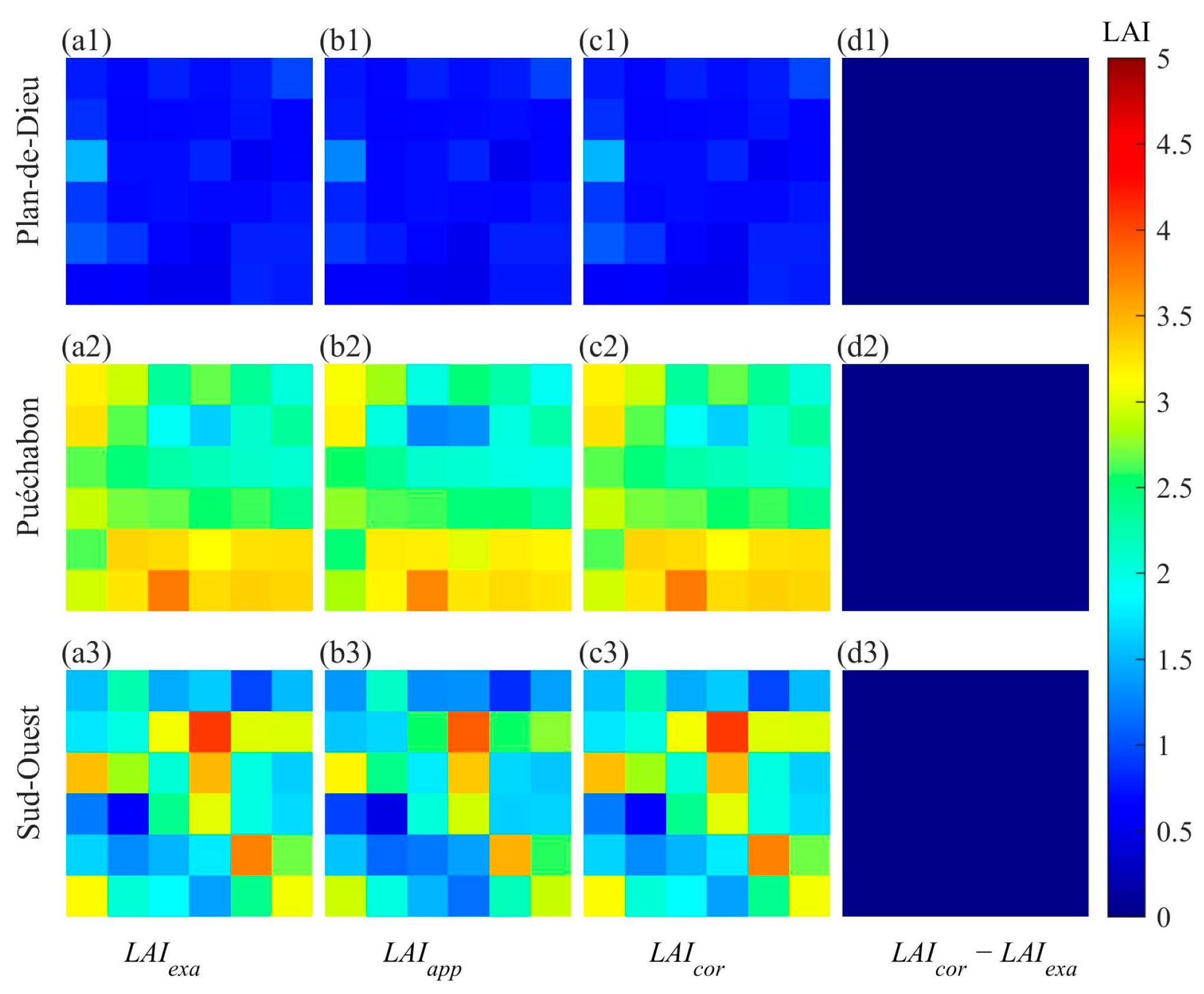
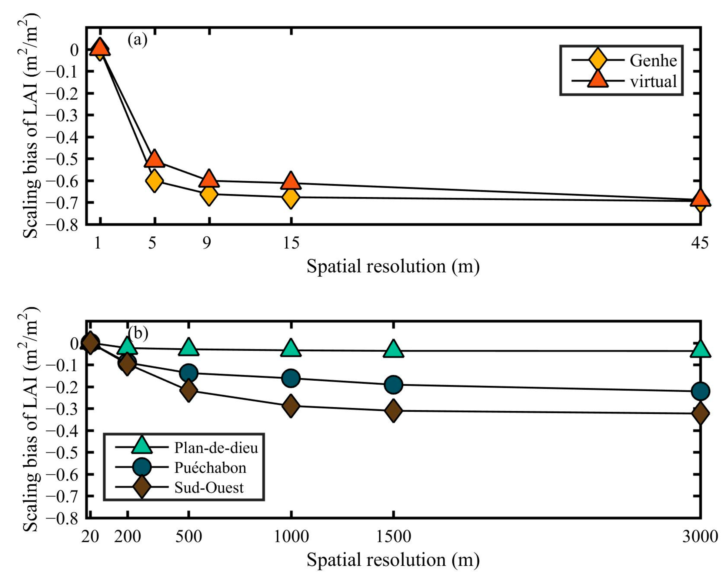
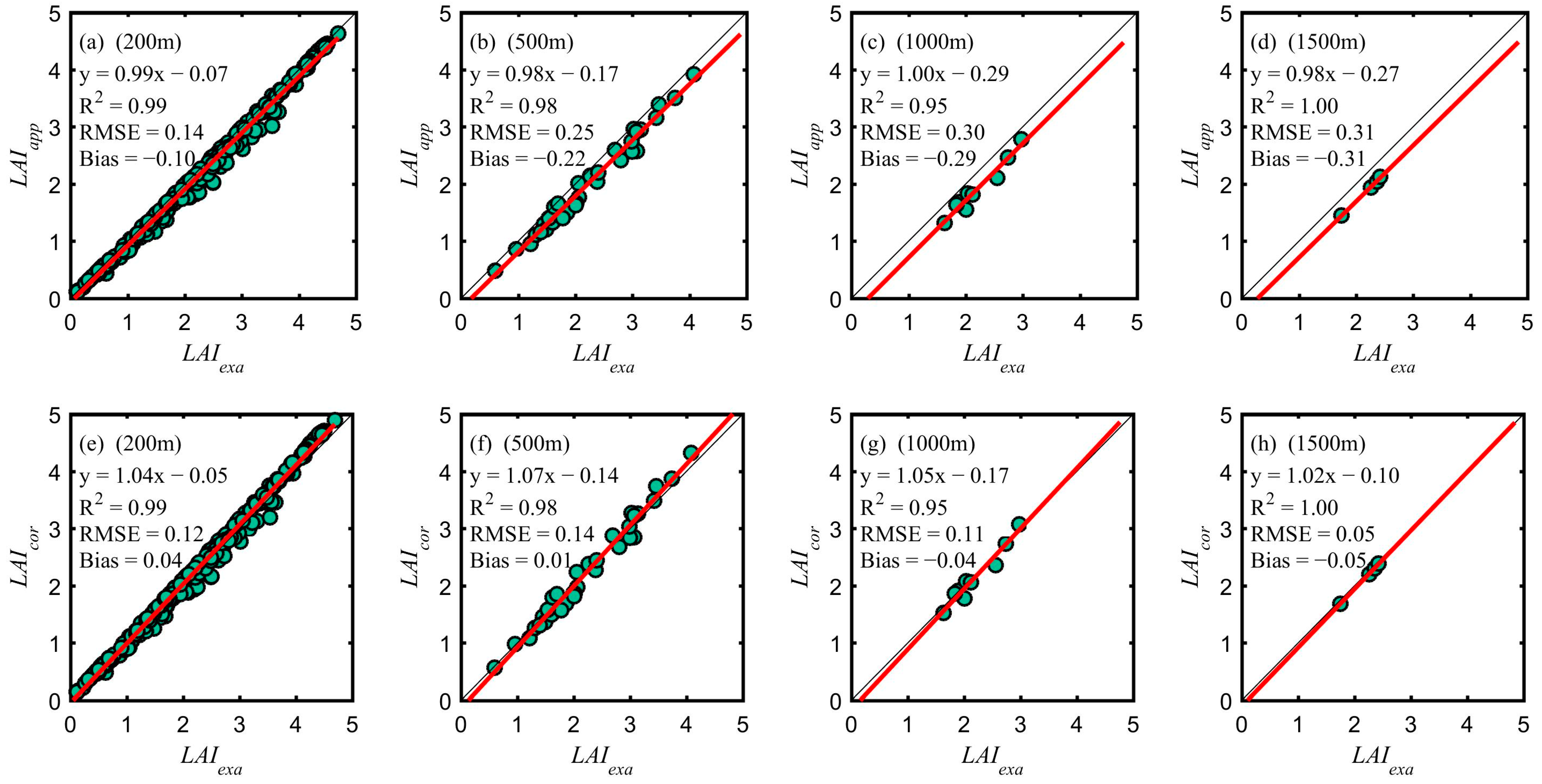
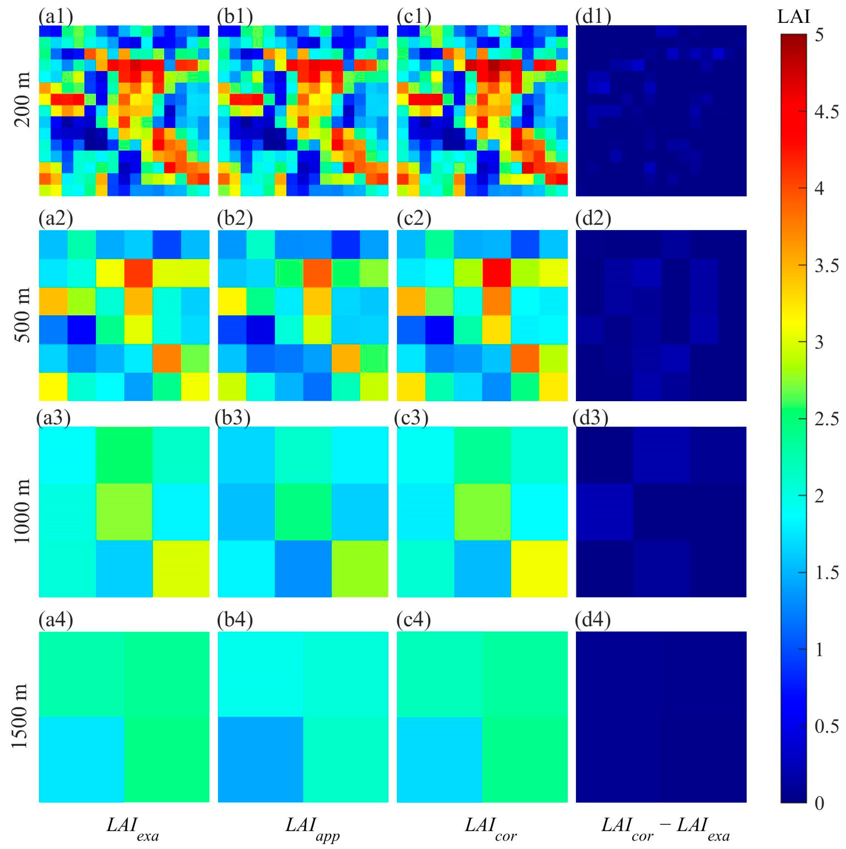
4.1. Validation Results of the AM–GM Algorithm
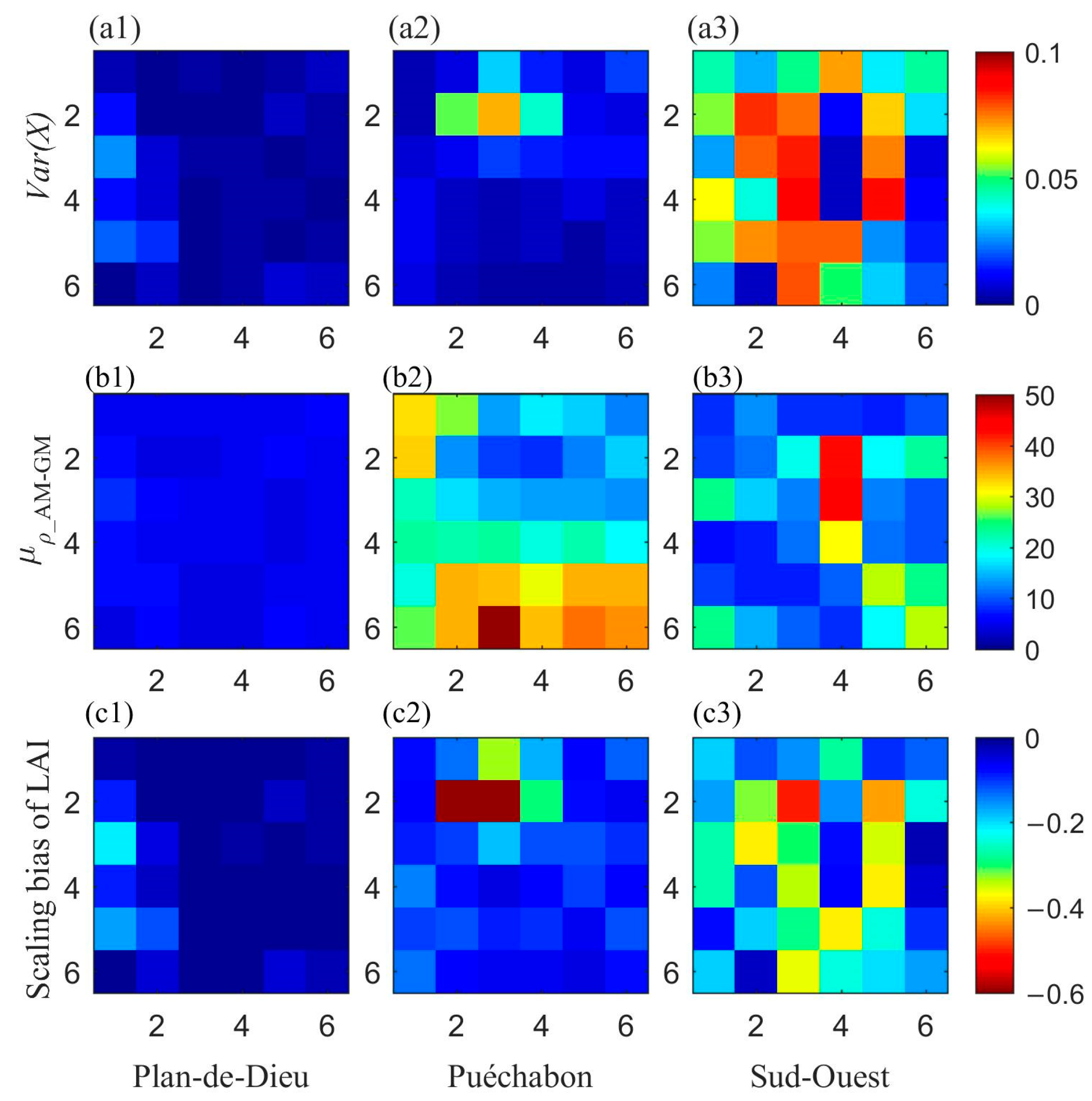
4.2. Analysis of LAI Scaling Bias
- Spatial resolution.
- Model nonlinearity.
- Surface heterogeneity.
4.3. Scaling Bias Calculated by the Simplified Algorithm
5. Discussion
5.1. Algorithm Comparison
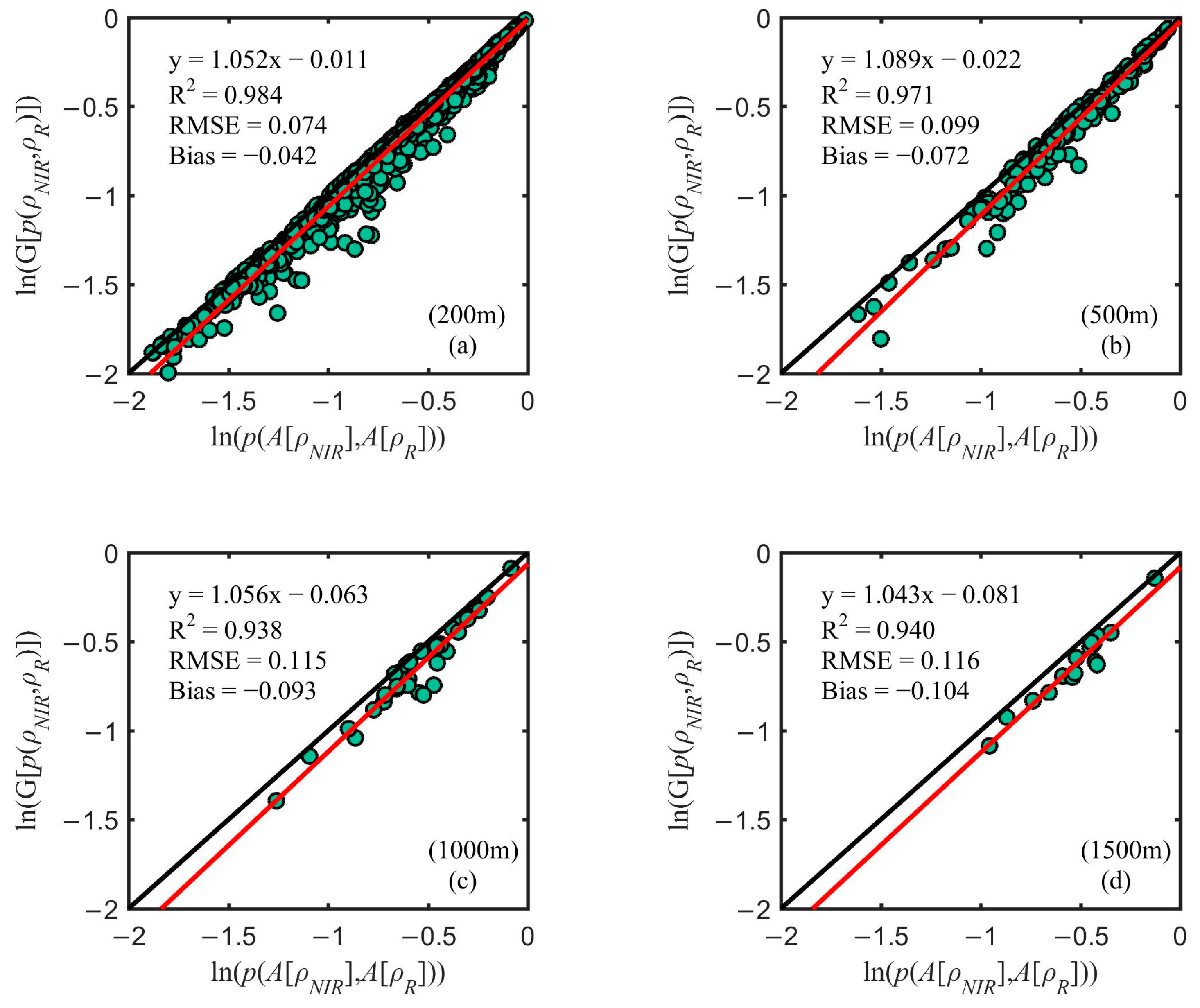
5.2. The Influence of NDVI Aggregation on the AM–GM Algorithm
5.3. Limitation of the AM–GM Algorithm
6. Conclusions
Author Contributions
Funding
Data Availability Statement
Acknowledgments
Conflicts of Interest
Appendix A
Appendix B
References
- Baret, F.; Weiss, M.; Lacaze, R.; Camacho, F.; Makhmara, H.; Pacholcyzk, P.; Smets, B. GEOV1: LAI and FAPAR essential climate variables and FCOVER global time series capitalizing over existing products. Part1: Principles of development and production. Remote Sens. Environ. 2013, 137, 299–309. [Google Scholar] [CrossRef]
- Wang, J.; Sun, R.; Zhang, H.; Xiao, Z.; Zhu, A.; Wang, M.; Yu, T.; Xiang, K. New Global MuSyQ GPP/NPP Remote Sensing Products From 1981 to 2018. IEEE J. Sel. Top. Appl. Earth Observ. Remote Sens. 2021, 14, 5596–5612. [Google Scholar] [CrossRef]
- Chen, Z.; Jia, K.; Wei, X.; Liu, Y.; Zhan, Y.; Xia, M.; Yao, Y.; Zhang, X. Improving leaf area index estimation accuracy of wheat by involving leaf chlorophyll content information. Comput. Electron. Agric. 2022, 196, 106902. [Google Scholar] [CrossRef]
- Cortés, J.; Mahecha, M.D.; Reichstein, M.; Myneni, R.B.; Chen, C.; Brenning, A. Where Are Global Vegetation Greening and Browning Trends Significant? Geophys. Res. Lett. 2021, 48, e2020GL091496. [Google Scholar] [CrossRef]
- Chen, C.; Park, T.; Wang, X.H.; Piao, S.L.; Xu, B.D.; Chaturvedi, R.K.; Fuchs, R.; Brovkin, V.; Ciais, P.; Fensholt, R.; et al. China and India lead in greening of the world through land-use management. Nat. Sustain. 2019, 2, 122–129. [Google Scholar] [CrossRef]
- Yu, T.; Zhang, Q.; Sun, R. Comparison of Machine Learning Methods to Up-Scale Gross Primary Production. Remote Sens. 2021, 13, 2448. [Google Scholar] [CrossRef]
- Chen, J.M.; Ju, W.M.; Ciais, P.; Viovy, N.; Liu, R.G.; Liu, Y.; Lu, X.H. Vegetation structural change since 1981 significantly enhanced the terrestrial carbon sink. Nat. Commun. 2019, 10, 4259. [Google Scholar] [CrossRef]
- Garrigues, S.; Allard, D.; Baret, F.; Weiss, M. Influence of the spatial heterogeneity on the non-linear estimation of Leaf Area Index from moderate resolution remote sensing data. Remote Sens. Environ. 2006, 105, 286–298. [Google Scholar] [CrossRef]
- Liu, W.H.; Shi, J.C.; Liang, S.L.; Zhou, S.G.; Cheng, J. Simultaneous retrieval of land surface temperature and emissivity from the FengYun-4A advanced geosynchronous radiation imager. Int. J. Digit. Earth 2022, 15, 198–225. [Google Scholar] [CrossRef]
- Wu, H.; Li, Z.-L. Scale Issues in Remote Sensing: A Review on Analysis, Processing and Modeling. Sensors 2009, 9, 1768–1793. [Google Scholar] [CrossRef]
- Zhang, J.; Wang, J.; Sun, R.; Zhou, H.; Zhang, H. A Model-Downscaling Method for Fine-Resolution LAI Estimation. Remote Sens. 2020, 12, 4147. [Google Scholar] [CrossRef]
- Deng, F.; Chen, J.M.; Plummer, S.; Chen, M.; Pisek, J. Algorithm for global leaf area index retrieval using satellite imagery. IEEE Trans. Geosci. Remote Sens. 2006, 44, 2219–2229. [Google Scholar] [CrossRef]
- Liang, S. Numerical experiments on the spatial scaling of land surface albedo and leaf area index. Remote Sens. Rev. 2000, 19, 225–242. [Google Scholar] [CrossRef]
- Tao, X.; Yan, B.; Wang, K.; Wu, D.; Fan, W.; Xu, X.; Liang, S. Scale transformation of Leaf Area Index product retrieved from multiresolution remotely sensed data: Analysis and case studies. Int. J. Remote Sens. 2009, 30, 5383–5395. [Google Scholar] [CrossRef]
- Yin, G.F.; Li, J.; Liu, Q.H.; Li, L.H.; Zeng, Y.L.; Xu, B.D.; Yang, L.; Zhao, J. Improving Leaf Area Index Retrieval Over Heterogeneous Surface by Integrating Textural and Contextual Information: A Case Study in the Heihe River Basin. IEEE Geosci. Remote Sens. Lett. 2015, 12, 359–363. [Google Scholar] [CrossRef]
- Xu, B.D.; Li, J.; Park, T.J.; Liu, Q.H.; Zeng, Y.L.; Yin, G.F.; Yan, K.; Chen, C.; Zhao, J.; Fan, W.L.; et al. Improving leaf area index retrieval over heterogeneous surface mixed with water. Remote Sens. Environ. 2020, 240, 111700. [Google Scholar] [CrossRef]
- Fang, H.; Baret, F.; Plummer, S.; Schaepman-Strub, G. An Overview of Global Leaf Area Index (LAI): Methods, Products, Validation, and Applications. Rev. Geophys. 2019, 57, 739–799. [Google Scholar] [CrossRef]
- Fisher, R.A.; Koven, C.D. Perspectives on the Future of Land Surface Models and the Challenges of Representing Complex Terrestrial Systems. J. Adv. Model. Earth Syst. 2020, 12, e2018MS001453. [Google Scholar] [CrossRef]
- Zhao, W.; Fan, W. Quantitative Representation of Spatial Heterogeneity in the LAI Scaling Transfer Process. IEEE Access 2021, 9, 83851–83862. [Google Scholar] [CrossRef]
- Jin, Z.; Tian, Q.; Chen, J.M.; Chen, M. Spatial scaling between leaf area index maps of different resolutions. J. Environ. Manag. 2007, 85, 628–637. [Google Scholar] [CrossRef]
- Raffy, M. Change of scale in models of remote sensing: A general method for spatialization of models. Remote Sens. Environ. 1992, 40, 101–112. [Google Scholar] [CrossRef]
- Hu, Z.; Islam, S. A framework for analyzing and designing scale invariant remote sensing algorithms. IEEE Trans. Geosci. Remote. Sens. 1997, 35, 747–755. [Google Scholar] [CrossRef]
- Jiang, J.; Liu, X.; Liu, C.; Wu, L.; Xia, X.; Liu, M.; Du, Z. Analyzing the Spatial Scaling Bias of Rice Leaf Area Index From Hyperspectral Data Using Wavelet-Fractal Technique. IEEE J. Sel. Top. Appl. Earth Observ. Remote Sens. 2015, 8, 3068–3080. [Google Scholar] [CrossRef]
- Wu, L.; Liu, X.; Qin, Q.; Zhao, B.; Ma, Y.; Liu, M.; Jiang, T. Scaling Correction of Remotely Sensed Leaf Area Index for Farmland Landscape Pattern With Multitype Spatial Heterogeneities Using Fractal Dimension and Contextural Parameters. IEEE J. Sel. Top. Appl. Earth Observ. Remote Sens. 2018, 11, 1472–1481. [Google Scholar] [CrossRef]
- Wu, L.; Qin, Q.; Liu, X.; Ren, H.; Wang, J.; Zheng, X.; Ye, X.; Sun, Y. Spatial Up-Scaling Correction for Leaf Area Index Based on the Fractal Theory. Remote Sens. 2016, 8, 197. [Google Scholar] [CrossRef]
- Chen, H.; Wu, H.; Li, Z.-L.; Tu, J. An Improved Computational Geometry Method for Obtaining Accurate Remotely Sensed Products via Convex Hulls With Dynamic Weights: A Case Study With Leaf Area Index. IEEE J. Sel. Top. Appl. Earth Observ. Remote Sens. 2019, 12, 2308–2319. [Google Scholar] [CrossRef]
- Wang, J.P.; Wu, X.D.; Wen, J.G.; Xiao, Q.; Gong, B.C.; Ma, D.J.; Cui, Y.R.; Lin, X.W.; Bao, Y.F. Upscaling in Situ Site-Based Albedo Using Machine Learning Models: Main Controlling Factors on Results. IEEE Trans. Geosci. Remote Sens. 2022, 60, 3095153. [Google Scholar] [CrossRef]
- Wu, X.D.; Wen, J.G.; Tang, R.Q.; Wang, J.P.; Zeng, Q.C.; Li, Z.; You, D.Q.; Lin, X.W.; Gong, B.C.; Xiao, Q. Quantification of the uncertainty in multiscale validation of coarse-resolution satellite albedo products: A study based on airborne CASI data. Remote Sens. Environ. 2023, 287, 113465. [Google Scholar] [CrossRef]
- Chen, Y.G. Fractal Modeling and Fractal Dimension Description of Urban Morphology. Entropy 2020, 22, 961. [Google Scholar] [CrossRef]
- Jiang, J.; Ji, X.; Yao, X.; Tian, Y.; Zhu, Y.; Cao, W.; Cheng, T. Evaluation of Three Techniques for Correcting the Spatial Scaling Bias of Leaf Area Index. Remote Sens. 2018, 10, 221. [Google Scholar] [CrossRef]
- Becker, R. The Variance Drain and Jensen’s Inequality. CAEPR Work. Pap. 2012, 2004–2012. [Google Scholar] [CrossRef]
- Li, W.; Mu, X. Using fractal dimension to correct clumping effect in leaf area index measurement by digital cover photography. Agric. For. Meteorol. 2021, 311, 108695. [Google Scholar] [CrossRef]
- Shi, Y.; Wang, J.; Wang, J.; Qu, Y. A Prior Knowledge-Based Method to Derivate High-Resolution Leaf Area Index Maps with Limited Field Measurements. Remote Sens. 2017, 9, 13. [Google Scholar] [CrossRef]
- Zhang, X.; Yan, G.; Li, Q.; Li, Z.-L.; Wan, H.; Guo, L. Evaluating the fraction of vegetation cover based on NDVI spatial scale correction model. Int. J. Remote Sens. 2006, 27, 5359–5372. [Google Scholar] [CrossRef]
- Qi, J.; Xie, D.; Yin, T.; Yan, G.; Gastellu-Etchegorry, J.; Li, L.; Zhang, W.; Mu, X.; Norford, L. LESS: LargE-Scale remote sensing data and image simulation framework over heterogeneous 3D scenes. Remote Sens. Environ. 2019, 221, 695–706. [Google Scholar] [CrossRef]
- Xu, Y.; Xie, D.; Qi, J.; Yan, G.; Mu, X.; Zhang, W. Influence of woody elements on nadir reflectance of forest canopy based on simulations by using the LESS model. J. Remote Sens. 2021, 25, 1138–1151. [Google Scholar]
- Nilson, T. A theoretical analysis of frequency of gaps in plant stands. Agric. Meteorol. 1971, 8, 25. [Google Scholar] [CrossRef]
- Wang, W.-M.; Li, Z.-L.; Su, H.-B. Comparison of leaf angle distribution functions: Effects on extinction coefficient and fraction of sunlit foliage. Agric. For. Meteorol. 2007, 143, 106–122. [Google Scholar] [CrossRef]
- Yan, G.; Hu, R.; Luo, J.; Weiss, M.; Jiang, H.; Mu, X.; Xie, D.; Zhang, W. Review of indirect optical measurements of leaf area index: Recent advances, challenges, and perspectives. Agric. For. Meteorol. 2019, 265, 390–411. [Google Scholar] [CrossRef]
- Xiao, Z.; Liang, S.; Wang, J.; Chen, P.; Yin, X.; Zhang, L.; Song, J. Use of General Regression Neural Networks for Generating the GLASS Leaf Area Index Product From Time-Series MODIS Surface Reflectance. IEEE Trans. Geosci. Remote Sens. 2014, 52, 209–223. [Google Scholar] [CrossRef]
- Fang, H. Canopy clumping index (CI): A review of methods, characteristics, and applications. Agric. For. Meteorol. 2021, 303, 18. [Google Scholar] [CrossRef]
- Ryu, Y.; Nilson, T.; Kobayashi, H.; Sonnentag, O.; Law, B.E.; Baldocchi, D.D. On the correct estimation of effective leaf area index: Does it reveal information on clumping effects? Agric. For. Meteorol. 2010, 150, 463–472. [Google Scholar] [CrossRef]
- Tang, S.; Chen, J.; Zhu, Q.; Li, X.; Chen, M.; Sun, R.; Zhou, Y.; Deng, F.; Xie, D. LAI inversion algorithm based on directional reflectance kernels. J. Environ. Manag. 2007, 85, 638–648. [Google Scholar] [CrossRef]
- Baret, F.; Guyot, G. Potentials and limits of vegetation indices for LAI and APAR assessment. Remote Sens. Environ. 1991, 35, 161–173. [Google Scholar] [CrossRef]
- Chen, J.M.; Menges, C.H.; Leblanc, S.G. Global mapping of foliage clumping index using multi-angular satellite data. Remote Sens. Environ. 2005, 97, 447–457. [Google Scholar] [CrossRef]
- Ma, L.; Li, C.; Tang, B.; Tang, L.; Bi, Y.; Zhou, B.; Li, Z.-L. Impact of spatial LAI heterogeneity on estimate of directional gap fraction from SPOT-satellite data. Sensors 2008, 8, 3767–3779. [Google Scholar] [CrossRef]


| Sensor | Parameter Value | Optical Database | Parameter Value |
|---|---|---|---|
| Type | Orthographic | Larch Branch | Ground Measurements |
| Width (pixels) | 45 | Brown Loam | Ground Measurements |
| Height (pixels) | 45 | Larch Leaf | Ground Measurements |
| Samples (/pixel) | 64 | Terrain | Parameter Value |
| Spectral Bands | 482:60, 561.5:57, 654.5:37, 865:28 | Type | Plane |
| Image Format | Spectrum | XSize (m) | 45 |
| NoData Value | −1 | YSize (m) | 45 |
| Width Extent (m) | 45 | BRDF Type | Lambertian |
| Height Extent (m) | 45 | Optical Property | Brown Loam |
| Four Components Product | Tick | ||
| Observation | Parameter Value | Objects | Parameter Value |
| View Zenith (°) | 0 | Single-Tree Models of Larch | Constructed by Xu et al. [36] |
| View Azimuth (°) | 180 | ||
| Sensor Height (m) | 30 | ||
| Illumination and Atmosphere | Parameter Value | Advanced | Parameter Value |
| Sun Zenith (°) | 30 | Minimum Iterations | 5 |
| Sun Azimuth (°) | 90 | Number of Cores | 20 |
| Sky-Type | SKY_TO_TOTAL | ||
| Sky-Percentage | 0, 0 |
| Site Name | Land Cover | Day of Year | Image Year | Spatial Resolution | Site Size | Location |
|---|---|---|---|---|---|---|
| Plan-de-Dieu | Crops | 181 | 2004 | 20 m | 3 km × 3 km | 44°11′N, 4°56′E |
| Puéchabon | Mediterranean Forests | 163 | 2001 | 20 m | 3 km × 3 km | 43°43′N, 3°38′E |
| Sud-Ouest | Nine Crops | 201 | 2002 | 20 m | 3 km × 3 km | 43°30′N, 1°14′E |
| Les Alpilles | Crops | 204 | 2002 | 20 m | 3 km × 3 km | 43°48′N, 4°42′W |
| Barrax | Crops | 195 | 2003 | 20 m | 5 km × 3 km | 39°40′N, 2°60′W |
| Demmin | Crops | 164 | 2004 | 20 m | 5 km × 3 km | 53°53′N, 13°12′E |
| Haouz | Crops | 73 | 2003 | 20 m | 3 km × 3 km | 31°39′N, 7°36′W |
| Site Name | Before Correction | After Correction | ||
|---|---|---|---|---|
| RMSE | Bias | RMSE | Bias | |
| Genhe | 0.71 | −0.67 | 0.00 | 0.00 |
| Virtual | 0.74 | −0.62 | 0.00 | 0.00 |
| Plan-de-Dieu | 0.05 | −0.03 | 0.00 | 0.00 |
| Puéchabon | 0.19 | −0.14 | 0.00 | 0.00 |
| Sud-Ouest | 0.25 | −0.22 | 0.00 | 0.00 |
| Spatial Resolution | 200 m | 500 m | 1000 m | 1500 m | |
|---|---|---|---|---|---|
| Parameters | |||||
| 0.052 | 0.089 | 0.056 | 0.043 | ||
| 0.011 | 0.022 | 0.063 | 0.081 | ||
| Site Name | Input Variable | |||
|---|---|---|---|---|
| RMSE | Bias | RMSE | Bias | |
| Plan-de-Dieu | 5.56 | −3.99 | 0.01 | −0.00 |
| Puéchabon | 5.48 | −4.58 | 0.02 | −0.01 |
| Sud-Ouest | 13.43 | 7.16 | 0.02 | 0.01 |
| Site Name | Considering the Scaling Bias of NDVI | Ignoring the Scaling Bias of NDVI | ||
|---|---|---|---|---|
| RMSE | Bias | RMSE | Bias | |
| Plan-de-Dieu | 0.00 | 0.00 | 0.18 | 0.01 |
| Puéchabon | 0.00 | 0.00 | 0.49 | 0.04 |
| Sud-Ouest | 0.00 | 0.00 | 0.61 | −0.08 |
Disclaimer/Publisher’s Note: The statements, opinions and data contained in all publications are solely those of the individual author(s) and contributor(s) and not of MDPI and/or the editor(s). MDPI and/or the editor(s) disclaim responsibility for any injury to people or property resulting from any ideas, methods, instructions or products referred to in the content. |
© 2023 by the authors. Licensee MDPI, Basel, Switzerland. This article is an open access article distributed under the terms and conditions of the Creative Commons Attribution (CC BY) license (https://creativecommons.org/licenses/by/4.0/).
Share and Cite
Zhang, J.; Sun, R.; Xiao, Z.; Zhao, L.; Xie, D. AM–GM Algorithm for Evaluating, Analyzing, and Correcting the Spatial Scaling Bias of the Leaf Area Index. Remote Sens. 2023, 15, 3068. https://doi.org/10.3390/rs15123068
Zhang J, Sun R, Xiao Z, Zhao L, Xie D. AM–GM Algorithm for Evaluating, Analyzing, and Correcting the Spatial Scaling Bias of the Leaf Area Index. Remote Sensing. 2023; 15(12):3068. https://doi.org/10.3390/rs15123068
Chicago/Turabian StyleZhang, Jingyu, Rui Sun, Zhiqiang Xiao, Liang Zhao, and Donghui Xie. 2023. "AM–GM Algorithm for Evaluating, Analyzing, and Correcting the Spatial Scaling Bias of the Leaf Area Index" Remote Sensing 15, no. 12: 3068. https://doi.org/10.3390/rs15123068
APA StyleZhang, J., Sun, R., Xiao, Z., Zhao, L., & Xie, D. (2023). AM–GM Algorithm for Evaluating, Analyzing, and Correcting the Spatial Scaling Bias of the Leaf Area Index. Remote Sensing, 15(12), 3068. https://doi.org/10.3390/rs15123068