1. Introduction
The arable areas, containing regularly harvested crops and pastures per unit area, are a key indicator of Sustainable Development Goal 2 [
1]. Closing the yield gap and increasing agricultural resource use efficiency help to achieve global food security. Arable field areas are a key input to crop yield models that inform these activities. However, remote sensing-based estimates of arable areas in smallholder farming systems do not achieve the level of accuracy needed for effective decision-making for four reasons [
2]. First, it is challenging to spectrally resolve the small (<2 ha) and irregularly shaped fields [
3] because of spectral similarities with natural vegetation and lack of incorporation of contextual information. Second, persistent cloud cover frequently obscures the target under study [
4]. Third, the diversity of farming practices causes large differences in crop calendars and phenology at the pixel level [
5]. Lastly, there is a lack of high-quality (spatially and temporally) labeled sample sets for model training and testing [
6].
Several methodological steps can be taken to overcome these difficulties. The first is related to image selection. High-resolution (≤5 m) commercial satellites can capture small fields, but the imagery is costly [
7], which has limited their use for regional or global studies [
8]. On the other hand, analysis-ready moderate-resolution (~30 m) remote satellite images are freely available in cloud-computing environments such as Google Earth Engine (GEE) [
9]. The Landsat missions, which began in 1972, have long been used for arable field mapping because they provide a moderate resolution, multi-decadal record of observations. In comparison, the Sentinel-2 constellation (a + b) was launched in 2015. It has several advantages over the Landsat missions, including higher spatial resolution (10–20 m versus 30 m), higher return frequency (5 days versus 16 days), and four additional narrow bands (≤20 nm) in the red-edge and near-infrared (NIR). The narrow bands are more sensitive to changes in crop status than the broader red and NIR bands available from traditional multispectral broadband sensors [
10]. The high frequency and spatial-spectral resolution of Sentinel-2 have been exploited in some studies for arable field mapping using image segmentation [
11] and crop phenological metrics [
12]. Similarly, Sentinel-1 SAR (synthetic-aperture radar) data, which has been available since 2014, is increasingly used to study vegetation dynamics because it is almost unaffected by cloud cover or haze [
13]. Sentinel-1 delivers co- and cross-polarizations of SAR backscatter (i.e., VV and VH, or HH and HV), which are sensitive to canopy structural properties and moisture status. Thus, integrating moderate-resolution optical Sentinel-2 and Sentinel-1 data can improve the spectral separability of croplands from other land cover types while minimizing the impact of cloud cover in the sub-Saharan region [
14].
Including image features incorporating spatial context into machine learning models for fragmented landscapes can improve arable area mapping [
15]. Image texture features represent one such approach, as they capture the contextuality of landcover types by measuring pixel intensity variation relative to neighboring pixels. This approach has the added benefit of reducing the signal-to-noise ratio at the individual pixel level and improving the ability to capture vegetation exhibiting similar spectral reflectance. For instance, crop areas may appear smoother than shrubland at a higher spatial resolution (~1 m) [
16]. Previous research by Debats [
7] demonstrated the importance of texture features over spectral features for arable field mapping at a higher spatial scale. However, most existing studies for sub-Saharan Africa are focused on high spatial resolution texture features [
7,
17]. Conversely, this study comprehensively explores the use of moderate-resolution texture features in the sub-Saharan region.
Another approach that can be used to improve the performance of mapping models is image stratification, which involves clustering geospatial data into common landscape patterns [
18]. Previous studies [
6,
7,
14,
19] have used fixed season features to map arable fields, which do not account for the diversity in crop calendars in sub-Saharan Africa. To accurately map vegetation seasonality, it is imperative to obtain long-term records spanning multiple decades to minimize the influence of year-to-year variations in weather and environmental conditions. Daily records of the Normalized Difference Vegetation Index (NDVI) at lower spatial resolution images (MODIS or PROBA-V) can be utilized to delineate landscape strata by image stratification [
20]. These strata account for differences in farming practices and provide a robust means of characterizing vegetation seasonality per-pixel basis. For example, Mohammed [
21] generated 1 km field fractions in Ethiopia using a similar procedure. They included slope, elevation, and Landsat-8 (OLI) NDVI composites at 30 m resolution on top of PROBA-V in the model to improve the separability of croplands from natural vegetation showing similar phenology. Both studies found that disaggregated statistics using landscape strata is an important image predictor to map arable field fractions at coarser resolution. Considering this prior knowledge, this study also explores landscape strata to map distinct pixel-level vegetation seasonality and to disaggregate district-level statistics (as one of the model predictors).
Dense, high-quality training and reference samples are other key methodological requirements for developing accurate mapping models [
22]. Machine learning models require a large sample size for training and testing and can be particularly sensitive to label errors [
6,
22]. Geo-tagging of arable fields annually is impractical and resource-intensive, especially in sub-Saharan Africa, while the small field sizes and their high temporal variability make collecting labels by annotating fields in available high-resolution imagery, typically those contained in virtual globe base maps, problematic because of the temporal mismatches between the labeled imagery and that being classified [
6]. To overcome this challenge, labels collected on the new high spatial resolution (<5 m), daily imagery provided by the PlanetScope (PS) sensor [
23], together with rigorous quality checks can help to provide large numbers of temporally consistent samples, which in turn enable more accurate mapping models to be developed [
6]. In this research, the process of ensuring quality is referred to as cross-checking consensus PS labels, which is performed by experts in the field, and is further discussed in
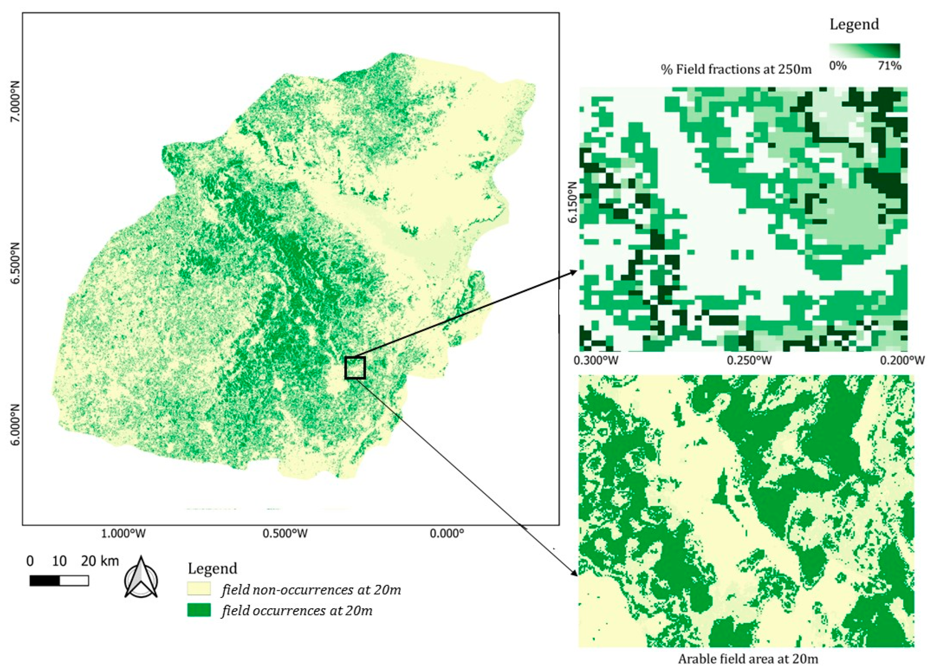
Section 3.5. Given the scope of the improvements mentioned, this study aims to map arable fields at 20 m spatial resolution (at red-edge band resolution level) within complex smallholder-dominated agricultural systems in the Eastern region of Ghana by an innovative combination of Sentinel-1, Sentinel-2, MODIS NDVI strata, and PS based dense network of labeled training data (labeler (Repo:
https://github.com/agroimpacts/labeller (accessed on 26 August 2019)) module developed by Agricultural Mapping Platform) to develop a machine learning-based mapping algorithm. The proposed approach uniquely uses high-temporal MODIS NDVI strata to map crop calendars and uses it to stratify cloud-free finer spatial resolution Sentinel image features. The study analyzed S2 spectral features to exploit narrowband red-edge and SWIR channels for better separation of cropland from natural vegetation and S1 polarimetric image features for capturing surface roughness to separate cropland from other landcover classes using frequent cloud-free observations. It also utilizes combined S1 + S2 textural features to capture small fragmented crop areas, and topographical features to capture landscape-level crop distribution providing comprehensive insights into multi-sensor image features predicting arable area. The study provides insight into the multi-sensor approach for arable area mapping.
2. Study Area
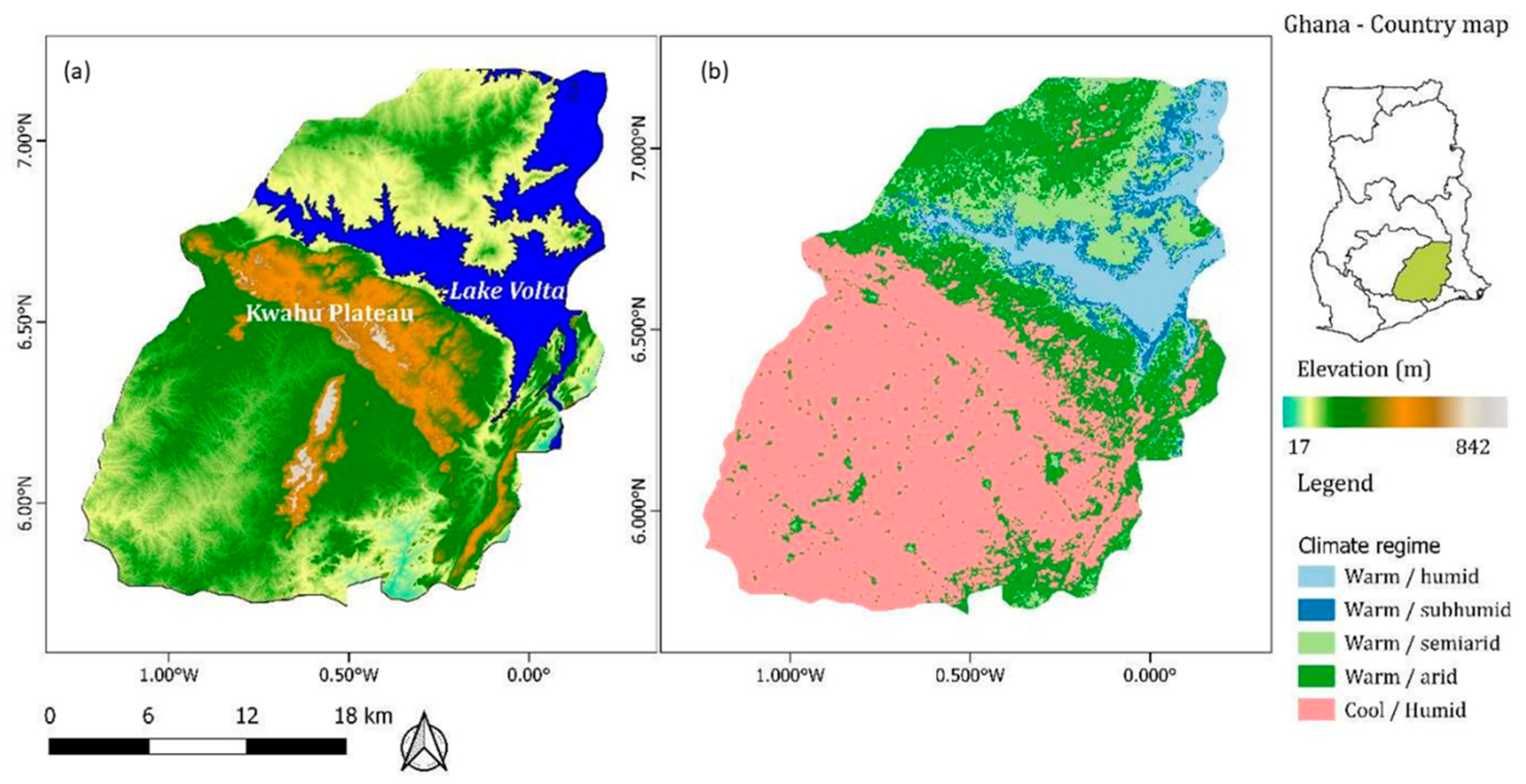
The study area, the Eastern Region of Ghana, spans an area of 19,000 km
2 in the southeast of the country (
Figure 1). The average annual temperature ranges from 22 °C to 31 °C with an annual rainfall of 111 mm. By area, 42%, 55%, and 3% of the region are under maize, cassava, and rice cultivation, respectively [
24].
The region is topographically complex and contains rainfed and irrigated agricultural fields (
Figure 1). The Kwahu Plateau separates the Afram plains in the north from the rest of the region. The north’s Afram plains are low-lying areas with an elevation <17 m whereas the south region has hilly areas with an elevation of 200–300 m. The fields are drier in the Afram plains compared to the south because they are on the leeward side of the Kwahu Plateau [
25]. The main rainy season (April to July) is triggered by the West African Monsoon and the northward ascent of the Intertropical Convergence Zone (ITCZ). Both regions have one major dry season from November to March and a minor dry season from July to August. Arable fields in the Afram plains are sparser and irrigated by Lake Volta during the minor dry season, which prolongs the growing season. The main crops grown in the plains are yam, maize, and vegetables. Areas south of the plains receive considerably more rainfall, so the fields are exclusively rainfed and more intensely cultivated. In the south, agroforestry is widely practiced as well. The fields typically consist of cocoa and oil palm mix intercropped with cassava, rice, and maize.
Figure 1.
The eastern region of Ghana: (
a) topography (SRTM DEM at 30 m), (
b) major climate zones based on temperature and rainfall, adopted from Bessah [
26] and remapped using landscape strata of the study.
Figure 1.
The eastern region of Ghana: (
a) topography (SRTM DEM at 30 m), (
b) major climate zones based on temperature and rainfall, adopted from Bessah [
26] and remapped using landscape strata of the study.
3. Data and Methods
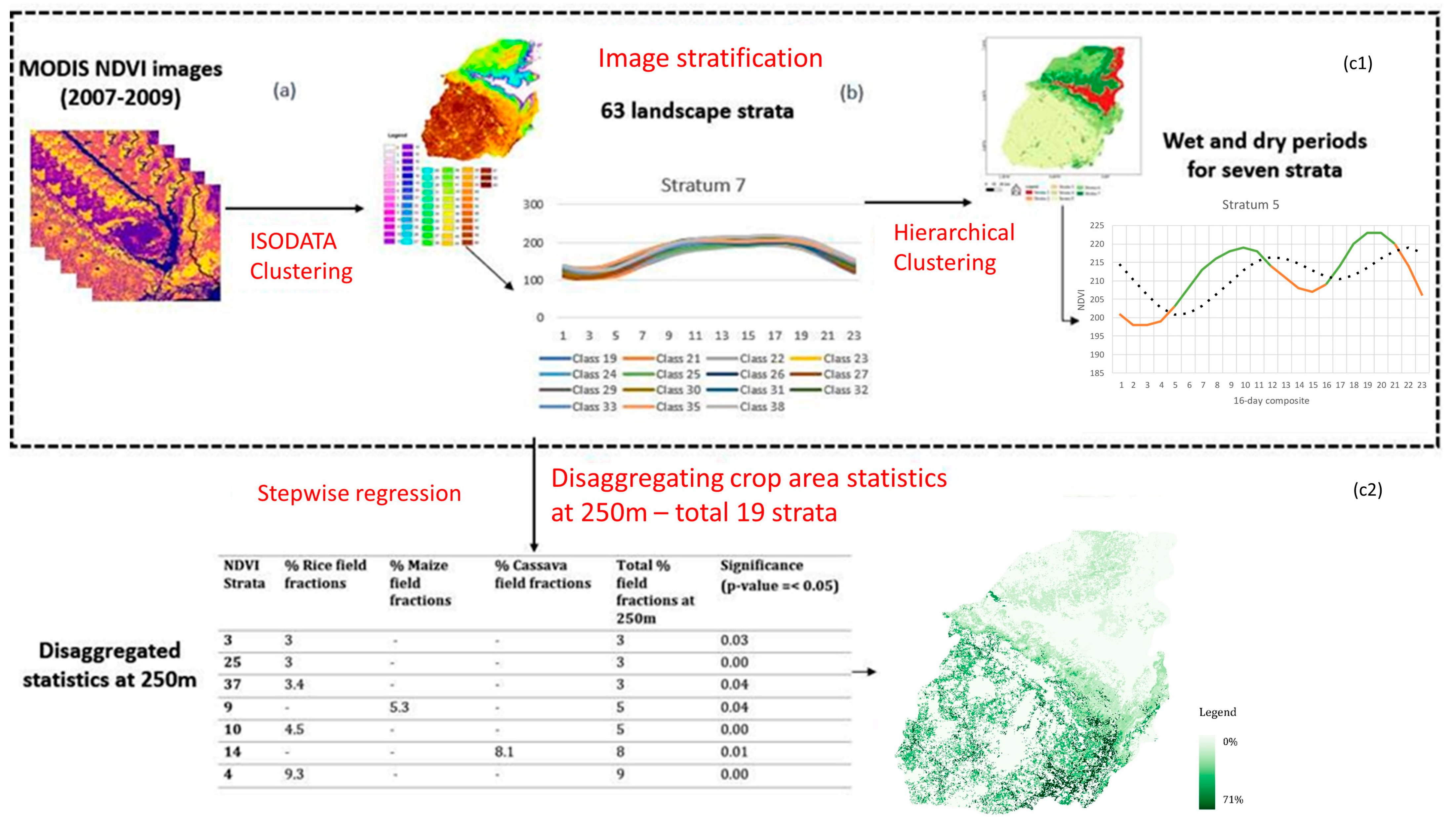
The main steps of the workflow (
Figure 2) included (i) acquiring and processing MODIS, Sentinel-1, Sentinel-2, and the SRTM-DEM images; (ii) MODIS image stratification, strata merging to derive distinct regional vegetation seasonality, and mapping 250 m arable field fractions from district-level crop statistics to landscape strata; (iii) derivation of seasonally stratified 20 m resolution spectral, polarimetric, textural, and topographic features (137 in total); and (iv) feature selection and RF classification [
27] of the arable field at 20 m resolution. This study trained the RF model with polygons digitized based on 2018–2019 PlanetScope wet and dry season near-infrared (NIR)-red-green composites within a labeling platform [
6]. The study utilized the original bands of Sentinel for deriving texture features, while vegetation indices were used for spectral features as they were found to be more important than original bands for crop mapping in sub-Saharan African countries [
14].
3.1. Acquisition and Processing of Satellite Data
Satellite images were accessed via the Google Earth Engine cloud computing environment or acquired from third-party sources. All images were resampled to 20 m resolution using the nearest neighbor technique and projected to UTM zone 30N. The strata were derived from MODIS Terra+Aqua NDVI 16-day maximum value composites from 2003 to 2009. The composites were used in a previous study by Ali [
18]. The authors used the vegetation index quality band to mask pixels containing haze, clouds, and other atmospheric noise. The remaining artifacts were filtered with an adaptive Savitzky–Golay method in TIMESAT
®.
The polarimetric, spectral, and corresponding textural metrics were derived from Sentinel-1 and Sentinel-2 from 2017 to 2019 dry and wet season median composites. Here if the area had more than one dry/wet season, all of the dry/wet seasons were combined, resulting in one composite per season (dry/wet). The location and extent of arable fields did not change substantially over the three-year (2017–2019) period of study was assumed. The three-year period was needed to ensure that cloud-free pixels were available, especially in the wet season, as approximately >50% of available Sentinel-2 scene images in GEE had more than 50% of cloud cover annually.
Sentinel-2A and B L2A images were used, with a five-day return frequency and spatial resolution of 10–20 m. Prior to April 2017, only Sentinel-2A data were used because Sentinel-2B was not yet launched. A total of four scenes and 200+ images per scene were processed. The Sentinel-2 level-1C 2017-18 images were downloaded from the USGS Earth Explorer and converted to surface reflectance using the Sen2Cor level 2A processor [
28]. 2019 L2A images were used using GEE. The accompanying scene classification band was used to mask clouds, cloud shadows, and haze.
Sentinel-1A and B C-band level-1 ground range detected (GRD) SAR was used with dual polarization (VV and VH) in the interferometric wide (IW) swath mode, and the intensity values were in dB at 10 m pixel size, with a return interval of six days for the ascending orbit. The images were pre-processed with GRD border noise removal, thermal noise removal, radiometric calibration, and terrain correction [
29].
A total of five scenes of void-filled 30 m resolution SRTM-DEM tiles overlapping the study were used from the USGS Earth Explorer to derive the topographic metrics—slope, and elevation.
Daily ortho-rectified 2018 PlanetScope Analytic surface reflectance imageries were downloaded from the Planet API [
23] and converted into two seasonal composites—growing season (May–September 2019) and dry season (December–February 2019).
3.2. Municipality-Level Crop Statistics
The Statistics Research and Information Directorate (SRID) of the Ministry of Food and Agriculture (MoFA), Ghana, provided the crop area statistics for rice, maize, and cassava from 2005 to 2009. The dataset consisted of the annual crop area for rice, maize, and cassava for 17 districts. The crop area was averaged for each crop over five years.
3.3. Image Stratification and Mapping 250 m Arable Field Fractions
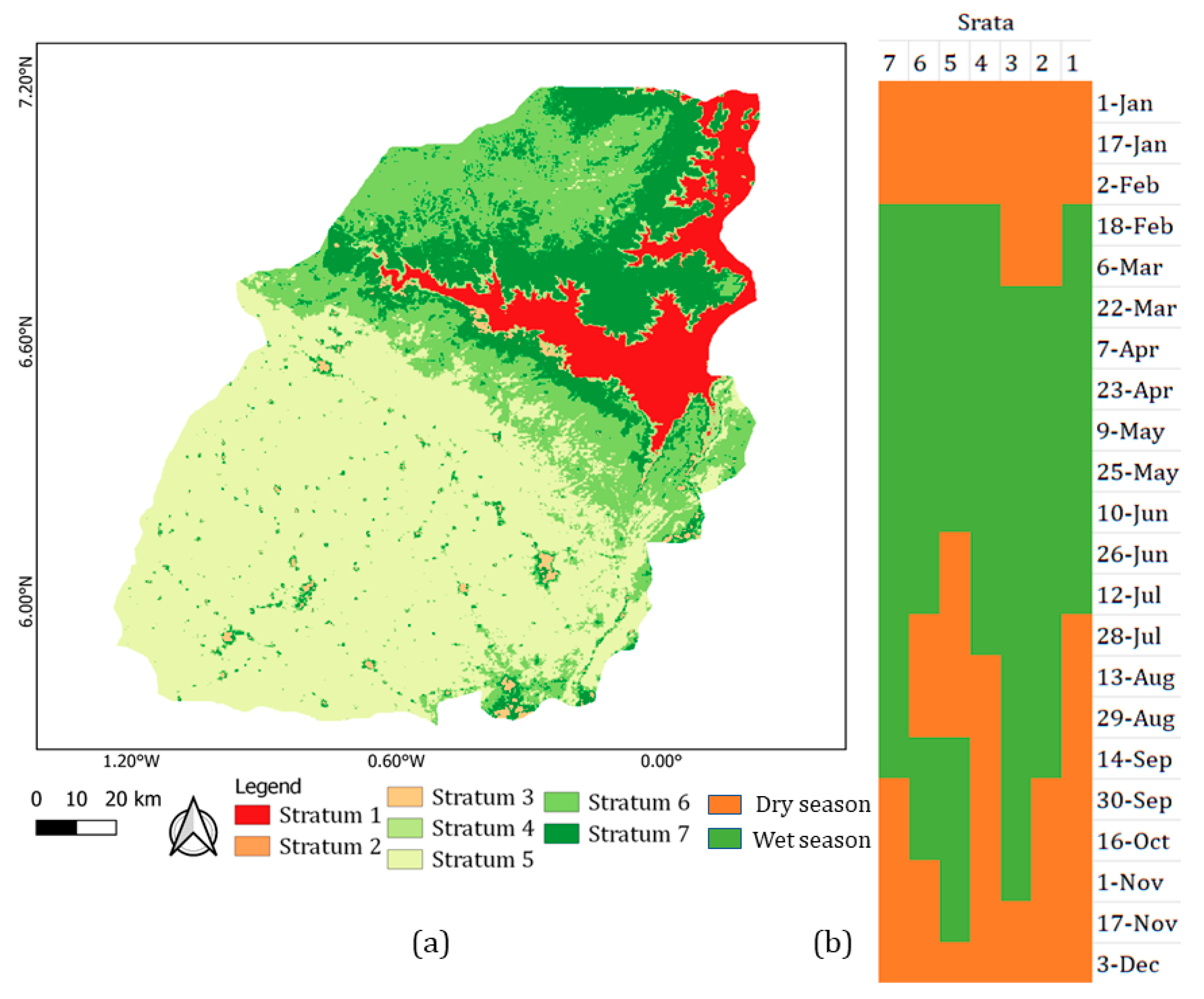
The general workflow of stratification included three steps. The first step entailed stratifying the whole region into 63 regions using ISODATA clustering. The second step was to map distinct vegetation seasonality by grouping the strata’s temporal profiles with similar seasonalities but with different amplitude (
Figure 3b) using hierarchical clustering, resulting in seven strata. The last step was to use the initial 63 landscape strata to disaggregate district-level crop statistics using stepwise regression, giving 19 strata of a potential arable area at 250 m.
The ISODATA clustering algorithm classified the MODIS NDVI 16-day composites into landscape strata. ISODATA is an unsupervised classification technique. It iteratively combines, splits, and removes classes to minimize within-class and maximize between-class pixel variability [
30]. The default set parameters in ENVI version 5.3 (Exelis Visual Information Solutions, Boulder, CO, USA) were used for clustering: a 2% threshold and ten iterations. It generated 63 strata. However, many of the strata exhibited similar temporal profiles with a difference in magnitude of NDVI values, so these strata were combined into seven unique strata using hierarchical clustering [
31]. Hierarchical clustering computes the Euclidean distance between each observation and puts it in its cluster; in this way, it combines similar clusters and separates the different groups of clusters by giving the hierarchical order for all the cluster input.
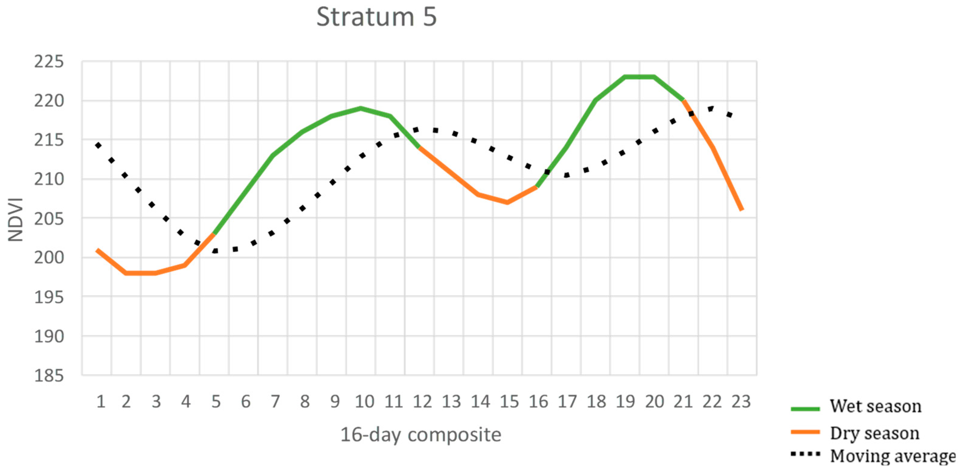
The wet and dry periods were defined with the delayed moving average method [
32]. The method uses a moving average of the NDVI temporal profile to signal the start and end of wet periods. A wet period begins when the ascending arm of the NDVI profile crosses the moving average NDVI profile and ends when the descending arm crosses (
Figure 4). Periods outside the wet periods are considered dry. The method accounts for multiple modalities of rainfall, but these were not separated into major and minor seasons since it changes from stratum to stratum. A 3 month moving average was selected to approximate the length of the primary growing season.
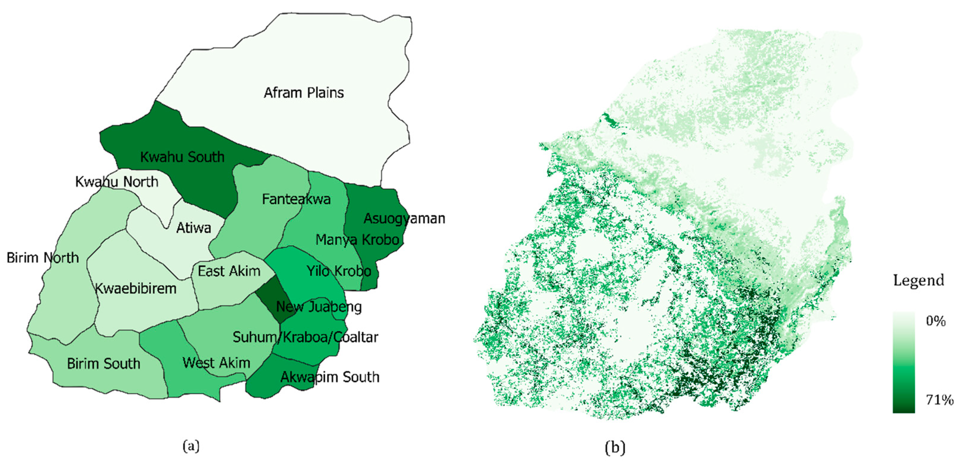
The crop area statistics were disaggregated per stratum using multiple stepwise linear regression at 250 m resolution, according to de Bie [
20]. The model can be expressed as:
where Y is the district-wise crop area, β
1, β
2, …, β
n are beta coefficients, and C
1, C
2, C
3, …, C
n is the area of a specific stratum for a particular district.
Only area statistics for the main staple crops in the region (maize, cassava, rice) were considered. Stepwise regression is a multivariate linear technique that iteratively selects features with statistically significant partial correlations with model residuals. Here, it was done by adding features to the model one by one (forward mode). Then, the fitted coefficients for each stratum were summed per crop category and assigned to the respective pixels at 250 m resolution.
Strata with negative coefficients (i.e., negative area) or insignificant coefficients at 95% confidence were assigned zero field fractions. These resulted in 19 strata with significant coefficients. These 19 strata were expressed as % of total arable field fractions at 250 × 250 m pixel size as a categorical variable in the model as it merely captures the higher spatial variations of arable fields in the landscape.
3.4. Derivation of Spectral, Polarimetric, Textural, and Topographic Features
A total of 14 dry and wet season spectral vegetation indices derived from Sentinel-2 were evaluated (
Table 1). These included NDVI and Normalized Difference Water Index (NDWI), the ratio of NIR and SWIR, which measures the vegetation water content. Others included the brightness index, Chlorophyll red-edge (Chlre) index, and narrow band red-edge Normalized difference vegetation indices (NDVIRE1, NDVIRE2, NDVIRE3). The brightness index indicates soil brightness [
33], which is sensitive to soil color, humidity, and salinity. The Chlre distinguishes chlorophyll pigments (a + b) and reduces the impact of intra-species reflectance variation better than other spectral regions [
34]. Similarly, the narrowband red-edge NDVIs are more sensitive to plant chlorophyll content than broadband indices [
35].
Ten dry and wet season polarimetric metrics were derived from the Sentinel-1 radar backscatter coefficient (
Table 1). These included VV, VH, cross-ratio (VV/VH), and arithmetic intensity parameters (VV − VH and VV + VH). The values of SAR backscatter in VV and VH can be affected by canopy structure (vertical and horizontal), vegetation water content (due to distinct dielectric constant of ground targets), or underlying surface roughness [
36,
37,
38]. The cross-ratio (VV/VH) at specific incidence angles was found to be more sensitive to crop growth stages, specifically near tillage, than the individual backscatter [
39,
40]. Both VV and VH images had very bright pixels (i.e., high backscatter coefficient values) on the edges of mountains likely because of geometric distortions such as layover and foreshortening. In GEE, these geometrically distorted pixels were masked by generating a mask from Kakooei [
41]. This mask was calculated using slope, aspect, Sentinel-1 orbit, and incidence angle. No additional speckle filtering was applied because the images were down-sampled to 20 m by spatial averaging.
Five grey-level co-occurrence matrices (GLCMs) textural metrics proposed by Haralick [
42] were included to account for the spatial dependencies in croplands and other land cover types. GLCM is a second-order statistical method that calculates the number of occurrences of specific paired pixels at a given distance and angle. The statistics were homogeneity (measures frequency of uniform occurrences), dissimilarity (counts different combinations present in the window), contrast (measures the levels of grey-scale local variation), GLCMvariance (measures the local dispersion around the mean), and entropy (measures disorder or spatial arrangement). The statistics were derived for Sentinel-1 polarizations and Sentinel-2 spectral bands. The parameter of window size was set to 11 × 11 for the four cardinal directions, with default parameters as one angular distance and a probabilistic quantizer based on previous studies in heterogeneous and fragmented landscapes [
43]. The textural analysis yielded a total of 110 features.
Table 1.
Image features included in the model.
Table 1.
Image features included in the model.
| Category | Image Features/Equation | Reference |
|---|
Spectral features
(total 14;
7 for dry and 7 for wet season) | NDVI = (B8 − B4)/(B8 + B4) | [44] |
| NDVIRE1 = (B8A − B5)/(B8A + B5) | [35] |
| NDVIRE1 = (B8A − B6)/(B8A + B6) | [35] |
| NDVIRE1 = (B8A − B7)/(B8A + B7) | [35] |
| Chlre = (B7/B5) − 1 | [34] |
| NDWI = (B8 − B12)/(B8 + B12) | [45] |
| Brightness = sqrt((B4 × B4)/(B3 × B3)/2) | [33] |
Polarimetric features
(total 10;
5 for dry and 5 for wet season) | VV | - |
| VH |
| VV − VH |
| VV + VH |
| VV/VH |
GLCM texture features
(total 110;
5 × 2 (S1 bands—VV and VH) and 5 × 9 (S2 bands) for dry season;
similarly, for the wet season) | Homogeneity | [42] |
| Dissimilarity |
| Contrast |
| GLCMvariance |
| Entropy |
Topographic features
(total 2) | Slope | - |
| Elevation |
MODIS long-term disaggregated statistics
(Only 1) | - | [20] |
We also used two topographic metrics as model predictors, including the elevation and the percent slope, which were calculated using the ee.Terrain GEE package [
29].
3.5. Model Training and Testing Data
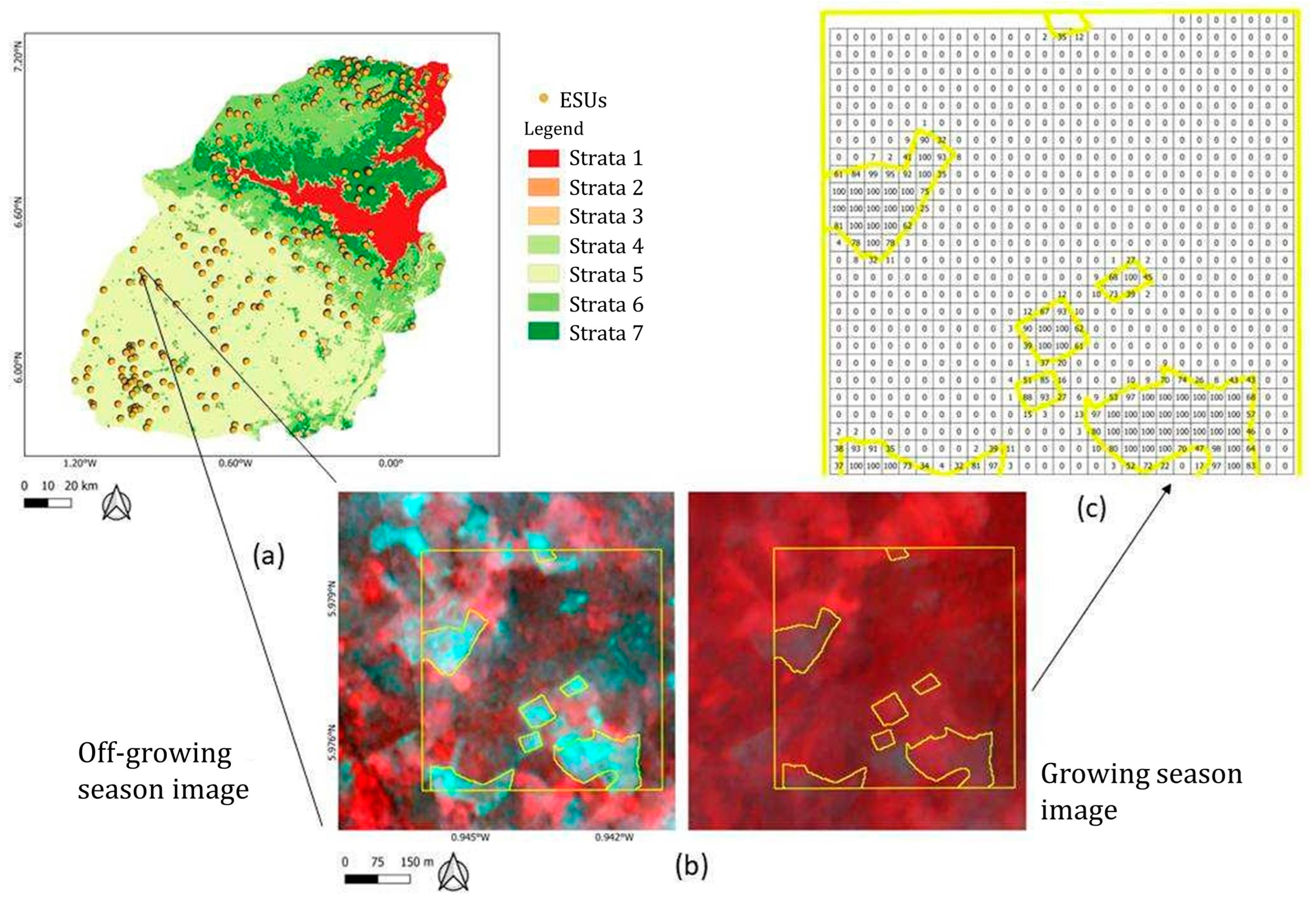
A total of 600 elementary sampling units (ESU) of size ~550 × 550 m were digitized over the study area using labeler (
Figure 5a), which provides a convenient interface for digitizing croplands and other land cover types using PlanetScope imagery over large areas. Labeller was used during a previous study [
6] to develop training/testing samples over 16 areas of interest (AOIs) across Ghana. Out of which, four of the AOIs fall within the Eastern region. The ESUs were randomly selected in each of the AOIs. In this study, additional ESUs were added for two of the seven seasonal strata because they were under-sampled.
Arable fields were visually identified using available pairs of dry (December–February 2019) and wet season (May–September 2019) PlanetScope images (
Figure 5b). The resulting polygons were then extracted from the labeler’s database and superimposed over a Sentinel-2 20 m pixel grid to calculate arable field fractions (
Figure 5c). This intersection between the 20 m grid and labels resulted in a total of 625 samples with values ranging from 0 to 1 per ESU. The procedure yielded 336,555 samples to train the RF model. The samples in the labeler platform were crowd-sourced; thus, as quality control to avoid low-quality samples in modeling, the dummy RFclassifier was trained on the whole dataset, and areas with higher uncertainty were flagged. The uncertainty of samples was measured as the difference in actual occurrence versus the probability produced by a vote-counting method. The uncertain flagged areas were re-digitized only if needed using visual observation. Pixels falling across field boundaries (0 < pixel value < 1) were omitted to prevent mixed pixel effects. Finally, a total of 282,114 samples remained after these filtering steps for the final model building.
3.6. Variable Selection and RF Classification
The remote sensing community widely uses RF for land cover classification because it is less prone to over-fitting and yields models with more predictive power and lower error than other methods [
46]. Like other machine learning methods, however, RF is susceptible to over-fitting when irrelevant or redundant features are included in the model [
47]. Therefore, Recursive Feature Elimination (RFE) was implemented in this study to remove irrelevant or redundant features [
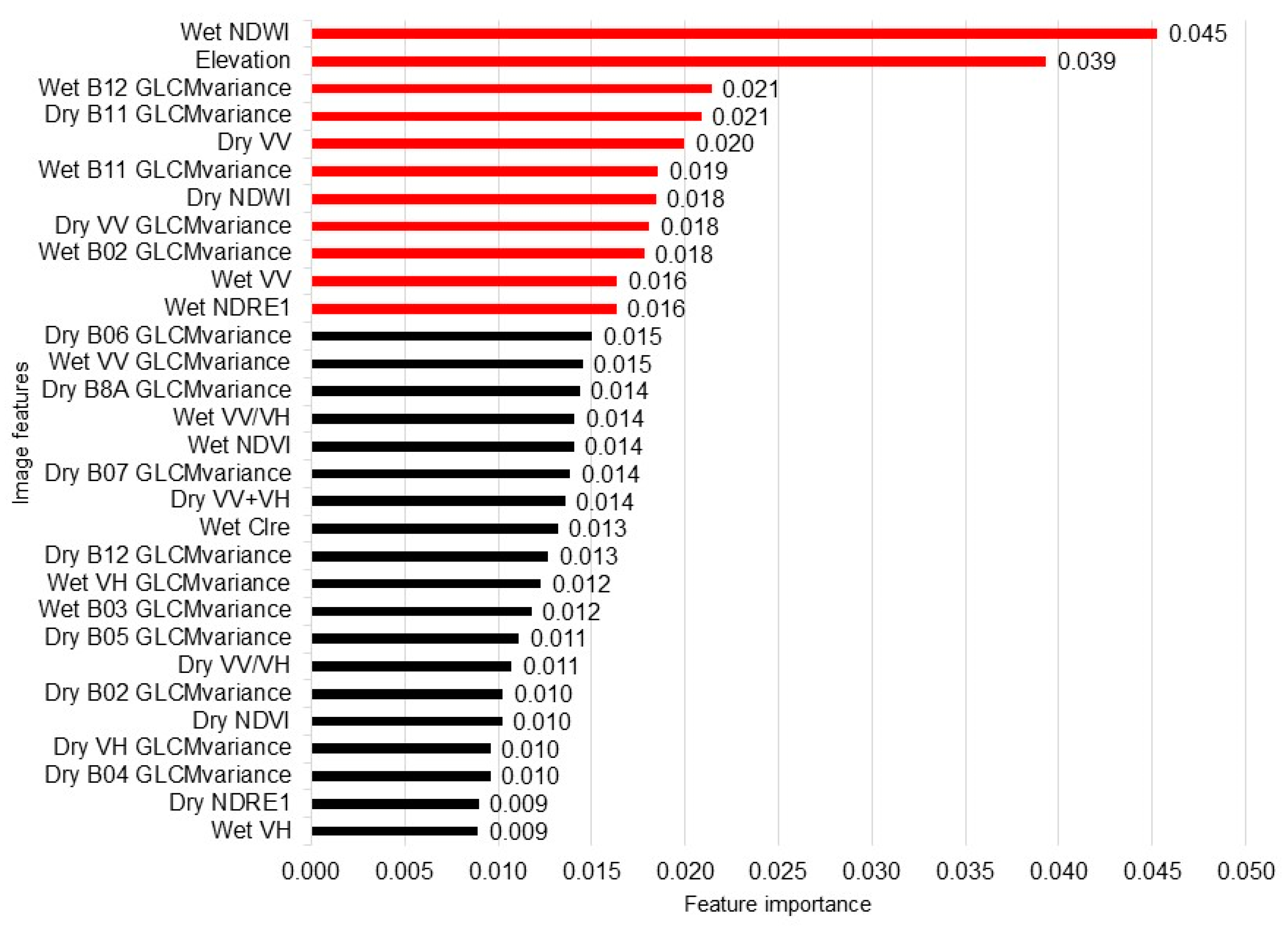
48]. RFE is a wrapper function that iteratively removes features from the model that do not contribute to the predictive power of the model. In this study, 10-fold cross-validation (CV) was used for RFE. The model’s predictive power was assessed with the receiver operating characteristics area under the curve (ROC-AUC, Area Under the Receiver Operating Characteristic) at each fold for a specific set of features. The increase in the model’s ROC-AUC score by adding features one by one was reported. The features contributing ≥0.05 to AUC were selected for final predictions. The final feature importance was reported as an importance score calculated by averaging Gini importance scores across each fold produced by RFE.
The sample set was split 70–30% for model training and testing. The RF model consisted of 500 trees developed over 100 iterations and a 10-fold CV. The class weights were chosen ‘balanced’ while bootstrapping RF as higher observations were present for the non-arable area than the arable area. The ‘balanced’ class weight option available in sci-kit-learn (package in Python) assigns automatic weight to the classes, which is inversely proportional to the number of samples. The model performance was assessed using AUC, accuracy, balanced accuracy, precision, recall, and F1-score. Balanced accuracy is the weighted average version of accuracy, which considers the number of observations of each class in the dataset. Precision shows the total relevance or confidence in the prediction and recall explains the correct class prediction out of all specific class samples or completeness of the predictions. The F1-score is a composite measure of precision and recall.
Unlike the regression models, in the classification model, the continuous functional relation between image features and predictions is often not established because the predictions in classification models are categorical. However, RF makes predictions of a specific class using multiple predictions made by individual estimators (trees) using the vote-counting method. The number of votes or probability of an observation being within a particular class, is continuous. In addition to the advantages of easy interpretability, feature importance, and computational efficiency compared to other machine and deep learning models, RF also offers the ability to analyze the relationship between features and predictions through Partial Dependence Plots (PDPs). PDPs in machine learning use specific class probabilities and one or specific set of features while marginalizing the other features, to explain the linear or non-linear relationship between features and model predictions [
49,
50]. As opposed to sole dependence on feature importance, here, the image features and their detailed relation to arable field distribution were explained via PDPs. In this study, PDPs explained the changes in the probability of occurrence of arable fields with changes in image value.
5. Discussion
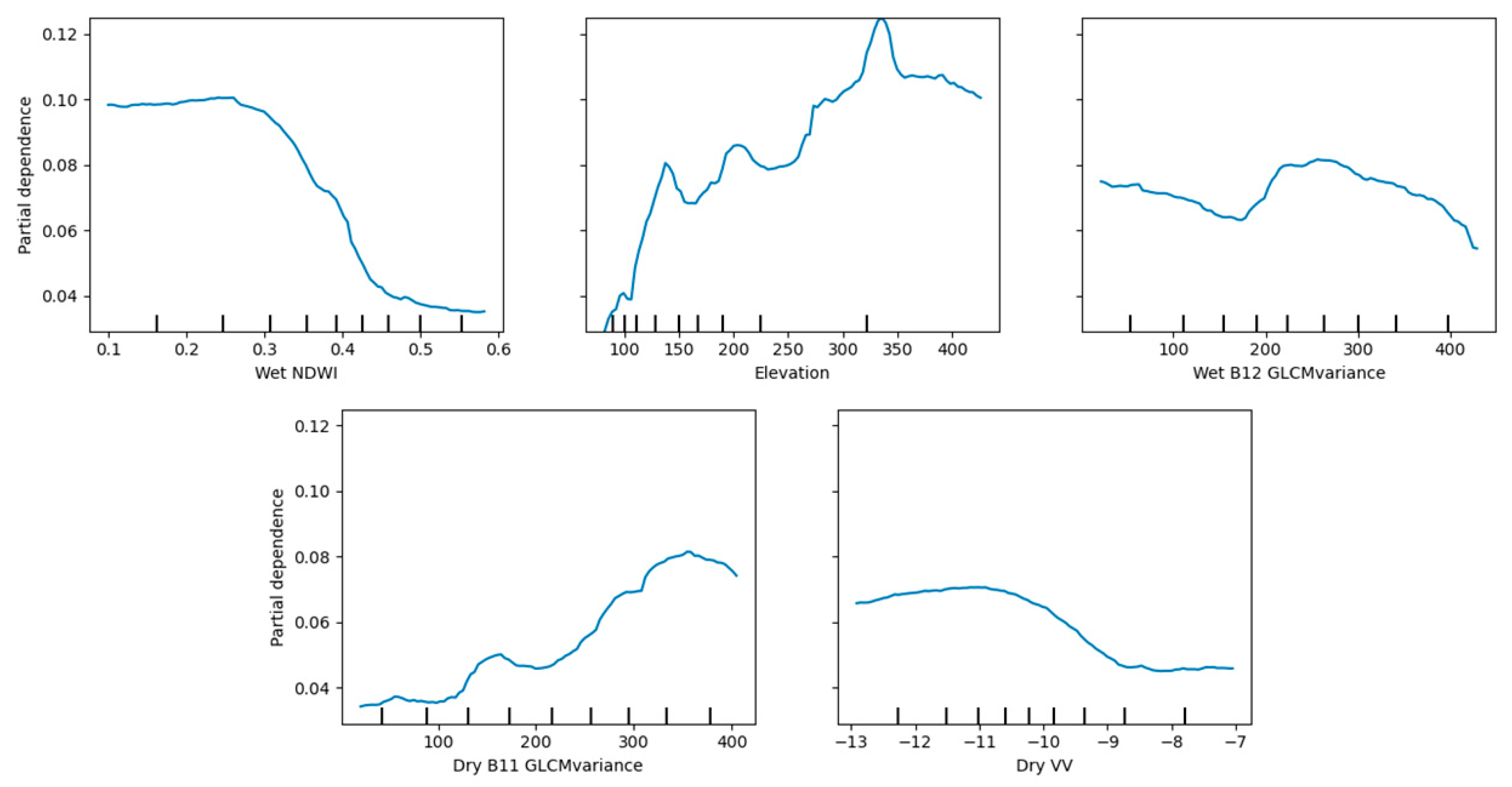
This study concluded three major findings; (i) Sentinel-2 image features, especially SWIR features, explain the most variation in arable field area followed by Sentinel-1 polarimetric (VV) and topographic features (elevation); (ii) Sentinel-1 and Sentinel-2 texture features at moderate spatial resolution (20 m) are important for arable area mapping; and (iii) diversity in crop calendars in fragmented agricultural landscapes can be accounted using the simple technique of image stratification to derive seasonally stratified higher spatial resolution image features. The dry season predictors were as important as the wet season in the regular (annual) mapping of the arable area.
A previous study [
14] found that Sentinel-2 SWIR-based indices, sensitive to soil and vegetation moisture status, are better at discerning croplands with relatively high moisture variability from natural vegetation and built-up land cover in dry climates region. Approximately a third of our study area was also dry, which is why NDWI and SWIR texture bands were the most important. Orbiting (PRISMA, ENMAP) and upcoming (ESA CHIME, NASA SBG) hyperspectral missions include dozens of narrow bands in the SWIR. These missions should be exploited to improve cropland mapping in dry areas. Sentinel-2 features were found to be more important than S1 features. This could be because of the sensitivity of radar backscatter intensities to surface roughness, canopy structure, and moisture content proposing inverse ill problem and making the predictor less sensitive to the arable field area. In order to address this limitation in future studies, it is recommended to incorporate a dual-pol radar vegetation index (DpRVI). The DpRVI utilizes both the degree of polarization and backscatter intensities, which could offer increased sensitivity to crop growth [
51]. Husak [
5] and Mohammed [
21] showed the highest probabilities of arable fields increased at intermediate elevations and plateauing around 2500 m. This study also showed an increase in arable fields with elevation but below 325 m. In the study, elevation broadly captures the climatic regions of the study area, making it an important predictor for the arable area; however, relatively flat terrains can be found in countries such as Zambia with overall elevation <1000 m; in such cases, slope could be more useful. In the study, most cultivated areas were on hills, making a slope a less important predictor than elevation. Please note that in this study, the significance of individual sensor datasets was determined by combining the feature importance scores of selected features for each sensor, rather than through an ablation study. Because the primary objective of the study was to analyze the complementary effects of different sensor datasets for cropland mapping. Although the study did not include an ablation study, it is anticipated that similar results would be obtained if one were conducted. The study concluded that texture features were the most crucial (half of the total 11 features), followed by spectral and polarimetric features. This suggests that the spatial arrangement of pixels is more significant than the value of the pixel intensity. These arrangements can be expressed through measures of contrast (differences) or homogeneity (similarities) with neighboring pixels, or through degrees of randomness or variability such as entropy or variance. Out of these options, only GLCM variance texture features were deemed important, indicating that the total variation in pixel intensity (i.e., the arrangement of pixels) is more important than the relative pixel intensity. For instance, urban areas showed a higher degree of variation due to their random and complex arrangement of pixel intensity compared to forested areas with lower degrees of variation (see
Figure 11). Nevertheless, the significance of texture features may require verification in temperate climates, where larger agricultural holdings, organized field patterns, and climate-specific cultivation practices are prevalent. Landscape stratification and re-merging strata with similar seasonality (seasonal strata) using long-term average MODIS NDVI phenology, a method employed in this study, is the simple, easy, and accessible method to capture the crop calendar diversity. The study area in the region exhibited differences in growing season partially because of rainfall patterns, whereas the rain-fed region in the south had two distinct dry and growing seasons. In contrast, the north region had one prolonged growing season and only one dry season due to the availability of irrigation facilities. This suggests that long-term NDVI strata-based vegetation seasonality could be better than following rainfall patterns to derive dry and wet seasons. The landscape stratification proved valuable in discriminating crop seasonalities but not in disaggregating crop statistics for model-building. This is somewhat contradictory to Mohammed [
21], who found disaggregated statistics to be the most important predictor of arable field fractions at 30 m spatial resolution. Mohammed [
21] used 1 km PROBA-V NDVI whereas this study used 250 m MODIS NDVI. Stratification, which is a generalization of climate and other factors impacting farming practices, may be more effective at coarser spatial resolution data. Here the model also included several finer spectral and textural features, which proved to be more important than lower spatial resolution features. Lastly, Mohammed [
21] considered the field fractions as different features according to strata that, when taken together, explained the most variance in arable field fractions. Our study considered the 250 m field fractions as a single feature. This study establishes that MODIS NDVI climatology effectively captures farming patterns and facilitates the stratification of finer spatial resolution features. However, it should be noted that this generalization may not apply as easily to temperate regions, which typically exhibit more pronounced seasonal variations with distinct growing and dormant periods. Whereas in sub-Saharan regions, pixel-wise seasonal stratification becomes necessary to accurately capture the agricultural dynamics. Further exploration is required to compare the importance of pixel-wise seasonal stratification in different climates and agricultural landscapes.
The utilization of PDPs can facilitate the comprehension of the intricate relationships between image features and model predictions in machine learning models. This approach can broaden our comprehension of model predictions and provide insights into how changes in image values affect them, thereby adding more meaning to remotely sensed images. For example, NDWI increases as water thickness in canopies increases. It ranges from 0 to 1 but seldom exceeds 0.40. Here, the threshold reported in PDPs was 0.35 during the wet season, separating dry and well-watered arable fields from extremely moist natural vegetation. Natural vegetation tends to maintain high moisture levels throughout the year because it has more extensive root systems and greater access to water stores. PDPs also showed that SWIR GLCMvariance increased during the dry season and decreased during the wet season for arable fields, while wet areas such as forests and water maintained low GLCMvariance (<100) and complex urban areas maintained higher variance (>380) throughout the year. Arable field occurrences were higher in a narrow range (200–300) of variance for the wet season compared to the dry season. This could be because of the sensitivity of SWIR towards vegetation water content in the wet season. Sentinel-1 VV intensities, on the other hand, distinguish the vegetation biomass. The transition in dry season VV at −9 to −10 could be associated with a higher biomass of shrubs and tall canopies compared to bare soil of arable fields, while higher values (≥−7) are related to complex urban structures.
Machine learning requires many samples for model building, which were incorporated by including >300,000 samples collected. An inaccurate or imbalanced sample set affects machine learning performance adversely [
23], especially crowd-sourced samples are prone to such errors or imbalances of samples. This study maps uncertainty in samples using dummyRF predictions to avoid extreme errors; however, the quality of the labels can further be improved using the advanced techniques provided by the labeler platform, such as creating consensus labels across multiple labelers [
6]. Usually, for cropland mapping, non-occurrence is much more frequent than occurrence, causing an imbalanced sample set. This study assigned automatic class weights where less frequent arable areas had higher weights to incorporate imbalance in the dataset. Although, there could still be a large impact of an imbalanced sample set in model predictions because the model’s accuracy was 97% whereas the balanced accuracy, AUC was 0.78, and F1-score was 0.85, showing that accuracy tends to inflate when the sample set is imbalanced. Future work should incorporate un-supervised clustering of non-occurrence samples only and select samples proportionally to the number of observations in each cluster to preserve information for other classes (natural vegetation, forest, urban, water bodies) while creating the balance sample set. Either generating synthetic occurrences or optimally removing non-occurrence samples in the future can improve the assessment of model performance and model transferability [
52].
The study highlights the importance of methodological improvements by creating better temporal, spectral, and contextual information for arable area mapping. Low spatial high temporal MODIS NDVI data can effectively map distinct vegetation seasonality and can be utilized to stratify finer Sentinel features. Sentinel-2 SWIR features, followed by Sentinel-1 co-polarized (VV) features and elevation data can improve arable area mapping accuracy. Incorporating texture features that exhibit spatial arrangements of pixels is essential for arable mapping in the sub-Saharan region.
6. Conclusions
Effective and reliable cropland mapping in the tropics remains challenging because farming practices vary considerably, fields tend to be small and irregularly shaped, persistent cloud cover throughout much of the growing season, and poor quantity/quality of training data. The study evaluated image stratification and Sentinel-1 and -2 data integration to overcome these obstacles to cropland mapping in Ghana.
This study makes three important observations. First, Sentinel-2 SWIR (moisture-related) and Sentinel-1 VV (biomass-related) metrics were the most effective at separating croplands from natural vegetation or built-up land cover. Sentinel-2 greenness-related indices (red-edge, NIR) were less important, probably because of the large differences in moisture availability in the study area. The elevation is essential to model building, as it largely defines what crops are grown where. However, the elevation relationship must be considered on a landscape basis, given differences in climate, soil, and other constraints on farming. Second, nearly half of the most important features were texture-based. Texture accounts for spatial differences in land cover types, considering the small size, irregular shape, and transient nature of fields in the study area. Third, image stratification is an easy and accurate way to capture considerable differences in farming practices.
To enhance the model’s performance and transferability, future research should focus on optimizing sampling strategies that balance the arable and non-arable areas. Specifically, non-arable samples should be filtered out to represent other land cover classes accurately. Additionally, to better differentiate arable areas, the use of a new hyperspectral mission with more SWIR bands is recommended, as this will enable the capture of narrowband pixel intensity on a larger scale using space-borne images. Furthermore, the exploration of full polarization radar images or advanced radar vegetation indices to capture precise crop biophysical growth should be further investigated.
