Utö Observatory for Analysing Atmospheric Ducting Events over Baltic Coastal and Marine Waters

Abstract

Maritime safety relies on navigation, detection, and radio communication technologies that function through electromagnetic radiation. Propagation of electromagnetic radiation can be impacted by a disruptive phenomenon known as ducting. Our four-week study using a X-band coastal radar and various meteorological and marine observations, including vertical profiles of temperature, humidity and wind, in early spring 2022 concluded that the combination of measurements at the Utö observatory provides a reliable means of detecting ducting in the Archipelago Sea. The modified refractivity calculated from the vertical profiles for the 22–59 m and 32–59 m altitude layers and coastal radar over-the-horizon observations agree 77% and 85% of the time, respectively. As such, the modified refractivity gradient can be considered a good indicator for over-the-horizon detection with the Utö coastal radar over the open sea. The horizontal wind profiles also revealed a low-level jet at the radar height that often coincided with the ducting observations. To quantify the results, we created an empirical ducting index which showed that ducting is spatially variable, showing the capabilities of the Utö observatory for research oriented towards monitoring and improving maritime safety and security.

1. Introduction

Marine traffic and security depend on navigation, detection, and radio communication technologies that function through electromagnetic radiation, which can be impacted by the disruptive phenomenon known as ducting. Ducting is a form of anomalous signal propagation where, due to factors that can include temperature inversion and strong negative vertical humidity gradients, electromagnetic radiation becomes strongly bent (refracted) towards the Earth’s surface and becomes trapped in a horizontal layer above the surface, a duct. Whether or not the signal is within or outside the duct affects how far the signal can travel, and therefore influences the radar range. The radar horizon typically extends up to tens of kilometres under standard atmospheric conditions but can be extended to hundreds of kilometres in conditions favouring ducting. As observations of fixed targets beyond the standard radar horizon can be attributed to ducting, the coastal surveillance extended horizon can be used to study the frequency and strength of ducting.

Ducts can be divided into two categories based on their height: surface, and elevated ducts. Surface ducts are further divided into standard surface ducts and surface-based ducts. Besides their height, ducts can be separated into classes based on the governing formation processes. These include evaporation, advection, subsidence and radiative cooling ducts [1]. The most commonly studied class is evaporation ducts, used to describe humidity-driven ducts where the refractivity gradient decreases rapidly without requiring a coinciding temperature inversion. As such, evaporation ducts are found over large bodies of water. Evaporation ducts are the most commonly occurring duct type and are often considered a near-permanent global phenomenon. Hence, extensive focus has been on studying the influence of evaporation ducts on radar and radio communications [2,3,4,5,6,7].

The effect of evaporation ducts on coastal radars depends on how the duct height and thickness relate to the height and grazing angle of the radar [6]. The effect of duct thickness also depends on radar frequency [8]. If the coastal radar signal becomes trapped in the evaporation duct, detection over the standard horizon can occur [6]. However, if the radar signal is not trapped, objects within the evaporation duct can be left undetected even within the standard horizon [6]. Moreover, evaporation ducts are also associated with a reduced radar signal strength and shorter range of detection [4]. Even though evaporation ducts are the most common duct type, surface-based ducts have been found to be stronger and have a larger effect on the radar range [9]. In a recent study by Huang et al. [9] vertical profiles of refractivity measured with instruments mounted on a mast on a platform above the sea and a coastal 9400 MHz navigation radar were used to study the relationship between detection over the standard horizon, referred to as over-the-horizon detection hereafter, and evaporation ducts. They found that evaporation ducts only enabled weak over-the-horizon detection while long-range over-the-horizon detection was found to coincide with the presence of a lower atmospheric duct. However, the significance of evaporation ducts cannot be overlooked due to their effect on radar detection capability near the surface, with recent studies investigating the influence of ducts on X-band over-the-horizon detection using duct modelling [10,11,12].

Measuring duct characteristics, such as frequency, height, depth and intensity, requires vertical profiles of refractivity. Vertical profiles of refractivity can be achieved indirectly by measuring vertical profiles of humidity, temperature and pressure, traditionally achieved using a radiosonde [13,14,15,16]. Radiosonde measurements are routinely taken globally and have fine vertical resolution but are expensive and therefore the measurement frequency is coarse. Measurements taken with instruments mounted on a mast have also been previously used, both on land and aboard research vessels [9,10,17,18,19]. Mast measurements can provide continuous vertical profiles of the lower troposphere, the vertical resolution of which can be tailored to the measurement environment and purpose. In a marine environment, the interest is near the sea surface due to the presence evaporation ducts but mast measurements within a few metres of the sea’s surface are often limited by waves, storm events and corrosive sea spray.

In this study, we use a variety of meteorological and marine observations, including vertical profiles of temperature, relative humidity and horizontal wind, alongside an X-band coastal radar, to assess whether the marine radar research facility developed at Utö provides the means to observe and analyse ducting over coastal and marine waters of the Baltic Sea. The study uses measurements from a four-week period in early spring 2022 when prominent ducting was observed during the second half of the study period. An empirical ducting index was created to identify and quantify ducting events from the coastal radar data. The index can be applied to the whole radar network alongside the mast measurements, and be used in validating numerical weather model-based ducting forecasts.

2. The Utö Observatory

The Archipelago Sea (between 59.7$°$N and 60.6$°$N, and 20$°$E and 23$°$E) in the Baltic Sea covers an area of 8300 km${}^2$, with thousands of small islands and islets (Figure 1). The mean depth of the sea is only 19 m, although the deepest points can exceed 100 m. The geometry of the Archipelago Sea is complex, and based on regional characteristics, it can be divided into the outer, middle and inner archipelago [20].

Annual average temperatures in Utö, an island located in the outer Archipelago Sea, are around 6.7 $°$C with the lowest wintertime temperatures below $-20{}^{°}$C and the highest summer temperatures above 25 $°$C. The sea ice cover in the area is highly variable; shallow protected areas are ice-covered almost every winter while outer areas may remain without ice. The average duration of the ice-covered season around Utö during the period 1981–2020 was 27.8 days, starting in January or February and ending in March or April [21]. Sea ice concentration and thickness charts for the Baltic Sea used in this study are available via the Copernicus Monitoring Environment Marine Service (CMEMS) database [22,23]. The monthly average sea surface salinity at Utö varies between 6.3 and 6.7 $\mathrm{g}{\mathrm{kg}}^{-1}$, with the lowest salinities observed during the summer, and the sea surface temperature (SST) long-term averages ranging from zero during the winter to 16 $°$C during the summer. For short periods during summertime heat waves, SST can reach values as high as 25 $°$C.

The Utö radar research facility is part of the Utö Atmospheric and Marine Research Station [21]. The Utö coastal radar is an X-band radar produced by Navielekro ky and mounted on a pilot station tower at Utö. The radar is equipped with a radar data recorder that digitises the analogue radar control signals and radar video with 20 MHz. The software rasterizes the radar echoes into a plan position indicator (PPI) image per radar revolution [24]. For the ducting research purposes the radar pulse repetition frequency has been reduced to 1 kHz corresponding to a maximum unambiguous range (or observation distance) of 150 km.

Ducting is studied from 150 × 150 km square images in which the radar range appears as a circular area with a 150 km radius. The rasterization includes interpolation of radar echoes to pixels that are not intersected by the radar beam lines. However, it is also possible to study raw data consisting of radar echoes and their distances and directions. As the digitising and rasterizing of the analogue data includes both analogue adjustments of the signal level and post-processing of the image for good visual appearance, the pixel intensity values do not have a direct physical equivalent. However, as the digitisation and rasterization settings have been kept unchanged during the period of this study, the relative intensities can be reliably used to study the effects of ducting on the visibility of distant targets.

Properties of the radar are given in

Table 1. Properties of the Utö coastal radar.

Parameter	Parameter Value
Frequency	X-band (9170–9490 MHz)
Peak power	25 kW
Antenna height	34 m agl
Beamwidth (azimuth)	0.38 deg
Beamwidth (elevation)	20 deg
Polarisation mode	Horizontal

. The observations directly supporting the radar research are shown in

Table 2. Observations related to radar research at the Utö observatory. Heights given are relative to the mean sea level. Location refers to the maps in Figure 1 and Figure 2. The list of instruments is based on the situation in spring 2023, the measurement heights available during spring 2022 are indicated in bold.

Instrument	Variable	Height (m) asl	Manufacturer and Model	Location
X-band radar	radar backscattering power	48	Navielektro Ky	4
C-band weather radar	radar backscattering power	61	Vaisala WRM200	ax
Doppler Lidar	Wind profile	16…12,000	Halo Photonics Stream Line Doppler lidar	5
Acoustic anemometer	Wind, 2D	10, 32	Vaisala WMT700	2, 5
Acoustic anemometer	Wind, 3D	12, 64	METEK uSonic-3 Scientific	1, 3
T-RH sensor	Air T and RH	4, 7, 12, 22, 32	Rotronik HC2A-S3 and Vaisala HMP155EC	2
T-RH sensor	Air T and RH	59	Vaisala HMP155EC	3
ADCP	Wave spectra and sea water T	0, −23	Teledyne Sentinel workhorse 300	6
Buoy	Wave spectra, SST	0	Obscape wave measurement buoy	dx
Buoy	Wave spectra, SST	0	Datawell DWR4 Waverider	cx
AIS-receiver	AIS signal	7, 32, 55	Kongsberg RX610	2, 3
Distributed Temperature Sensing	Sea water and air T	−5…32	Silixa Ultima DTS	1, 2

and Figure 2. Other measurements at Utö are listed briefly in Appendix A.

A Halo Photonics Streamline Doppler lidar [25] is operated at the Utö atmospheric research site (5 in Figure 2) as part of the Finnish ground-based remote sensing network [26]. The Halo Doppler lidar is located on top of a container 8 m above sea level (asl). The range resolution of the lidar is 30 m and raw data is filtered with a signal-to-noise ratio threshold of 0.005 after post-processing according to Vakkari et al. [27]. The Halo Doppler lidar was upgraded to a Streamline XR version laser and amplifier in 2017.

The Halo Doppler lidar is capable of full hemispheric scanning and configured with two velocity azimuth display (VAD) scans at 4$°$ and 15$°$ elevation from horizontal every 15 min. The 15$°$ VAD scan was configured with 24 azimuthal angles and the 4$°$ VAD scan was configured with 72 azimuthal angles. Both scans were operated at 2 s integration time per ray. The VAD scans were used to retrieve vertical profiles of horizontal wind speed and direction following Browning and Wexler [28]. Excluding the three first range gates, horizontal winds can be retrieved starting from approx. 8 m above the instrument, i.e., 16 m asl. The scan sequence also includes a horizontal sector scan which is not utilised in this study. Between these scans, the lidar was operated in vertically pointing mode, configured with a 3 s integration time per profile.

3. Theory and Methods

3.1. Refractivity

Radar and electromagnetic signal propagation in the atmosphere is impacted mainly by the properties of the media [29]. The main properties that influence the signal propagation are air temperature and moisture with other related weather processes such as precipitation, wind, turbulence, and clouds having less influence. Signal propagation can be best characterised using the modified refractivity, M, defined as

$$M=N+\frac{z}{R}\times {10}^6,$$

(1)

where z is the height above sea level, R is the mean radius of the earth and N is the refractivity,

$$N=\frac{77.6}{T}(P+4810\frac{e}{T}),$$

(2)

where T is the air temperature in Kelvin, P is the air pressure in hPa and e is the water vapour pressure in hPa [30]. This empirical formulation has been accepted as a valid approximation in the temperature range from $-50°$C to 40 $°$C and is the standard recommended by the International Telecommunication Union (ITU). The error in this formulation is 0.02%, for a more detailed description see ITU [30]. Water vapour pressure (e) is related to the relative humidity H (%) by:

$$H=100\frac{e}{e_s\left(T\right)},$$

(3)

where $e_s$ is the saturation vapour pressure in hPa [30]. The saturation pressure $e_s$ depends on temperature T ( $°$C) according to the following empirical equation:

$$e_s\left(T\right)=a\times exp(\frac{bT}{T+c}),$$

(4)

where for the saturation vapour above liquid water a = 6.1121 hPa, b = 17.502 and c = 240.97 $°$C, and above ice a = 6.1115 hPa, b = 22.452 and c = 272.55 $°$C [31].

Based on the gradient of M, signal propagation can be divided into four categories: standard, sub-refractive, super-refractive and trapping [5]. Ducting, a case of trapping, occurs when the gradient of M is negative and the rays are bent downwards and follow the curvature of the Earth [32]. This can lead to the signal becoming trapped in a confined layer, a duct, depending on the angle of incidence [32].

In this study, profiles of the modified refractivity (M-profiles) were calculated based on the temperature, relative humidity and air pressure data for the heights 12–22 m, 22–32 m and 32–59 m using Equations (1)–(4). In addition, SST from the Northern Baltic Proper wave buoy (Figure 1), alongside an assumption of a relative humidity of 100% at height 0.01 m asl, was used to calculate the M-profile for the surface layer, 0–12 m. From the M-profiles, gradients of M were calculated.

3.2. The Empirical Ducting Index

The rasterised coastal radar images were filtered to reduce interference. The radar horizon (R) depends on the height of the radar and terrain:

$$R=\sqrt{2ak}\times (\sqrt{H_R}+\sqrt{H_T}),$$

(5)

where a is the Earth’s radius, k is the Earth factor that is 4/3 for standard atmosphere, $H_R$ is the height of the radar and $H_T$ is the height of the target [33]. For the open sea, free from islands and other landforms, the standard radar horizon for the Utö radar is 29 km. For the Archipelago Sea, the standard horizon depends on the terrain and shadowing effects of the terrain. Most topographical features in the northern Baltic Sea are generally low (<10 m) but there are a few coastal cliffs, for example on the Estonian coast. Furthermore, the lower elevated shorelines are often forested. To calculate the standard horizon, Huang et al. [9] used the average ship height of 25 m, which for the Utö radar gives a standard horizon of 49 km. To achieve an overall view of ducting over the four-week period, pixel intensity sums (signal sums) were calculated from each image for the ranges <49 km, >49 km, 49–100 km and 100–150 km from the radar (Figure 1). These signal sums are presented as a time series for each range.

In order to study the spatial extent of ducting, a composite image visualising the maximum pixel intensity was created over the ducting period from 12–26 March, and to study spatial variability of ducting over the study period, an empirical ducting index was created based on the Utö coastal radar imagery for three indicator areas (Hiiumaa, Swedish coast and Turku in Figure 3). These locations are outside of the standard horizon and are only visible to the radar during conditions of anomalous signal propagation.

For each pixel n we define max($I_n$) as the maximum pixel intensity value observed during the four-week period. If the pixel intensity at time t is $I_n\left(t\right)$, the ducting index is defined as the ratio:

$$DI\left(t\right)=\frac{I_n\left(t\right)}{max\left(I_n\right)}.$$

(6)

Beyond the normal radar horizon, $DI\left(t\right)$ can be used to both indicate the presence of a duct and as an indicator of variations of ducting strength. To reduce the effects from pixel-to-pixel variation which is also affected by the interpolation procedures of the image rasterization, the ducting index is considered for larger representative indicator areas A:

$$DI(A,t)=\frac{{\sum }_{n\in A}{I}_n\left(t\right)}{{\sum }_{n\in A}max\left(I_n\right)}.$$

(7)

The ducting index $DI(A,t)$ can be used as an indicator of ducting determined both in terms of a stronger duct and the spatial coverage of the duct or, in other words, as an indicator of the expected ducting strength in a randomly chosen location of the indicator area. The indicator area for Hiiumaa consists of 6150 pixels (61.5 km${}^2$), for Swedish coast of 5050 pixels (50.5 km${}^2$), and for Turku 24,200 pixels (242 km${}^2$). The indicator area for Turku is the largest as it is not situated along the coastline.

A digital elevation model was used to provide the surface height profiles from the Utö radar along the azimuthal directions of the indicator locations (Figure 3). The European digital elevation model (v. 1.1) from the Copernicus Land Monitoring Service was chosen as it maps the Nordic and Baltic countries at high resolution (25 m) [34]. In the topography transect from Utö to Turku, a 60 m high peak can be seen (Figure 3), which is the highest point (67 m) on a cliff located in Kollinniemi, on the island of Airismaa. Although clearly visible in the topographical transect, the radar beam can travel past it. The cliff therefore only partly, if at all, blocks the radar beam. The indicator locations Hiiumaa and Swedish coast are representative of ducting over the open sea, and Turku for ducting over the Archipelago Sea.

3.3. Mixed Layer Height Estimation

Mixing layer height (MLH) was estimated from the Doppler lidar measurements similar to Vakkari et al. [35]. First, the turbulent kinetic energy (TKE) dissipation rate was estimated from the vertically pointing data following O’Connor et al. [36]. MLH was taken as the height of the last range gate where the TKE dissipation rate was >${10}^{-4}{\mathrm{m}}^2{\mathrm{s}}^{-3}$. If the lowest usable range gate at 113 m asl (vertically pointing, i.e., 105 m above ground level) was non-turbulent, then a threshold of $0.05{\mathrm{m}}^2{\mathrm{s}}^{-2}$ was applied to the VAD-based turbulent mixing proxy calculated as in [35]. In this way, MLH could be determined down to 16 m asl.

4. Results

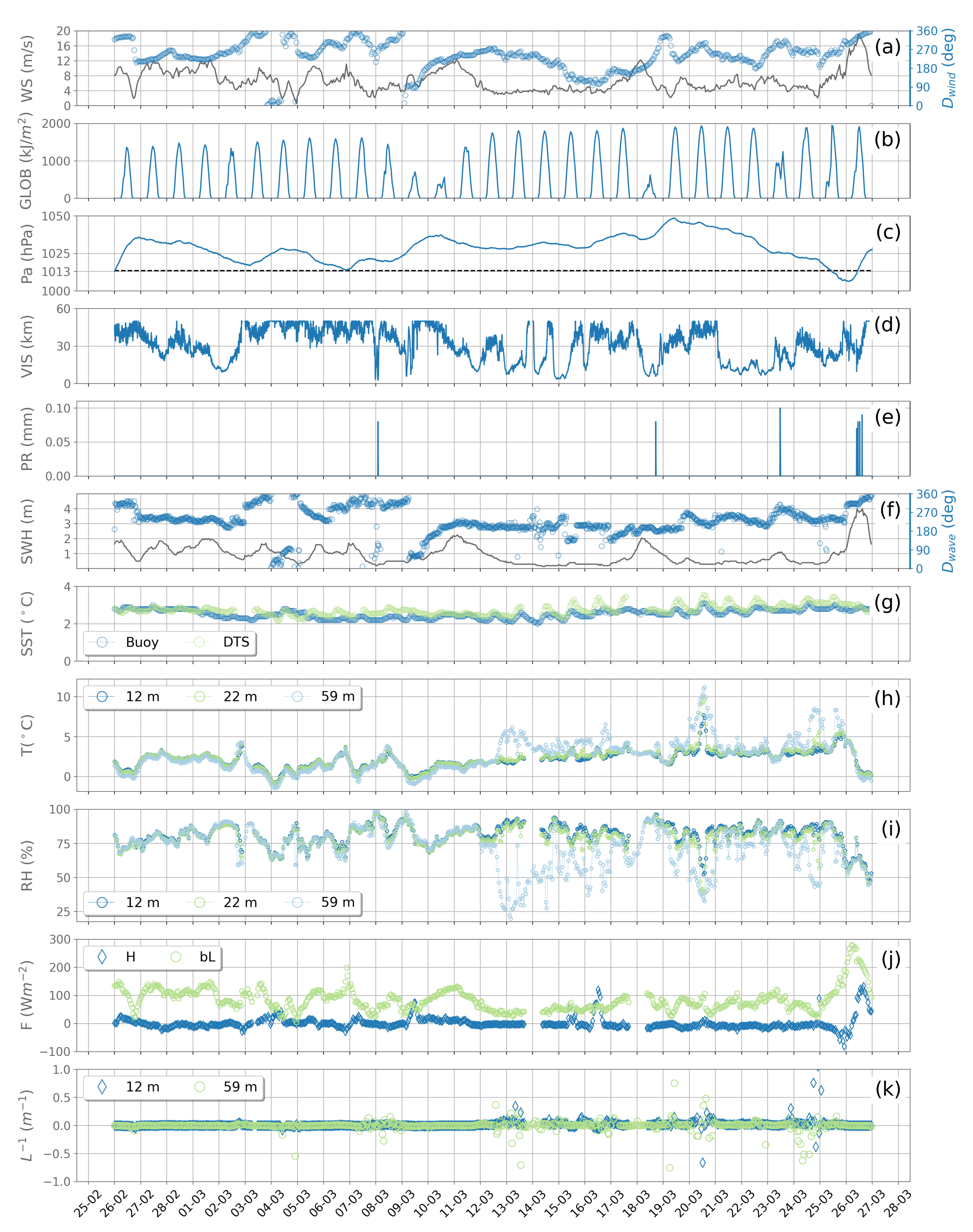
4.1. Weather Conditions

A high-pressure system persisted over northern Europe during the study period, moving from west to east. During the beginning of the study period, the high-pressure system was centred over Norway which allowed a warm Föhn wind to blow over the study area from the west. As the high-pressure system moved towards the east, the winds started to blow from the south and west, bringing warm, dry air from the western and southern Europe. High-pressure systems are usually associated with weaker winds and clearer skies. As a result, the March mean temperature in Utö was 2 $°$C warmer than the 1991–2020 average [37]. Towards the end of the study period, the high-pressure system moved away as a low-pressure system arrived; by the end of the study period, the low-pressure system was over Finland, with strong, cold winds blowing from the north.

Persistent ducting was observed with the coastal radar during a two-week period, from 12 to 25 March (Figure 4). The weather conditions during most of this period, with few exceptions, were favourable for ducting. The hourly averaged wind speed was $5.3\mathrm{m}{\mathrm{s}}^{-1}$ and the hourly averaged significant wave height was 0.6 m (Figure 5). Temperature and relative humidity measured at three heights (12, 22 and 59 m asl) showed stratification (inversion), with the temperature increasing and relative humidity decreasing with height (Figure 5). These gradients, together or separately, are preconditions to ducting and in fact partly coincide with the increases in total signal outside the radar horizon (Figure 4). In contrast, for the two weeks prior to the observed ducting, from the 26 February to the 11 March, wind speeds were generally greater, and the hourly averaged wind speed was $7.5\mathrm{m}{\mathrm{s}}^{-1}$ (Figure 5). In addition, the hourly averaged significant wave height was 1.1 m and no clear stratification was observed in temperature or relative humidity (Figure 5).

During the two-week ducting period, ducting was halted on the 18, 23 and 26 March when the total signal outside the standard horizon was near zero and significantly increased within the standard horizon (Figure 4). The total signal within the horizon was found to have a positive correlation with the significant wave height measured by the Northern Baltic Proper wave buoy. Moreover, the 18th and 26th storm events were characterised by strong winds, on the 18 March the maximum 30 min averaged wind speed was $13\mathrm{m}{\mathrm{s}}^{-1}$ and on the 26 March $19\mathrm{m}{\mathrm{s}}^{-1}$. The strong wind resulted in rough sea conditions; maximum significant wave heights measured by the Northern Baltic Proper buoy were 2 m on the 18th and 4 m on the 26th (Figure 5f). These storm events were strong enough to dismantle the established ducting conditions.

Sea surface temperature measured by the Northern Baltic Proper buoy (“c” in Figure 1) and the distributed temperature sensor at the Utö observatory (“1” and “2” in Figure 2) were between 2 and 4 $°$C during the study period (“g” in Figure 5). The atmosphere–sea temperature gradient was small during most of the study period and as such, the sensible heat flux was also small. During the reference period, the atmosphere–sea sensible heat flux measured at the Marine Research Station [21,38] varied between −25 and 25 $\mathrm{W}{\mathrm{m}}^{-2}$. During the ducting period when wind speeds were lower, the atmosphere–sea sensible heat flux was smaller and varied between −25 and 0 $\mathrm{W}{\mathrm{m}}^{-2}$.

The Baltic Sea ice winter of 2021–2022 was long (221 ice days) [39]. The maximum ice extent of 93,000 ${\mathrm{km}}^2$ was achieved on the 4 February, a couple of weeks before the chosen study period. Over the study period, the middle and inner archipelagos had a thin ice cover while the outer archipelago was ice-free (Figure 6). Sea ice was present in the northern parts of the standard horizon (Figure 6).

The wind profiles for the period between the 25 February and the 5 March show an average mixed layer height (MLH) of 93 m asl which is comparable to the MLH observations during previous winters on the Baltic Sea coast [35]. Starting from the 11 March, the MLH is very low and exceeds the lowest detection height of 16 m asl for only 33% of the time (Figure 7c). The data gaps from 5 until 10 March and on 18 March are due to instrumental reasons (Figure 7).

Furthermore, the period from 11 March onwards is also characterised by lower wind speeds compared to the period between 25 February and 5 March and low-level jets (LLJs) occur more frequently (Figure 7). LLJ, a local maximum in the vertical profile of horizontal wind speed, is a relatively common phenomenon at Utö (e.g., [40,41]). Typically, a local maximum in a wind profile is considered as a LLJ if the wind speed drops by 1 $\mathrm{m}{\mathrm{s}}^{-1}$ (e.g., [41]) or by 2 $\mathrm{m}{\mathrm{s}}^{-1}$ (e.g., [40]) above the maximum. In Figure 7c the local maxima with >1 $\mathrm{m}{\mathrm{s}}^{-1}$ drop in wind speed above the maximum are indicated as LLJ, but also weaker local maxima with 0.25–1 $\mathrm{m}{\mathrm{s}}^{-1}$ drop in wind speed are indicated. Notably, during the period when ducting was observed, LLJs were often present at or near the radar height (48 m asl). This indicates the existence of a layered structure that is decoupled from the surface at these elevations. During the earlier period, LLJs form at considerably higher altitudes of 150–250 m asl (Figure 7c).

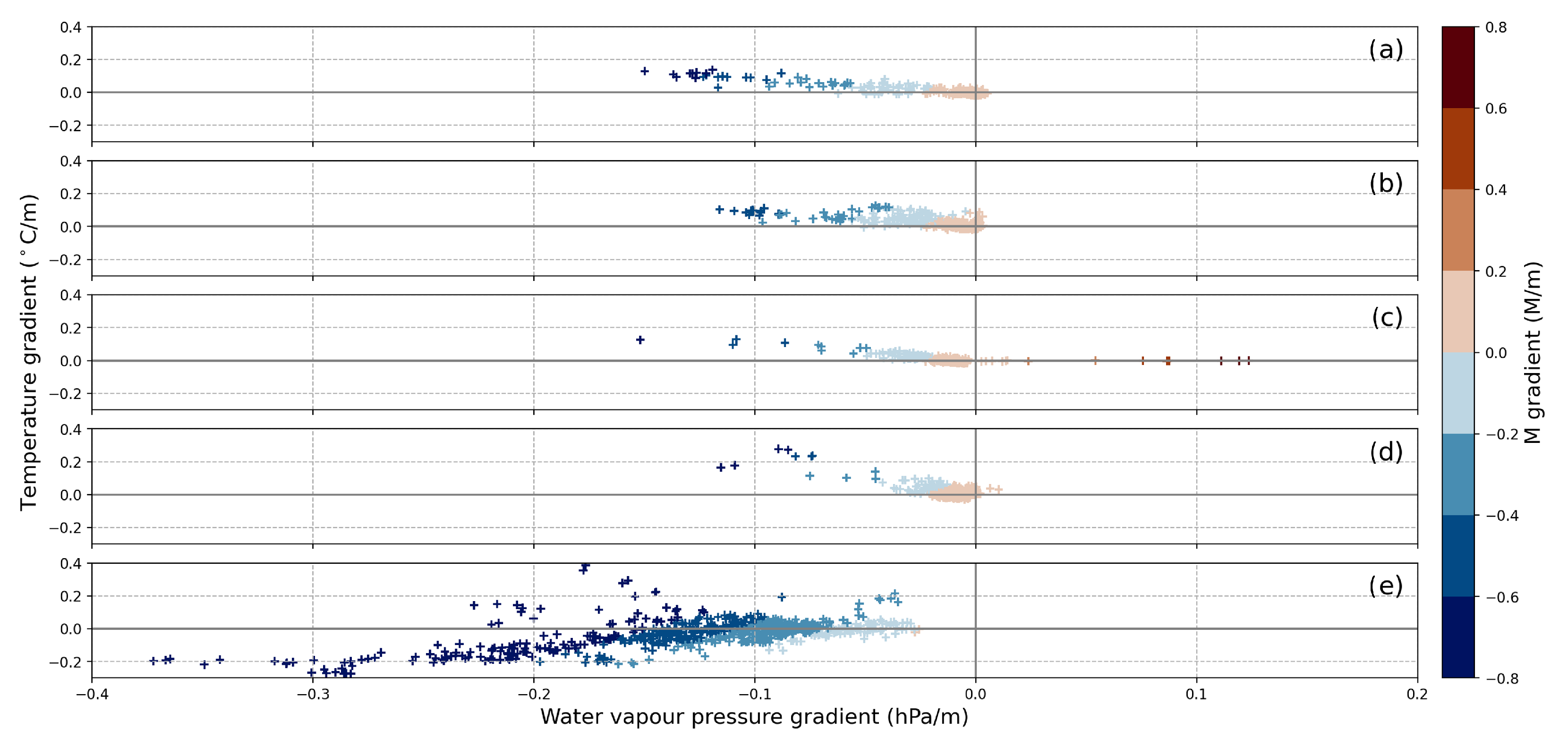
4.2. Analysis of the Ducting Period Based on the Modified Refractivity Gradients

The modified refractivity gradient (M-gradient), calculated from the Utö mast data and SST from the buoy, revealed that evaporation ducts occurred between 0 and 12 m asl over almost the whole four-week study period (Figure 8). It is worth noting that the height of the evaporation duct cannot be estimated based on the approximations of the surface temperature and humidity, and therefore, could be anywhere between 0 and 12 m in thickness. Babin et al. (1997) suggested that a 2 m vertical resolution is necessary to accurately model the evaporation duct height [5]. Furthermore, the thickness of the duct determines whether or not a signal of a specified frequency can be trapped in the duct [8]. Lower frequencies require deeper ducts and for X-band radars, the thickness needs to be at least 10 m for the signal to be trapped completely.

The M-gradient confirms the interpretation made from the mast temperature and relative humidity gradients, with ducts being present during the two-week period when the over-the-standard-horizon signal sum is greater than zero (Figure 8). Ducts in the top layer (32–59 m) are exceptionally strong when the radar signal sum increases from the 12 March to the 14 March, and weaker thereafter. In fact, out of the 424 data points, both agree 85% of the time. Unfortunately, measurements at 32 m are only available for the first three weeks of the study period. For the 22–59 m layer (over the whole study period, not shown in Figure 8), both the radar signal sum and the M-gradient are in agreement for 77% of the time. The same analysis was 43% for the 0–12 m layer and 66% for the 12–22 m layer. Overall, the negative M-gradient in the 22–59 m and 32–59 m layers can be considered a good forecast of over-the-standard-horizon detection for the Utö radar. For these two layers, on less than 10 occasions did the mast show a negative M-gradient that did not coincide with over-the-standard-horizon detection by the radar.

Under normal circumstances, such as from 26 February to 5 March, the horizontal wind speed increases with height (i.e., a positive wind speed difference above the radar height and a negative wind speed difference below the radar height (Figure 8c); whereas during the ducting period, the local wind speed maximum frequently occurs at or below the radar height (a negative wind speed difference above 50 m asl, Figure 8c). Previously, Liang et al. [42] reported ducting above marine LLJs, though in their case the LLJ was located hundreds of metres above sea level. This can be due to shear-induced mechanical turbulence resulting in a turbulent attenuation layer associated with temperature inversion and hydrolapse [42]. However, not all LLJs at the radar height coincide with ducting (Figure 8). Furthermore, in some cases (e.g., on the 14 March) strong ducting is observed when LLJs form just above the radar height at 100 m asl.

For the surface layer (0–12 m), the negative M-gradients were the result of a negative humidity gradient and a positive or negative temperature gradient with the humidity gradient being the more dominant feature (Figure 9). For the other layers, 12–22 m, 22–32 m and 32–59 m, decreasing humidity was accompanied by temperature inversions (Figure 9). A temperature inversion alone did not result in a negative M-gradient over the four-week study period. During the study period, a positive M-gradient was associated with a weak stratification in temperature and humidity (Figure 9).

4.3. Beginning of the Ducting Period

Before the ducting period began on the 12 March, the vertical profiles of temperature and relative humidity were near invariant with height from 12 to 59 m asl (Figure 10). At 15 UTC (17 local time) the temperature started to increase and the relative humidity decreased at the top measurement height (59 m), while the measurements below (at 32 m) remained constant, resulting in a negative modified refractivity gradient between 32 and 59 m (Figure 10). At lower heights (12 and 22 m), the relative humidity increased while temperature remained constant. At 18 UTC (20 local time), the top height temperature increased by 2.3 $°$C with relative humidity decreasing by 35%, while the 32 m temperature increased by 1.5 $°$C and relative humidity decreased by 18%, resulting in a negative modified refractivity gradient for the 12–22, 22–32 and 32–59 m heights. During the nine-hour period, the wind speed decreased from 6 to 2 $\mathrm{m}{\mathrm{s}}^{-1}$ and the sea–air temperature gradient was small, with sensible heat fluxes of $0\mathrm{W}{\mathrm{m}}^2$ while the latent heat flux decreased from 80 to $40\mathrm{W}{\mathrm{m}}^2$ (approximation). The wind direction was from west–south-west, i.e., from the open sea (Figure 7).

This leads us to consider three duct formation processes: subsidence due to the prevailing high-pressure system, horizontal advection of warm and dry air, and/or LLJ-related processes. Anticyclonic subsidence can result in an elevated duct, as high as 3 km at mid-latitudes [29]. In our case, at least the bottom of the duct is much lower, within 60 m from the surface. Horizontal advection of warm air over cooler sea surface is supported by the location downwind, within 100 km distance from the lee shore, as outlined by Turton [29]. As the ducting period coincided with a local horizontal wind maxima (LLJ) at the height of the radar (Figure 8), it poses an option for a third formation mechanism, a turbulent inversion. Similar conditions were observed by Liang et al. [42]. They observed a strong elevated ducting event (up to 38 M-units) where a dry air mass was over the wet marine atmospheric boundary layer and anticyclonic subsidence inversion was present. They found that, on a few occasions, the bottom of the trapping layer coincided with the maximum horizontal wind speed (LLJ) at 1600–2700 m. Liang et al. [42] concluded that jet-relevant ducts are generally weak but capped subsidence inversion and horizontal advection of dry air can enhance them [42]. In our case, the ducting event could have been caused by horizontal advection and be enhanced by the LLJ, as the LLJ only partly coincides with the M-profiles and the M-profiles are stronger when LLJ is present.

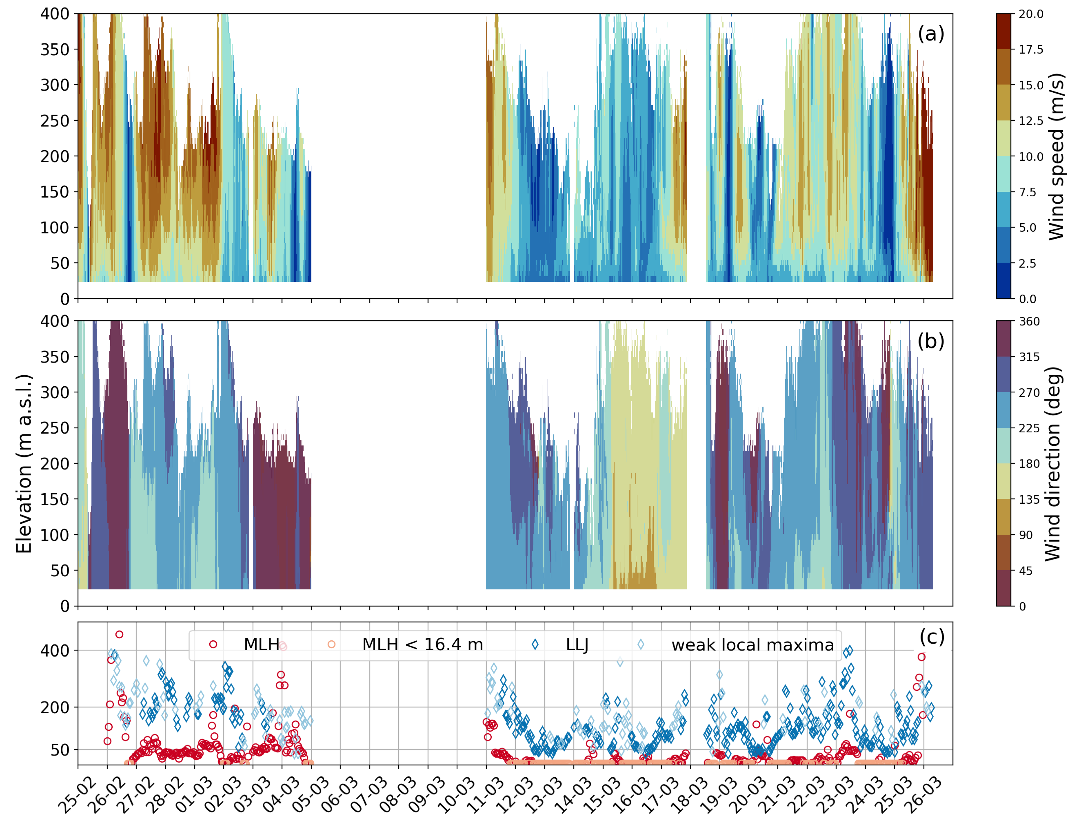
4.4. Analysis of the Ducting Period Based on the Coastal Radar

The composite of the maximum pixel value over the time period shows that the two-week event extended the radar horizon to 150 km in almost all directions (Figure 11). It appears, that without a pre-set limitation by the software, the radar horizon during the two-week period could have extended beyond 150 km. The shipping routes in particular are well covered, both in the open sea and within the Archipelago Sea. Signal propagation is usually physically limited by the islands in the Archipelago Sea. The composite shows that the radar signal propagation was only limited towards the Bothnian Sea (Northwest) where the intervening Archipelago Sea, with prominent islands and landforms, blocks most of the signal. The signal is also partly blocked to the east but the composite reveals that, during the two-week period, the radar signal was able to, at times, capture the shipping route to the coast, east of the radar.

It is worth noting that the visibility described by the composite is not achieved on a regular basis and such visibility has not simultaneously occurred in real life, at least not in record. However, the composite depicts the extent to which the radar was able to see during the exceptional two-week period and shows the extra capability that could be exploited if it is possible to accurately forecast or identify the conditions when extended visibility occurs.

The time series of the empirical indices (Figure 12) show that ducting, as a phenomenon, over the four-week period is not homogeneous over the radar area. The ducting events were strongest between the radar and the Hiiumaa coast (Figure 12); the ducting index was especially strong between the 12 and 15 March, and continuous in nature with the index being above zero for two consecutive days (13th and 14th), meaning the Hiiumaa coast was visible to the radar continuously during that time (Figure 12). The index also shows that for the strong four-day ducting event, the strength steadily increased from the 12th to the 14th and steadily decreased thereafter.

A similar ducting event was observed between the Swedish coast and Utö (Figure 12). The appearance of the time series of the two indices was similar, but the ducting index was stronger between Utö and Hiiumaa than between Utö and the Swedish coast. Although Hiiumaa is closer to the radar than the Swedish coast, the difference in strength is not explained by the distance as the index is normalised by the maximum. The difference is thought to be due to the Swedish coastal indicator area being at a lower elevation, where, for the Swedish coast to be detected by the radar, the duct would have to reach a lower elevation than for Hiiumaa. For Turku, the ducting index shows both shorter periods of ducting and longer periods of no ducting when compared to the other two locations (Figure 12).

The Turku index shows a peak on the 5 March that is not visible in the Hiiumaa index, and only a very minor peak is present in the Swedish coast index. In addition, there is a prominent peak in the signal sum within the 49–100 km range but not within the 100–150 km range (Figure 4). This means that, on the 5 March, ducting occurred in the direction of the Archipelago Sea but not towards the open sea. As other than ships and other moving targets between Utö and the Swedish coast and Utö and the Estonian coast, the 49–100 km range mainly includes signal from the islands of the Archipelago Sea. On the contrary, on the 27 February, the signal sum shows a peak in the 100–150 km range but not in the 49–100 km range, and there are peaks in the Hiiumaa and Swedish coast indices but not in the Turku index (Figure 4 and Figure 12). This means that ducting occurred over the open sea on the 27 February, but not in the Archipelago Sea.

5. Discussion

There is a need for fine-resolution, operational ducting forecasting. Ducting can be difficult to forecast over sea areas, as continuous measurements of the vertical profiles of refractivity are scarce and rely on expeditions or measurements at the coastline. In addition, using a single vertical profile requires the assumption of horizontal uniformity. Evaporation ducts, in particular, have a high spatial variability in the coastal region [43]. Utö has a unique set up, it is a small, remote island open to both the Archipelago and open sea. However, even with its remote location, it is inhabited throughout the year, which allows for the good up-keep of the instruments, and these measurements can be considered representative of the marine boundary layer stratification over the open sea. Our results showed that the measurements at Utö are representative of the over-the-horizon detection with the Utö coastal radar over the open sea, and vice versa. As such, the empirical ducting index shows promise for studies where numerical weather modelling-based ducting forecasts are evaluated, especially for areas as horizontally complicated as the Archipelago Sea where a point-sourced vertical profile of refractivity alone is not enough to capture the ducting conditions in the area.

The effects of the many islands of the Archipelago Sea are visible in the empirical ducting indices. Even though it was the closest chosen indicator location to the coastal radar (90 km), Turku was not continuously visible to the coastal radar, not even during the strongest ducting events. This is most likely due to the heterogeneity of the Archipelago Sea, where, to reach Turku, the signal has to propagate over several islands and islets, and over sea ice, rather than only above the open sea surface. The abrupt, horizontal changes in the surface, in terms of roughness, moisture and thermal forcing, affect the marine boundary layer structure [43], resulting in regions with variable propagation conditions. If the boundary layer is shallow, the topography can prevent horizontal flow and affect the boundary layer structure [43], and island wakes can also affect signal propagation [44]. This highlights the difficulty in producing a reliable ducting forecast for the Archipelago Sea. To accurately forecast and model ducting in the Archipelago Sea, especially in the inner archipelago, further studies are needed.

In addition, the coinciding of the LLJ height with the radar height at times during the ducting event poses opportunities for estimating the lower height of a trapping layer of a duct from the wind profile, important when estimating whether the radar would be affected by a duct. Tuononen et al. [40] found that the majority of LLJs at Utö occur below 150 m agl and are present evenly throughout the day during spring and winter. Since there is a connection between the observed ducting and LLJ height, the impact of LLJs on radio communications could be significant in Utö. Therefore, further studies of the relationship between ducting and LLJs, e.g., via modelling, is important. Liang et al. [42] highlighted the difficulty in modelling jet-relevant ducts due to the small scales of the wind-shear-produced eddies making them hard to accurately parameterise. For the complex nature of the Archipelago Sea and for the small-scale of the eddies, using large eddy simulation (LES) modelling to account for the complex marine boundary layer dynamics would be of interest.

Using coastal radar imagery for the ducting index comes with many benefits. It provides area-sensitive information on the relative strength, spread, duration and frequency of ducting events. For operational use, it provides a high-temporal-resolution, near real-time index if noise is taken into consideration without filtering, together with large spatial coverage at fine spatial and temporal resolutions. Coastal radars are also widely deployed, providing good coverage for coastal regions, with overlap between radars allowing the same area to be viewed from different directions, heights and angles. An index with these qualities is not achievable via other means. However, the success of the index in accurately observing the ducting events relies heavily on the height and angle of the radar in relation to the duct and target; therefore, the index is inherently uncertain, as would any other real-time index relying on a fixed-point measurement.

Encouraged by the results from the four-week study period, we are working on a continuation study where we will examine the annual variability of ducting based on the Utö coastal radar. At the Utö observatory, we have deployed additional two T-RH sensors at the heights of 4 and 7 m asl, to more accurately study evaporation ducts. We also plan to use the empirical ducting indices to perform an analysis of the numerical weather prediction model Harmonie-AROME in forecasting ducting.

6. Conclusions

In this study, we examined how measurements from the Utö observatory can be used to observe and analyse ducting events. We found that the negative M-gradient, based on vertical profiles of temperature and humidity, in the 22–59 m and 32–59 m layers can be considered a good forecast for the over-the-standard-horizon detection for the Utö coastal radar, and that the local maximum horizontal wind speed (LLJ) height often coincided with the coastal radar height over the study period. The spatial analysis revealed that ducting is not homogeneous over the radar area, and such areal indices are needed to support the point-source observations. The empirical ducting indices we developed provide information on the relative strength, frequency and occurrence of ducting in the radar area, and are not too computationally demanding for operational use. When applied to the whole coastal radar network on the Finnish coast, a large coverage over the Bothnian Bay, Bothnian Sea, Åland Sea, Archipelago Sea, Northern Baltic Proper and Gulf of Finland can be achieved, allowing for the operators in the area to have near real-time information on radar signal propagation and in general, radar network performance.

References

1. Linquist, T. Wave Propagation Models in the Troposphere for Long-Range UHF/SHF Radio Connections. Master’s Thesis, Karlstad University, Karlstad, Sweden, 2021. [Google Scholar]
2. Anderson, K. Radar measurements at 16.5 GHz in the oceanic evaporation duct. IEEE Trans. Antennas Propag. 1989, 37, 100–106. [Google Scholar] [CrossRef] [Green Version]
3. Reilly, J.; Dockery, G. Influence of evaporation ducts on radar sea return. IEEE Proc. F (Radar Signal Process.) 1990, 137, 80–88. [Google Scholar] [CrossRef]
4. Anderson, K. Radar detection of low-altitude targets in a maritime environment. IEEE Trans. Antennas Propag. 1995, 43, 609–613. [Google Scholar] [CrossRef] [Green Version]
5. Babin, S.M.; Young, G.S. A new model of the oceanic evaporation duct. J. Appl. Meteorol. 1997, 36, 193. [Google Scholar] [CrossRef]
6. Babin, S.M.; Dockery, G.D. LKB-Based Evaporation Duct Model Comparison with Buoy Data. J. Appl. Meteorol. 2002, 41, 434–446. [Google Scholar] [CrossRef]
7. Yang, C.; Wang, J.; Shi, Y. A Multi-Dimensional Deep-Learning-Based Evaporation Duct Height Prediction Model Derived from MAGIC Data. Remote Sens. 2022, 14, 5484. [Google Scholar] [CrossRef]
8. Dougherty, H.T.; Dutton, E.J. The Role of Elevated Ducting for Radio Service and Interference Fields; Technical Report TR-81-69; National Telecommunications and Information Administration (NTIA): Washington, DC, USA, 1981. [Google Scholar]
9. Huang, L.F.; Liu, C.G.; Wang, H.G.; Zhu, Q.L.; Zhang, L.J.; Han, J.; Zhang, Y.S.; Wang, Q.N. Experimental Analysis of Atmospheric Ducts and Navigation Radar Over-the-Horizon Detection. Remote Sens. 2022, 14, 2588. [Google Scholar] [CrossRef]
10. Wang, Q.; Alappattu, D.P.; Billingsley, S.; Blomquist, B.; Burkholder, R.J.; Christman, A.J.; Creegan, E.D.; de Paolo, T.; Eleuterio, D.P.; Fernando, H.J.S.; et al. CASPER: Coupled Air–Sea Processes and Electromagnetic Ducting Research. Bull. Am. Meteorol. Soc. 2018, 99, 1449–1471. [Google Scholar] [CrossRef]
11. Haus, B.K.; Ortiz-Suslow, D.G.; Doyle, J.D.; Flagg, D.D.; Graber, H.C.; MacMahan, J.; Shen, L.; Wang, Q.; Willams, N.J.; Yardim, C. CLASI: Coordinating Innovative Observations and Modeling to Improve Coastal Environmental Prediction Systems. Bull. Am. Meteorol. Soc. 2022, 103, E889–E898. [Google Scholar] [CrossRef]
12. Wang, S.; Yang, K.; Shi, Y.; Yang, F.; Zhang, H.; Ma, Y. Prediction of Over-the-Horizon Electromagnetic Wave Propagation in Evaporation Ducts Based on the Gated Recurrent Unit Network Model. IEEE Trans. Antennas Propag. 2023, 71, 3485–3496. [Google Scholar] [CrossRef]
13. Wagner, N.K. An analysis of radiosonde effects on the measured frequency of occurrence of ducting layers. J. Geophys. Res. (1896–1977) 1960, 65, 2077–2085. [Google Scholar] [CrossRef]
14. Ao, C.O. Effect of ducting on radio occultation measurements: An assessment based on high-resolution radiosonde soundings. Radio Sci. 2007, 42. [Google Scholar] [CrossRef] [Green Version]
15. Bech, J.; Codina, B.; Lorente, J.; Bebbington, D. Monthly and Daily Variations of Radar Anomalous Propagation Conditions: How “Normal” Is Normal Propagation? Copernicus GmbH: Delft, The Netherlands, 2002; pp. 35–39. [Google Scholar]
16. Bech, J.; Codina, B.; Lorente, J. Forecasting weather radar propagation conditions. Meteorol. Atmos. Phys. 2007, 96, 229–243. [Google Scholar] [CrossRef]
17. Grabner, M.; Kvicera, V. Refractive Index Measurement at TV Tower Prague. Radioengineering 2003, 12, 5–7. [Google Scholar]
18. Falodun, S.; Ajewole, M. Radio refractive index in the lowest 100-m layer of the troposphere in Akure, South Western Nigeria. J. Atmos. Sol.-Terr. Phys. 2006, 68, 236–243. [Google Scholar] [CrossRef]
19. Adediji, A.; Ajewole, M.; Falodun, S. Distribution of radio refractivity gradient and effective earth radius factor (k-factor) over Akure, South Western Nigeria. J. Atmos. Sol.-Terr. Phys. 2011, 73, 2300–2304. [Google Scholar] [CrossRef]
20. Miettunen, E.; Tuomi, L.; Myrberg, K. Water exchange between the inner and outer archipelago areas of the Finnish Archipelago Sea in the Baltic Sea. Ocean. Dyn. 2020, 70, 1421–1437. [Google Scholar] [CrossRef]
21. Laakso, L.; Mikkonen, S.; Drebs, A.; Karjalainen, A.; Pirinen, P.; Alenius, P. 100 years of atmospheric and marine observations at the Finnish Utö Island in the Baltic Sea. Ocean Sci. 2018, 14, 617–632. [Google Scholar] [CrossRef] [Green Version]
22. Karvonen, J.; Simila, M.; Lehtiranta, J. SAR-based estimation of the baltic sea ice motion. In Proceedings of the 2007 IEEE International Geoscience and Remote Sensing Symposium, Barcelona, Spain, 23–27 July 2007; pp. 2605–2608. [Google Scholar] [CrossRef]
23. SITAC of the Copernicus Marine Service. Quality Information Document; Copernicus Marine Service; European Union: Brussels, Belgium, 2022. [Google Scholar] [CrossRef]
24. Lensu, M.; Heiler, I.; Karvonen, J. Range compensation in pack ice imagery retrieved by coastal radars. In Proceedings of the 2014 IEEE/OES Baltic International Symposium (BALTIC), Tallinn, Estonia, 27–29 May 2014; pp. 1–5. [Google Scholar] [CrossRef]
25. Pearson, G.; Davies, F.; Collier, C. An Analysis of the Performance of the UFAM Pulsed Doppler Lidar for Observing the Boundary Layer. J. Atmos. Ocean. Technol. 2009, 26, 240–250. [Google Scholar] [CrossRef]
26. Hirsikko, A.; O’Connor, E.J.; Komppula, M.; Korhonen, K.; Pfüller, A.; Giannakaki, E.; Wood, C.R.; Bauer-Pfundstein, M.; Poikonen, A.; Karppinen, T.; et al. Observing wind, aerosol particles, cloud and precipitation: Finland’s new ground-based remote-sensing network. Atmos. Meas. Tech. 2014, 7, 1351–1375. [Google Scholar] [CrossRef] [Green Version]
27. Vakkari, V.; Manninen, A.J.; O’Connor, E.J.; Schween, J.H.; van Zyl, P.G.; Marinou, E. A novel post-processing algorithm for Halo Doppler lidars. Atmos. Meas. Tech. 2019, 12, 839–852. [Google Scholar] [CrossRef] [Green Version]
28. Browning, K.A.; Wexler, R. The Determination of Kinematic Properties of a Wind Field Using Doppler Radar. J. Appl. Meteorol. Climatol. 1968, 7, 105–113. [Google Scholar] [CrossRef]
29. Turton, J.; Bennetts, D.; Farmer, S. An introduction to radio ducting. Meteorol. Mag. 1988, 117, 245–254. [Google Scholar]
30. ITU. The Radio Refractive Index: Its Formula and Refractivity Data, Recommendation ITU-R P.453-6; Technical Report; International Telecommunication Union: Geneva, Switzerland, 2019. [Google Scholar]
31. Grabner, M.; Kvicera, V. Atmospheric Refraction and Propagation in Lower Troposphere. In Electromagnetic Waves; Zhurbenko, V., Ed.; IntechOpen: Rijeka, Croatia, 2011; Chapter 7. [Google Scholar] [CrossRef] [Green Version]
32. Patterson, W.L. Chapter 26: The Propagation Factor Fp in the radar equation. In Radar Handbook, 3rd ed.; Skolnik, M.I., Ed.; McGraw-Hill: New York, NY, USA, 2008; pp. 1290–1315. [Google Scholar]
33. Palmer, A.J.; Baker, D.C. A Novel Simple Semi-Empirical Model for the Effective Earth Radius Factor. IEEE Trans. Broadcast. 2006, 52, 557–565. [Google Scholar] [CrossRef]
34. Copernicus Land Monitoring Service. EU-DEM. Copernicus Land Monitoring Service: European Union. 2014. Available online: https://land.copernicus.eu/imagery-in-situ/eu-dem. (accessed on 6 June 2023).
35. Vakkari, V.; O’Connor, E.J.; Nisantzi, A.; Mamouri, R.E.; Hadjimitsis, D.G. Low-level mixing height detection in coastal locations with a scanning Doppler lidar. Atmos. Meas. Tech. 2015, 8, 1875–1885. [Google Scholar] [CrossRef] [Green Version]
36. O’Connor, E.J.; Illingworth, A.J.; Brooks, I.M.; Westbrook, C.D.; Hogan, R.J.; Davies, F.; Brooks, B.J. A Method for Estimating the Turbulent Kinetic Energy Dissipation Rate from a Vertically Pointing Doppler Lidar, and Independent Evaluation from Balloon-Borne In Situ Measurements. J. Atmos. Ocean. Technol. 2010, 27, 1652–1664. [Google Scholar] [CrossRef] [Green Version]
37. FMI. Lämpötila-ja Sadekarttoja Vuodesta 1961; FMI: Helsinki, Finland, 2023. [Google Scholar]
38. Honkanen, M.; Tuovinen, J.P.; Laurila, T.; Mäkelä, T.; Hatakka, J.; Kielosto, S.; Laakso, L. Measuring turbulent CO2 fluxes with a closed-path gas analyzer in a marine environment. Atmos. Meas. Tech. 2018, 11, 5335–5350. [Google Scholar] [CrossRef] [Green Version]
39. FMI. Jäätalvi 2021–2022 Oli Pitkä ja Leuto; FMI: Helsinki, Finland, 2022. [Google Scholar]
40. Tuononen, M.; O’Connor, E.J.; Sinclair, V.A.; Vakkari, V. Low-Level Jets over Utö, Finland, Based on Doppler Lidar Observations. J. Appl. Meteor. Climatol. 2017, 56, 2577–2594. [Google Scholar] [CrossRef]
41. Hallgren, C.; Arnqvist, J.; Ivanell, S.; Körnich, H.; Vakkari, V.; Sahlée, E. Looking for an Offshore Low-Level Jet Champion among Recent Reanalyses: A Tight Race over the Baltic Sea. Energies 2020, 13, 3670. [Google Scholar] [CrossRef]
42. Liang, Z.; Ding, J.; Fei, J.; Cheng, X.; Huang, X. Maintenance and Sudden Change of a Strong Elevated Ducting Event Associated with High Pressure and Marine Low-Level Jet. J. Meteorol. Res. 2020, 34, 1287–1298. [Google Scholar] [CrossRef]
43. Brooks, I.M. Air-sea interaction and spatial variability of the surface evaporation duct in a coastal environment. Geophys. Res. Lett. 2001, 28, 2009–2012. [Google Scholar] [CrossRef] [Green Version]
44. Jiang, Q.; Wang, Q.; Gaberšek, S. Mesoscale Variability of Surface Ducts During Santa Ana Wind Episodes. J. Geophys. Res. Atmos. 2022, 127, e2022JD036698. [Google Scholar] [CrossRef]
45. Crameri, F. Scientific Colour Maps; Zenodo: Meyrin, Switzerland, 2021. [Google Scholar] [CrossRef]
46. Crameri, F.; Shephard, G.; Heron, P. The misuse of colour in science communication. Nat. Commun. 2020, 11, 5444. [Google Scholar] [CrossRef]
Figure 1. (a) Location of the Utö coastal radar on the island of Utö at the southern edge of the Archipelago Sea. The circles depict the radar standard horizon and extended horizons. (b) Close up of the standard horizon. Locations of the Korppoo weather radar and two nearby wave and SST buoys included.
Remotesensing 15 02989 g001
Figure 2. Observations at Utö. For details and location, see Table 1 and Figure 1.
Remotesensing 15 02989 g002
Figure 3. (a) Cross-sections from Utö to the three indicator locations Turku, Swedish coast and Hiiumaa on a map with the radar standard horizon and extended horizons. Topography panels matching the cross-sections from Utö to (b) Hiiumaa, (c) Swedish coast and (d) Turku with the target locations in each subplot indicated with dashed red vertical lines.
Remotesensing 15 02989 g003
Figure 4. Signal sum within the standard radar horizon (<49 km) and beyond the standard radar horizon (49–100 km and >100 km). Signal sum beyond 49 km is zero unless ducting occurs. Within the standard radar horizon, the signal sum changes mainly due to sea surface roughness, i.e., waves.
Remotesensing 15 02989 g004
Figure 5. Weather conditions over the four-week study period, from 26 February to 26 March 2022, where (a) wind speed ( m s 1 ) as a grey line and wind direction ( ° ) at 19 m (25 m asl) as blue circles, (b) global radiation ( kJ m 2 ), (c) air pressure (hPa) in blue with 1013 hPa denoted as a black dashed line, (d) visibility (m), (e) precipitation (mm), (f) significant wave height (m) as a grey line and wave direction ( ° ) as blue circles, (g) sea surface temperature ( ° C) both from the Northern Baltic Proper wave buoy in blue and distributed temperature sensor (DTS) measurements in green, (h) temperature ( ° C) at heights 12, 22 and 59 m in dark blue, green and light blue, respectively, (i) relative humidity (%) at heights 12, 22 and 59 m in dark blue, green and light blue, respectively, (j) sensible heat (H) and calculated latent heat (bL) fluxes (Wm 2 ) in blue and green, respectively, and (k) inverse Monin–Obukhov length (m 1 ) at heights 12 and 59 m, in blue and green, respectively.
Remotesensing 15 02989 g005
Figure 6. Sea ice occurrence (%) over the four-week study period, from 26 February to 26 March 2022. Note: does not consider the ice type, simply if sea ice was present. The Utö coastal radar is shown as the red square in the middle.
Remotesensing 15 02989 g006
Figure 7. Halo lidar vertical profile measurements over the four-week study period, from 26 February to 26 March 2022. (a) shows the wind speed ( m s 1 ), (b) the wind direction ( ° ) and (c) the mixed layer height (MLH) and low-level jet (LLJ) height (m) asl. Gaps are missing data.
Remotesensing 15 02989 g007
Figure 8. (a) Signal sum beyond the standard radar horizon (>49 km). The sum is zero unless ducting occurs. (b) Modified refractivity gradient (dM/dh) for the layers 0–12, 12–22, 22–32, 22–59 and 32–59 m. Note that the values for the 0–12 m layer are based on SST and an assumption of 100% humidity over the sea surface and should only be considered as a rough estimate. Ducting occurs when the gradient is negative (indicated by a blue colour). (c) Wind speed—wind speed at the height of the radar.
Remotesensing 15 02989 g008
Figure 9. Gradients in water vapour pressure, temperature and modified refractivity for layers at (a) 32–59 m, (b) 22–59 m, (c) 22–32 m, (d) 12–22 m and (e) 0–12 m.
Remotesensing 15 02989 g009
Figure 10. Hourly means of vertical profiles of temperature (top panel), relative humidity (middle panel) and modified refractivity (bottom panel) from 12 UTC (14 local time) on the left to 20 UTC (22 local time) on the right, for the 12 March 2022. Hour 12 profiles shown in grey and the difference to the hour 12 profile is shown as a blue shadow.
Remotesensing 15 02989 g010
Figure 11. A composite image depicting the maximum pixel value (0–255) observed during the two-week ducting period, from the 12 March to the 26 March 2022. The y- and x-axes are the coordinates, each side corresponding to 300 km. Radar is in the middle of the composite, on the island of Utö. The standard horizon (<49 km) is indicated by the shaded circle.
Remotesensing 15 02989 g011
Figure 12. An empirical ducting index for the three chosen areas: (a) Hiiumaa, Estonia, 104 km from the radar, (b) coastline of Sweden, 143 km from the radar, and (c) Turku, Finland, 90 km from the radar.
Remotesensing 15 02989 g012