Article

Spatio-Temporal Variability Analysis of Vegetation Dynamics in China from 2000 to 2022 Based on Leaf Area Index: A Multi-Temporal Image Classification Perspective

1
Center for GeoData and Analysis, State Key Laboratory of Remote Sensing Science, Faculty of Geographical Science, Beijing Normal University, Beijing 100875, China
2
School of Land Science and Technology, China University of Geosciences, Beijing 100083, China
3
Key Laboratory of High Confidence Software Technologies, Peking University, Beijing 100871, China
4
School of Linkong Economics and Management, Beijing Institute of Economics and Management, Beijing 100102, China
*
Author to whom correspondence should be addressed.
Remote Sens. 2023, 15(12), 2975; https://doi.org/10.3390/rs15122975
Submission received: 10 May 2023 / Revised: 24 May 2023 / Accepted: 2 June 2023 / Published: 7 June 2023

Abstract

:
Leaf Area Index (LAI) is one of the most important biophysical parameters of vegetation, and its dynamic changes can be used as a reflective indicator and differentiation basis of vegetation function. In this study, a VCA–MLC (Vertex Component Analysis–Maximum Likelihood Classification) algorithm is proposed from the perspective of multi-temporal satellite LAI image classification to monitor and quantify the spatial and temporal variability of vegetation dynamics in China since 2000. The algorithm extracts the vegetation endmembers from 46 multi-temporal images of MODIS LAI in 2011 without the aid of other a priori knowledge and uses the maximum likelihood classification method to select the categories that satisfy the requirements of the number of missing periods, absolute distance, and relative distance for the rest pixels to be classified, ultimately dividing the vegetation area of China into 10 vegetation zones called China Vegetation Functional Zones (CVFZ). CVFZ outperforms MCD12Q1 and CLCD land cover datasets in the overall differentiation of vegetation functions and can be used synergistically with other land cover datasets. In this study, CVFZ is used to cut the constant vegetation-type pixels of MCD12Q1 during 2001–2022. The results of the LAI mean time series decomposition of each subregion using the STL (Seasonal-Trend Decomposition based on Loess) method show that the rate of vegetation greening ranges from 9.02 × 10⁻⁴ m2m−2yr−1 in shrubland subregions to 2.34 × 10⁻² m2m−2yr−1 in savanna subregions. In relative terms, the average greening speed of forests is moderate, and savannas tend to have the fastest average greening speed. The greening speed of grasslands and croplands in different zones varies widely. In contrast, the average greening speed of shrublands is the slowest. In addition, CVFZ detected grasslands with one or two phenological cycles, broadleaf croplands with one or two phenological cycles, and shrublands with no apparent or one phenological cycle.

Graphical Abstract

1. Introduction

Vegetation plays a significant role in the terrestrial–atmospheric water cycle by transpiring and has a considerable impact on energy flow and carbon cycles in the Earth’s system [1]. The Leaf Area Index (LAI) is a crucial biophysical parameter of vegetation [2]. It is an essential input parameter for vegetation dynamics, phenology monitoring, crop yield estimation, and climate model [3,4,5,6], and LAI can also detect changes in climate and land use/cover [6,7].
In recent decades, numerous studies have been conducted using satellite LAI to examine vegetation’s response to climate change [8,9]. Studies by Vremec et al. [10] and Cook et al. [11] confirmed that CO2 primarily affects vegetation by modifying its stomatal resistance, resulting in fertilization effects and increased evaporation. Lawal et al. [12] and Zhang et al. [13] studied vegetation dynamics (recovery, migration, and extinction) under drought and varying climatic conditions, rainfall, and altitude. Simultaneously, these studies identified that these drivers have diverse effects on vegetation dynamics at the regional scale. Jiao et al. [14] and Holm et al. [15] studied the distinct effects of drought on species composition and carbon sink storage in the central and western Amazon forests, revealing that deep rooting is a leading cause of greening during severe drought. Yang et al. [16] and Qiu et al. [17] identified different driving patterns of vegetation climate under various altitude gradients of the Qinghai–Tibet Plateau, and vegetation growth in relatively high-altitude areas is determined by growing season precipitation and atmospheric CO2 concentrations, while relatively low altitudes are dominated by growing precipitation. Climate change has a profound impact on vegetation dynamics, hydrological cycles, and ecosystem productivity globally [18,19].
Consequently, changes in vegetation dynamics have a biophysical effect on the local and even global climate, resulting in positive or negative feedback on the climate system [20]. An increase in vegetation LAI has the potential to affect soil moisture, precipitation, and increase global terrestrial carbon sinks [21,22]. Furthermore, it can alter surface albedo and evapotranspiration, leading to increased warming in northern regions and slowed warming in local tropical regions [23,24].
Numerous studies have reported a nearly 50% increase in greening trends for global vegetation since the 1980s [25,26,27]. Moreover, the greening differences among various vegetation species have been widely studied. Caracciolo et al. [28] and Andela et al. [29] found that forests, which have access to deeper aquifers and dominate over grasslands in bare landscaping, exhibit the main climatic factor in mixed forests, evergreen needleleaf forests, and deciduous broadleaf forests as temperature, while grasslands are more impacted by precipitation, temperature, and solar radiation [30]. The differences between grasslands and forests in mountainous or polar regions have also received attention in recent greening [2,31]. Shrublands and tundra at high latitudes have been prioritized over forest greening [32] in which the annual carbon increase in tundra greening is associated with water loss at the weakest; yet, it has produced positive feedback on Arctic warming [33,34].
Most vegetation-to-vegetation difference studies rely on land cover maps [30,32,35]. The main land cover products to date have used random forests, decision trees, and some machine learning methods to achieve high classification accuracy and efficiency [36,37,38,39]. They usually distinguish only vegetation types or provide the proportion of major vegetation types [40,41].
However, there is a lack of research on the differences between vegetation in the corresponding vegetation functional areas. For instance, the adaptive ability of low-latitude functional vegetation during migration is relatively inferior to that of high-latitude functional vegetation and exhibits greater LAI variability [31]. Nonetheless, low-latitude functional vegetation, especially in tropical monsoon and rainforest climate areas, has generally higher forest biomass densities in tropical rainforest climate zones than high-latitude functional vegetation [42]. Moreover, the study showed forests and grasslands with different vegetation functions had high spatial heterogeneity in the four vegetation parameters of gross primary productivity (GPP), net primary productivity (NPP), LAI, and vegetation cover (FVC). This was manifested by different rates of vegetation recovery, vegetation productivity, and ecosystem stability [43]. Mainly influenced by climatic drivers, the differences in urban forest functions are also reflected in many aspects such as green density, green intensity, and biodiversity [44]. Linking vegetation characteristics obtained from remote sensing to vegetation functions can effectively improve spatial distribution ecological modeling and assessment [45].
Hence, it is essential to utilize zoning specifically for vegetation functions to investigate the spatio-temporal variability of vegetation dynamics and further explore the correlation between the vegetation dynamics and the underlying drivers. Since the dynamic change of LAI can be used as a reflection index and differentiation basis for vegetation function [46], this study suggests a new approach to divide vegetation pixels into distinct vegetation functional areas. The algorithm used in this study is an algorithm extended in hyperspectral image classification to multi-temporal image classification. The implementation process takes China as an example, and the derivative product is named China Vegetation Functional Zones (CVFZ).
Furthermore, several prior studies have only been conducted at a single-pixel or small-area scale [47,48,49]. However, given that most long-term changes in vegetation dynamics are nonlinear, non-stationary, and complex [50,51], analysis focused solely on a single-pixel or small-area scale may inaccurately reflect or even underestimate vegetation’s response mechanism to climate change [52,53]. To accurately analyze vegetation behavior that is difficult to detect using terrestrial methods [54,55], studies carried out at large-scale spatial scales for ecosystems and biodiversity and considering the importance of diagnosing and responding to global climate change are necessary.
In this study, we investigate the spatio-temporal variability of vegetation dynamics in China from 25 June 2000 to 25 June 2022, as reflected by satellite LAI, through the classification perspective of multi-temporal images. The average LAI in China during this period was 1.04 m2m−2 with a standard deviation of 1.00 m2m−2 (Figure 1). Our study is divided into two main parts. The first part involves the production and validation of CVFZ, which is based on Vertex Component Analysis–Maximum Likelihood Classification (VCA–MLC). The vegetation pixels in China are divided into 10 regions through CVFZ, and cross-validation with other land cover classification maps indicates the need for the functional zoning of vegetation. In the second part, we conduct a large-area scale analysis, using CVFZ to refine other land cover classification maps (we use MCD12Q1 as an example in this paper) and obtain a more detailed land cover classification map (MCD-CVFZ) that can distinguish vegetation functions. Finally, we extract the subregion LAI mean time series according to the MCD-CVFZ and separately analyze the annual and intra-annual fluctuations of vegetation dynamics through Seasonal-Trend Decomposition based on the Loess (STL) method.
The rest of our paper is arranged as follows: In Section 2, we introduce the datasets and methods used in this study, including the VCA–MLC algorithm, three validation indicators of the vegetation functional area, and the STL method. In Section 3, we present the results of the production, evaluation, and application of CVFZ. We discuss the potential advantages of CVFZ and the spatial variability of vegetation dynamics revealed by CVFZ in Section 4. Additionally, we discuss the connection between vegetation dynamics and other drivers in Section 4.

2. Materials and Methods

2.1. Satellite Data

The research analysis was based on the C61 version of the MODIS product, which is similar in format to the C6 product. However, the C61 version has been improved by satellite calibration and polarization methods, making it more advanced than the previous C6 version. Our analysis relied on LAI from the MOD15A2H dataset provided by NASA EOSDIS LP DAAC (https://lpdaac.usgs.gov/products/mod15a2hv061, accessed on 14 February 2023). This dataset provides eight-day maximum synthesis of LAI and FPAR products from 2000 years ago to the present, with a spatial resolution of 500 m [56,57]. The sources of uncertainty in the MOD15A2H dataset are mainly reflectance data, canopy aggregation effects, and inversion models [58]. However, it has undergone more comprehensive and extensive validation among many LAI products, and its use to study LAI time series over a 22-year period is motivated by considerations of ensuring data consistency and continuity [59,60]. Land cover datasets come from MCD12Q1 provided by NASA EOSDIS LP DAAC (https://lpdaac.usgs.gov/products/mcd12q1v061, accessed on 16 February 2023), and CLCD (Annual China Land Cover Dataset) were provided by the team of professors Yang Jie and Huang Xin of Wuhan University (https://zenodo.org/record/5816591, accessed on 21 February 2023). MCD12Q1 provides a global land cover map with a spatial resolution of 500 m for six different land cover legends for each year from 2001 to the present [41]. The annual LAI classification scheme specified in the LC type3 band was used to divide the land cover into 8 types, which is commonly used with MOD15A2H [61,62]. In this study, only natural ecosystems with an unchanged vegetation type between 2001 and 2022 were preserved (MCD-unchanged) as the object cut by CVFZ. Changes in vegetation type can significantly affect the degree of response of plants to climate change [63]; therefore, preserving the unchanged vegetation type is important. CLCD provides year-to-year land cover data from 1985 to the present, with a spatial resolution of 30 m [64]. CLCD from 2011 (CLCD-2011), MCD12Q1 from 2011 (MCD-2011), and the MCD-unchanged were used in cross-evaluation with CVFZ. All rasters were resampled to 2000 m and reprojected to the same coordinate system to ensure they were of the same size, which was 2884 × 3743.

2.2. Extraction and Selection of Vegetation Endmembers for China

VCA (Vertex Component Analysis) is an endmember extraction algorithm that has been utilized for hyperspectral remote sensing image classification [65,66,67,68]. The computational complexity of VCA is the lowest among the methods for endmember extraction, and the performance also tends to be optimal compared to non-intelligent optimization algorithms such as N-FINDR and PPI [69]. This study employed VCA to extract Chinese vegetation endmembers. Vegetation endmembers were extracted from C61 MODIS15A2H LAI using 46-phase multi-temporal images of vegetation pixels only from 2011 produced by the main algorithm (called MOD-2011), thus effectively preserving a substantial portion of information on annual vegetation dynamics over 2000–2022 while conserving computing and storage resources. First, the set of all pixels in MOD-2011 was combined into a monomorphic body resulting in
S x = x R m : x = M α ,   1 T α = 1 ,   α 0
where M is the confusion matrix of all endmembers, 1 is an all-one vector of L × 1 dimensions, and α is the abundance transpose vector containing the fraction of each endmember. Assuming the existence of pure pixels, the endmembers are located at the vertices of the monomorphic body. Sx is projected into the hyperplane xTu = 1 to obtain a monomorphic body in the direction of an orthogonal subspace, where u is to ensure that there are no observation vectors orthogonal to the hyperplane.
S p = y R m : y = x x T u ,   x S x
Next, the observation data are projected to Sp, and the pixel with the largest projection distance value is calculated as the endmember. Iterative calculations are then performed until all vegetation endpoints are found. Due to the randomness inherent in the projection process, there is a degree of variation in the extraction results for each vegetation end element beyond the first. To reduce this randomness, the extraction process was repeated 1000 times. Each cycle resulted in only 2 vegetation endmembers with no missing phases. Table 1 shows that the final endmembers are selected with a probability of occurrence ( P o c c u r r e n c e ) greater than 1%.

2.3. Creating China Vegetation Functional Zones (CVFZ) Based on the Selected Endmembers

After selecting the vegetation endmembers, pixels in MOD-2011 with more than 20 periods missing were filtered out to determine the category of the rest pixels, which removed 6.13% of the total number of pixels. The n-dimensional vector expression of each pixel position in the coordinate system is obtained:
X = x 1 , x 2 , x m T
The distance (D) between two multi-temporal pixels was characterized using a compound distance constructed by combining the Euclidean distance and the spectral shape angle cosine. The spectral shape angle cosine is independent of the gain coefficient of the LAI multi-temporal image and ranges between 0 and 1, reflecting the similarity of the two multi-temporal pixels. This helps to address the limitation of using only Euclidean distance, which cannot fully reflect the change in the pixel LAI time series. By combining the two spectral characteristics of time phase amplitude and time phase shape, the accuracy of similarity measurement between multi-temporal pixels is improved [70,71]. D can be expressed as follows:
D = i = 1 m x i x i 2 m 1 i = 1 m x i x i i = 1 m x i 2 i = 1 m x i 2
where 1 minus the angular cosine of the spectral shape is used to unify the increase or decrease in the two distance indicators, further obtaining the absolute distance DA and the relative distance DR.
D A = D p i x e l z e r o s D e n d m e m b e r z e r o s
D R = D p i x e l e n d m e m b e r
where zeros is an all-one vector of 1 × 46 dimensions. DA represents the absolute distance between the pixel to be classified and the endmember, and DR represents the relative distance between them.
The MLC (Maximum Likelihood Classification) algorithm achieves the effect of classification by substituting the image to be classified into the determined classification function on a pixel-by-pixel basis [72]. This algorithm builds upon Xu et al. [73] by using the idea of equidistant loss to adjust the distance between samples with relative distance constraints. Thus, absolute distances are added to intervene in the classification process of vegetation pixels. The algorithm calculates the DR of each pixel to 10 endmembers in turn. If DR is the smallest and DA is not greater than the Threshold, the pixel belongs to the category. The existence of a Threshold results in not all pixels being classified. The above classification process is called the VCA–MLC algorithm (Figure 2). The derivative product is called the Chinese Vegetation Functional Zones (CVFZ).

2.4. Optimization and Validation of the Created CVFZ

As there is no identifiable vegetation functional area endmember to reference, it is difficult to evaluate the performance of the VCA–MLC algorithm using indicators such as root mean square–Signature Angle Error (rms–SAE). Therefore, the algorithm’s performance is indirectly evaluated by assessing the discrimination effect of CVFZ on vegetation function, with the key indicators for evaluating image classification accuracy being interclass distance and in-class distance [74]. Missing rate (MR), interclass distance (D1), in-class distance (D2), and discrimination (D3) are proposed to optimize and validate CVFZ. D1, D2, and D3 are also used to evaluate MCD-2011, CLCD-2011, MCD-unchanged, and MCD-CVFZ. These formulas are as follows:
M R = 1 k = 0 9 c k c
D 1 = k 1 = 0 9 k 2 = k 1 + 1 9 D m e a n k 1 m e a n k 2 k 1 = 0 9 k 2 = k 1 + 1 9 1
D 2 = k = 0 9 j = 1 c k D m e a n k p i x e l k j k = 0 9 j = 1 c k 1
D 3 = D 1 D 2
where k is the category in which the pixel belongs to, ranging from 0 to 9 for a total of 10 classes. ck is the number of pixels in this class, C is the total number of pixels to be classified after filtering, Dmeank1-meank2 is the D of the LAI mean vector between the k1 and k2 categories, and Dmeank-pixelkj is the D between the LAI mean vector of the k category and the pixel in it.
D1 measures the average difference between different vegetation functional areas. D2 measures the average difference between different pixels in the same vegetation functional area. The larger D1 and the smaller D2 represent a better classification effect. D3 combines D1 with D2 to directly characterize the degree of discrimination of vegetation functional zones. The larger D3, the better the classification effect.
Table 2 shows that adjusting the Threshold to optimize the classification results under the VCA–MLC algorithm is essential. At a Threshold of 2.05, D3 reaches a maximum of 0.0516, indicating that the classification effect reached is the best. The MR at this time is only 0.0318, meaning most of the pixels to be classified have already been classified.

2.5. Application at the Regional Scale

The application of CVFZ at a regional scale involves the extraction of the LAI mean time series from different functional areas of the same vegetation, which requires superimposing it with other land cover products. In this paper, MCD12Q1 serves as an example, and the resulting image is referred to as MCD-CVFZ. The zoning rule for MCD-CVFZ is based on the reclassification of each pixel, where the single-digit number corresponds to the legend of the pixel in the CVFZ, which is represented by a number from 0 to 9, and the ten-digit aligns with the pixel value in the MCD12Q1 type 3 band. Specifically, 1 denotes grasslands, 2 denotes shrublands, 3 denotes broadleaf croplands, 4 denotes savannas, 5 denotes evergreen broadleaf forests, 6 denotes deciduous broadleaf forests, 7 denotes evergreen needleleaf forests, and 8 denotes deciduous needleleaf forests. Subregions comprising over 1000 pixels were retained for the analysis, while subregions in shrublands and deciduous needleleaf forests comprising over 20 pixels were retained due to their small areas. The discriminatory effect of CVFZ on vegetation function was studied from the perspectives of LAI mean and time series.
We extracted the pixels’ LAI value in MOD-2011 according to the MCD-CVFZ, and determined the LAI mean and LAI standard deviation averaging for time and region. To compute the LAI time series, we averaged the LAI value of each subregion pixel corresponding to 25 June 2000 to 25 June 2022. As the production of MCD-CVFZ is based on high-quality pixels from the main algorithm, no filtering method was employed.

2.6. Separation of Annual and Intra-Annual Fluctuations in LAI Time Series

In the next step of analyzing LAI time series, we utilized the Seasonal-Trend Decomposition based on the Loess (STL) method to analyze the trend and seasonal components of the LAI time series separately for each subregion. By analyzing the trend component alone, we were able to obtain the true greening speed of vegetation that is not affected by seasonal fluctuations in LAI. The STL method decomposes a time series (Yt) into trend (Tt), season (St), and remainder (Rt) components. This filtering process reduces the impact of outliers and missing values on the trend and seasonal components [75,76].
Y t = T t + S t + R t
Since there is a close relationship between LAI and vegetation dynamics [77], the trend component Tt represents the annual fluctuations of vegetation dynamics, while the seasonal component St represents the intra-annual fluctuations of vegetation dynamics. Linear regression analysis was performed on Tt and time (in years) to fit the LAI linearly, whose slope reflects the trend and rate of greening or browning of vegetation dynamics. Multiple experiments were conducted with different parameter values, while trying to ensure the normal distribution of Rt so that the information of the sequence was decomposed into Tt and St as much as possible [78]. Finally, the parameters in the STL method were defined as follows:
  • n p = 46
  • n i = 1
  • n o = 4
  • n l = 47
  • n s = +
  • n t = 69
np is the number of observations of seasonal components per period for MOD15A2H. Since the period of all vegetation pixels is defined as one year, let np be 46. ni and no are the number of iterations of the inner and outer loops, respectively. nl, ns, and nt are smoothing parameters for the low-pass filter, seasonal component, and trend component, respectively. The setting of ns is based on ignoring the annual variation of the seasonal component, which only needs to be analyzed for one year. nl and nt are calculated directly from a specific formula.

3. Results

3.1. Overview of China Vegetation Functional Zones and CVFZ

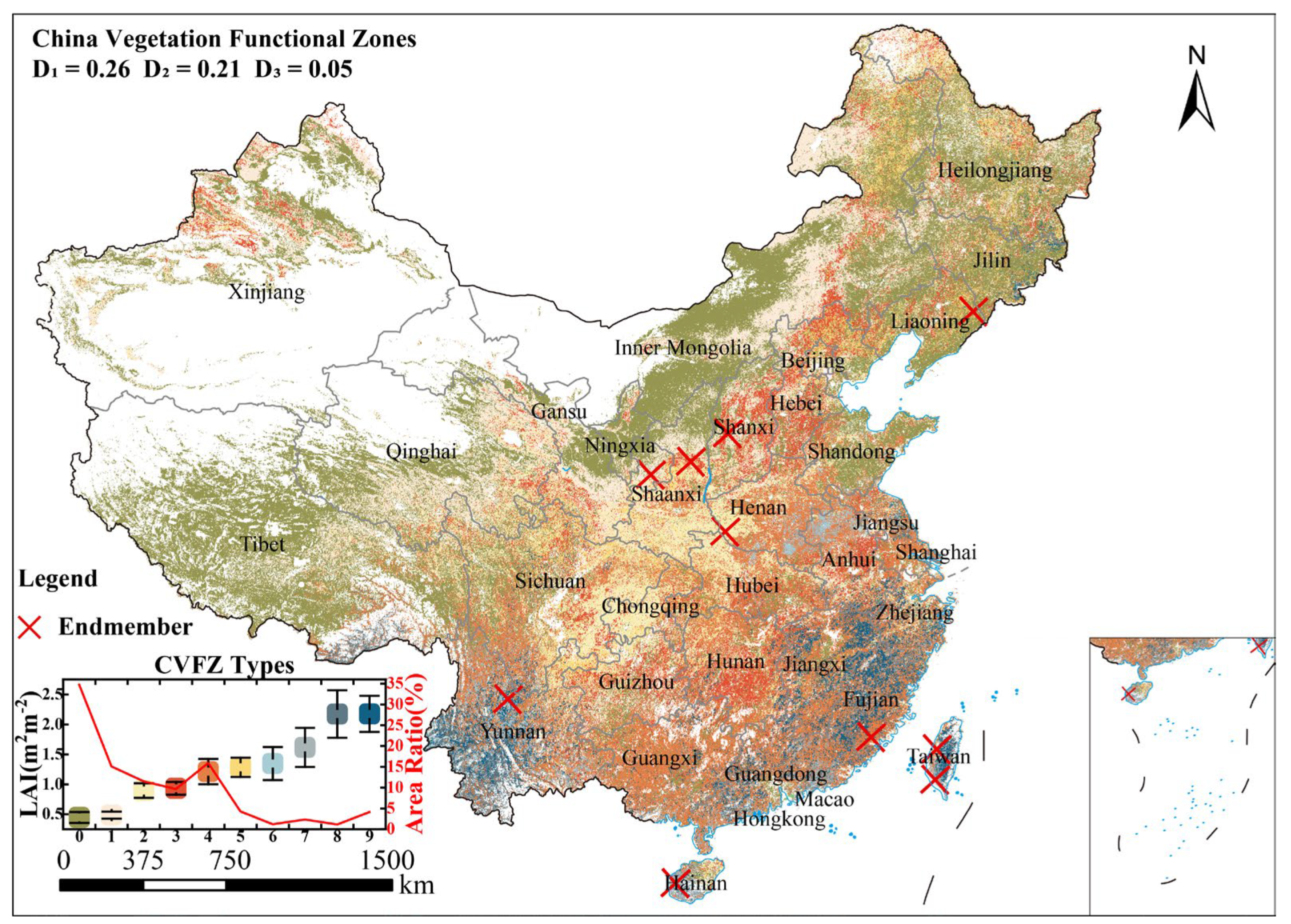
The map of the classification results is displayed in Figure 3, and the 10 vegetation zones are named from 0 to 9 in order of increasing average LAI. The LAI mean values for the 10 zones were 0.45, 0.49, 0.90, 0.93, 1.21, 1.28, 1.35, 1.62, 2.17, and 2.18, respectively. The overall distribution of the zones showed a certain northeast-southwest pattern. Among them, 0 types accounted for 34.7%, 4 types accounted for 15.9%, 1 types accounted for 15.1%, and 2 types accounted for 11.5%.

3.2. Enhanced Discrimination Compared to Land Cover Datasets

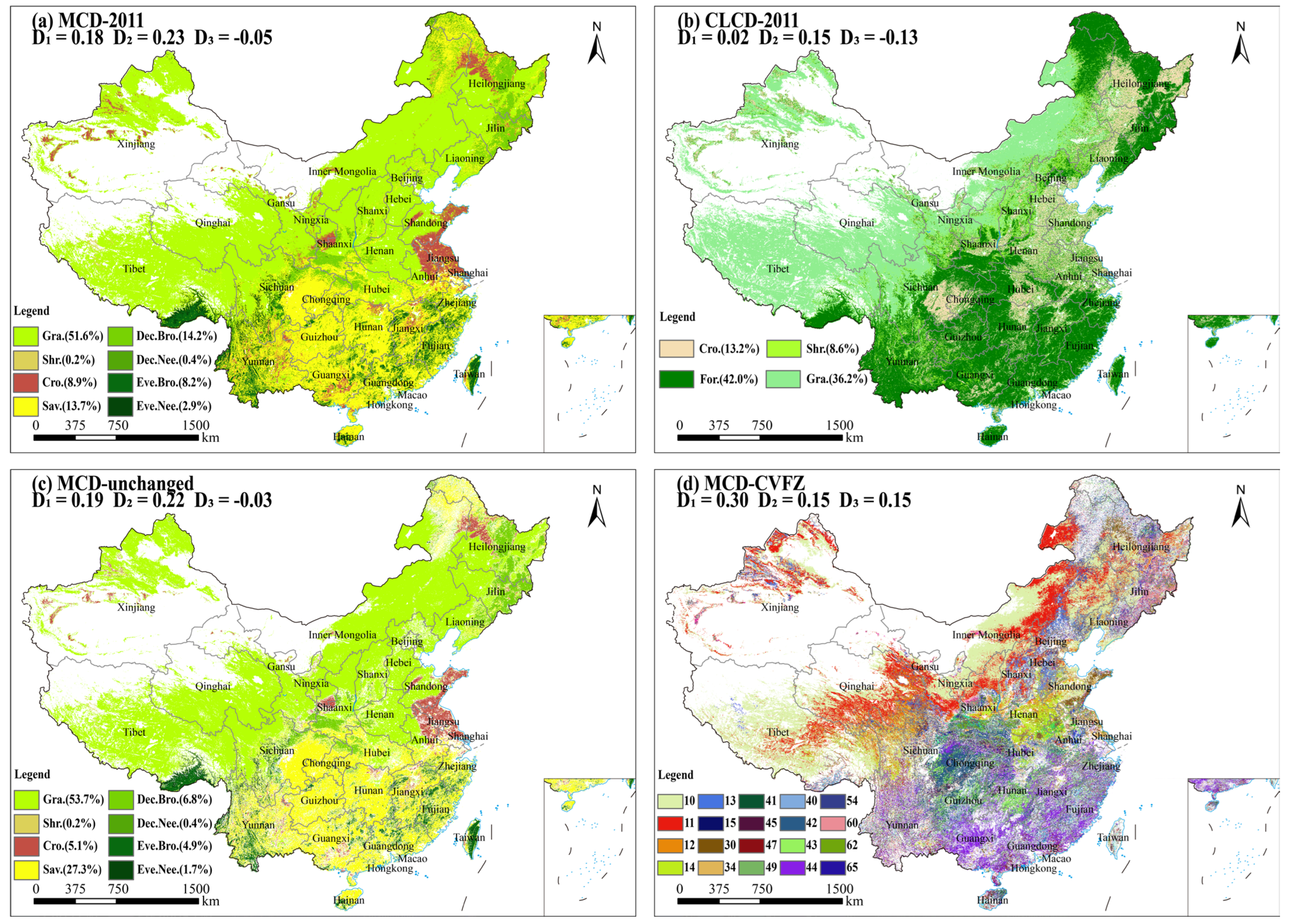
Figure 4 depicts the results of cross-validation for MCD-CVFZ and several land cover products. The validation results of CVFZ in Figure 3 (D3 = 0.05) are better than MCD-2011 (D3 = −0.05), CLCD-2011 (D3 = −0.13), and MCD-unchanged (D3 = −0.03), highlighting the necessity of differentiating vegetation function and emphasizing the effectiveness of CVFZ in achieving this goal. The D1 of MCD-2011 and MCD-unchanged is slightly smaller than D2, and, correspondingly, D3 is slightly below zero. In other words, the closer D1 and D2 are, the smaller the difference in LAI multi-temporal spectra between two vegetation pixels from the same or different types tend to be and the smaller the ability to distinguish vegetation functions. The evaluation results of MCD-unchanged were slightly better than MCD-2011 (Figure 4a,c), indicating the need to use pixels with an unchanged vegetation type for cutting. The proportion of savannas in MCD-unchanged increased from 13.7% to 27.3% compared to that of MCD-2011, while forested areas decreased from 25.7% to 13.8%, and broadleaf crops decreased from 8.9% to 5.1%, indicating recent degradation of forests and loss of farmland in China during the past few years, which may be related to the country’s large-scale urbanization process. The value of D3 in CLCD-2011 is only −0.13 (Figure 4b), which may be related to the fact that vegetation types are only divided into four regions or that the data source is not consistent with the LAI dataset. MCD-CVFZ obtained the best validation results with D1 = 0.30, D2 = 0.15, and D3 = 0.15, which may be due to the distinction between vegetation function and vegetation type, simultaneously (Figure 4d).

3.3. Performance of CVFZ on Distinguishing LAI Mean Value and LAI Time Series

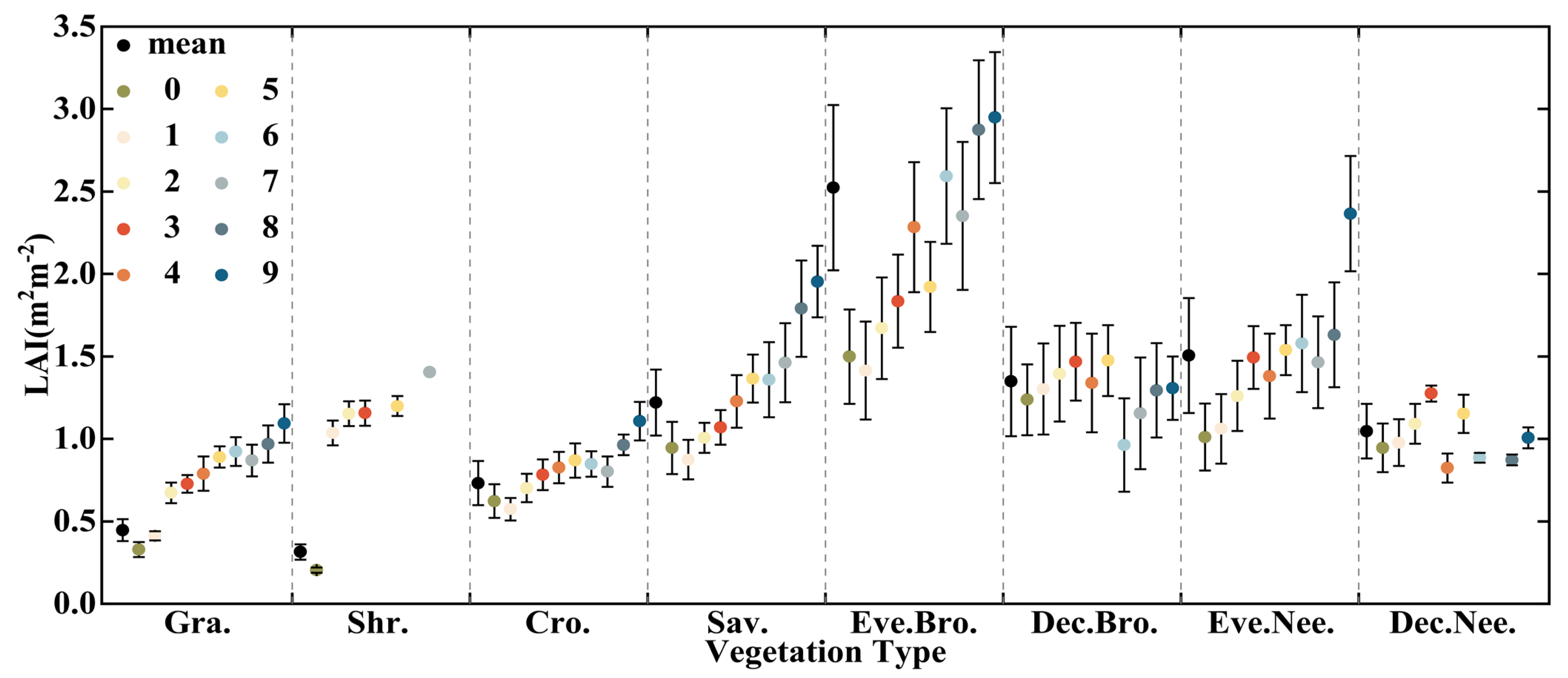
In Figure 5, the performance of CVFZ in distinguishing between the mean and standard deviation of LAI is presented. CVFZ distinguishes vegetation functions from the LAI mean in different vegetation types, and an increasing trend is observed in the mean and standard deviation of LAI of each zone from 0 type to 9 type. Fluctuations in the LAI mean are observed in deciduous broadleaf forests and deciduous needleleaf forests, which may be attributed to the small area of these two vegetation covers.
Figure 6 demonstrates the performance of CVFZ in distinguishing LAI time series. The results show that CVFZ effectively distinguishes vegetation functions from the LAI time series as well. The LAI time series of a higher type in CVFZ are generally above that of a lower type. Moreover, the LAI sequences of shrublands with different functions are distinctly separated (Figure 6b), with the 20-type LAI time series fluctuating in the range of 0.1–0.4 m2m−2, while the 25-type LAI time series fluctuates in the range of 0.2–4.1 m2m−2.

3.4. Analysis of Annual and Intra-Annual LAI Fluctuations in Different Vegetation Types

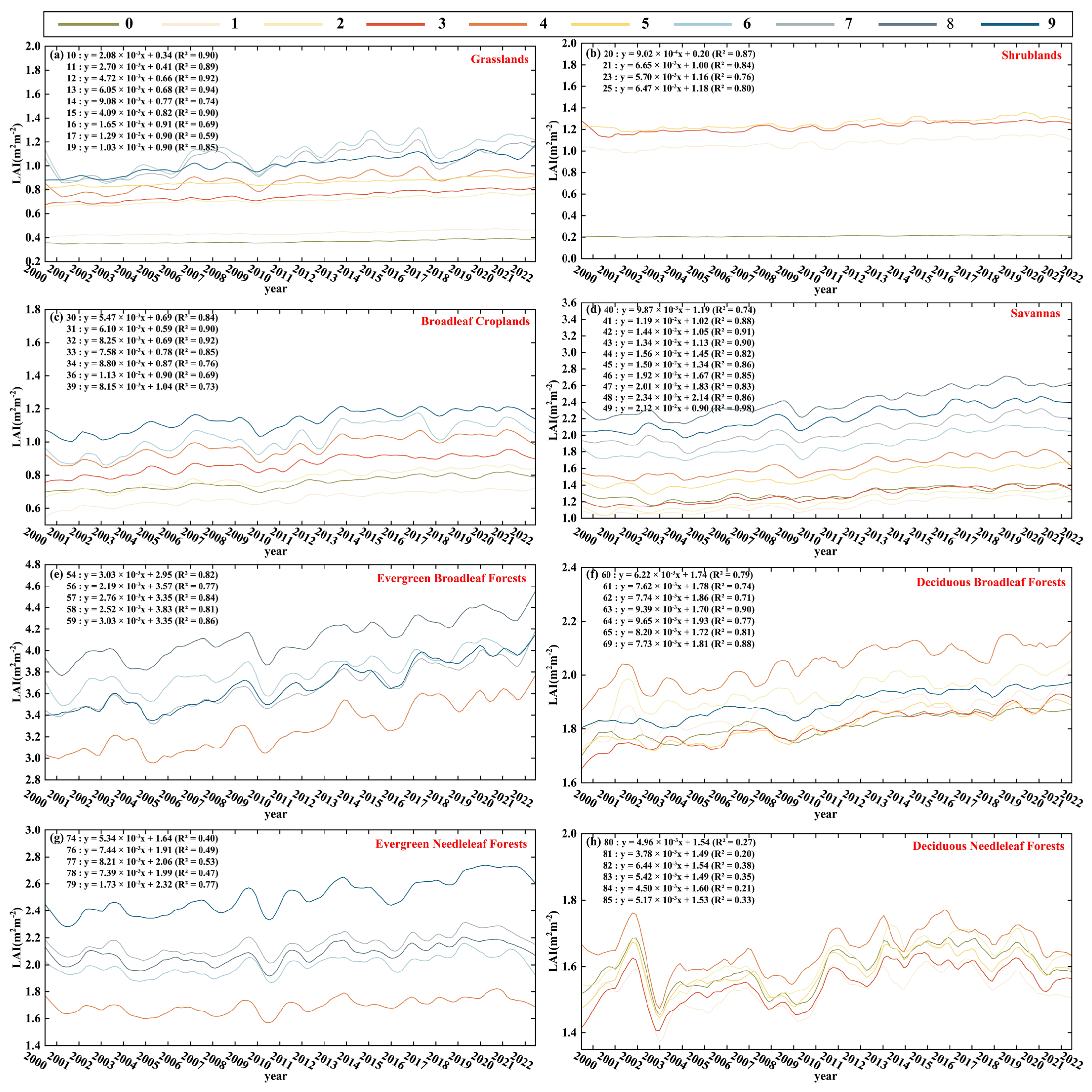
According to the results presented in Figure 7 and Figure 8, the STL method is more effective in reflecting vegetation function specificity. The goodness of fit in Figure 7 indicates a high overall goodness of fit, except for two types of needleleaf forest vegetation. For the same vegetation, the greening speed generally increases and then decreases with an increase in the corresponding CVFZ vegetation category, and the slope reaches its peak at around 4–6 types, while the starting value of annual fluctuations shows an increasing trend of volatility. The greening speed of grasslands varies by up to 8 times from 2.08 × 10⁻³ m2m−2yr−1 to 1.65 × 10⁻² m2m−2yr−1 (Figure 7a). The starting value of the annual fluctuation of LAI in shrublands differs by up to 6 from 0.20 m2m−2 to 1.18 m2m−2 (Figure 7b).
Among the different vegetation, the initiation of LAI annual fluctuation was the largest in evergreen broadleaf forests and the smallest in grasslands, at 2.95 m2m−2 and 0.34 m2m−2, respectively (Figure 7e). On average, all vegetation in subregions of MCD-CVFZ showed varying degrees of greening. Savanna subregions had the fastest greening speed between 9.87 × 10⁻³ m2m−2yr−1 and 2.34 × 10⁻² m2m−2yr−1, while shrubland subregions had the slowest greening speed between 9.02 × 10⁻⁴ m2m−2yr−1 and 6.65 × 10⁻² m2m−2yr−1.
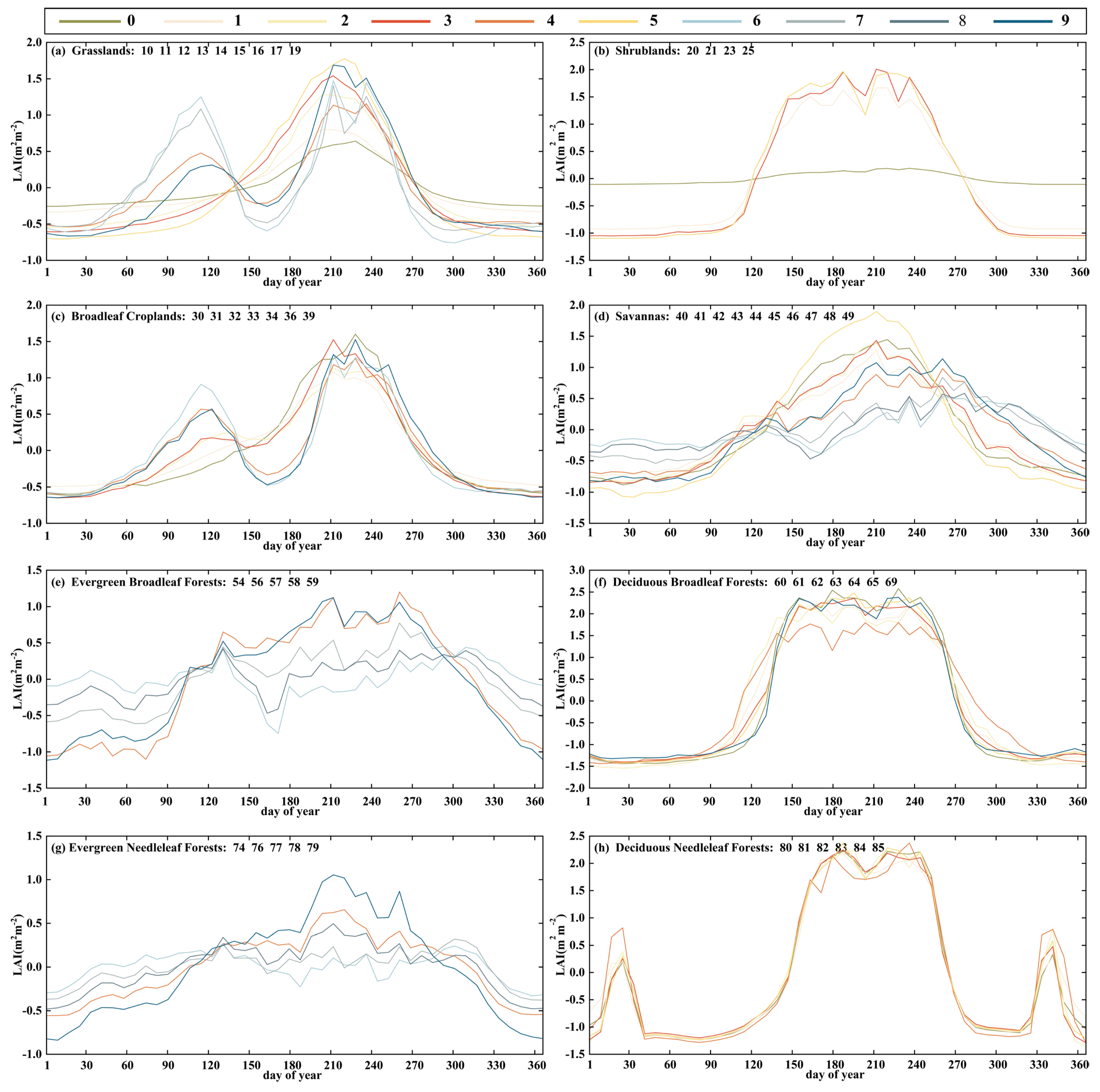
Figure 8 illustrates that for the same type of vegetation, the CVFZ is capable of distinguishing growth characteristics and phenological cycles of vegetation. A higher type of CVFZ generally corresponds to a lagging phenological cycle and sometimes even an increase in the phenological cycle. For instance, the vegetation types 10, 11, 12, 13, and 15 in Figure 8a represent grasslands with a phenological cycle that reaches its peak greenness on Days 200 to 230, while 14, 16, 17, and 18 indicate grasslands with two phenological cycles, and their greenness reaches a second peak on Days 210 to 240. Figure 8b shows shrublands of vegetation type 20 with a not-so-obvious phenological cycle, and 21, 23, and 25 represent shrublands with one phenological cycle. The same trend is observed in broadleaf crops, where the vegetation types 30, 31, and 32 indicate crops with a phenological cycle, whose greenness peaks on Days 210 to 225, while 34, 36, and 39 represent crops with two phenological cycles, and their greenness reaches a second peak at around Day 225 (Figure 8c).
Regarding the main phenological cycle, deciduous broadleaf forests have the earliest peak greenness, which occurs at approximately Days 150 to 250 (Figure 8f), which is close to that of shrublands with a phenological cycle (Figure 8b), while broadleaf crops have the latest peak greenness, which occurs at approximately Days 210 to 250 (Figure 8c). Peak greenness in deciduous needleleaf forests occurs from Days 190 to 250, and the duration period of greenness peaks is shorter and later than that of deciduous broadleaf forests (Figure 8h). The intra-annual greenness fluctuations range most widely in deciduous broadleaf forests, between −1.5 m2m−2 and 2.5 m2m−2, while in evergreen needleleaf forests, they are the smallest, ranging between −0.8 m2m−2 and 1.0 m2m−2 (Figure 8g). For evergreen broadleaf forests, the intra-annual greenness fluctuations range between −1.1 m2m−2 and 1.2 m2m−2, but there is no obvious peak greenness (Figure 8e).

4. Discussion

4.1. Potential Advantage of the Use of CVFZ in Vegetation Analysis and Policymaking

Furthermore, in addition to distinguishing vegetation functions, the screening of highly representative and high-quality vegetation pixels could be a potential advantage of CVFZ in vegetation analysis. As illustrated in Figure 9 with MCD-2011, after being filtered by CVFZ, 81.3% of pixels were retained, and the D2 of different zones decreased, except for the evergreen broadleaf forest. The average D2 value decreased from 0.2309 to 0.2247. Notably, the LAI average of shrublands decreased from 0.53 to 0.32 in 2011, which is closer to Sang et al.’s research conclusions [79]. This demonstrates that the remaining pixels of MCD-2011 exhibit higher similarity, which indicates potentially higher classification accuracy. This is because the VCA–MLC process does not require any land cover products as prior knowledge, thereby avoiding issues such as the misclassification of vegetation pixels in land cover products to some extent.
Furthermore, CVFZ can also be used in conjunction with other land cover maps to further analyze vegetation for different functions. In this study, MCD12Q1 was used as an example because the use of MODIS products in classification and cutting can better ensure the consistency of results [62]. Additionally, because vegetation functions are distinguished at pixel scale, CVFZ can be utilized to analyze the differences in vegetation in a specific area, and it has significance for scientific analysis in climatology, ecology, and vegetation.
As a derivative product of the hyperspectral image classification algorithm in multi-temporal image classification, CVFZ has several areas that could be improved. For instance, the process of endmember extraction could incorporate more LAI time phases, and the screening of LAI endmembers could introduce other prior knowledge. Additionally, the MLC process could be combined with machine learning methods [80,81,82].
Ecosystem services bridge the gap between policymaking and actual benefits by linking ecosystem characteristics as intermediate services and to human well-being as the ultimate service [83]. Our research helps map ecosystem services and establish indicators of the monitored ecosystems and final services, thus effectively mitigating the negative causality between local ecological change and economic growth [84]. In addition, where aspects such as agriculture of crop, livestock, and silvicultural production and environmental legislation for sustainability conflict [85], CVFZ can serve as a direct basis for conflict resolution. For example, lower zoning areas focus on agricultural development while higher zoning areas focus on environmental protection. The variation in vegetation exposure reflected by zoning types also provides new perspectives for thinking about vegetation type, quantity, and different spatial scales of study [86].

4.2. Spatial Variability of Vegetation Dynamics Revealed by CVFZ

Figure 10 depicts the spatial variability in vegetation dynamics captured by CVFZ, which reveals a large void in the central Sichuan region. The corresponding blank region in the global topographic map aligns well with the Chengdu Plain, which is predominantly an urban area [87]. The blank region’s southwestern side corresponds to the Hengduan Mountains, where the CVFZ types are mainly 0 and 2, while the blank area’s northeastern side corresponds to the Sichuan Basin, where the CVFZ types are primarily 3, 4, and 5.
The vegetation types in the regions differ significantly based on MCD12Q1. Evergreen broadleaf forests cover only a small portion of the Chengdu Plain, while the Hengduan Mountains feature grasslands (represented by MCD-CVFZ types 10 and 12) with a greening speed of 2.08 × 10⁻³ m2m−2yr−1 to 4.72 × 10⁻³ m2m−2yr−1, respectively. In contrast, the Sichuan Basin is predominantly savannas (represented by MCD-CVFZ types 43, 44, and 45) with a greening speed of 1.34 × 10⁻² m2m−2yr−1 to 1.56 × 10⁻² m2m−2yr−1, which is nearly six times that of the Hengduan Mountains.
Although the five vegetation types share the same phenological cycle of 1, the LAI intra-annual fluctuation of the two grassland vegetation types smoothly rises before decreasing between −0.3 m2m−2 and 1.1 m2m−2, peaking between Days 200 and 230. In contrast, the three savanna vegetation types have a volatility between −1.1 m2m−2 and 1.9 m2m−2, with peaks around Day 210. The significant variability in potential vegetation dynamics between geographically similar regions illustrates the value of CVFZ land use management in China.

4.3. Drivers of Vegetation Dynamics as Jointly Explained with Other Studies

The growth of vegetation is influenced by various drivers, such as climate change and human activities [88]. Temperature is a major contributor to the spatial and temporal changes in vegetation growth dynamics nationwide, and human factors such as afforestation, urbanization, and agricultural practices also affect vegetation growth in certain regions [89,90]. This is demonstrated by the dramatic change in the proportion of vegetation types found in this study (Figure 4a,d). Zhang et al. [91] found that the mean and standard deviation of China LAI exhibited a gradient from northwest to southeast, which was closely related to the temperature change pattern. This pattern is consistent with the observation that the CVFZ zone displays a northeast-southwest distribution pattern (Figure 3). Moreover, the trends in vegetation dynamics show significant regional and seasonal heterogeneity.
Southern China is more affected by temperature, while most of the grasslands in northern China are more influenced by precipitation. According to Piao et al. [92] and Munier et al. [93], greening has been observed in most parts of China during this century, while Inner Mongolia, dominated by winter crops and needleleaf forests, has experienced reduced precipitation and consequent browning of vegetation due to frequent droughts [82]. Additionally, Maimaitiyiming et al. [94] found that changes in precipitation in high-temperature and water-scarce areas, such as the Aksu region of northwest China, trigger the urban heat island effect by affecting urban green spaces. Tang et al. [95] studied the vegetation greening in northern Xinjiang and browning in northeastern Inner Mongolia, and further revealed the significant impact of climate change on vegetation dynamics from a phenological perspective.
Li et al. [96] and Huang et al. [97] have observed a trend in vegetation greening at the average level on the Tibetan Plateau over the course of this century. This is mainly due to increased precipitation, permafrost degradation, and a decrease in overgrazing. The study also found significant changes in vegetation dynamics in most ecosystem areas around 2007–2010. In this study, a significant decline in the annual fluctuation sequence of LAI was found in most vegetation around 2010, with a decline as high as 0.2 m2m−2 in evergreen broadleaf forests (Figure 9). Song et al. [98] reported a browning trend in most vegetation dominated by alpine meadows in the high-altitude areas of Cocoxili. This study further reported that the grasslands of the Qinghai–Tibet Plateau, dominated by types 10 and 11 (Figure 4d), had a weak greening trend of 2.08 × 10⁻³ m2m−2yr−1 to 2.70 × 10⁻³ m2m−2yr−1 (Figure 7a).
Regarding urban areas, the impact of human activities on vegetation dynamics is heterogeneous, with greening occurring in some areas. Jiang et al. [99] and Huang et al. [100] studied vegetation loss in the Beijing area from 2000 to 2015, which occurred mainly in the area between the fourth and sixth ring roads, while vegetation restoration and increase mainly occurred in the Beijing Plain. This is due to economic development and local ecological restoration projects. Tong et al. [101] reported that ecological restoration projects have led to the greening of vegetation in much of southwest China between 2001 and 2011.
Seasonally, changes in spring and autumn are mainly temperature-driven, while in summer, precipitation in parts of northern China is slightly more predominant. Xu et al. [55] and Liu et al. [102] have found a nationwide trend of an increased vegetation index driven by rising average temperatures in spring and autumn, while precipitation has been in decline in summer since the 1982 limits vegetation growth in parts of northern China, such as northeastern Inner Mongolia.

5. Conclusions

This study presents an innovative approach that divides China’s vegetation area into 10 zones, forming a novel product termed China Vegetation Functional Zones (CVFZ). The primary findings of this study are summarized below:
  • Firstly, CVFZ outperforms MCD12Q1 and CLCD, exhibiting superior performance in distinguishing vegetation with varying functions. Even in smaller zones, CVFZ can also well distinguish vegetation with different functions from the angle of LAI mean or the LAI time series. Although this study does not cover further measured tests, it indicates that the use of the VCA–MLC algorithm provides some taxonomic value in vegetation studies. The resulting CVFZ derivative product offers valuable information for climate and ecological monitoring and management.
  • Secondly, the speed of greening of vegetation ranges from 9.02 × 10⁻⁴ m2m−2yr−1 in shrubland subregions to 2.34 × 10⁻² m2m−2yr−1 in savanna subregions. In relative terms, the average greening speed of forests is moderate, and savannas tend to have the fastest average greening speed. The average greening speed of grasslands and crops with different functions varies widely. In contrast, the average greening speed of shrublands is the smallest.
  • Thirdly, as the location of CVFZ shifts to a higher type within the same vegetation, the greening speed generally increases and then decreases, with the slope peaking around types 4–6, and the phenological cycle generally lags but tends to increase; for example, CVFZ-detected grasslands with one or two phenological cycles, broadleaf crops with one or two phenological cycles, and shrublands with one or not-so-obvious phenological cycles.

Author Contributions

T.X.: formal analysis and writing—original draft preparation. K.Y. (Kai Yan): conceptualization, methodology, writing—review and editing, funding acquisition, supervision, and project administration. Y.H.: validation and software. S.G.: visualization. K.Y. (Kai Yang): formal analysis. J.W.: investigation. J.L.: editing. Z.L.: resources. All authors have read and agreed to the published version of the manuscript.

Funding

This work was supported by the National Natural Science Foundation of China Major Program (42192580) and the National Natural Science Foundation of China (42271356).

Data Availability Statement

The data used in the study is publicly available.

Acknowledgments

We thank the MODIS LAI & FPAR team for all their help and the team of Yang Jie and Huang Xin of Wuhan University for support with the CLCD dataset. We also appreciate the fruitful suggestions from the anonymous reviewers which made the work better.

Conflicts of Interest

The authors declare no conflict of interest.

References

  1. Zeng, J.; Zhang, Q.; Zhang, Y.; Yue, P.; Yang, Z.S.; Wang, S.; Zhang, L.; Li, H.Y. Enhanced Impact of Vegetation on Evapotranspiration in the Northern Drought-Prone Belt of China. Remote Sens. 2023, 15, 221. [Google Scholar] [CrossRef]
  2. Liu, Y.B.; Xiao, J.F.; Ju, W.M.; Zhu, G.L.; Wu, X.C.; Fan, W.L.; Li, D.Q.; Zhou, Y.L. Satellite-derived LAI products exhibit large discrepancies and can lead to substantial uncertainty in simulated carbon and water fluxes. Remote Sens. Environ. 2018, 206, 174–188. [Google Scholar] [CrossRef]
  3. Xiao, J.Y.; Xie, B.G.; Zhou, K.C.; Li, J.N.; Xie, J.; Liang, C. Contributions of Climate Change, Vegetation Growth, and Elevated Atmospheric CO2 Concentration to Variation in Water Use Efficiency in Subtropical China. Remote Sens. 2022, 14, 4296. [Google Scholar] [CrossRef]
  4. Claverie, M.; Matthews, J.L.; Vermote, E.F.; Justice, C.O. A 30+Year AVHRR LAI and FAPAR Climate Data Record: Algorithm Description and Validation. Remote Sens. 2016, 8, 263. [Google Scholar] [CrossRef] [Green Version]
  5. Bo, Y.; Li, X.K.; Liu, K.; Wang, S.D.; Zhang, H.Y.; Gao, X.J.; Zhang, X.Y. Three Decades of Gross Primary Production (GPP) in China: Variations, Trends, Attributions, and Prediction Inferred from Multiple Datasets and Time Series Modeling. Remote Sens. 2022, 14, 2564. [Google Scholar] [CrossRef]
  6. Houborg, R.; Soegaard, H.; Boegh, E. Combining vegetation index and model inversion methods for the extraction of key vegetation biophysical parameters using Terra and Aqua MODIS reflectance data. Remote Sens. Environ. 2007, 106, 39–58. [Google Scholar] [CrossRef]
  7. Yan, H.; Wang, S.Q.; Billesbach, D.; Oechel, W.; Zhang, J.H.; Meyers, T.; Martin, T.A.; Matamala, R.; Baldocchi, D.; Bohrer, G.; et al. Global estimation of evapotranspiration using a leaf area index-based surface energy and water balance model. Remote Sens. Environ. 2012, 124, 581–595. [Google Scholar] [CrossRef] [Green Version]
  8. Kern, A.; Barcza, Z.; Hollos, R.; Birinyi, E.; Marjanovic, H. Critical Climate Periods Explain a Large Fraction of the Observed Variability in Vegetation State. Remote Sens. 2022, 14, 5621. [Google Scholar] [CrossRef]
  9. Dai, X.A.; Fan, W.J.; Shan, Y.F.; Gao, Y.; Liu, C.; Nie, R.H.; Zhang, D.H.; Li, W.L.; Zhang, L.F.; Sun, X.J.; et al. LAI-Based Phenological Changes and Climate Sensitivity Analysis in the Three-River Headwaters Region. Remote Sens. 2022, 14, 3748. [Google Scholar] [CrossRef]
  10. Vremec, M.; Forstner, V.; Herndl, M.; Collenteur, R.; Schaumberger, A.; Birk, S. Sensitivity of evapotranspiration and seepage to elevated atmospheric CO2 from lysimeter experiments in a montane grassland. J. Hydrol. 2023, 617, 128875. [Google Scholar] [CrossRef]
  11. Cook, B.; Zeng, N.; Yoon, J.H. Will Amazonia Dry Out? Magnitude and Causes of Change from IPCC Climate Model Projections. Earth Interact. 2012, 16, 1–27. [Google Scholar] [CrossRef] [Green Version]
  12. Lawal, S.; Lennard, C.; Jack, C.; Wolski, P.; Hewitson, B.; Abiodun, B. The observed and model-simulated response of southern African vegetation to drought. Agric. For. Meteorol. 2019, 279, 107698. [Google Scholar] [CrossRef]
  13. Zhang, W.; Wang, L.C.; Xiang, F.F.; Qin, W.M.; Jiang, W.X. Vegetation dynamics and the relations with climate change at multiple time scales in the Yangtze River and Yellow River Basin, China. Ecol. Indic. 2020, 110, 105892. [Google Scholar] [CrossRef]
  14. Jiao, W.Z.; Wang, L.X.; McCabe, M.F. Multi-sensor remote sensing for drought characterization: Current status, opportunities and a roadmap for the future. Remote Sens. Environ. 2021, 256, 112313. [Google Scholar] [CrossRef]
  15. Holm, J.A.; Chambers, J.Q.; Collins, W.D.; Higuchi, N. Forest response to increased disturbance in the central Amazon and comparison to western Amazonian forests. Biogeosciences 2014, 11, 5773–5794. [Google Scholar] [CrossRef] [Green Version]
  16. Yang, Y.J.; Huang, W.; Xie, T.T.; Li, C.X.; Deng, Y.J.; Chen, J.; Liu, Y.; Ma, S. Elevation Gradients Limit the Antiphase Trend in Vegetation and Its Climate Response in Arid Central Asia. Remote Sens. 2022, 14, 5922. [Google Scholar] [CrossRef]
  17. Qiu, L.J.; Liu, X.D. Sensitivity analysis of modelled responses of vegetation dynamics on the Tibetan Plateau to doubled CO2 and associated climate change. Theor. Appl. Climatol. 2016, 124, 229–239. [Google Scholar] [CrossRef]
  18. Piao, S.L.; Ciais, P.; Huang, Y.; Shen, Z.H.; Peng, S.S.; Li, J.S.; Zhou, L.P.; Liu, H.Y.; Ma, Y.C.; Ding, Y.H.; et al. The impacts of climate change on water resources and agriculture in China. Nature 2010, 467, 43–51. [Google Scholar] [CrossRef]
  19. Zhang, J.; Wu, H.Q.; Zhang, Z.; Zhang, L.L.; Luo, Y.C.; Han, J.C.; Tao, F.L. Asian Rice Calendar Dynamics Detected by Remote Sensing and Their Climate Drivers. Remote Sens. 2022, 14, 4189. [Google Scholar] [CrossRef]
  20. Luo, H.; Bie, X.J.; Yi, G.H.; Zhou, X.B.; Zhang, T.B.; Li, J.J.; Lai, P.Q. Dominant Impacting Factors on Water-Use Efficiency Variation in Inner Mongolia from 2001 to 2018: Vegetation or Climate? Remote Sens. 2022, 14, 4541. [Google Scholar] [CrossRef]
  21. Yu, Z.X.; Wang, T.Y.; Wang, P.; Yu, J.J. The Spatiotemporal Response of Vegetation Changes to Precipitation and Soil Moisture in Drylands in the North Temperate Mid-Latitudes. Remote Sens. 2022, 14, 3511. [Google Scholar] [CrossRef]
  22. Wang, M.M.; Zhao, J.; Wang, S.Q.; Chen, B. Regional Contributions and Climate Attributions to Interannual Variation of Global Net Ecosystems Production by an ECOSYSTEM Processed Model Driven by Remote Sensing Data over the Past 35 Years. Remote Sens. 2022, 14, 3208. [Google Scholar] [CrossRef]
  23. Forzieri, G.; Alkama, R.; Miralles, D.G.; Cescatti, A. Satellites reveal contrasting responses of regional climate to the widespread greening of Earth. Science 2017, 356, 1140–1144. [Google Scholar] [CrossRef] [PubMed] [Green Version]
  24. Zeng, Z.Z.; Piao, S.L.; Li, L.Z.X.; Zhou, L.M.; Ciais, P.; Wang, T.; Li, Y.; Lian, X.; Wood, E.F.; Friedlingstein, P.; et al. Climate mitigation from vegetation biophysical feedbacks during the past three decades. Nat. Clim. Chang. 2017, 7, 432–436. [Google Scholar] [CrossRef]
  25. Zhu, Z.C.; Piao, S.L.; Myneni, R.B.; Huang, M.T.; Zeng, Z.Z.; Canadell, J.G.; Ciais, P.; Sitch, S.; Friedlingstein, P.; Arneth, A.; et al. Greening of the Earth and its drivers. Nat. Clim. Chang. 2016, 6, 791–795. [Google Scholar] [CrossRef]
  26. Zhang, Y.L.; Song, C.H.; Band, L.E.; Sun, G.; Li, J.X. Reanalysis of global terrestrial vegetation trends from MODIS products: Browning or greening? Remote Sens. Environ. 2017, 191, 145–155. [Google Scholar] [CrossRef] [Green Version]
  27. Zhou, Y.Q.; Li, Y.M.; Li, W.; Li, F.; Xin, Q.C. Ecological Responses to Climate Change and Human Activities in the Arid and Semi-Arid Regions of Xinjiang in China. Remote Sens. 2022, 14, 3911. [Google Scholar] [CrossRef]
  28. Caracciolo, D.; Istanbulluoglu, E.; Noto, L.V. An Ecohydrological Cellular Automata Model Investigation of Juniper Tree Encroachment in a Western North American Landscape. Ecosystems 2017, 20, 1104–1123. [Google Scholar] [CrossRef]
  29. Andela, N.; Liu, Y.Y.; van Dijk, A.; de Jeu, R.A.M.; McVicar, T.R. Global changes in dryland vegetation dynamics (1988–2008) assessed by satellite remote sensing: Comparing a new passive microwave vegetation density record with reflective greenness data. Biogeosciences 2013, 10, 6657–6676. [Google Scholar] [CrossRef] [Green Version]
  30. Li, X.J.; Qu, Y. Evaluation of Vegetation Responses to Climatic Factors and Global Vegetation Trends using GLASS LAI from 1982 to 2010. Can. J. Remote Sens. 2018, 44, 357–372. [Google Scholar] [CrossRef]
  31. Curasi, S.R.; Parker, T.C.; Rocha, A.V.; Moody, M.L.; Tang, J.W.; Fetcher, N. Differential responses of ecotypes to climate in a ubiquitous Arctic sedge: Implications for future ecosystem C cycling. New Phytol. 2019, 223, 180–192. [Google Scholar] [CrossRef] [PubMed] [Green Version]
  32. McManus, K.M.; Morton, D.C.; Masek, J.G.; Wang, D.D.; Sexton, J.O.; Nagol, J.R.; Ropars, P.; Boudreau, S. Satellite-based evidence for shrub and graminoid tundra expansion in northern Quebec from 1986 to 2010. Glob. Chang. Biol. 2012, 18, 2313–2323. [Google Scholar] [CrossRef] [Green Version]
  33. Law, B.E.; Falge, E.; Gu, L.; Baldocchi, D.D.; Bakwin, P.; Berbigier, P.; Davis, K.; Dolman, A.J.; Falk, M.; Fuentes, J.D.; et al. Environmental controls over carbon dioxide and water vapor exchange of terrestrial vegetation. Agric. For. Meteorol. 2002, 113, 97–120. [Google Scholar] [CrossRef] [Green Version]
  34. Miller, P.A.; Smith, B. Modelling Tundra Vegetation Response to Recent Arctic Warming. Ambio 2012, 41, 281–291. [Google Scholar] [CrossRef] [Green Version]
  35. Kim, K.; Wang, M.C.; Ranjitkar, S.; Liu, S.H.; Xu, J.C.; Zomer, R.J. Using leaf area index (LAI) to assess vegetation response to drought in Yunnan province of China. J. Mt. Sci. 2017, 14, 1863–1872. [Google Scholar] [CrossRef]
  36. Zhang, X.M.; He, G.J.; Zhang, Z.M.; Peng, Y.; Long, T.F. Spectral-spatial multi-feature classification of remote sensing big data based on a random forest classifier for land cover mapping. Clust. Comput.—J. Netw. Softw. Tools Appl. 2017, 20, 2311–2321. [Google Scholar] [CrossRef]
  37. Hayes, M.M.; Miller, S.N.; Murphy, M.A. High- resolution landcover classification using Random Forest. Remote Sens. Lett. 2014, 5, 112–121. [Google Scholar] [CrossRef]
  38. Liu, X.; Hu, G.; Chen, Y.; Li, X.; Xu, X.; Li, S.; Pei, F.; Wang, S. High-resolution multi-temporal mapping of global urban land using Landsat images based on the Google Earth Engine Platform. Remote Sens. Environ. 2018, 209, 227–239. [Google Scholar] [CrossRef]
  39. Ma, L.; Liu, Y.; Zhang, X.L.; Ye, Y.X.; Yin, G.F.; Johnson, B.A. Deep learning in remote sensing applications: A meta-analysis and review. Isprs J. Photogramm. Remote Sens. 2019, 152, 166–177. [Google Scholar] [CrossRef]
  40. Torabzadeh, H.; Morsdorf, F.; Schaepman, M.E. Fusion of imaging spectroscopy and airborne laser scanning data for characterization of forest ecosystems—A review. Isprs J. Photogramm. Remote Sens. 2014, 97, 25–35. [Google Scholar] [CrossRef]
  41. Yang, Y.; Xiao, P.; Feng, X.; Li, H. Accuracy assessment of seven global land cover datasets over China. ISPRS J. Photogramm. Remote Sens. 2017, 125, 156–173. [Google Scholar] [CrossRef]
  42. Su, Y.; Guo, Q.; Xue, B.; Hu, T.; Alvarez, O.; Tao, S.; Fang, J. Spatial distribution of forest aboveground biomass in China: Estimation through combination of spaceborne lidar, optical imagery, and forest inventory data. Remote Sens. Environ. 2016, 173, 187–199. [Google Scholar] [CrossRef] [Green Version]
  43. Hou, P.; Chen, Y.; Zhai, J.; Hou, J.; Yang, M.; Jin, D.; Zhu, H.; Gao, H.; Wan, H.; Fu, Z. Natural Ecological Background of Terrestrial Vegetation in China: Identification Methods and Spatial Differentiation Characteristics. Sens. Mater. 2021, 33, 4659–4680. [Google Scholar] [CrossRef]
  44. Seidl, M.; Saifane, M. A green intensity index to better assess the multiple functions of urban vegetation with an application to Paris metropolitan area. Environ. Dev. Sustain. 2021, 23, 15204–15224. [Google Scholar] [CrossRef]
  45. Houborg, R.; Fisher, J.B.; Skidmore, A.K. Advances in remote sensing of vegetation function and traits. Int. J. Appl. Earth Obs. Geoinf. 2015, 43, 1–6. [Google Scholar] [CrossRef] [Green Version]
  46. Pu, J.B.; Yan, K.; Zhou, G.H.; Lei, Y.Q.; Zhu, Y.X.; Guo, D.H.; Li, H.L.; Xu, L.L.; Knyazikhin, Y.; Myneni, R.B. Evaluation of the MODIS LAI/FPAR Algorithm Based on 3D-RTM Simulations: A Case Study of Grassland. Remote Sens. 2020, 12, 3391. [Google Scholar] [CrossRef]
  47. Cui, L.; Wang, L.; Singh, R.P.; Lai, Z.; Jiang, L.; Yao, R. Association analysis between spatiotemporal variation of vegetation greenness and precipitation/temperature in the Yangtze River Basin (China). Environ. Sci. Pollut. Res. 2018, 25, 21867–21878. [Google Scholar] [CrossRef]
  48. Li, X.L.; Lu, H.; Yu, L.; Yang, K. Comparison of the Spatial Characteristics of Four Remotely Sensed Leaf Area Index Products over China: Direct Validation and Relative Uncertainties. Remote Sens. 2018, 10, 148. [Google Scholar] [CrossRef] [Green Version]
  49. Peng, Z.; Li, Y.; Yu, W.; Xing, Y.; Feng, A.; Du, S. Research on the Applicability of Remote Sensing Precipitation Products in Different Climatic Regions of China. J. Geo-Inf. Sci. 2021, 23, 1296–1311. [Google Scholar]
  50. Wei, F.L.; Wang, S.; Fu, B.J.; Pan, N.Q.; Feng, X.M.; Zhao, W.W.; Wang, C. Vegetation dynamic trends and the main drivers detected using the ensemble empirical mode decomposition method in East Africa. Land Degrad. Dev. 2018, 29, 2542–2553. [Google Scholar] [CrossRef]
  51. Chen, Z.; Chen, Y.; Bai, L.; Xu, J. Multiscale evolution of surface air temperature in the arid region of Northwest China and its linkages to ocean oscillations. Theor. Appl. Climatol. 2017, 128, 945–958. [Google Scholar] [CrossRef]
  52. Pan, N.; Feng, X.; Fu, B.; Wang, S.; Ji, F.; Pan, S. Increasing global vegetation browning hidden in overall vegetation greening: Insights from time-varying trends. Remote Sens. Environ. 2018, 214, 59–72. [Google Scholar] [CrossRef]
  53. Hawinkel, P.; Swinnen, E.; Lhermitte, S.; Verbist, B.; Van Orshoven, J.; Muys, B. A time series processing tool to extract climate-driven interannual vegetation dynamics using Ensemble Empirical Mode Decomposition (EEMD). Remote Sens. Environ. 2015, 169, 375–389. [Google Scholar] [CrossRef] [Green Version]
  54. Petrakis, R.; Wu, Z.T.; McVay, J.; Middleton, B.; Dye, D.; Vogel, J. Vegetative response to water availability on the San Carlos Apache Reservation. For. Ecol. Manag. 2016, 378, 14–23. [Google Scholar] [CrossRef] [Green Version]
  55. Xu, G.; Zhang, H.; Chen, B.; Zhang, H.; Innes, J.L.; Wang, G.; Yan, J.; Zheng, Y.; Zhu, Z.; Myneni, R.B. Changes in Vegetation Growth Dynamics and Relations with Climate over China’s Landmass from 1982 to 2011. Remote Sens. 2014, 6, 3263–3283. [Google Scholar] [CrossRef] [Green Version]
  56. Yan, K.; Park, T.; Yan, G.J.; Chen, C.; Yang, B.; Liu, Z.; Nemani, R.R.; Knyazikhin, Y.; Myneni, R.B. Evaluation of MODIS LAI/FPAR Product Collection 6. Part 1: Consistency and Improvements. Remote Sens. 2016, 8, 359. [Google Scholar] [CrossRef] [Green Version]
  57. Yan, K.; Park, T.; Yan, G.J.; Liu, Z.; Yang, B.; Chen, C.; Nemani, R.R.; Knyazikhin, Y.; Myneni, R.B. Evaluation of MODIS LAI/FPAR Product Collection 6. Part 2: Validation and Intercomparison. Remote Sens. 2016, 8, 460. [Google Scholar] [CrossRef] [Green Version]
  58. Fu, L.; Qu, Y.; Wang, J. Bias analysis and validation method of the MODIS LAI product. J. Remote Sens. 2017, 21, 206–217. [Google Scholar]
  59. Zou, D.; Yan, K.; Pu, J.; Gao, S.; Li, W.; Mu, X.; Knyazikhin, Y.; Myneni, R.B. Revisit the Performance of MODIS and VIIRS Leaf Area Index Products from the Perspective of Time-Series Stability. IEEE J. Sel. Top. Appl. Earth Obs. Remote Sens. 2022, 15, 8958–8973. [Google Scholar] [CrossRef]
  60. Fang, H.L.; Wei, S.S.; Jiang, C.Y.; Scipal, K. Theoretical uncertainty analysis of global MODIS, CYCLOPES, and GLOBCARBON LAI products using a triple collocation method. Remote Sens. Environ. 2012, 124, 610–621. [Google Scholar] [CrossRef]
  61. Mayr, M.J.; Samimi, C. Comparing the Dry Season In-Situ Leaf Area Index (LAI) Derived from High-Resolution RapidEye Imagery with MODIS LAI in a Namibian Savanna. Remote Sens. 2015, 7, 4834–4857. [Google Scholar] [CrossRef] [Green Version]
  62. Liu, D.; Yu, C.; Zhao, F. Response of the water use efficiency of natural vegetation to drought in Northeast China. J. Geogr. Sci. 2018, 28, 611–628. [Google Scholar] [CrossRef] [Green Version]
  63. Zhang, Y.; Yuan, J.; Zhang, S. Spatial-temporal change of leaf area index (LAI) of vegetations in Hebei Province from 2002 to 2011. J. Nanjing For. Univ. Nat. Sci. Ed. 2015, 39, 86–92. [Google Scholar]
  64. Yang, J.; Huang, X. The 30 m annual land cover dataset and its dynamics in China from 1990 to 2019. Earth Syst. Sci. Data 2021, 13, 3907–3925. [Google Scholar] [CrossRef]
  65. Du, B.; Wei, Q.; Liu, R. An Improved Quantum-Behaved Particle Swarm Optimization for Endmember Extraction. IEEE Trans. Geosci. Remote Sens. 2019, 57, 6003–6017. [Google Scholar] [CrossRef]
  66. Zhang, B.; Sun, X.; Gao, L.; Yang, L. Endmember Extraction of Hyperspectral Remote Sensing Images Based on the Ant Colony Optimization (ACO) Algorithm. IEEE Trans. Geosci. Remote Sens. 2011, 49, 2635–2646. [Google Scholar] [CrossRef]
  67. Nascimento, J.M.P.; Bioucas-Dias, J.M.; Rodriguez Alves, J.M.; Silva, V.; Plaza, A. Parallel Hyperspectral Unmixing on GPUs. IEEE Geosci. Remote Sens. Lett. 2014, 11, 666–670. [Google Scholar] [CrossRef]
  68. Yan, K.; Gao, S.; Chi, H.; Qi, J.; Song, W.; Tong, Y.; Mu, X.; Yan, G. Evaluation of the Vegetation-Index-Based Dimidiate Pixel Model for Fractional Vegetation Cover Estimation. IEEE Trans. Geosci. Remote Sens. 2022, 60, 4400514. [Google Scholar] [CrossRef]
  69. Nascimento, J.M.P.; Dias, J.M.B. Vertex component analysis: A fast algorithm to unmix hyperspectral data. IEEE Trans. Geosci. Remote Sens. 2005, 43, 898–910. [Google Scholar] [CrossRef] [Green Version]
  70. Mettas, C.; Agapiou, A.; Themistocleous, K.; Neocleous, K.; Hadjimitsis, D.G. Detection of asphalt pavement cracks using remote sensing techniques. In Proceedings of the Conference on Remote Sensing Technologies and Applications for Urban Environments, Edinburgh, Scotland, 26–27 September 2016. [Google Scholar]
  71. Sun, Y.; Zhang, X.; Shuai, T.; Shang, K.; Feng, S.n. Radiometric normalization of hyperspectral satellite images with spectral angle distance and Euclidean distance. J. Remote Sens. 2015, 19, 618–626. [Google Scholar]
  72. Kogo, B.K.; Kumar, L.; Koech, R. Analysis of spatio-temporal dynamics of land use and cover changes in Western Kenya. Geocarto Int. 2021, 36, 376–391. [Google Scholar] [CrossRef]
  73. Xu, F.; Zhang, W.; Cheng, Y.; Chu, W.; Assoc Comp, M. Metric Learning with Equidistant and Equidistributed Triplet-based Loss for Product Image Search. In Proceedings of the 29th Web Conference (WWW), Taipei, Taiwan, 20–24 April 2020; pp. 57–65. [Google Scholar]
  74. Wu, C.M.; Guo, X.K. A Novel Single Fuzzifier Interval Type-2 Fuzzy C-Means Clustering With Local Information for Land-Cover Segmentation. IEEE J. Sel. Top. Appl. Earth Obs. Remote Sens. 2021, 14, 5903–5917. [Google Scholar] [CrossRef]
  75. Cristina, S.; Cordeiro, C.; Lavender, S.; Goela, P.C.; Icely, J.; Newton, A. MERIS Phytoplankton Time Series Products from the SW Iberian Peninsula (Sagres) Using Seasonal-Trend Decomposition Based on Loess. Remote Sens. 2016, 8, 449. [Google Scholar] [CrossRef] [Green Version]
  76. Wang, G.G.; Li, X.M.; Zhao, K.X.; Li, Y.K.; Sun, X.W. Quantifying the Spatio-Temporal Variations and Impacts of Factors on Vegetation Water Use Efficiency Using STL Decomposition and Geodetector Method. Remote Sens. 2022, 14, 5926. [Google Scholar] [CrossRef]
  77. Yan, K.; Pu, J.B.; Park, T.; Xu, B.D.; Zeng, Y.L.; Yan, G.J.; Weiss, M.; Knyazikhin, Y.; Myneni, R.B. Performance stability of the MODIS and VIIRS LAI algorithms inferred from analysis of long time series of products. Remote Sens. Environ. 2021, 260, 112438. [Google Scholar] [CrossRef]
  78. Jiang, B.; Liang, S.L.; Wang, J.D.; Xiao, Z.Q. Modeling MODIS LAI time series using three statistical methods. Remote Sens. Environ. 2010, 114, 1432–1444. [Google Scholar] [CrossRef]
  79. Sang, Y.; Liu, G.; Jiang, C.; Ren, S.; Zhu, Z. Uncertainty Assessment of the Trend of China’s Leaf Area Index in the Past 30 Years. Remote Sens. Technol. Appl. 2020, 35, 1028–1036. [Google Scholar]
  80. Dong, S.; Wang, P.; Abbas, K. A survey on deep learning and its applications. Comput. Sci. Rev. 2021, 40, 100379. [Google Scholar] [CrossRef]
  81. Reichstein, M.; Camps-Valls, G.; Stevens, B.; Jung, M.; Denzler, J.; Carvalhais, N.; Prabhat. Deep learning and process understanding for data-driven Earth system science. Nature 2019, 566, 195–204. [Google Scholar] [CrossRef]
  82. Mao, K.; Gao, F.; Zhang, S.; Liu, C. An Information Spatial-Temporal Extension Algorithm for Shipborne Predictions Based on Deep Neural Networks with Remote Sensing Observations—Part I: Ocean Temperature. Remote Sens. 2022, 14, 1791. [Google Scholar] [CrossRef]
  83. Wong, C.P.; Jiang, B.; Kinzig, A.P.; Lee, K.N.; Ouyang, Z.Y. Linking ecosystem characteristics to final ecosystem services for public policy. Ecol. Lett. 2015, 18, 108–118. [Google Scholar] [CrossRef] [PubMed] [Green Version]
  84. He, Z.C.; Xiao, L.S.; Guo, Q.H.; Liu, Y.; Mao, Q.Z.; Kareiva, P. Evidence of causality between economic growth and vegetation dynamics and implications for sustainability policy in Chinese cities. J. Clean. Prod. 2020, 251, 119550. [Google Scholar] [CrossRef]
  85. Brancalion, P.H.S.; Garcia, L.C.; Loyola, R.; Rodrigues, R.R.; Pillar, V.D.; Lewinsohn, T.M. A critical analysis of the Native Vegetation Protection Law of Brazil (2012): Updates and ongoing initiatives. Nat. Conserv. 2016, 14, 1–15. [Google Scholar] [CrossRef] [Green Version]
  86. Martinez, A.D.; Labib, S.M. Demystifying normalized difference vegetation index (NDVI) for greenness exposure assessments and policy interventions in urban greening. Environ. Res. 2023, 220, 115155. [Google Scholar] [CrossRef]
  87. Tong, Y.; Zhou, H.F.; Jiang, L. Exploring the transition effects of foreign direct investment on the eco-efficiency of Chinese cities: Based on multi-source data and panel smooth transition regression models. Ecol. Indic. 2021, 121, 107073. [Google Scholar] [CrossRef]
  88. Bao, G.; Qin, Z.; Bao, Y.; Zhou, Y.; Li, W.; Sanjjav, A. NDVI-Based Long-Term Vegetation Dynamics and Its Response to Climatic Change in the Mongolian Plateau. Remote Sens. 2014, 6, 8337–8358. [Google Scholar] [CrossRef] [Green Version]
  89. Tang, L.; Chen, X.; Cai, X.; Li, J. Disentangling the roles of land-use-related drivers on vegetation greenness across China. Environ. Res. Lett. 2021, 16, 124033. [Google Scholar] [CrossRef]
  90. Chen, J.; Shao, Z.; Huang, X.; Zhuang, Q.; Dang, C.; Cai, B.; Zheng, X.; Ding, Q. Assessing the impact of drought-land cover change on global vegetation greenness and productivity. Sci. Total Environ. 2022, 852, 158499. [Google Scholar] [CrossRef]
  91. Zhang, W.Q.; Jin, H.A.; Shao, H.Y.; Li, A.N.; Li, S.Z.; Fan, W.J. Temporal and Spatial Variations in the Leaf Area Index and Its Response to Topography in the Three-River Source Region, China from 2000 to 2017. ISPRS Int. J. Geo-Inf. 2021, 10, 33. [Google Scholar] [CrossRef]
  92. Piao, S.; Yin, G.; Tan, J.; Cheng, L.; Huang, M.; Li, Y.; Liu, R.; Mao, J.; Myneni, R.B.; Peng, S.; et al. Detection and attribution of vegetation greening trend in China over the last 30 years. Glob. Chang. Biol. 2015, 21, 1601–1609. [Google Scholar] [CrossRef]
  93. Munier, S.; Carrer, D.; Planque, C.; Camacho, F.; Albergel, C.; Calvet, J.-C. Satellite Leaf Area Index: Global Scale Analysis of the Tendencies per Vegetation Type over the Last 17 Years. Remote Sens. 2018, 10, 424. [Google Scholar] [CrossRef] [Green Version]
  94. Maimaitiyiming, M.; Ghulam, A.; Tiyip, T.; Pla, F.; Latorre-Carmona, P.; Halik, U.; Sawut, M.; Caetano, M. Effects of green space spatial pattern on land surface temperature: Implications for sustainable urban planning and climate change adaptation. Isprs J. Photogramm. Remote Sens. 2014, 89, 59–66. [Google Scholar] [CrossRef] [Green Version]
  95. Tang, H.; Li, Z.; Zhu, Z.; Chen, B.; Zhang, B.; Xin, X. Variability and Climate Change Trend in Vegetation Phenology of Recent Decades in the Greater Khingan Mountain Area, Northeastern China. Remote Sens. 2015, 7, 11914–11932. [Google Scholar] [CrossRef] [Green Version]
  96. Li, L.; Zhang, Y.; Liu, L.; Wu, J.; Wang, Z.; Li, S.; Zhang, H.; Zu, J.; Ding, M.; Paudel, B. Spatiotemporal Patterns of Vegetation Greenness Change and Associated Climatic and Anthropogenic Drivers on the Tibetan Plateau during 2000–2015. Remote Sens. 2018, 10, 1525. [Google Scholar] [CrossRef] [Green Version]
  97. Huang, K.; Zhang, Y.; Zhu, J.; Liu, Y.; Zu, J.; Zhang, J. The Influences of Climate Change and Human Activities on Vegetation Dynamics in the Qinghai-Tibet Plateau. Remote Sens. 2016, 8, 876. [Google Scholar] [CrossRef] [Green Version]
  98. Song, Y.; Jin, L.; Wang, H. Vegetation Changes along the Qinghai-Tibet Plateau Engineering Corridor Since 2000 Induced by Climate Change and Human Activities. Remote Sens. 2018, 10, 95. [Google Scholar] [CrossRef] [Green Version]
  99. Jiang, M.; Tian, S.; Zheng, Z.; Zhan, Q.; He, Y. Human Activity Influences on Vegetation Cover Changes in Beijing, China, from 2000 to 2015. Remote Sens. 2017, 9, 271. [Google Scholar] [CrossRef] [Green Version]
  100. Huang, H.; Chen, Y.; Clinton, N.; Wang, J.; Wang, X.; Liu, C.; Gong, P.; Yang, J.; Bai, Y.; Zheng, Y.; et al. Mapping major land cover dynamics in Beijing using all Landsat images in Google Earth Engine. Remote Sens. Environ. 2017, 202, 166–176. [Google Scholar] [CrossRef]
  101. Tong, X.; Wang, K.; Yue, Y.; Brandt, M.; Liu, B.; Zhang, C.; Liao, C.; Fensholt, R. Quantifying the effectiveness of ecological restoration projects on long-term vegetation dynamics in the karst regions of Southwest China. Int. J. Appl. Earth Obs. Geoinf. 2017, 54, 105–113. [Google Scholar] [CrossRef] [Green Version]
  102. Liu, Y.; Lei, H. Responses of Natural Vegetation Dynamics to Climate Drivers in China from 1982 to 2011. Remote Sens. 2015, 7, 10243–10268. [Google Scholar] [CrossRef] [Green Version]
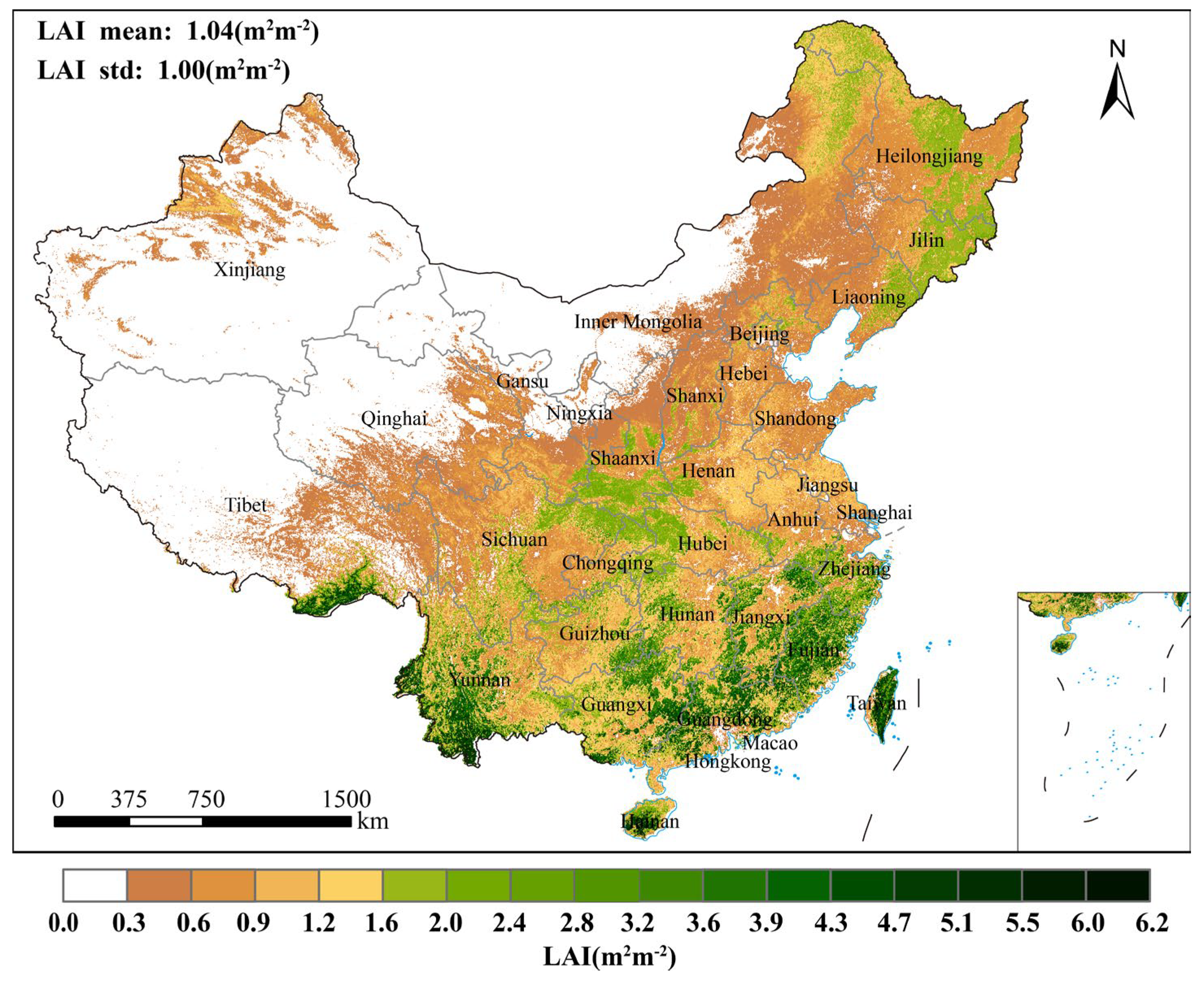
Figure 1. Temporal average of MODIS LAI in China, 25 June 2000 to 25 June 2022.
Remotesensing 15 02975 g001
Figure 2. VCA–MLC algorithm flowchart. The process of extracting vegetation endmembers was conducted 1000 times for the sample of MOD-2011, which was also used as the sample for subsequent MLC.
Remotesensing 15 02975 g002
Figure 3. China Vegetation Functional Zones (CVFZ) and location of the selected vegetation endmembers. The curve in the lower left corner corresponds to the color of the classification chart.
Remotesensing 15 02975 g003
Figure 4. Validation results of CVFZ and several land cover products. The proportion of each vegetation type was calculated to provide more information. (a) MCD-2011, (b) CLCD-2011, (c) MCD-unchanged, and (d) MCD-CVFZ (the legend of Figure 4d only shows areas with more than 10,000 pixels).
Remotesensing 15 02975 g004
Figure 5. The performance of CVFZ in distinguishing the LAI mean and LAI standard deviation of MOD-2011. The LAI mean for each vegetation type is represented by black dots, and the legend’s color scheme is consistent with Figure 3 (some zones are not distributed in all vegetation types).
Remotesensing 15 02975 g005
Figure 6. The performance of CVFZ in distinguishing LAI time series, 25 June 2000 to 25 June 2022. The legend’s color scheme is consistent with Figure 3.
Remotesensing 15 02975 g006
Figure 7. LAI time series and linear regression results of annual fluctuations, 25 June 2000 to 25 June 2022. The legend’s color scheme is consistent with Figure 3.
Remotesensing 15 02975 g007
Figure 8. LAI time series of intra-annual fluctuations, 25 June 2000 to 25 June 2022. The legend’s color scheme is consistent with Figure 3.
Remotesensing 15 02975 g008
Figure 9. The LAI mean and D2 (indicated by the error bar) in MCD-2011 and MCD-CVFZ in the same vegetation. The red curve represents the proportion of pixels remaining after MCD is cut.
Remotesensing 15 02975 g009
Figure 10. Spatial variability in vegetation dynamics revealed by CVFZ: a case study of the Hengduan Mountains, the Chengdu Plain, and the Sichuan Basin.
Remotesensing 15 02975 g010
Table 1. Extraction results of vegetation endmembers. The locations of endmembers are accurate to the province, and vegetation types are defined based on the MCD12Q1 type3 band.
P o c c u r r e n c e RowColumnLocationVegetation Type
100.0%16891724YunnanEvergreen Needleleaf Forests
3.9%18022707TaiwanSavannas
3.7%20902125HainanSavannas
2.2%18282707TaiwanSavannas
1.8%11312117ShaanxiDeciduous Broadleaf Forests
1.6%11652070GansuDeciduous Broadleaf Forests
1.5%7522754LiaoningGrasslands
1.2%12882178HenanGrasslands
1.1%17382556FujianEvergreen Broadleaf Forests
1.1%10632198ShanxiDeciduous Broadleaf Forests
Table 2. The adjustment of the Threshold of CVFZ induces a shift in the evaluation metrics (missing rate (MR), interclass distance (D1), in-class distance (D2), and discrimination (D3)). The identification of the optimal Threshold is predominantly dependent on D3.
Threshold2.022.032.042.052.062.072.08
MR0.07690.06330.04770.03180.02050.01340.0087
D10.25810.25770.25710.25670.25620.25570.2553
D20.20680.20630.20570.20510.20460.20420.2039
D30.05130.05140.05140.05160.05150.05150.0514
Disclaimer/Publisher’s Note: The statements, opinions and data contained in all publications are solely those of the individual author(s) and contributor(s) and not of MDPI and/or the editor(s). MDPI and/or the editor(s) disclaim responsibility for any injury to people or property resulting from any ideas, methods, instructions or products referred to in the content.