Rice False Smut Monitoring Based on Band Selection of UAV Hyperspectral Data

Abstract

Rice false smut (RFS) is a late-onset fungal disease that primarily affects rice panicle in recent years. Severe RFS can decrease the yield by 20–30% and severely affect rice quality. This research used hyperspectral remote sensing data from unmanned aerial vehicles (UAV). On the basis of genetic algorithm combined with partial least squares to select the feature bands, this paper creates a new method to use the Pearson correlation coefficient method and Instability Index between Classes (ISIC) method to further select characteristic bands, which further eliminated 27.78% of the feature bands when the model monitoring accuracy was improved overall. The prediction accuracy of the Gradient Boosting Decision Tree model and Random Forest model was the best, which were 85.62% and 84.10%, respectively, and the monitoring accuracy was improved by 2.22% and 2.4% compared with that before optimization. Then, based on the UAV hyperspectral data and the combination of characteristic bands selected by the three band optimization methods, the sensitive band ranges of rice false smut monitoring were determined, which were 698–800 nm and 974–997 nm. This paper provides an effective method of selecting characteristic bands of hyperspectral data and a method of monitoring crop diseases’ using unmanned aerial vehicles.

1. Introduction

Agriculture is the lifeline to all countries and the guarantee of food security for people around the world. In agriculture, rice is one of the most important crops and accounts for about 70 percent of global consumption. Rice is also considered one of the most important grains of every meal [1]. China is not only the world’s largest rice producer but also consumes and imports more rice than other countries, which means that the stability of Chinese rice production has a big impact on the global rice market [2]. Insect pests and diseases are the major causes of grain yield loss and quality decline in agricultural production. In addition to economic losses, insect pests and diseases also threaten global food security [3,4]. Rice will be exposed to various fungi during its growth and development which will lead to a serious decline in quality and yield. Rice false smut (RFS) is a late fungal disease caused by the ascomycete fungus which uses rice panicles as the primary host [5]. Recently, RFS has become a devastating disease in a good deal of major rice-producing countries including China, Japan, India and the United States [6,7]. RFS will consume the whole panicle nutritional of rice and result in a serious decline in rice quality and huge losses [8]. RFS reduces “thousand seed weight” and seed germination (by up to 35%). In wet weather, RFS may cause a production loss of up to 25%. After rice planting, the bacteria still survive in the soil and infect the seedlings [9]. Although RFS is mainly concentrated on small areas around the original disease source area, the common practice is still to spray pesticides indiscriminately on the entire field [10]. In order to minimize the economic losses and environmental pollution caused by pesticides, it is necessary to accurately assess the distribution and prevalence of RFS [11]. Therefore, an automated, non-destructive, fast, sensitive and selective method is urgently needed to quickly detect plant diseases and reduce the use of pesticides and fertilizers to support sustainable agricultural production [11,12].

Remote sensing technology [13,14] has shown unique advantages in crop disease and pest stress monitoring on account of its characteristics of accuracy, rapidity, extensive area and no damage [15]. Recently, remote sensing technology has made important contributions to large-area agricultural resource monitoring, crop to yield forecasting, agricultural situation forecasting, etc. [16,17]. In recent years, with the rapid development of the UAV industry, remote sensing of the UAV clothing industry has played an important role in the application of crop disease and pest stress monitoring on account of its characteristics of high spatial resolution of image, high timeliness of data acquisition and low cost [15,18]. Therefore, UAV hyperspectral photogrammetry is an effective method for rapid and accurate monitoring of small and medium-sized crop pests and diseases. In the literature, many researchers use UAV remote-sensing images to monitor crop pests and diseases. For example, high spatial resolution aerial images were used to monitor the invasion degree of yellow leaf spots on banana crops and the Support Vector Machine method was used to achieve good accuracy [19]. Multi-spectral cameras and unmanned aerial vehicles are used to get time series band aerial multispectral images, study spectral data on crops in different periods and get an effective method of monitoring early crop diseases and insect pests [20]. Apart from using high-resolution and multispectral images to monitor crop diseases and pests, hyperspectral images are also an important means to detect crop diseases and pests. Some researchers used hyperspectral imaging technology to identify tomato yellow leaf disease and used spectral characteristic parameters and spectral bands such as the first derivative reflectance spectrum and absolute reflectance difference spectrum to accurately monitor the disease situation of crops [21]. Some researchers also select characteristic spectral bands of hyperspectral bands to reduce the dimensions of hyperspectral data and get high accuracy [22,23,24]. However, in the research of monitoring crop pests and diseases based on hyperspectral images, most of the data acquisition methods are to use a ground hyperspectral imager to collect crop hyperspectral images which is difficult to achieve extensive area, rapid and accurate monitoring of crops.

In the research of monitoring crop pests and diseases using hyperspectral remote sensing images, usually people inoculate healthy crops with related diseases and pests to infect crops more evenly, which can do more detailed research on each stage of crop disease. However, in nature, pests and diseases infect crops from a few points to gradually infect nearby healthy crops, and the disease situation of crops is more complex. Therefore, in order to establish a more accurate monitoring model of crop pests and diseases, in addition to actively studying the changes of spectral characteristic curves of crop pests and diseases at various time periods, we also need to pay attention to the study of crops infected with diseases and pests in the natural environment. In the existing research, some use the machine learning classification method Support Vector Machine (SVM) and histogram analysis method [1,8,23] to select features, some use the neural network (CNN) to build models [25] for the whole band or use genetic algorithm [23,24] to extract feature bands. Many more researchers use the Random Forest (RF) model [3,11,20,22] to establish crop disease and pest detection models and achieve high accuracy. In summary, spectral analysis of hyperspectral images and calculation of spectral parameters are the primary methods for pest and disease monitoring, and the use of machine learning models and deep learning networks is a hot research direction.

Using hyperspectral remote sensing images to monitor crop pests and diseases and selecting bands of hyperspectral data is the direction to improve the accuracy of pest and disease monitoring. Some studies have been conducted to screen characteristic bands of hyperspectral bands based on the genetic algorithm and partial least squares method [26], some use the Guided Regularized Random Forest (GRRF) to screen hyperspectral bands [22] or use genetic algorithm combined with Support Vector Machine (SVM) to select hyperspectral bands [23]. Except for using model calculations to select characteristic bands, some researchers also select characteristic bands by processing raw spectral data. For example, some researchers use the principal component analysis method to reduce the dimensionality of the raw, inverse logarithmic, first and second derivative reflectance spectra [27]. Some researchers also select characteristic bands based on the hyperspectral characteristic band selection method established based on the instability index and improved stable zone unmixing [24]. Some researchers have also proposed a spectral feature extraction algorithm based on the linear discriminant analysis (LDA) and texture feature extraction based on integral images [28]. The minimum noise fraction algorithm (MNF), canonical correlation analysis (CCA), projection pursuit, orthogonal subspace projection (OSP) and discrete wavelet transform (DWT) are also classical hyperspectral data feature extraction algorithms [12]. However, the method used in the above studies only preliminarily selects the optimal feature bands, and the combination of feature bands is the local optimal combination. Therefore, this paper is pioneering in selecting the best combination of characteristic bands of a variety of band selection methods to improve the monitoring accuracy of rice false smut.

In summary, few studies have applied UAV hyperspectral data to rice false smut monitoring, and no effective monitoring method based on UAV hyperspectral photogrammetry has been developed. Therefore, the main objectives of this study are in two aspects: (1) To develop a band selection method of hyperspectral data to get the optimal combination of characteristic bands and (2) to develop a rapid and accurate monitoring method for rice false smut based on UAV hyperspectral photogrammetry.

2. Materials and Methods

2.1. Data Acquisition

2.1.1. Experimental Design and UAV Photogrammetry

The UAV flight platform (see Figure 1) used in this study was developed by Shenzhen DJI Innovation Technology Co., Ltd. (Shenzhen, China) with the model of Matrix 600 Pro. The UAV is equipped with three Inertial Measurement Unit (IMU) and Global Navigation Satellite System (GNSS) modules. This redundant system design can ensure the reliability and stability of the flight platform. In order to provide a stable working environment for the hyperspectral sensor and reduce the geometric distortion of the image caused by the vibration of the motor, the acceleration of the aircraft and the change of direction and route of the aircraft, a gimbal system equipped with a high-precision IMU (see

Table 1. Some technical parameters of DJI Pan-Tilt Ruying Ronin-MX.

Technical Parameter	Value
Maximum load weight	4.5 kg
Endurance time	180 min
Operating ambient temperature	−50 °C to 15 °C
Angular jitter	±0.02°

, Figure 1) is used in this study. The gimbal system used in this study is also the Ronin-MX developed by Shenzhen DJI Innovation Technology Co., Ltd. The hyperspectral imagery used is a visible near-infrared push-sweep hyperspectral imagery developed by Head Wall Company (Boston, MA, USA) in the United States, and the model is Nano-Hyperspec^® (see

Table 2. Some technical parameters of hyperspectral imager Nano-Hyperspec^®.

Technical Parameter	Value
Wavelength range	400–1000 nm
Number of pixels per row	640
Number of bands	270
Spectral resolution	2.2 nm
Operating ambient temperature	0–50 °C

, Figure 1).

Scientific and reasonable flight plan is the basis for obtaining high-quality data and improving data acquisition efficiency. Terrain conditions, weather conditions, the shape of the study area, the angle of view of the hyperspectral imager and other factors need to be contemplated. Finally, the optimal flight speed, flight altitude, exposure time and other parameters are determined (see

Table 3. Specifications of four UAV campaigns in this study.

Date	Speed	Altitude
14 August 2020	5.8 m/s	100 m
20 August 2020	6.8 m/s	100 m
25 August 2020	6.2 m/s	100 m
2 September 2020	6.0 m/s	100 m

). In this study, the UAV collected data on no wind or slight wind, no cloud or little cloud, stable lighting conditions and a large solar altitude angle (10:00–14:00). In addition, the reflectance calibration cloth is placed in the experimental area to facilitate the radiometric correction of images. The flight altitude of four UAV hyperspectral data acquisition experiments in this study is 100 m, and the spatial resolution of remote sensing image is 9.2 cm. The flight speed of the UAV shall be set according to the weather and it shall be calculated according to Equation (1).

$$\mathrm{v}=\frac{\mathrm{FOV}·\mathrm{h}}{\mathrm{n}·\mathrm{t}}$$

(1)

Here, v is the flight speed of the UAV imaging system, t is the exposure time, FOV is the field of view, h is the flight altitude and n is the number of pixels per row.

2.1.2. Field Measurement

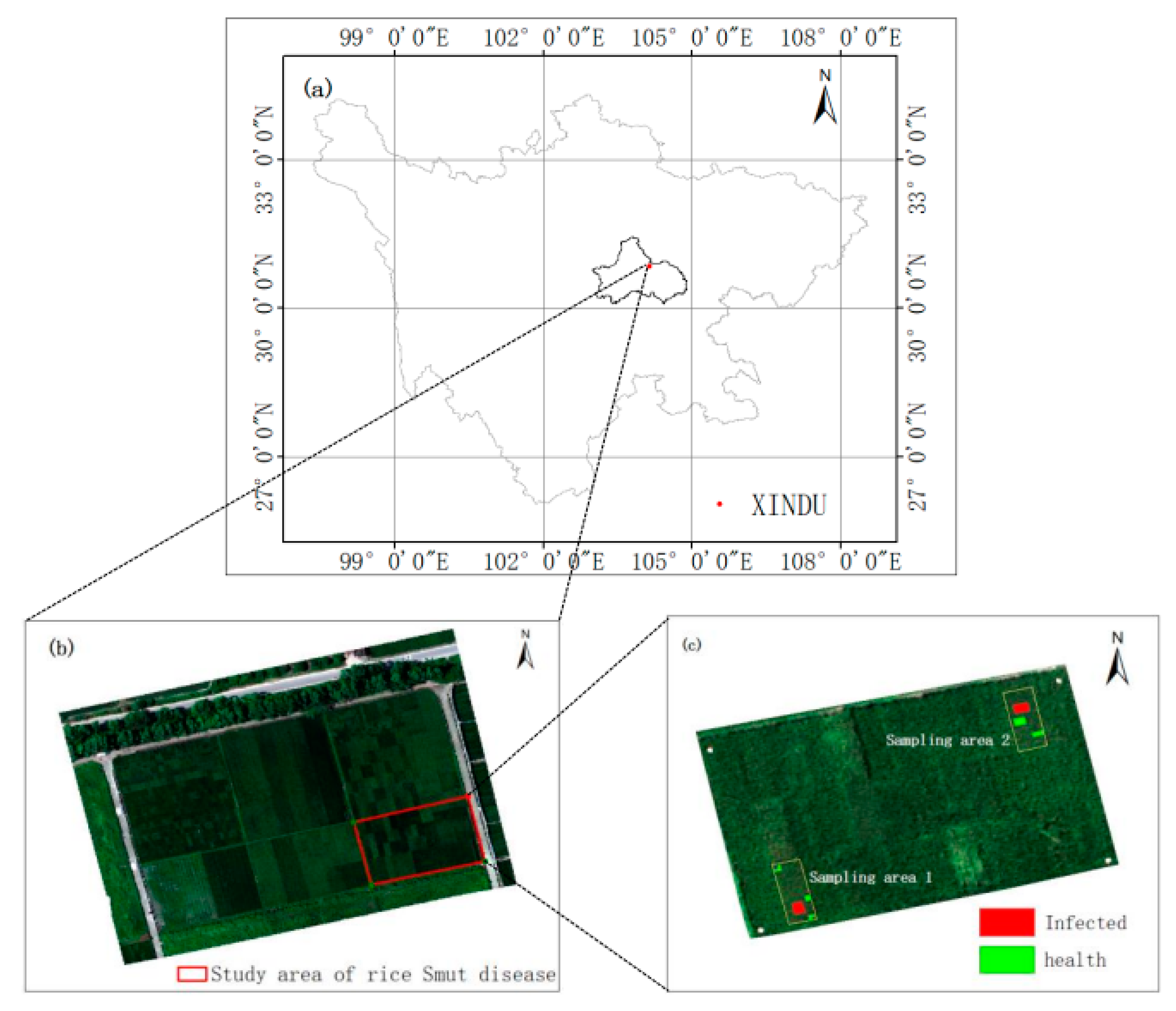
The research area reposes on the Modern Agricultural Science and Technology Innovation Demonstration Park of the Academy of Agricultural Sciences, Chengdu Xindu District, Sichuan Province (Figure 2a). Hyperspectral photogrammetry of rice in the research area was carried out using the UAV flight platform equipped with remote sensing equipment. Figure 2b,c shows the map covering the RGB top view of the rice field in the study area. The red box in Figure 2b shows the selected area of the study rice false smut. In Figure 2c, two sampling areas are marked, and the location information of the diseased area and the healthy area of rice are collected in sampling areas 1 and 2. There were among 36 experimental plots and 12 rice varieties in the rice false smut research area. Each rice variety was planted three times in duplicate and 252 litters of rice (9 rows × 28 rows) were planted in each plot. In the experimental field, the rice planting density was 26.67 cm × 20.00 cm and the same field management methods (such as irrigation method, fertilizer application rate, etc.).

The information data on the occurrence of RFS (including the diseased area and the healthy area) were collected as shown below: First, visually identify whether rice is infected with rice false smut or healthy, then use a tape measure to measure the distance between each border of the diseased area (or healthy area) and the border of the rice planting area and finally match with the UAV hyperspectral image to get the positions of healthy points and diseased points in the hyperspectral image. The idea of data collection for infected areas and healthy areas is to measure the infected area on the first day of data collection (If an area is infected at this moment, it means that the area is also infected later) and measure the healthy area on the last day (If an area is healthy at this moment, it means that the area was healthy before). The infected area was measured on 14 August 2020, and the infected area shape file collected on 14 August 2020 is also the shape file of the other three dates. The health region was measured on 2 September 2020 and the shape file of the health region collected on 2 September 2020 is also the shape file of the other three dates. Figure 2c shows the results of the field survey, which includes both healthy and rice false smut-infected areas. In the figure, the healthy area is marked with green and the infected area is marked with red. The center coordinates of the experimental site are Lat: 30°47′13″N, Lon: 104°12′16″E.

2.2. Data Preprocessing

2.2.1. Hyperspectral Data Filtering Processing

In this section, we mainly introduce the causes of hyperspectral data noise generation, explain the principle and characteristics of a Savitzky-Golay filter and explain the reasons for choosing the filter and the relevant parameter Settings of Savitzky–Golay filter.

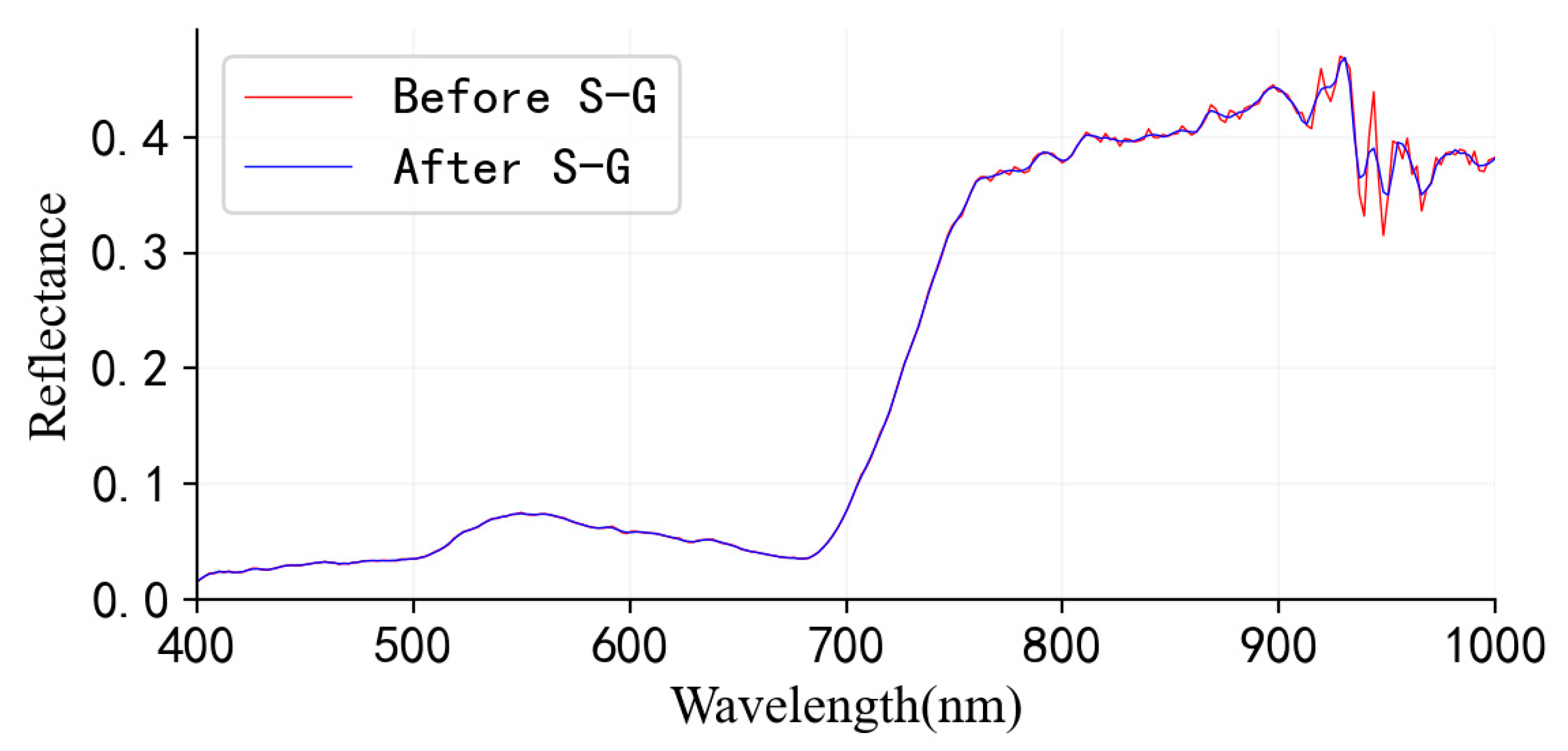
The hyperspectral data onto UAV has hundreds of bands, which can be used to photograph the ground object to a height of overtop 100 m. Sometimes, because the signal-noise ratio of the instrument does not reach the optimal working state or on account of the combined effect of dark current and other interfering factors, the spectral reflectivity of different wavebands has some noise, resulting in the reflectivity of adjacent wavebands showing zigzag characteristics (Figure 3). In order to get a smooth spectrum, improve the signal-to-noise ratio and improve the accuracy of information extraction, hyperspectral data need to be processed by spatial domain smooth filtering. There are two kinds of spatial smoothing filtering methods: linear and nonlinear. Linear smoothing includes mean filtering, Gaussian filtering, etc. Nonlinear smoothing includes median filtering, bilateral filtering and so on. Savitzky–Golay (S–G) filter is a low-pass filter, also known as S–G smoother. As S–G is a filtering method based on local polynomial least square fitting in the time domain, it can ensure the shape (maximum value, minimum value) and width distribution characteristics of the signal while filtering noise [29], so this paper chooses S–G filtering method for filtering hyperspectral data. S–G filter is a best-fitting method based on polynomials in time domain by moving Windows using the least squares method. When using S–G filtering, it is necessary to determine the applicable moving window size (positive odd number) and polynomial degree. The larger the value of the moving window, the smoother the spectral curve is, and some information will be lost. The smaller the moving window, the closer it is to the real curve. The larger the polynomial degree, the closer the curve is to the real curve. The smaller the curve, the smoother the curve. In addition, when the degree of the polynomial is large, due to the limitation of the window length, there will be problems with the fitting, and the high-frequency curve will become a straight line [29,30]. Therefore, this study adopts the S–G convolution smoothing method of moving window 9 and quadratic polynomial to smooth and dense hyperspectral data (Figure 3).

2.2.2. Acquisition of Rice False Smut Monitoring Database

The location data of rice false smut and the location data of healthy rice sampling points were matched in ENVI software to get the spectral reflectance data sampling points. We used the ROI tool by ENVI software to extract the data of the region of interest. According to the location data sampling points, we used the ROI tool to output the spectral reflectance of healthy and diseased sampling points of hyperspectral data collected on four dates, respectively and finally get the spectral database of rice false smut monitoring.

2.3. Hyperspectral Feature Band Optimization

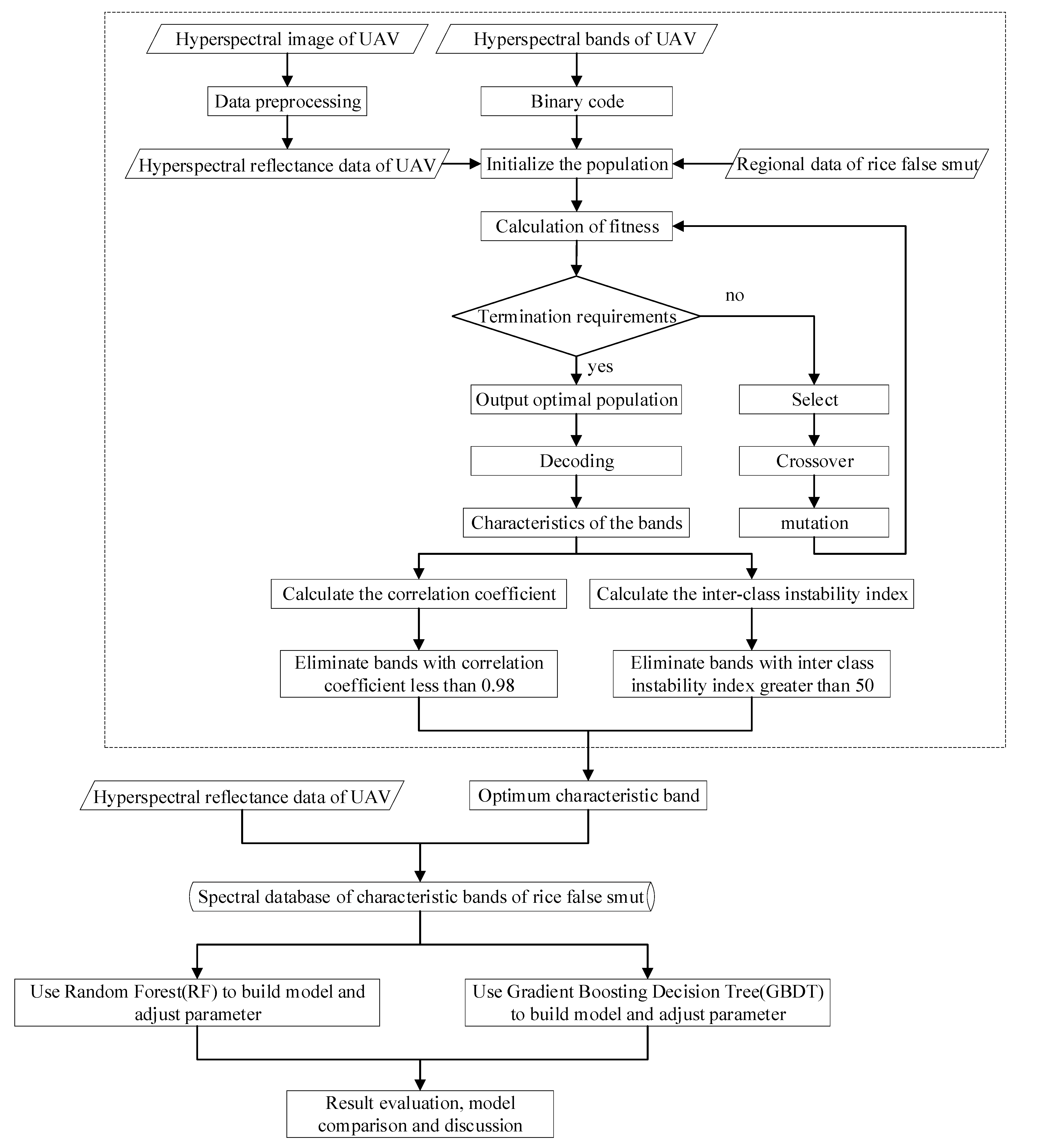
In this section, the following three parts, respectively introduce the basic principle of genetic algorithm, correlation coefficient method and inter-class instability index method and the specific process, technical details and parameter setting of characteristic band selection of UAV hyperspectral data. The dotted line box in Figure 4 specifically shows the operation flow of this section.

2.3.1. Hyperspectral Feature Band Optimization Based on Genetic Algorithm

The Genetic Algorithm (GA) adopts the natural evolution model, which is self-organizing, adaptive and self-learning. Genetic algorithms transform the original population of the parameter space by encoding, and the most important thing is to select an appropriate fitness function as the evaluation basis. The genetic algorithm takes the coded population as the initial population, realizes the selection and genetic mechanism for the genetic operation of genes in the population and finally establishes an iterative process to get the optimal solution [31]. The calculated flow of hyperspectral features band selection using genetic algorithm is as shown below:

• Step1: Generate the initial population. Taking the rice disease monitoring accuracy as the optimal object, the hyperspectral band was coded with binary code as the gene and the initial population was randomly generated.
• Step2: Selecting Fitness function. In the genetic algorithm, individual fitness is used to determine the probability of the individual being inherited to the next generation population. The greater the fitness of an individual, the greater the probability that the individual will be inherited to the next generation and vice versa [31]. Partial least squares cross test of mean square error (RMSECV) was used as the fitness function [23].
• Step3: Genetic algorithm parameter design. The main control parameters of genetic algorithm include population size, iteration times, mutation probability, crossover probability, etc. In addition, before the initial population is assigned, it should be estimated at a large probability interval to avoid the limitation of the search range of the genetic algorithm and reduce the burden on the algorithm at the same time. If the group size is too large, the results are difficult to converge and waste resources and the robustness decreases. If the mutation probability is too small and the population diversity declines too fast, it easily leads to the rapid loss of effective genes and is no picnic to repair. If the iteration of the genetic algorithm is too small, the algorithm will not converge easily; If the number of iterations is too large, the algorithm will lead to a premature population and further evolution will only increase time expenditure and waste of resources. If the mutation probability is too large, the diversity of the population can be guaranteed, but the better solution will be eliminated. Similar to the mutation probability, the crossover probability is easy to destroy the existing solution, increases the randomness and easily misses the optimal individual; In addition, if the crossover probability is too small, the genetic algorithm cannot effectively renew the population [32].
• Step4: Algorithm termination condition. When the fitness of the optimal band combination is no longer improved or the number of iterations of the genetic algorithm reaches the preset number of iterations, the operation is aborted. After repeated experiments and tests, the initial population size is set as 30, the crossover probability is 0.5, the mutation probability is 0.01 and the maximum iteration is 100 at this moment [26].

2.3.2. Hyperspectral Feature Band Optimization Based on Correlation Coefficient

Pearson correlation coefficient (PCC) [33] (r) is used to measure the correlation (linear correlation) between two variables X and Y, and its value is between −1 and 1, which is defined and calculated by Equation (2).

$$\mathrm{r}=\frac{{{\displaystyle \sum }}_{\mathrm{i}=1}^{\mathrm{n}}({\mathrm{X}}_{\mathrm{i}}-\overline{\mathrm{X}})\left({\mathrm{Y}}_{\mathrm{i}}-\overline{\mathrm{Y}}\right)}{\sqrt{{{\displaystyle \sum }}_{\mathrm{i}=1}^{\mathrm{n}}{\left({\mathrm{X}}_{\mathrm{i}}-\overline{\mathrm{X}}\right)}^2}\sqrt{{{\displaystyle \sum }}_{\mathrm{i}=1}^{\mathrm{n}}{\left({\mathrm{Y}}_{\mathrm{i}}-\overline{\mathrm{Y}}\right)}^2}}$$

(2)

In Equation (2), $\mathrm{r}$ is the Pearson correlation coefficient, $\overline{\mathrm{X}}$ and $\overline{\mathrm{Y}}$ are the mean values of variables X and Y and ${\mathrm{X}}_{\mathrm{i}}$ and ${\mathrm{Y}}_{\mathrm{i}}$ are the element values of variables X and Y.

The value of the coefficient is 1, it means that X and Y can be well described by the linear equation. All data fall on a straight line and Y increases with the increase of X [34,35]. When the correlation coefficient of the two variables is close enough to 1, the two variables can be considered to be strictly linearly correlated. Therefore, the information on one of the two linearly correlated bands can be used to place the information on the two bands with the monitoring of rice false smut. Because these two bands are strictly linearly correlated, the information lost by eliminating one band is limited and mutual interference with related bands can be avoided during model checking. In this way, the original data can be compressed and noise data can be reduced under the premise of retaining the original information as much as possible.

Therefore, based on the principle that the two variables with large correlation can be expressed linearly to each other, the correlation coefficient method is used to select the hyperspectral band. We eliminate the variables whose correlation is greater than a certain threshold to ensure that the correlation coefficients between the remaining variables are less than the threshold. When Pearson’s correlation coefficient is between 0.8 and 1.0, variables X and Y are strongly correlated [36]. In this paper, the correlation coefficient between bands selected by the genetic algorithm is firstly calculated and a threshold between 0.8 and 1.0 is selected as the criterion for the correlation coefficient selection of hyperspectral bands. After each threshold is selected, bands that did not meet the threshold conditions are eliminated from the preliminary preferred bands and the monitoring model is constructed using the preferred bands and the prediction accuracy is calculated. Finally, the correlation coefficient threshold with the highest prediction accuracy is acquired.

2.3.3. Hyperspectral Feature Band Optimization Based on Instability Index between Classes

The Instability Index between Classes (ISIC) is an important index for quantitative evaluation of the separability of samples of each band of hyperspectral data. ISIC can judge the applicability of a band to the second or multi classification problem by the size of the ISIC and then select some bands that are suitable for the sake of related classification or eliminate the bands that are not suitable for related classification. ISIC is calculated in sequence by the band, and the instability index of each band is calculated in sequence by taking the same band of various samples as the unit. When there are two types of samples involved in the operation, the ISIC can be calculated from Equation (3) [24].

$${\mathrm{ISIC}}_{\mathrm{i}}=\frac{\mathsf{\Delta }\mathrm{within},\mathrm{i}}{\mathsf{\Delta }\mathrm{between},\mathrm{i}}=\frac{{\mathrm{S}}_{1,\mathrm{i}}+{\mathrm{S}}_{2,\mathrm{i}}}{\left|{\mathrm{m}}_{1,\mathrm{i}}-{\mathrm{m}}_{2,\mathrm{i}}\right|}$$

(3)

In Equation (3), ${\mathrm{ISIC}}_{\mathrm{i}}$ is the Instability Index between Classes of two types of samples at the i-th band; $\mathsf{\Delta }\mathrm{within},\mathrm{i}$ and $\mathsf{\Delta }\mathrm{between},\mathrm{i}$ is the intra class deviation and inter class deviation, respectively; ${\mathrm{S}}_{1,\mathrm{i}}$ is the standard deviation of the first type samples at the $\mathrm{i}$-th band, and ${\mathrm{S}}_{2,\mathrm{i}}$ is the standard deviation of the second type samples at the $\mathrm{i}$-th band; ${\mathrm{m}}_{1,\mathrm{i}}$ is the mean value of the first type of sample in the i-th band, and ${\mathrm{m}}_{2,\mathrm{i}}$ Is the mean value of the second type of sample in the youth band. It can be seen from Equation (3) that when the intra-class deviation is smaller and the inter-class deviation is larger, the Instability Index between Classes is smaller [24].

If the number of categories of samples to be classified is greater than two, the Instability Index between Classes can be calculated by Equation (4) [37].

$${\mathrm{ISIC}}_{\mathrm{i}}=\frac{\mathsf{\Delta }\mathrm{within},\mathrm{i}}{\mathsf{\Delta }\mathrm{between},\mathrm{i}}=\frac{\mathrm{m}}{\mathrm{m}\left(\mathrm{m}-1\right)}{{\displaystyle \sum }}_{\mathrm{z}=1}^{\mathrm{m}-1}{{\displaystyle \sum }}_{\mathrm{j}=\mathrm{z}+1}^{\mathrm{m}}\frac{{\mathrm{S}}_{\mathrm{z},\mathrm{i}}+{\mathrm{S}}_{\mathrm{j},\mathrm{i}}}{\left|{\mathrm{m}}_{\mathrm{z},\mathrm{i}}-{\mathrm{m}}_{\mathrm{j},\mathrm{i}}\right|}$$

(4)

In Equation (4), $\mathrm{m}$ is the number of categories, ${\mathrm{S}}_{\mathrm{z},\mathrm{i}}$ is the standard deviation of the $\mathrm{z}$-th sample in the $\mathrm{i}$-th band and ${\mathrm{S}}_{\mathrm{j},\mathrm{i}}$ is the standard deviation of the $\mathrm{j}$ class sample in the $\mathrm{i}$-th band; ${\mathrm{m}}_{\mathrm{z},\mathrm{i}}$ is the mean of the $\mathrm{z}$-th sample in the $\mathrm{i}$-th band, and ${\mathrm{m}}_{\mathrm{j},\mathrm{i}}$ is the mean value of the $\mathrm{j}$ sample in the $\mathrm{i}$-the band.

The ISIC is an important index for characterizing the separability of each category in the band. According to the size of the ISIC, it can directly determine whether a band is conducive to more accurate classification of samples. When the standard deviation ${\mathrm{S}}_{\mathrm{z},\mathrm{i}}$ in each category is smaller, it manifests that the spectral reflectance of each sample of the same category is closer and the dispersion degree of the data is smaller. Therefore, the smaller the intra-class deviation ∆within is, the better the classification of samples. When the absolute value of the mean difference of $\left|{\mathrm{m}}_{\mathrm{z},\mathrm{i}}-{\mathrm{m}}_{\mathrm{j},\mathrm{i}}\right|$ is larger, it manifests that the greater the difference of spectral reflectance of each sample between different categories and the better the separability of spectral data. Therefore, the greater the inter class deviation $\mathsf{\Delta }\mathrm{between}, \mathrm{i}$, the more conducive to sample classification. In conclusion, the smaller the ISIC is, the better the classification accuracy will be. It is necessary to select the band of the smaller ISIC for monitoring, eliminate the band of the larger ISIC, further reduce the data dimension and improve the efficiency and accuracy of the model.

The most important thing is to select the threshold value of the hyperspectral feature band by using the method of ISIC. The larger the threshold is, the more hyperspectral bands are selected. Conversely, the number of preferred hyperspectral bands is smaller. In addition, when the threshold is too large or too small, it is easy to reduce the classification accuracy. So, it is necessary to find an optimal threshold as the criterion of band optimization. The search for the optimal threshold can be selected within the interval of ISIC aggregation. First, set a certain step size and then select the optimal band within the threshold interval with a certain threshold value. Finally, use the selected optimal band to establish a prediction model and then evaluate the accuracy to determine the optimal threshold value. In order to find the optimal threshold, a series of thresholds need to be selected. At the beginning, the step size can be set larger, the interval selected by the threshold can be narrowed according to the prediction accuracy calculated by the selected threshold, and then the optimal threshold can be acquired by setting a smaller step size. This method can effectively reduce the optimal threshold searching time. In this paper, prediction accuracy was used as the evaluation index of prediction accuracy. After selecting a series of thresholds in the threshold interval, the hyperspectral band was selected to establish the prediction accuracy of the rice false smut prediction model by comparing the ISIC with the threshold value.

2.4. Model Establishment and Verification

The data set is divided into a training set for model establishment and a verifiable set for model accuracy test by 7:3. The sample data set in this paper includes 1527 disease and health sampling points including 766 health sampling points and 761 disease sampling points. The sampling point data is uniformly collected from the five sampling areas in Figure 2c. It showed sample data set division in the following

Table 4. Data set partitioning.

	Number of Sampling Points	Training Set	Validation Set
no-m1	280	196	84
no-m2	170	119	51
no-m3	104	73	31
no-m4	111	78	33
no-m5	105	73	32
yes-m1	428	300	128
yes-m2	335	235	199
Total	Health	539	231
	Infected	535	327

In Table 4, yes and no indicate whether they are ill, and m1–m5 is the sampling area number.

:

In order to further verify the effectiveness of the hyperspectral band optimization method, a model between rice health and spectral data was established based on Random Forest and Gradient Boosting Decision Tree. The two models have unique characteristics. Through the mutual verification of various models, the optimal selection results of spectral bands can be comprehensively evaluated. Random Forest (RF) is an algorithm based on classification tree [38]. Random Forest improves the prediction accuracy of the model by summarizing many classification trees and has a fast computation speed and excellent performance in processing big data. In addition, Random Forest does not need to worry about the problem of multivariate collinearity, so it is easy to calculate the nonlinear effect of variables and can reflect the interaction between variables [39]. Gradient Boosting Decision Tree (GBDT) is a part of the ensemble boosting algorithm. GBDT can flexibly process various types of data including continuous values and discrete values. When using some robust loss functions, the robustness to outliers is very strong [40].

This study is to monitor whether rice suffers from rice false smut which is a binary problem. According to the combination of sample and model prediction categories, the four cases of the table are divided into the following

Table 5. Confusion matrix.

	Predicted Results
Real Situation	Positive Example	Negative Example
positive example	TP (True positive example)	FN (False negative example)
negative example	FP (False positive example)	TN (True negative example)

In Table 5, TP refers to the number of positive cases in the predicted results and the actual cases; FP refers to the number of actual cases that are counterexamples but are predicted to be positive; TN is the number of counterexamples in the prediction result and the actual situation; FN is the number of genuine cases as counterexamples but predicted as positive cases [41].

“confusion matrix” [41]:

Based on confusion matrix, accuracy, precision, recall and F1 score were used as evaluation indexes of the model in this study. Accuracy is how many samples are predicted correctly in all samples, see Equation (5); precision is how many of the predicted positive examples are actually positive, as shown in Equation (6); recall is how many samples of actual positive examples are predicted to be positive, see Equation (7); Accuracy and recall balances F1 score together, and F1 score combines these two quantities to improve decision-making speed, as shown in Equation (8). In order to better realize the monitoring and prevention of rice false smut, it is necessary to accurately extract the affected area of rice false smut, and the FP (False positive example) should be as small as possible. The evaluation index mainly refers to the accuracy and accuracy rate.

$$\mathrm{accuracy}=\frac{\mathrm{TP}+\mathrm{TN}}{\mathrm{TP}+\mathrm{FP}+\mathrm{TN}+\mathrm{FN}}$$

(5)

$$\mathrm{precision}=\frac{\mathrm{TP}}{\mathrm{TP}+\mathrm{FP}}$$

(6)

$$\mathrm{recall}=\frac{\mathrm{TP}}{\mathrm{TP}+\mathrm{FN}}$$

(7)

$$\mathrm{F}1=\frac{2\ast \mathrm{precision}}{\mathrm{precision}+\mathrm{recall}}$$

(8)

3. Results

3.1. Screening Results of Spectral Characteristic Bands by Genetic Algorithm

In this section, we introduce the detailed process of using genetic algorithms to select feature bands including the effect of band selection.

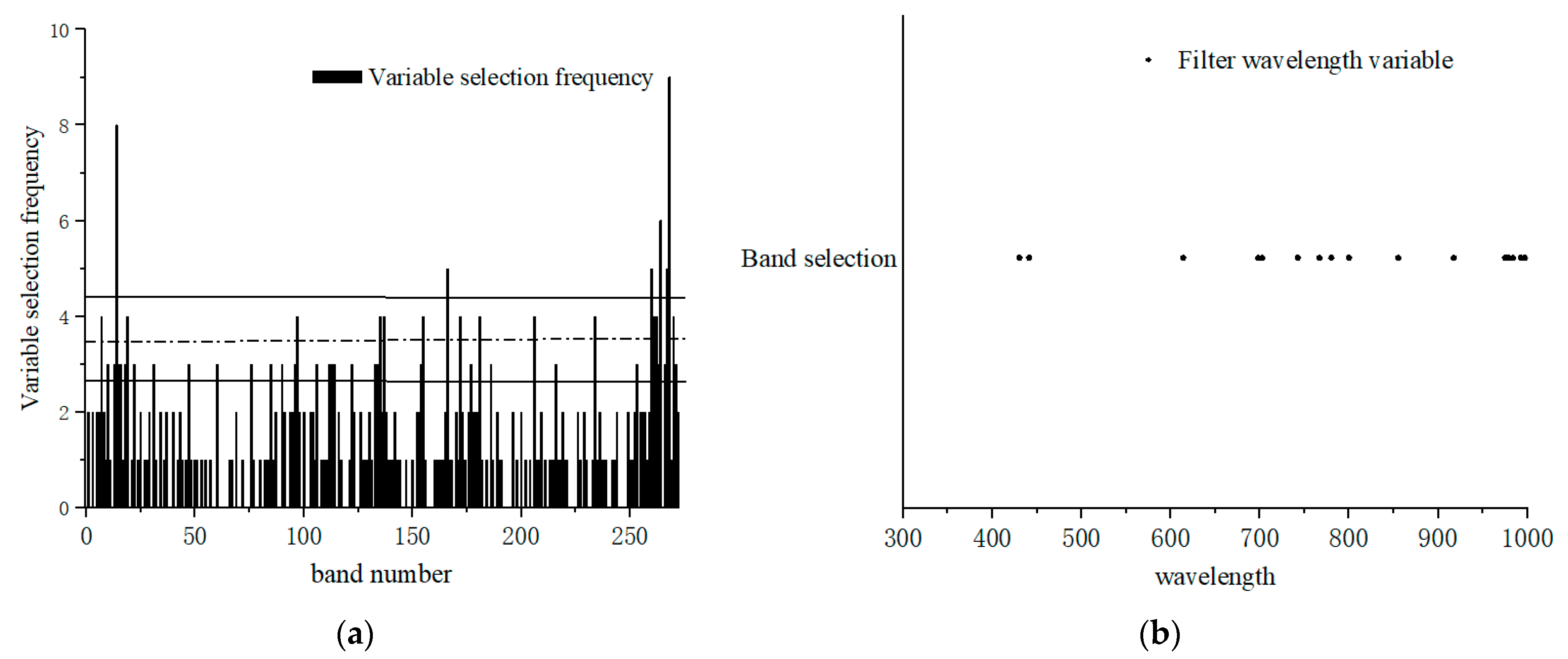
Using the data of 1527 hyperspectral samples of health and disease, a genetic algorithm combined with the partial least squares method was used to calculate and repeat the preprocessed spectral reflectance value 20 times, and the characteristic spectral bands were screened from 273 bands of hyperspectral images. Figure 5 shows the results of the spectral band screening operation of the genetic algorithm. The hyperspectral band range is 400–1000 nm, and there are 273 bands in total. The abscissa is the number of 273 bands according to the wavelength from small to large, and the ordinate is the frequency selected for each band in the 20-th band screening. On the variable selection frequency of Figure 5, there are three horizontal lines, which indicate that the characteristic band with the selected frequency greater than the horizontal line value is used for modeling. The position of a horizontal line is selected according to the accuracy of the model, and the optimal band combination with the best accuracy is selected as the result of band selection. In the figure, the number of feature bands selected by taking the top horizontal line as the reference is 8, the number of feature bands selected by taking the middle horizontal line as the reference is 18 and the number of feature bands selected by taking the bottom horizontal line as the reference is 42.

Then, we used three horizontal lines, respectively to screen out the feature band random forest model for verification. When eight characteristic bands were used for modeling, the prediction accuracy of the model was 76.91%. When 18 feature bands were used for modeling, the prediction accuracy of the model was 83.44%. When 42 feature bands were used for modeling, the prediction accuracy of the model was 83.44%. In this paper, 18 feature bands (the number of modeling bands accounts for 6.59% of the total spectral bands) screened based on the middle horizontal line were selected for modeling analysis and subsequent band screening.

According to the band selection results of genetic algorithm (see Figure 5b and

Table 6. Genetic algorithm optimization feature bands.

Preferred band number	7, 14, 19, 97, 135, 137, 155, 166, 172, 181, 206, 234, 260, 261, 262, 264, 268, 270
Preferred band wavelength	414.817 nm, 430.309 nm, 441.375 nm, 614.006 nm, 698.107 nm, 702.534 nm, 742.372 nm, 766.717 nm, 779.996 nm, 799.915 nm, 855.245 nm, 917.215 nm, 974.758 nm, 976.972 nm, 979.185 nm, 983.611 nm, 992.464 nm, 996.891 nm

), the selected characteristic bands are mainly 698–800 nm and 974–997 nm, which are consistent with the sensitive bands of RFS studied [11,27].

3.2. Screening Results of Spectral Characteristic Bands by Correlation Coefficient

In this section, we mainly show the calculation results of correlation coefficients and the detailed process of using correlation coefficients to select feature bands and analyze the rationality of selecting feature bands by correlation analysis.

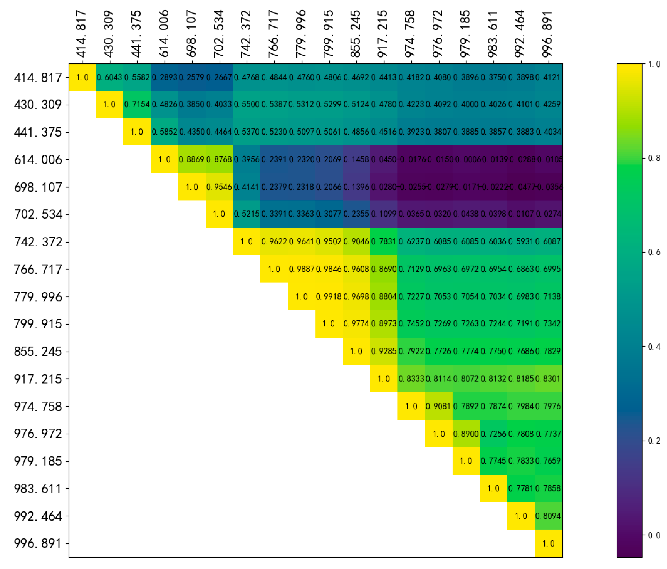
We use the preprocessed hyperspectral data to calculate the Pearson correlation coefficient between the 18 characteristic bands screened by the genetic algorithm to form a correlation coefficient matrix (Figure 6). Then, we need to analyze the correlation coefficient between the variables of each band and select an appropriate threshold to eliminate the relevant bands. The appropriate threshold value is determined by the prediction accuracy calculated by establishing the model of the optimized characteristic band, and the optimal threshold value is finally 0.98 after a series of operations. On the basis of the characteristic bands screened by the genetic algorithm, the bands of correlation coefficients greater than 0.98 are eliminated. Finally, 16 characteristic bands (the number of characteristic bands accounts for 5.86% of the total spectral bands) are acquired, which is 11.11% less dimensionality than the genetic algorithm-optimized characteristic band data.

According to the correlation coefficient of bands (see Figure 6), redundant bands with a high correlation coefficient are eliminated (see

Table 7. Correlation coefficient optimizes characteristic bands.

Preferred band number	7, 14, 19, 97, 135, 137, 155, 181, 206, 234, 260, 261, 262, 264, 268, 270
Preferred band wavelength	414.817 nm, 430.309 nm, 441.375 nm, 614.006 nm, 698.107 nm, 702.534 nm, 742.372 nm, 799.915 nm, 855.245 nm, 917.215 nm, 974.758 nm, 976.972 nm, 979.185 nm, 983.611 nm, 992.464 nm, 996.891 nm

), and the eliminated redundant bands are consistent with the range of redundant bands in other studies [42].

3.3. Screening Results of Spectral Characteristic Bands by Instability Index between Classes

In this section, we introduce the fundamental process of using the ISCI method to select the feature bands and analyze the rationality of the feature band selection results and the effectiveness of the ISCI method.

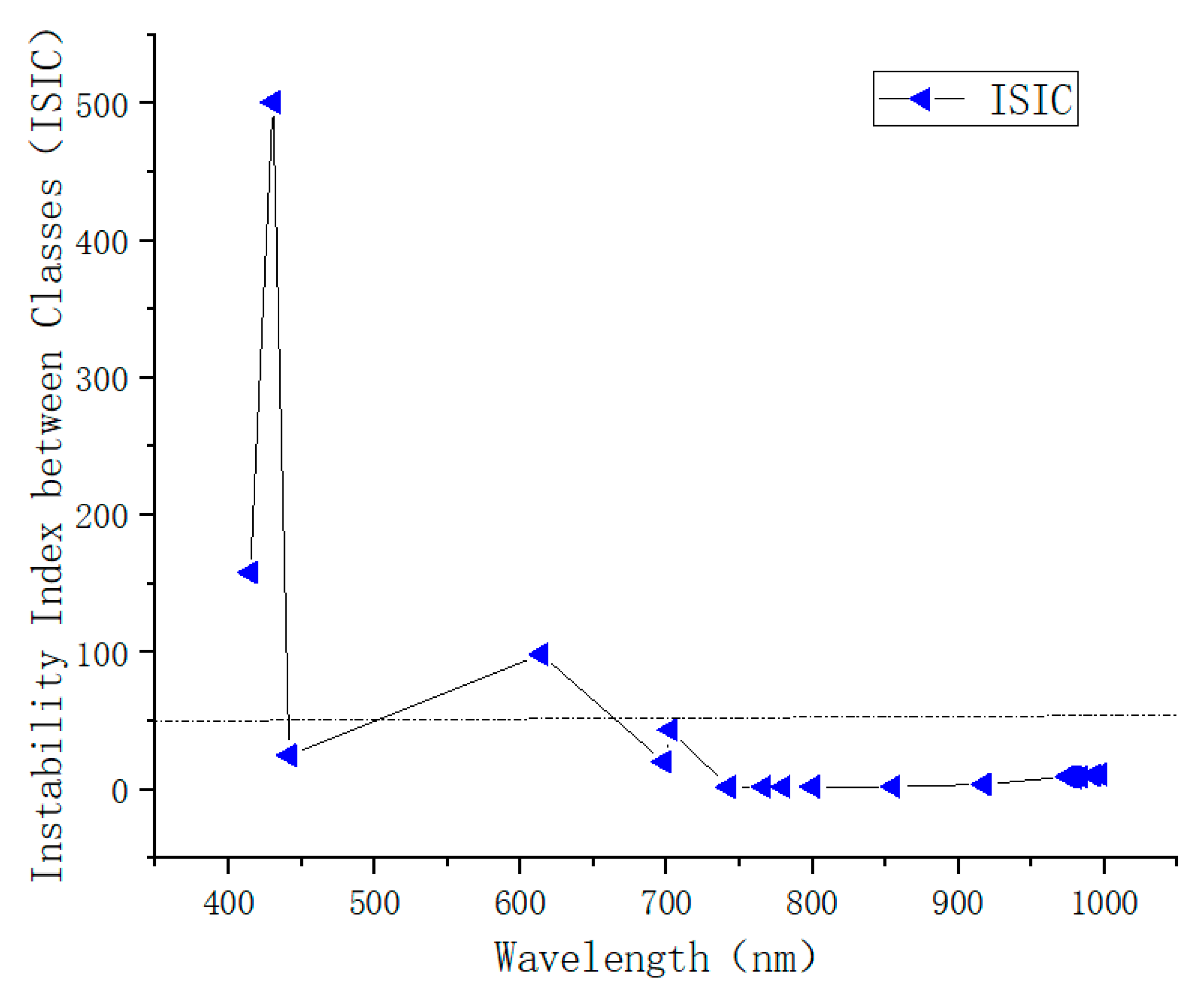
We use the preprocessed hyperspectral data to calculate the ISIC of 18 characteristic bands screened by genetic algorithm and select the appropriate threshold to eliminate the bands. According to the prediction accuracy of the model established by the filtered bands, this paper selects 50 as the screening threshold of the ISIC. On the basis of the characteristic bands screened by genetic algorithm, the bands with ISIC greater than 50 are eliminated. Finally, 15 characteristic bands (the number of characteristic bands accounts for 5.49% of the whole band) are acquired, which is 16.67% less dimensionality than the genetic algorithm optimized characteristic band data.

According to the ISCI calculation results (see Figure 7), 50 is selected as the threshold of eliminating bands, and bands larger than the threshold are eliminated (see

Table 8. Instability Index between Classes optimizes characteristic bands.

Preferred band number	19, 135, 137, 155, 181, 206, 234, 260, 261, 262, 264, 268, 270
Preferred band wavelength	441.375 nm, 698.107 nm, 702.534 nm, 742.372 nm, 799.915 nm, 855.245 nm, 917.215 nm, 974.758 nm, 976.972 nm, 979.185 nm, 983.611 nm, 992.464 nm, 996.891 nm

), which are all outside the range of sensitive bands given by existing studies [27].

3.4. Model Test

In Section 3.1, Section 3.2 and Section 3.3, genetic algorithm (GA), Pearson correlation coefficient (PCC) and Instability Index between Classes (ISIC) were used, respectively to select feature bands. In this section, based on the above results, the optimal characteristic bands selected by GA, GA + PCC, GA + ISIC and GA + PCC + ISIC were, respectively constructed by RF and GBDT models to verify the band selection results. Then, we use the accuracy evaluation index to evaluate the predicted results of the model. The accuracy evaluation results of the model are as shown below:

The Random Forest model was used to evaluate the characteristic bands selected by various methods. The characteristic bands were used to establish a model to predict the evaluation indexes according to Equations (5)–(8). The results are shown in

Table 9. Random Forest (RF) model.

Method	GA 1	PCC 2	ISIC 3	PCC + ISIC
Accuracy	83.44%	84.10%	84.10%	85.62%
Precision	79.84%	80.08%	80.08%	81.54%
Recall	89.57%	90.87%	90.87%	92.17%
F1-score	0.84	0.85	0.85	0.87
Excluded wavelength		766 nm, 779 nm	414 nm, 430 nm 614 nm	414 nm, 430 nm 614 nm, 766 nm 779 nm
Number of selected bands	18	16	15	13

¹ Genetic algorithm. ² Pearson correlation coefficient. ³ Instability Index between Classes.

. The correlation coefficient and the ISIC method eliminated two and three bands, respectively, and the accuracy, precision, recall and F1 scores were significantly improved compared to those before the elimination of bands. When five bands were eliminated in the meantime, the optimized feature band combination reduced the data volume by 27.8% on the basis of the original optimized feature band, and ensured that the accuracy, precision, recall and F1 score were significantly improved compared with the band elimination before band elimination and the band elimination by single method. The accuracy and precision can be improved by 2.22% and 1.70%, respectively by using correlation coefficient and ISIC to eliminate bands.

The optimal bands screened by various methods were evaluated based on Gradient Boosting Decision Tree model, and the evaluation indexes were calculated according to Equations (5)–(8). The results are shown in

Table 10. Gradient Boosting Decision Tree (GBDT) model.

Method	GA 1	PCC 2	ISIC 3	PCC + ISIC
Accuracy	81.70%	84.53%	82.79%	84.10%
Precision	77.86%	81.42%	78.93%	79.85%
Recall	88.70%	89.57%	89.57%	91.30%
F1-score	0.83	0.85	0.83	0.85
Excluded wavelength		766.717 nm, 779.996 nm	414.817 nm, 430.309 nm, 614.006 nm	414.817 nm, 430.309 nm 614.006 nm, 766.717 nm 779.996 nm
Number of selected bands	18	16	15	13

¹ Genetic algorithm. ² Pearson correlation coefficient. ³ Instability Index between Classes.

. For the optimal band selected by the correlation coefficient method and ISIC, the accuracy, precision, recall and F1 score have been improved. When the five bands screened by correlation coefficient and ISIC were removed in the meantime, the accuracy increased by 2.4% and the recall increased by 1.99%.

3.5. Monitoring Results of Rice False Smut

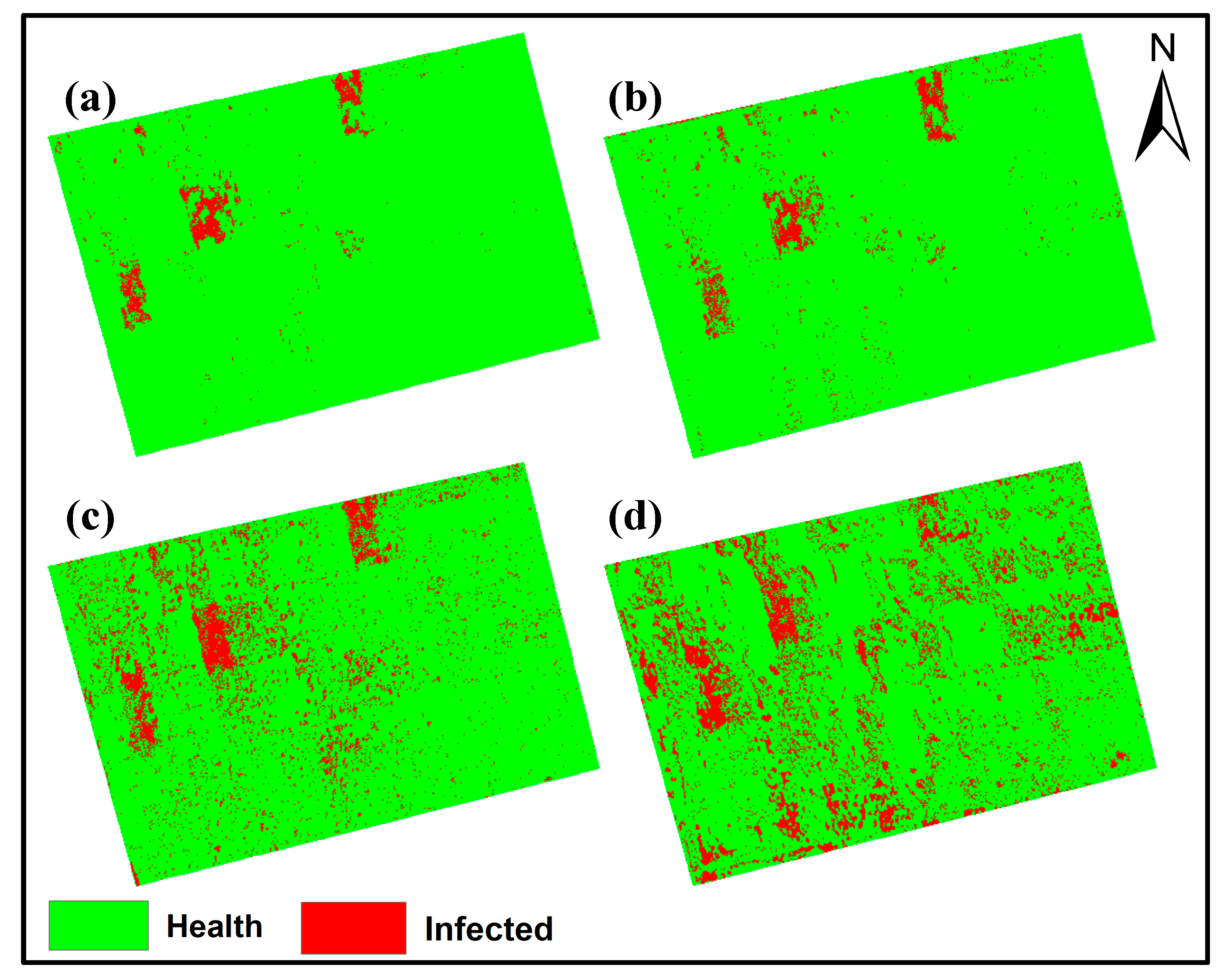
According to the results of the model test, the prediction accuracy of the Random Forest model based on the characteristic bands selected by the genetic algorithm, ISIC method and the correlation coefficient method is the best. Therefore, based on the UAV hyperspectral photogrammetry data of four periods, the random forest model trained in the model test in Section 3.4 was used to monitor rice false smut. The monitoring results of rice false smut are shown in Figure 8.

As shown in Figure 8a, on 14 August, rice in a few regions was extensively infected with rice false smut, while in other regions only a small area was affected; As shown in Figure 8b, six days later, on 20 August, a small area of diseased areas began to infect nearby healthy rice, but the infection rate was relatively slow; As shown in Figure 8c,d, a large area of disease began on 25 August and 2 September. The small area of disease in the front also rapidly infected nearby healthy rice, and rice fields were infected with rice false smut in an all-round way. Figure 8a,b are in the early heading stage of rice, so the infection rate of rice false smut is slow; As shown in Figure 8c,d, the period is at the rapid heading stage of rice, so rice false smut quickly infects the entire rice field. Therefore, for the monitoring of rice false smut, the earlier the discovery time is, the better the disease control is. The early heading stage of rice is an important time point for the control of rice false smut.

4. Discussion

In the study of monitoring crop diseases and pests with hyperspectral remote sensing images, people usually inoculate healthy crops with related diseases and pests to make the crops more evenly infected, so that more detailed studies can be conducted on each stage of crop diseases and pests [3,20]. However, in nature, pests and diseases infect crops from several points and gradually infect nearby healthy crops, and crop diseases and pests are more complex. The rice false smut disease studied in this paper is a random disease under natural infection, which is strikingly different from artificial inoculation in the laboratory. In the aspect of monitoring methods of crop diseases and insect pests, most researchers build models based on band selection of hyperspectral and spectral characteristic parameters (first derivative, etc.) [21,22,23,24]. However, the characteristic band selected by the method adopted in the above research is not optimal. In order to further improve the monitoring accuracy of crop diseases and pests, we need to optimize the band selection method. This paper monitors rice false smut based on band optimization of UAV hyperspectral data. According to the optimized characteristic band and model prediction results, the following outcomes are acquired through observation and analysis.

As shown in Table 6, Table 7 and Table 8, most of the selected characteristic bands are distributed in 698–800 nm and 974–997 nm, which are taken as sensitive bands in this paper. Based on the characteristic bands selected in Section 3.1, the correlation coefficient method is used to eliminate the redundant bands in Section 3.2 and the eliminated redundant bands are within the range of sensitive bands that have been given in existing studies. Furthermore, in Section 3.3, the ISIC method is used to eliminate insensitive bands, which are not within the range of sensitive bands that are given in existing studies. The above results are consistent with existing studies [11,27]. According to the existing studies on the hyperspectral reflectance of diseased rice panicles, the diseased rice ear will decrease greatly after 700 nm [27,43,44,45]. The reason for the above phenomenon is that rice leaves mainly absorb and reflect visible wavelengths, while rice ears are sensitive to the wavelength range after 700 nm. Therefore, the sensitive band range determined by the disease state of rice ears is after 700 nm, which is consistent with the sensitive band range obtained in this paper.

Observing the model test results in Table 9 and Table 10, we can find that after band selection by the correlation coefficient method and instability index between classes method, the monitoring accuracy of the model improved. By comparing the variation of model monitoring accuracy when the PCC is used to select bands, we can conclude that the selection of bands with strong correlation will reduce the model monitoring accuracy. In addition, by comparing the variation of monitoring accuracy when ISIC is used to select bands, we can conclude that the difference in spectral characteristics between diseased and healthy rice is useful information for monitoring rice false smut.

According to the verification results of RF and GBDT models, the correlation coefficient method and ISIC method can accurately screen the feature bands to achieve the purpose of reducing data volume and data noise (see Table 9 and Table 10). Because Random Forest (RF) can reflect the interaction between variables, the multivariate collinearity problem is not considered [39]. Therefore, after the correlation coefficient method is used to eliminate some strongly correlated bands, the prediction accuracy of the model is limited to improve. The Gradient Boosting Decision Tree (GBDT) can automatically combine the features and fit the nonlinear data. Therefore, the prediction accuracy of the model is greatly improved after the band is eliminated by the correlation coefficient method. In the meantime, the ISIC method can improve the accuracy of model monitoring by eliminating the insensitive band. Therefore, both PPC and ISIC methods can be used for feature band selection.

In this study, both the PCC method and the ISIC method we used needed to determine the appropriate thresholds. The prediction accuracy of the RF and GBDT models has been improved after the characteristic bands are further optimized by using the PCC method and ISIC method (see Table 9 and Table 10). The correlation coefficient method uses one of two strongly correlated variables to replace these two variables, which theoretically will lose important classification information, but may also eliminate noise data that hinder correct classification [33]. Therefore, whether the correlation coefficient threshold is reasonable determines the monitoring accuracy of rice false smut. ISIC is to select the characteristic bands according to the separability within the bands. The bands with larger ISIC are not conducive to accurate classification. Theoretically, removing bands with large ISIC will improve the prediction accuracy, but too small threshold setting will lose too much information, leading to a decline in classification accuracy. Similarly, whether the ISIC threshold is reasonable also determines the accuracy of rice false smut monitoring. Therefore, based on the principle of band selection by the two methods, both PPC and ISIC methods can be applied to select feature bands, but the selection of threshold values in the two methods greatly affects the monitoring accuracy of the model.

As shown in Table 9 and Table 10, comparing the prediction accuracy of the models with the same data, we found that the overall prediction accuracy of the RF model was higher than that of the GBDT model. However, in the same case, after further screening of feature bands, the accuracy of the gradient lifting tree model is higher than that of the random tree model. Therefore, the stochastic forest model has better monitoring accuracy of the whole, but the gradient lifting tree model has greater potential to improve the accuracy.

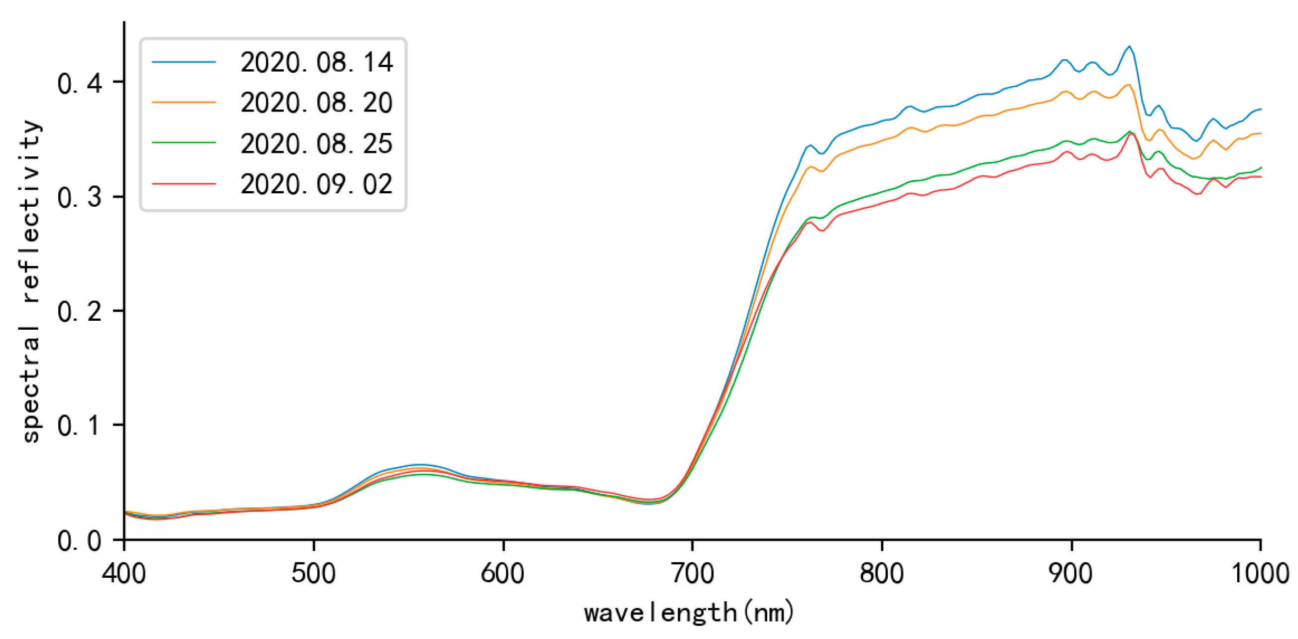
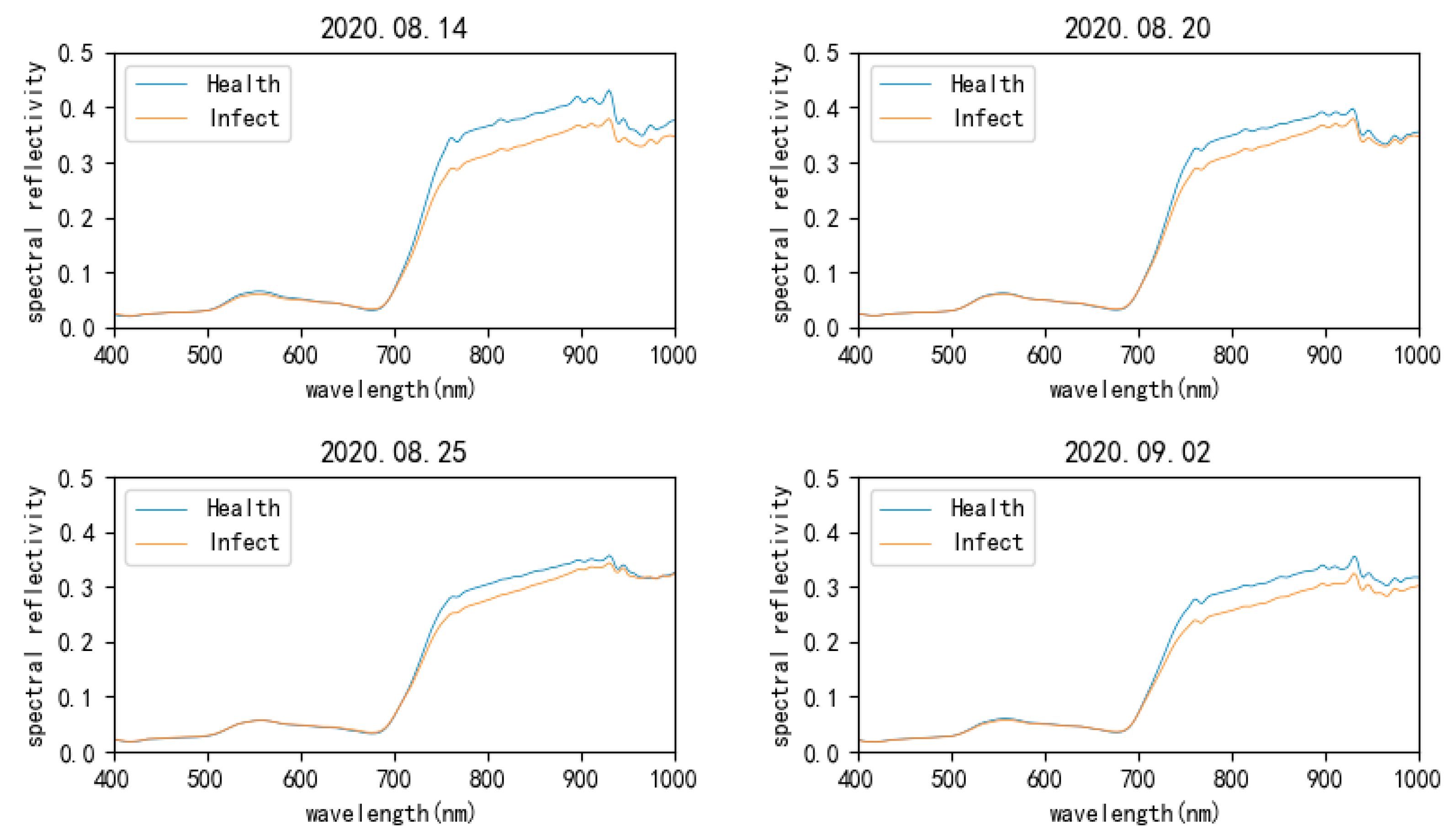
By comparison with Table 9 and Table 10, the Random Forest model has the highest prediction accuracy, but there are still nearly 14% wrong classifications. Misclassification can be divided into two categories: misidentification of healthy as infected and misidentification of infected as healthy. First, if health is wrongly identified as infected, recall (Equation (7)) can be used to evaluate it. Recall refers to the proportion of health data that is actually healthy among all the predicted health data. The greater the recall, the more health can be correctly predicted. The recall of optimal prediction accuracy of the random forest model was 92.17%, indicating that less than 8% of healthy samples were wrongly identified as infected. The main reason for this wrong prediction was the difference in rice growth. The spectral reflectance of rice infected with growth (see Figure 9), and the spectral reflectance of infected rice was less than that of healthy rice (see Figure 10) during the same period. Therefore, the spectral reflectance of healthy rice with a fast growth rate is lower than that of other healthy rice, and it is more similar to the spectral reflectance of infected rice, so it is easier to be wrongly identified as infected rice. Secondly, the infected rice was misidentified as healthy, and the main reason was that the spectral reflectance of the newly infected rice was similar to that of the healthy rice, so it was easy to be identified as healthy. In view of the above two situations, it is not easy to solve the problem that health is wrongly identified as infected, but if the disease is predicted as healthy, the difference between infected rice and healthy rice can be expanded through data processing methods such as integration or finding relevant spectral characteristic parameters to improve the prediction accuracy of the mode, which is a direction of future research. In addition, the spectral reflectance of healthy rice was greater than that of diseased rice, which was consistent with the conclusion of previous studies [46].

According to the prediction results in Figure 8, it can be seen that at the beginning, a few patches of regional rice were infected with rice false smut, while only small areas were infected in other areas, which conforms to the law of rice false smut infection under natural conditions. By comparing the predicted results at four different time points, we can see that the infection rate of rice false smut to the surrounding healthy rice in the early stage was slow, then the infection rate of rice false smut was accelerated and finally, the rice was widely infected with rice false smut. Therefore, for the monitoring of rice false smut, the earlier the detection time, the better the control effectively and the early heading stage of rice is an important time point for the control of rice false smut.

Although this study gained relatively accurate rice false smut data through field data measurement, it does not mean that there was no interference from other diseases and pests that could not be visually identified at the initial stage, especially when overlapping with the spectral reflection curve of rice false smut infection. In the meantime, there is room for improvement in the distortion of measurement data caused by rice position migration. Therefore, there are still some limitations to our study.

5. Conclusions

In this paper, we discuss how to accurately identify rice false smut by optimizing the band of UAV hyperspectral image to achieve data noise reduction in hyperspectral image. By using RF and GBDT models to test the effectiveness of three different optimization methods, GA, PCC and ISIC, an effective method to select the hyperspectral characteristic bands was obtained and a model method for high-precision monitoring of rice false smut. The conclusion is as shown below:

(1)

The method of hyperspectral characteristic bands selecting based on genetic algorithm, correlation coefficient method and Instability Index between Classes is an effective band selection method. It can effectively reduce the data dimension (27.78% of bands can be further eliminated in this paper) and reduce the amount of data while ensuring the monitoring accuracy of the model.

(2)

The selection of bands with strong correlation will reduce the model monitoring accuracy.

(3)

The difference of spectral characteristics between diseased and healthy rice is a useful information for monitoring rice false smut.

(4)

The sensitive bands of rice false smut surveillance ranged between 698–800 nm and 974–997 nm.

(5)

Both RF model and GBDT model can effectively extract the affected areas of rice false smut. The RF model has higher accuracy and the GBDT model has higher potential to improve accuracy.

(6)

The early heading stage is an important time point for controlling rice false smut.

Although the consequences of this study are encouraging, there are some limitations to this study that should be addressed in future studies. For example, rice can be divided into early ripening and late ripening and there are also different varieties. The method adopted in this paper should be tested in different regions, growth cycles and varieties of rice. In addition, since rice reflectance is used in this study to monitor rice false smut, it may be affected by the background (such as soil and weeds), so the subsequent research shall consider removing soil and weeds to improve the accuracy of rice false smut monitoring.

References

1. Yang, N.; Chang, K.; Dong, S.; Tang, J.; Wang, A.; Huang, R.; Jia, Y. Rapid image detection and recognition of rice false smut based on mobile smart devices with anti-light features from cloud database. Biosyst. Eng. 2022, 218, 229–244. [Google Scholar] [CrossRef]
2. Sharma, R.; Kukreja, V. Rice diseases detection using Convolutional Neural Networks: A Survey. In Proceedings of the 2021 International Conference on Advance Computing and Innovative Technologies in Engineering (ICACITE), Greater Noida, India, 4–5 March 2021; pp. 995–1001. [Google Scholar] [CrossRef]
3. Su, J.; Liu, C.; Coombes, M.; Hu, X.; Wang, C.; Xu, X.; Li, Q.; Guo, L.; Chen, W.-H. Wheat yellow rust monitoring by learning from multispectral UAV aerial imagery. Comput. Electron. Agric. 2018, 155, 157–166. [Google Scholar] [CrossRef]
4. Yuan, L.; Huang, Y.; Loraamm, R.W.; Nie, C.; Wang, J.; Zhang, J. Spectral analysis of winter wheat leaves for detection and differentiation of diseases and insects. Field Crops Res. 2014, 156, 199–207. [Google Scholar] [CrossRef] [Green Version]
5. Li, Y.; Shi, J.; Xiang, Z.; Hu, R.; Shi, S.; Peng, T.; Liu, D.; Huang, T. Analysis of the Resistance to Rice Blast and False Smut of 18 Varieties of Hybrid Rice in Sichuan Province, China. Int. J. Agric. Biol. 2017, 19, 880–886. [Google Scholar] [CrossRef]
6. Nessa, B.; Salam, M.U.; Haque, A.M.; Biswas, J.K.; Kabir, M.S.; MacLeod, W.J.; D’Antuono, M.; Barman, H.N.; Latif, M.A.; Galloway, J. Spatial pattern of natural spread of Rice False Smut (Ustilaginoidea virens) disease in fields. Am. J. Agric. Biol. Sci. 2015, 10, 63–73. [Google Scholar] [CrossRef] [Green Version]
7. Wang, W.-M.; Fan, J.; Jeyakumar, J.M.J. Rice false smut: An increasing threat to grain yield and quality. In Protecting Rice Grains in the Post-Genomic Era; IntechOpen: London, UK, 2019; pp. 89–108. [Google Scholar] [CrossRef] [Green Version]
8. Liu, C.; Xu, C.; Liu, S.; Xu, D.; Yu, X. Study on identification of Rice False Smut based on CNN in natural environment. In Proceedings of the 2017 10th International Congress on Image and Signal Processing, BioMedical Engineering and Informatics (CISP-BMEI), Shanghai, China, 14–16 October 2017; pp. 1–5. [Google Scholar]
9. Prakobsub, K.; Ashizawa, T. Intercellular invasion of rice roots at the seedling stage by the rice false smut pathogen, Villosiclava virens. J. Gen. Plant Pathol. 2017, 83, 358–361. [Google Scholar] [CrossRef] [Green Version]
10. Andargie, M.; Congyi, Z.; Yun, Y.; Li, J. Identification and evaluation of potential bio-control fungal endophytes against Ustilagonoidea virens on rice plants. World J. Microbiol. Biotechnol. 2017, 33, 120. [Google Scholar] [CrossRef] [PubMed]
11. An, G.; Xing, M.; He, B.; Kang, H.; Shang, J.; Liao, C.; Huang, X.; Zhang, H. Extraction of Areas of Rice False Smut Infection Using UAV Hyperspectral Data. Remote Sens. 2021, 13, 3185. [Google Scholar] [CrossRef]
12. Zhang, N.; Yang, G.; Pan, Y.; Yang, X.; Chen, L.; Zhao, C. A review of advanced technologies and development for hyperspectral-based plant disease detection in the past three decades. Remote Sens. 2020, 12, 3188. [Google Scholar] [CrossRef]
13. Chen, L.; Xing, M.; He, B.; Wang, J.; Xu, M. Estimating Soil Moisture Over Winter Wheat Fields During Growing Season Using Machine-Learning Methods. IEEE J. Sel. Top. Appl. Earth Obs. Remote Sens. 2021, 14, 3706–3718. [Google Scholar] [CrossRef]
14. Xing, M.; Chen, L.; Wang, J.; Shang, J.; Huang, X. Soil moisture retrieval using SAR backscattering ratio method during the crop growing season. Remote Sens. 2022, 14, 3210. [Google Scholar] [CrossRef]
15. Guofeng, Y.; Yong, H.; Xuping, F.; Xiyao, L.; Jinnuo, Z.; Zeyu, Y. Methods and New Research Progress of Remote Sensing Monitoring of Crop Disease and Pest Stress Using Unmanned Aerial Vehicle. Smart Agric. 2022, 4, 1–16. [Google Scholar] [CrossRef]
16. Weiss, M.; Jacob, F.; Duveiller, G. Remote sensing for agricultural applications: A meta-review. Remote Sens. Environ. 2020, 236, 111402. [Google Scholar] [CrossRef]
17. Zhengwei, Y.; Wen-bin, W.; Liping, D.; Berk, Ü. Remote sensing for agricultural applications. J. Integr. Agric. 2017, 16, 239–241. [Google Scholar] [CrossRef]
18. Yang, J.; Xing, M.; Tan, Q.; Shang, J.; Song, Y.; Ni, X.; Wang, J.; Xu, M. Estimating Effective Leaf Area Index of Winter Wheat Based on UAV Point Cloud Data. Drones 2023, 7, 299. [Google Scholar] [CrossRef]
19. Calou, V.B.C.; dos Santos Teixeira, A.; Moreira, L.C.J.; Lima, C.S.; de Oliveira, J.B.; de Oliveira, M.R.R. The use of UAVs in monitoring yellow sigatoka in banana. Biosyst. Eng. 2020, 193, 115–125. [Google Scholar] [CrossRef]
20. Su, J.; Liu, C.; Hu, X.; Xu, X.; Guo, L.; Chen, W.-H. Spatio-temporal monitoring of wheat yellow rust using UAV multispectral imagery. Comput. Electron. Agric. 2019, 167, 105035. [Google Scholar] [CrossRef]
21. Lu, J.; Zhou, M.; Gao, Y.; Jiang, H. Using hyperspectral imaging to discriminate yellow leaf curl disease in tomato leaves. Precis. Agric. 2018, 19, 379–394. [Google Scholar] [CrossRef]
22. Adam, E.; Deng, H.; Odindi, J.; Abdel-Rahman, E.M.; Mutanga, O. Detecting the early stage of phaeosphaeria leaf spot infestations in maize crop using in situ hyperspectral data and guided regularized random forest algorithm. J. Spectrosc. 2017, 2017, 2314–4920. [Google Scholar] [CrossRef] [Green Version]
23. Nagasubramanian, K.; Jones, S.; Sarkar, S.; Singh, A.K.; Singh, A.; Ganapathysubramanian, B. Hyperspectral band selection using genetic algorithm and support vector machines for early identification of charcoal rot disease in soybean stems. Plant Methods 2018, 14, 86. [Google Scholar] [CrossRef] [Green Version]
24. Zhao, Y.; Xu, X.; Liu, F.; He, Y. A novel hyperspectral waveband selection algorithm for insect attack detection. Trans. ASABE 2012, 55, 281–291. [Google Scholar] [CrossRef]
25. Jin, X.; Jie, L.; Wang, S.; Qi, H.J.; Li, S.W. Classifying wheat hyperspectral pixels of healthy heads and Fusarium head blight disease using a deep neural network in the wild field. Remote Sens. 2018, 10, 395. [Google Scholar] [CrossRef] [Green Version]
26. Qiao, T.; Lv, C.; Xiao, W. Hyperspectral prediction model of soil texture based on genetic algorithm. Chin. J. Soil Sci. 2018, 49, 773–778. (In Chinese) [Google Scholar] [CrossRef]
27. Liu, Z.-Y.; Wu, H.-F.; Huang, J.-F. Application of neural networks to discriminate fungal infection levels in rice panicles using hyperspectral reflectance and principal components analysis. Comput. Electron. Agric. 2010, 72, 99–106. [Google Scholar] [CrossRef]
28. Knauer, U.; Matros, A.; Petrovic, T.; Zanker, T.; Scott, E.S.; Seiffert, U. Improved classification accuracy of powdery mildew infection levels of wine grapes by spatial-spectral analysis of hyperspectral images. Plant Methods 2017, 13, 47. [Google Scholar] [CrossRef] [Green Version]
29. Press, W.H.; Teukolsky, S.A. Savitzky-Golay smoothing filters. Comput. Phys. 1990, 4, 669–672. [Google Scholar] [CrossRef]
30. Savitzky, A.; Golay, M.J. Smoothing and differentiation of data by simplified least squares procedures. Anal. Chem. 1964, 36, 1627–1639. [Google Scholar] [CrossRef]
31. Katoch, S.; Chauhan, S.S.; Kumar, V. A review on genetic algorithm: Past, present, and future. Multimed. Tools Appl. 2021, 80, 8091–8126. [Google Scholar] [CrossRef] [PubMed]
32. Rowe; Jonathan, E. Genetic algorithm theory. In Proceedings of the Conference Companion on Genetic & Evolutionary Computation, Dublin, Ireland, 12–16 July 2011; p. 1029. [Google Scholar]
33. Benesty, J.; Chen, J.; Huang, Y.; Cohen, I. Pearson correlation coefficient. In Noise Reduction in Speech Processing; Springer: Berlin/Heidelberg, Germany, 2009; Volume 5, pp. 1–4. [Google Scholar]
34. Deng, J.; Deng, Y.; Cheong, K.H. Combining conflicting evidence based on Pearson correlation coefficient and weighted graph. Int. J. Intell. Syst. 2021, 36, 7443–7460. [Google Scholar] [CrossRef]
35. Xue, X.; Zhou, J. A hybrid fault diagnosis approach based on mixed-domain state features for rotating machinery. ISA Trans. 2017, 66, 284–295. [Google Scholar] [CrossRef]
36. Akoglu, H. User’s guide to correlation coefficients. Turk. J. Emerg. Med. 2018, 18, 91–93. [Google Scholar] [CrossRef]
37. Somers, B.; Delalieux, S.; Stuckens, J.; Verstraeten, W.; Coppin, P. A weighted linear spectral mixture analysis approach to address endmember variability in agricultural production systems. Int. J. Remote Sens. 2009, 30, 139–147. [Google Scholar] [CrossRef]
38. Breiman, L. Random forests. Mach. Learn. 2001, 45, 5–32. [Google Scholar] [CrossRef] [Green Version]
39. Li, X. Application of random forest model in classification and regression analysis. Chin. J. Appl. Entomol. 2013, 4, 1190–1197. [Google Scholar]
40. Zhang, Z.; Jung, C. GBDT-MO: Gradient-Boosted Decision Trees for Multiple Outputs. IEEE Trans. Neural Netw. Learn. Syst. 2020, 32, 3156–3167. [Google Scholar] [CrossRef]
41. Luque, A.; Carrasco, A.; Martín, A.; de Las Heras, A. The impact of class imbalance in classification performance metrics based on the binary confusion matrix. Pattern Recognit. 2019, 91, 216–231. [Google Scholar] [CrossRef]
42. An, G.; Xing, M.; He, B.; Liao, C.; Huang, X.; Shang, J.; Kang, H. Using machine learning for estimating rice chlorophyll content from in situ hyperspectral data. Remote Sens. 2020, 12, 3104. [Google Scholar] [CrossRef]
43. Liu, Z.-y.; Shi, J.-j.; Zhang, L.-w.; Huang, J.-f. Discrimination of rice panicles by hyperspectral reflectance data based on principal component analysis and support vector classification. J. Zhejiang Univ. Sci. B 2010, 11, 71–78. [Google Scholar] [CrossRef] [PubMed] [Green Version]
44. Liu, X.-D.; Sun, Q.-H. Early assessment of the yield loss in rice due to the brown planthopper using a hyperspectral remote sensing method. Int. J. Pest Manag. 2016, 62, 205–213. [Google Scholar] [CrossRef]
45. Liu, Z.-Y.; Qi, J.-G.; Wang, N.-N.; Zhu, Z.-R.; Luo, J.; Liu, L.-J.; Tang, J.; Cheng, J.-A. Hyperspectral discrimination of foliar biotic damages in rice using principal component analysis and probabilistic neural network. Precis. Agric. 2018, 19, 973–991. [Google Scholar] [CrossRef]
46. Chen, F.; Zhang, Y.; Zhang, J.; Liu, L.; Wu, K. Rice false smut detection and prescription map generation in a complex planting environment, with mixed methods, based on near earth remote sensing. Remote Sens. 2022, 14, 945. [Google Scholar] [CrossRef]
Figure 1. DJI Matric 600 Pro, Nano-HyperSpec®, Ruyin Ronin-MX.
Remotesensing 15 02961 g001
Figure 2. Information map of the geographical location of the study area and the incidence of rice false smut. (a) Geographical location of the pilot area; (b) Top view of the test plot; (c) Sampling area selection distribution map.
Remotesensing 15 02961 g002
Figure 3. Comparison of rice spectral data before and after S–G filtering.
Remotesensing 15 02961 g003
Figure 4. Band selection workflow.
Remotesensing 15 02961 g004
Figure 5. Band selection by genetic algorithm. (a) Band selection histogram of genetic algorithm; (b) Band selection results by genetic algorithm.
Remotesensing 15 02961 g005
Figure 6. The number on the upper and left side is the wavelength (nm) of the selected characteristic band of genetic algorithm, the color in the figure is the size of the correlation coefficient between each band vector and the square grid is the value of the correlation coefficient of the band vector.
Remotesensing 15 02961 g006
Figure 7. Genetic algorithm screening of the Instability Index between Classes of each feature band. The dashed line is the selected threshold.
Remotesensing 15 02961 g007
Figure 8. Temporal and spatial distribution map of rice false smut occurrence information in the study area: (a) 14 August 2020; (b) 20 August 2020; (c) 25 August 2020; (d) 2 September 2020.
Remotesensing 15 02961 g008
Figure 9. Spectral reflectance changes of healthy rice at four different dates.
Remotesensing 15 02961 g009
Figure 10. Comparison of spectral reflectance between healthy rice and diseased rice on four different dates.
Remotesensing 15 02961 g010