Review

Remote Sensing and Data Analyses on Planetary Topography

1
Department of Geoinformatics, University of Seoul, Seoulsiripdaero 163, Dongdaemum-gu, Seoul 02504, Republic of Korea
2
Department of Land Economics, National Chengchi University, No. 64, Sec. 2, Zhinan Rd., Wenshan Dist., Taipei City 116, Taiwan
3
Institute of Geodesy and Geoinformation Science, Technische Universität Berlin, Kaiserin-Augusta-Allee 104-106, 10553 Berlin, Germany
*
Author to whom correspondence should be addressed.
Remote Sens. 2023, 15(12), 2954; https://doi.org/10.3390/rs15122954
Submission received: 29 March 2023 / Revised: 25 May 2023 / Accepted: 31 May 2023 / Published: 6 June 2023
(This article belongs to the Special Issue Planetary Exploration Using Remote Sensing)

Abstract

:
Planetary mapping product established by topographic remote sensing is one of the most significant achievements of contemporary technology. Modern planetary remote sensing technology now measures the topography of familiar solid planets/satellites such as Mars and the Moon with sub-meter precision, and its applications extend to the Kuiper Belt of the Solar System. However, due to a lack of fundamental knowledge of planetary remote sensing technology, the general public and even the scientific community often misunderstand these astounding accomplishments. Because of this technical gap, the information that reaches the public is sometimes misleading and makes it difficult for the scientific community to effectively respond to and address this misinformation. Furthermore, the potential for incorrect interpretation of the scientific analysis might increase as planetary research itself increasingly relies on publicly accessible tools and data without a sufficient understanding of the underlying technology. This review intends to provide the research community and personnel involved in planetary geologic and geomorphic studies with the technical foundation of planetary topographic remote sensing. To achieve this, we reviewed the scientific results established over centuries for the topography of each planet/satellite in the Solar System and concisely presented their technical bases. To bridge the interdisciplinary gap in planetary science research, a special emphasis was placed on providing photogrammetric techniques, a key component of remote sensing of planetary topographic remote sensing.

1. Introduction

It is believed that planetary mapping began with the first observation of the Moon using a telescope. That implies that the history of remote sensing applications on planetary topography is even longer than terrestrial remote sensing. From 1600 to 1800, many observers tried to depict the planetary surface by sketching maps based on the telescope image. The first one produced for positional measurements with a coordinate system was Tobius Mayer’s Moon sketch in 1775 [1].
In the 20th century, Kuiper et al. (1960, cited in Greeley et al. [2]) compiled telescopic images with several different illumination conditions and produced a lunar atlas. It is considered to be the first extraterrestrial cartographic map. In the 1960s, the U.S. Air Force Chart and Information Center (ACIS) and the National Aeronautics and Space Administration (NASA) started to introduce modern mapping technologies like image processing and stereo photogrammetry for planetary mapping [3]. Additionally, the Lunar and Planetary Laboratory established by the University of Arizona applied geodetic control to planetary map construction in 1960. Then the turning point came with the acquisition of planetary images by the spacecraft camera. The true milestone of remote sensing on the planetary surface was set by Luna 3 of the Soviet Union, which delivered the backside photo of the Moon that was never revealed to a human being. Twenty-nine images were transmitted to the terrestrial ground station [4].
From the late 1960s, the resolution of planetary images increased to several hundred meters from a few kilometers. Electronically transferred imaging on the Moon, Mars, and Venus stimulated the development of the digital image processing method. Thus, the contemporary electro-optical (EO) technical bases are somehow rooted in planetary remote sensing. On the technical side, the significant milestone in planetary remote sensing was the Apollo series, equipped with modern mapping technology like stereoscopic cameras on Apollo 11 and 12, stereo panoramic cameras, and laser altimeters for 3D control point assignment in Apollo 15, 16, and 17 [5]. It was the first geodetic control over extraterrestrial remote sensing based on spacecraft imagery. The scope of planetary remote sensing has been continuously extended. From 1973, the other planets, Mercury, Venus, and Mars, were observed by several successful missions. In 1978, Pioneer Venus performed radar altimetry observations and synthetic aperture radar (SAR) measurements of the Venusian surface. Based on such data, a 1:50,000,000 map, the first topographic product by direct measurement of an active sensor, was produced [6,7]. The outer planets, Jovian, Saturnian, and Uranian systems, were observed by Voyager 1 and 2, and their airbrush maps were constructed by a digital mosaic technique at several hundred-meter resolution.
The Clementine and Mars Global Surveyor (MGS) in the 1990s were the first spacecraft equipped with high-resolution laser altimeters (1 m in vertically and 400 m in planimetrically), which directly measured global 3-D topographical data over the lunar and Martian surfaces [8,9]. In a densely atmospheric planet such as Venus, the medium resolution (≈14 km) of a radar altimeter was employed for the construction of the digital elevation model (DEM) by the Magellan mission in 1992 [10]. In the 21st century, planetary mapping missions with higher resolution and wider range were implemented, including Cassini [11,12], Mars Express [13], and even the Pluto and Kuiper belt missions by New Horizons [14]. Now, the missions by new peers such as Chandrayaan [15,16], Chang’e [17,18,19], Tianwen series [20], and Emirates Mars mission [21] have been newly joined for the construction of topographic data. Since then, with properly rectified images and other sources of topographic data applied by improved photogrammetric techniques, the outcomes of planetary topographic remote sensing have been available for scientific research as well as public interactions.
Despite such remarkable achievements in remote sensing techniques for planetary surface reconstruction, there is still a lack of understanding of discipline-specific remote sensing processes. Although the technical basis of planetary remote sensing is similar to mainstream remote sensing techniques, inaccurate or ambiguous information is disseminated to the public and the remote sensing research community through scientific news and even some academic publications. As a result, even today, these misconceptions affect education, research, and project planning related to the field.
This review aims to address the existing knowledge gap and promote a comprehensive understanding of planetary topographic remote sensing. It emphasizes the need to overcome misconceptions and inaccurate information that has been disseminated to the public and the remote sensing research community. The objective of providing a fundamental comprehension of this field is to establish a solid foundation for open and unbiased academic discourse in education, research, and project planning.
As follows, all major achievements of planetary topographic remote sensing are briefly reviewed in Section 2. The essential technical bases for such achievements are then discussed in Section 3. The applications and compilation of planetary topographic remote sensing data are discussed in Section 4. The proposition for future progress was summarized in Section 5 and the conclusions that follows.

2. Review of Planetary Topography Mapping

2.1. Moon

The first spacecraft image was taken by Russia’s Luna 3 in 1959. In the 1960s, most of the spacecraft in the U.S. Ranger project were successfully launched, and ACIS released maps of the Moon at various scales based on Ranger images. To support further studies of the Moon, automated mapping, stereo panoramic cameras, and laser altimeters for 3D control point assignment were developed and carried out on the Apollo 15, 16, and 17 missions [22].
The next highlight of lunar surface mapping was achieved through the Clementine project, launched in 1994 [23]. On this mission, a series of camera systems, including two Star Tracker (ST) cameras, an ultraviolet-visible (UVVIS) camera, a near-infrared (NIR) camera, a long-wave infrared (LWIR) camera and a high-resolution (HIRES) camera, recording multiple spectral reflections in various spatial resolution (ranging from 30 to 1150 m per pixel at an altitude of 425 km) were carried. In addition, a laser image detection and ranging (LIDAR) system capable of measuring the distance from the spacecraft to the lunar surface was installed onboard to produce 3D topographic products [24]. Combing the data collected from UVVIS, NIR, LWIR, HIRES, and LIDAR, the lunar surface was covered completely during the two-month systematic mapping phase of the mission [25]. The most commonly used product is the lunar mosaic basemap generated by the United States Geological Survey (USGS) [8]. Of these, a total of approximately 43,000 UVVIS images were radiometrically calibrated, photometrically corrected, geodetically controlled [26], and projected onto a spherical model of the Moon to create a global mosaic at a 100 m resolution. In order to improve accuracy, subsequent upgrades to the basemap were made based on improvements in the lunar geodetic control network and the availability of detailed 3D shape models (refer to Section 3.4).
In the 21st century, the first notable lunar mapping mission was the Small Mission for Advanced Technology Research One (SMART-1), launched in 2003, the first European-sanctioned lunar mission [27]. In SMART-1, three remote sensing instruments are used for various mapping purposes: (1) The global X-ray mapping spectrometer (D-CIXS) with solar X-ray monitor (XSM) was developed to map potential lunar resources, such as Mg, Si, Ca, Fe, and Al; (2) Based on the hyperspectral specification, the near-infrared mapping spectrometer SIR aimed to map the mineral composition of the entire lunar surface with a maximum spatial resolution of 300 m [28]; (3) The Advanced Moon Imaging Experiment (AMIE) was used to acquire high-spatial resolution (up to 30 m) color images over selected local areas [29]. High-resolution AMIE images could be used to investigate geomorphologic features. Although a planimetric offset in the order of km was observed when compared with the Clementine basemap [30], the AMIE images were applied to support a scientific interpretation of the lunar south pole [31,32].
Following SMART-1, the space agencies of some Asian countries successively launched three lunar exploration missions in 2007 and 2008, the Selenological and Engineering Explorer (SELENE) [33], Chang’e 1 [19] and Chandrayaan-1 SAR [34] respectively developed by the Japan Aerospace Exploration Agency (JAXA), the China National Space Administration (CNSA), and the Indian Space Research Organisation (ISRO). The remote sensing instruments carried onboard were similar to the payloads of the Clementine and SMART-1 missions. They could be categorized into resource mapping or topographic analysis sensors based on the applications. As the latter equipment is the focus of this paper, we list the sensors and related specifications in Table 1 [16,33,35]. From the perspective of hardware design, the stereo camera system and laser altimeter have obviously become the standard equipment package for the implementation of lunar topographic exploration. The spatial resolution of the camera system could achieve 10 m per pixel, whereas the elevation resolution of the laser ranger normally ranged between 5 and 10 m.
A high-resolution lunar topographic model was created using data from the laser altimeter (LALT), with a global map having a spatial resolution finer than 0.5 degree [37]. Later, a terrain model with a spatial resolution of 0.25° and an absolute vertical accuracy of about 31 m was generated based on over three million range measurements derived from the Chang’e-1 laser altimeter [43]. In addition to the improved accuracy, another feature of this model was the coverage over polar regions through intensive laser measurements. The SELENE laser altimeter observations were also processed to produce local DEMs to estimate the sunlit conditions [44] and hydrogen deposits [45] in polar regions. Furthermore, lunar north and south pole coverage by the lunar laser ranging instrument (LLRI) onboard Chandrayaan-1 was reported by Bhaskar et al. [46].
Shortly after the launch of India’s Chandrayaan-1, the Lunar Reconnaissance Orbiter (LRO) was successfully sent to the Moon [47]. As listed in Table 1, it is highlighted that the spatial resolution of the camera system carried onboard significantly improved to 0.5 m per pixel. Such advanced images demonstrating clear surface features have been successfully applied in high-resolution DEM production [48], landing site and traverse design [49], and feature exploration in and around lunar craters [50,51]. As for the LOLA experiment, it was reported that a global DEM with a resolution of 0.0625° (2 km) [52] was produced based on over 6.8 billion laser measurements [53]. After an adjustment conducted by Mazarico et al. [54], a 1/256° resolution global lunar DEM with an average accuracy better than 20 m in horizontal position and 1 m in vertical direction, is accessible in the NASA Planetary Data System (PDS) [42] (see Figure 1).
Relying on the successful development experience and scientific achievements obtained in these missions, CNSA launched Chang’e-2, 3, 4, and 5 in 2010, 2013, 2018, and 2020, respectively [17,18,55,56]. ISRO launched Chandrayaan-2 (2019) [15] to continue their exploration of the Moon. Looking back at past developments, first, it is worth noting that offsets between the various lunar DEMs were noted as many terrain products were already available. Since using multiple topographic products simultaneously would lead to misinterpretation, solutions such as surface matching technology were implemented to reduce the ~170 m vertical offset between Chang’e-1 laser altimeter (LAM) and SELENE LALT to ~20 m, while eliminating about 70 m of offset between LRO LOLA and SELENE LALT [57]. Second, an integration of multiple topographic data sets was also developed to extract information. For example, by integrating the imagery and laser altimeter data derived from the Chang’e-1 mission, an updated local DEM was further generated over areas of the Apollo 15 and 16 landing sites [58]. Barker et al. [59] employed the LOLA and SELENE Terrain camera (TC) data to improve the performance of lunar DEM. Kokhanov et al. [60] mapped potential lunar landing zones using LRO orthorectified narrow Angle camera (NAC) images and SELENE DEM. The ShadowCam [61] aboard the Korean Pathfinder Lunar Orbiter (KPLO), which entered polar orbit in 2023, is the first optical sensor capable of observing the permanent shadowed regions (PRRs) of the Moon’s poles to search for signs of frozen water.

2.2. Mars

Following Huygens’ first sketches of Martian surface features in 1636 and 1640, Schiaparelli produced the first comprehensive map with orientation and georeferencing in 1877 using the Mercator projection [62]. In 1950, the IAU (International Astronomical Union) compiled L.C. Slipher and other telescope observation data at Lowell Observatory, and published the first general map of Mars in 1960 [63]. The actual topographic image products were not recorded until the first successful Martian spacecraft mission, Mariner 4, in 1965 [64]. The images captured by the Mariner series have a resolution of 3 km in the best case. New techniques in digital image processing have made it possible to publish improved images that reveal previously unseen details of surface features [65]. During their flyby missions in 1969, Mariners 6 and 7 captured wide-angle images of the entire surface and close-up images of 20% of the Martian surface [66].
In 1971, Mariner 9 achieved the first milestone in mapping the surface of Mars. For the first time, these data became the basis for mapping entire planets from space. This was conducted by the USGS in Flagstaff, the main U.S. planetary mapping agency, which released 1:250,000 and 1:500,000 maps [67]. In 1976, the successful missions of the Viking 1 and Viking 2 orbiters became the primary data source for Mars mapping, providing 55,000 images with resolutions ranging from 7 m to 1000 m [68,69]. One of the most important results was that the Viking Landers provided decent geodetic landmarks on Mars, as their position on the Martian surface could be determined by radio ranging with an accuracy of a few hundred meters. Various attempts to identify them in Viking orbiter images or images from other missions have been made [70] and processed to establish the primary control point on the Martian surface with reliable accuracy. From 1976 to 1980, two Viking orbiters equipped with two identical Vidicon cameras, which were called the Vision Imaging System, VIS, orbited Mars [71]. Each system consisted of a telescope, a slow scan vidicon, a filter wheel, and electronic equipment. Mars Mosaicked Digital Image Models (MDIMs) were produced from original Viking orbiter images at 1/16, 1/64, and 1/256 degree resolutions through radiometric, geometric, photometric, and controlled mosaic [72,73].
The Mars Orbiter Laser Altimeter (MOLA) was the first laser altimeter system for global Mars topographical mapping. The coverage ranges from the northern polar ice cap to the equator in Science Phase 1 and the entire Martian surface in the mapping phase [74]. As listed in Table 2, the major components of MOLA are a diode-pumped Nd:YAG laser transmitter, a 0.5 m diameter telescope, and a silicon avalanche photodiode detector [75]. During all observation phases, MOLA derived topographical measurements of Mars through the continuous collection of laser reflection. The laser footprint size is approximately 120 m, and the footprint spacing is 300 m along track. The measurement reached 1.5 m vertical resolution without orbit and pointing error corrections [76]. MOLA gathered enough data spots to allow the establishment of a global DEM with 1/256 by 1/256 degree grid (231.6 m at the equator), which is referenced to Mars’ center-of-mass with an absolute accuracy of approximately 30 m and included surface reflectivity (as shown in Figure 2) [77].
MOLA and Mars orbiter camera (MOC) equipped with MGS has made a major leap forward in mapping Mars. MOC was based on the “pushbroom” technique that acquires data one row at a time along the spacecraft orbits [78]. Thus, the coverage of the wide-angle (WA) camera included the full Martian surface and was able to be controlled by MOLA tracks. The narrow-angle (NA) channels of MOC acquired high-resolution images and revealed detailed geological features of the Martian surface [9]. Moreover, the employment of photogrammetric routines enabled the detailed 3D mapping of interesting geological processes [79,80,81]. Note that this is actually the first case of high-resolution 3D mapping of the surface of a planet other than the Moon. Studies of impact structure and sedimentary processes, polar processes and deposits, volcanism, and other geologic/geomorphic processes benefit from such high-resolution data. The standard error of the control network used for geocoding was known to be only on the order of 5 km. However, it was used as a base map for topographical mapping and MDIM 2.1 was released, which was orthorectified using the MOLA DEM and with better control accuracy [82].
The MARS Express, the first planetary mission of the European Space Agency (ESA), was launched in June 2003 and entered an elliptical orbit on 25 December 2003 [13]. The high resolution stereo camera (HRSC), which is the main optical instrument of MARS Express, began its operational phase in early 2004 and is expected to have a mission lifetime of at least one Martian year, but it is still performing its mission [83]. Its major goal is to cover global Mars in high-resolution stereo color images based on high-precision geodetic control [84]. The instrument is a pushbroom scanner that can capture high-resolution imaging data of a specific area with a near-simultaneous acquisition, featuring along-track triple stereo, four colors, and five distinct phase angles. The secondary optical instrument, the super-resolution camera (SRC), is a framing device to yield narrow-angle images with a resolution of a few meters, but it was unusable in most cases due to camera calibration issues. During its nominal mission lifetime of 2 years, HRSC is projected to cover 50% of the Martian surface at a resolution of 15 m in its images [83]. In its first 1000 orbits, HRSC acquired about 10% of the Martian surface. Nadir images with better than 250 m/pixel resolution covering regional areas [85] are highly useful for studying time-varying features like clouds, polar cap edges, and wind streaks, as well as for obtaining stereoscopic coverage of areas of geological interest [86]. Additionally, the HRSC’s imaging capabilities allow for capturing limb images with an along-track resolution better than 1.5 km. The wide-angle cameras have color filters, which enable capturing color images of the surface and atmosphere. These images are useful in distinguishing between clouds and the ground and clouds of different compositions.
The High Resolution Imaging Science Experiment (HiRISE) and context camera (CTX), which are installed on the Mars Reconnaissance Orbiter (MRO), were designed to carry out tasks similar to those of the WA and NA of the MOC, with CTX covering a wider area and HiRISE’s detailed focus sub-meter resolution [87,88]. Compared to the 1–2 m resolution imaging provided by MOC NA images, the 40 cm GSD of HiRISE, together with stereo capability, opened up new horizons in planetary surface mapping. Instead of the 10-CCD structure design of HiRISE, stereo CTX with 6 m spatial resolution and stable imaging based on single-CCD geometry [88] was also highly effective for the mapping of the Martian surface [87,89]. Over the past decade, these two sensors have produced very valuable image products covering 1% and 99.1% of the surface of Mars, respectively (https://mars.nasa.gov/resources/8334/mars-global-coverage-by-context-camera-on-mro/, accessed on 28 March 2023). It should be noted that the real value of HiRISE and CTX imaging lies in their high-resolution stereo capabilities based on a high signal-to-noise ratio and stable gimbal control, which enable the construction of sub-meter and decadal-meter DEMs over major geological interests [90]. The mission of the colour and stereo surface imaging system (CaSSIS) on the ExoMars Trace Gas Orbiter was designed to perform a similar mission to the CTX, but with greater stereo capabilities, and was deployed in Mars orbit in 2018 [91]. The Indian Mars orbiter, Mangalyaan, which reached Mars orbit in 2014, provided a few images taken by the Mars colour camera (MCC) [92]. In both cases, the images and scientific results published so far remain limited. The Chinese Mars mission, Tianwen-1, completed the topographic mapping of the “Lover” landing site, which is not yet open to the public [20,93].

2.3. Venus/Mercury—Inner Planets

Although the orbital remote sensing of inner planets encounters difficulties due to navigation issues, the mapping of Mercury and Venus was still accomplished by several successful mapping projects.
In the case of Venus, the biggest challenge for topographic mapping is its dense atmosphere, which screens out the in-orbital optical imaging. Radar imaging and altimetry became the sole method used to construct the topography of Venus. In 1978, Pioneer Venus performed the first topographic mapping by radar altimetry and SAR [6,94]. Based on Pioneer Venus altimeter observations, a topographic map with a resolution of 20 km, the first topographic product by direct measuring of an active sensor over the planet’s surface, was constructed [6,7,95,96]. In addition, the imaging Radar of Pioneer Venus identified the detailed geological features on the Venusian surface, such as two continental scale highlands and one of the biggest volcanoes in the Solar System [96,97,98]. Note that the existence of such planet-scale geological features on Venus was recognized by the Arecibo Radio Telescope [99]. A follow-up Venus mission, Magellan in 1992 [10], was equipped with an improved radar altimeter and imaging mode [100], and produced the medium resolution (≈14 km) DEM for the whole Venus surface [7,101]. It revealed the details of Venusian tectonics [102], volcanoes [103], crater structures [104], channels, and valleys [105]. Employing the imaging mode of Magellan radar, the stereo topographic analyses on Venus’s surface have been conducted [106]. Up to now, the coverage by stereo interpretation using the Magellan radar image cover only a tiny fraction of the Venusian surface [107,108]. Therefore, altimetry DEM is the only data set for the study of Venus topography, together with a radar mosaic image in medium resolution.
The topographic mapping of Mercury performed better than the mapping of Venus, as the optical image and laser altimeter could cover the planet’s surface due to the absence of a dense atmosphere. However, until now, only two spacecrafts have ever reached the planet, that is, three flybys of the Mariner 10 and orbital observations of the Mercury Surface, Space Environment, Geochemistry and Ranging (MESSENGER). The first arrival of the imaging sensor equipped in Mariner 10 is dated to relatively early 1973 [109], and only a tiny fraction of images could be employed for the systematic stereo analysis [110]. Thus, a small portion of the surface was mapped before the arrival of MESSENGER. An interesting study of Mariner images was the application to surface photometric function analysis that became a standard method for interpreting the microscopic properties of planetary regolith, as shown in [111]. MESSENGER arrived in Mercury’s orbit in 2011 and remained there until April 2015 [112,113]. It provided a comprehensive laser altimetry topography of the northern hemisphere with 500 m resolution [114] and full optical stereo coverage, as shown in [115,116,117]. Becker et al. [118] utilized narrow angle camera (NAC) and wide angle camera (WAC) images from MESSENGER to generate a global set of DEMs with a grid size of 665 m/pixel. Preusker et al. [117] combined NAC and WAC images to create stereo DEMs with a resolution of 222 m/pixel, which encompass four quadrangles of Mercury’s surface. However, it is important to recognize that the actual horizontal resolution of these DEMs may reach up to approximately 4 km [119]. These DEMs helped to comprehensively identify the details of the geological structures on Mercury such as mega-scale basin [115], tectonic structures [120], and volcanoes [121]. The interesting thing about such mapping tasks is that they have been conducted with a similar approach to the Martian case. It means stereo products were geodetically controlled based on the Mercury laser altimeter (MLA) data [117] that covers from the equator to 86°N mainly. It is worth noting that MESSENGER was placed in a near-polar orbit that was highly elliptical, with a periapsis of approximately 200–400 km and an apoapsis ranging between 15,000 and 20,000 km. As a result, the spatial resolution of the images decreases and the density of laser footprints increases as they approach the north pole. The laser profiles do not extend south of 20°S due to a limitation in maximum ranging distance. The topographic products suffer from a severe inhomogeneity in terms of quality. Furthermore, the need to always point the heat shield towards the Sun means the MLA profiles were acquired off-nadir (up to 60°) in the noon-midnight orbits, significantly deteriorating their geolocation accuracy. As of the current writing, the BepiColombo mission’s Mercury Planetary Orbiter (MPO), which is jointly contributed by ESA and JAXA, is en route to Mercury. It is expected to achieve orbit around the planet by December 2025 [122]. The planned orbit is a less eccentric one (480 km × 1500 km) that will yield a uniform and global coverage of Mercury’s surface. The camera [123] and laser altimeter [124] onboard will update the topography observed by MESSENGER and assist in geologic, geophysical, geomorphologic, thermal, and spectroscopic applications employed to understand the evolution of Mercury. Surface mapping coverage over Mercury is comparable to that over the Moon and Mars [117]. However, MLA’s precision is much lower than that of MOLA. The RMS height residual at cross-overs can reach hundreds of meters, which is much higher than the few meters achieved by MOLA.

2.4. Asteroids and Comets

For the last decades, asteroids and comets have been positioned as low priorities in the planetary topographic mapping project. The Mariner 9 mission’s encounter with Phobos and Deimos is considered the first mission with an asteroid [125,126], assuming their origin as captured asteroids. Due to Martian sensors’ enhanced observation density, such as Viking [127], HRSC [128,129,130], CTX, and HiRISE [131], Phobos has been the most precisely mapped Solar System object with controlled topographic products [132,133]. The spacecraft sensor was first used for observing Galileo imaging in 243 Ida with up to 95% surface coverage and better than 1 km/pixel resolution [134,135] and Gaspra with 80% surface coverage and up to 54 m/pixel resolution [136,137]. Thus the shapes of Ida and Gaspra were mapped three-dimensionally [135,138] in the relatively early stage of outer Solar System exploration. Near Earth Asteroid Rendezvous–Shoemaker (NEAR Shoemaker) was the first explorer equipped with a laser range meter and optical sensor [139]. As the most significant object of exploration, the 433 Eros was fully covered by a laser range meter with around 1 km/pixel resolution and extracted many geophysical and topographic evolutions [140]. 253 Mathilde is the other object in NEAR Shoemaker’s mapping capability [141]. Hayabusa [142,143,144], Rosetta [145,146,147], and Chang’e-2 [148], which are all not oriented to the topography of the asteroid or even the asteroid itself, gained flyby chances and used their imaging functionality to cover 10 more asteroid surfaces. Hayabusa’s flyby to 25,143 Itokawa [143] and Hayabusa-2′s flyby to 162,173 Ryugu [149] mainly succeeded in topographic mapping together with their sample return and lander missions. The best detailed mappings of astride objects were conducted from the Dawn mission on 4 Vesta [150] and 1 Ceres [151], the two biggest astride dwarf planets. It should be noted that the images by Dawn mission were applied to the sophisticated block adjustment procedure and achieved well controlled topographic products such as DEM and orthoimages [142]. Although OSIRIS-Rex (Origins, Spectral Interpretation, Resource Identification, Security, Regolith Explorer) is a sample return mission, the mapping of Bennu was highly successful [152]. Up until now, the topographic mapping of the comet was only achieved by the Rosetta mission over 67P/Churyumov-Gerasimenko employing LIDAR and optical images [145,147,153]. Even though future asteroid missions will concentrate on sample return, core study, and body capture, there will still be ambitious plans with topographic mappings, such as Lucy [154,155] to Jupiter Trojan mission [154,155,156].

2.5. Satellites of Giant Planets

The solid satellites of outer giant planets such as Saturn, Jupiter, Uranus, and Neptune have been of interest in research society as their origins in comparison to the inner world have keys to understanding the Solar System. However, the geological and geomorphic aspects of this satellite remained unknown until the Pioneer 10 and 11 spacecrafts flew by Saturn and Jupiter in 1973 and 1975, respectively, and captured pass-by images of the Saturnian and Jovian satellites, particularly those of the Galilean satellites. [157,158]. Therefore, Voyagers 1 and 2 can be considered the first platforms, which took valuable remote sensing data on the topography of satellites orbiting giant planets [159,160,161]. Voyager 1 made the first Jupiter flyby in 1979 and made rough mapping on Galileo satellites, including Io volcanoes, using the Imaging Science System [160]. Saturn flyby in 1980 by Voyager 1 failed to contribute much to satellite mapping of Saturn due to the less contact with the target objects and the thick atmosphere of Titan, which was of prime interest [162]. Voyager 2 was more successful due to a closer flyby distance and better contact with the solid satellites of Uranus and Neptune [163,164]. Voyagers 1 and 2 sometimes encountered objects at a few 10 thousand km distances and formed some stereo observations between 1 and 2 images, as shown studies on Galileo satellites [165,166]. Thus, geodetic control on the images was feasible and led to initial mapping products [167].
The Galileo mission aimed to conduct high-resolution mapping of the Galileo satellite on Jupiter with far higher resolutions than the Voyager mission [168]. However, the partial failure of the deployment of a high gain antenna reduced the transmitted data set to 10% of the original observations [169]. Especially, Io and Europa mapping outcomes were mostly lost. Although some surface characteristics of Galileo satellites, such as details of Io’s volcanoes [170] and the icy crust of Europa [171], were observed with far better resolution, the potential to conduct systematic mapping of the Jovian system was missed. The mapping of Jovian satellites was hence postponed until the future arrival of new Jupiter orbiters.
The Saturnian system particularly has been noticed by its giant satellite Titan, which has a thick atmosphere. However, it also provided a limited data inventory to achieve sufficient scientific information, even with the achievements of Voyagers 1 and 2. Instead, the Cassini Mission should be noted as a highly successful case mapping the satellite/planet screened by the atmosphere [172]. Cassini imaging radar and altimeter dramatically increased discoveries on Titan [12], such as the fluvial methane system [173,174], aeolian geomorphologies [175], and potential tectonic activities [176]. USGS has achieved full orthorectification of Titan images by Cassini imaging radar [177,178]. In addition, endeavors to increase the coverage of digital topography employing radargrammetry [179], radar altimetry [180], and SARtopo [181] have been actively conducted and have produced valuable scientific information. Despite the efforts to construct a global topographic map of Titan, the available spatial resolutions of the map are still low, with a range of—1700 m [182]. Thus, it should be updated by future missions. The optical imaging utilizing the visible and infrared mapping spectrometer (VIMS) achieved precious mapping products such as orthoimage coverages and partial DEMs over other Saturn satellites such as Enceladus and Lapetus [183]. Note that the surface of satellites of Neptune and Uranus satellites had been only mapped by partial Voyage 2 imaging camera coverages of Voyage 2 imaging camera. Due to the better flyby distance (>100,000 km) in the case of Neptune’s satellite, they possess relatively good resolutions. However, the ranges are far from sufficient to form any mapping products.

2.6. Trans-Neptunian Object (TNO)

Up until now, the only space mission to successfully map the objects in the Kuiper Belt is New Horizons [184]. Since space telescopic observation extracted some albedo information in Pluto, the success of the New Horizons mission covering Pluto, Charon [185,186], and Arrokoth [187] extends our scope in planetary topographic mapping into the minor bodies of the outer Solar System. Topographic remote sensing of New Horizons only depends on the long range reconnaissance imager (LORRI) [188]. Despite the great success of topographic mapping, including stereo analysis, which led to a number of scientific discoveries [189], the published technical bases of topographic processing of LORRI are limited, especially regarding geodetic control. By the end of the encounter, 42% of Pluto’s surface has been mapped by stereo DEMs (90 to 1120 m resolution) and by orthoimage sets covering the major Pluto surfaces [190]. The Charon mission of New Horizons was also successful and achieved 40% of DEM coverage with 0.1–1.5 km resolution and northern hemisphere orthoimage coverage with 300 m resolution [189]. At the moment, the problem of the Pluto and Charon mission is that their geodetic controls only depend on the navigation data due to the absence of reference height planes or point measurements as in Mars, the Moon, and Venus.
Perhaps another mission to the Kuiper Belt is not likely to happen in the next decade. Thus, the mapping of Pluto and Charon will be limited to re-analyses of New Horizons data sets, maybe together with the potential contribution of new generation space telescopes.

3. Technical Point of Review

3.1. Optical Image and Stereo/Mono Analysis

The interpretation of planetary images for topographic data extraction mainly depends on the photogrammetric analysis, although there are some cases for applying photoclinometry, that is, shape from shading [191,192,193]. If multi-angle coverage of a certain area is available, the accuracy of photogrammetric analyses will be increased by the stereo analysis. In both stereo/mono photogrammetric analyses, the essential components are (1) sensor model for the employed optical sensor; (2) geodetic control information; (3) image matcher in the case of stereo analysis. In addition, registration points and the base height plane data are necessary if the manual/automated geodetic correction is applied, as stated in Section 3.4.
The rigorous camera model is the traditional system for the construction of a pixel’s physical relationship between the image and real-world coordinates. It is based on geometrical constraints, or, in other words, on sensor parameters, so that the “modeling” encompasses an overall workflow to estimate rigorous sensor parameters from the geometric relationship between the image and the planetary topography. The target of sensor modeling in planetary has been moved into the pushbroom sensor model from the framing camera; thus, the complexity of sensor modeling has increased. Therefore, the applications of the pushbroom sensor models are discussed in two approaches, that is, the conventional pushbroom model and the HRSC case.
The basic formula for the rigorous camera model is the collinearity equation:
x x 0 = f m 11 X X L + m 12 Y Y L + m 13 Z Z L m 31 X X L + m 32 Y Y L + m 33 Z Z L y y 0 = f m 21 X X L + m 22 Y Y L + m 23 Z Z L m 31 X X L + m 32 Y Y L + m 33 Z Z L
where
M = m 11 m 12 m 13 m 21 m 22 m 23 m 31 m 32 m 33 = c o s ϕ   c o s κ s i n ω   s i n ϕ   c o s κ + c o s ω   s i n κ c o s ω   s i n ϕ   c o s κ + s i n ω   s i n κ c o s ϕ   s i n κ s i n ω   s i n ϕ   s i n κ + c o s ω   c o s κ c o s ω   s i n ϕ   s i n κ + s i n ω   c o s κ s i n ϕ s i n ω   c o s ϕ c o s ω   c o s ϕ
where (x,y) are the focal plane image coordinates, which can be calculated by the object coordinates (X, Y, Z), the coordinates of perspective center (XL, YL, ZL), calibrated focal length f, and rotational angles (ω, ϕ, κ) in X, Y, and Z axes, and (x0,y0) are the coordinates of principal point.
In the case of a satellite, (2) can be simplified as follows:
x = 0 = f m 11 X X L + m 12 Y Y L + m 13 Z Z L m 31 X X L + m 32 Y Y L + m 33 Z Z L
y = f m 21 X X L + m 22 Y Y L + m 23 Z Z L m 31 X X L + m 32 Y Y L + m 33 Z Z L
This is very similar to the above general case, except that the x coordinate of the image is replaced by zero. However, a satellite pushbroom camera moves in the direction of the satellite itself and acquires an image, such that the position and location of the camera change with time. Gugan and Dowman [194] modeled these parameters as follows:
X s = X L + a 1 t + b t 2 Y s = Y L + a 1 t + b t 2 Z s = Z L + a 1 t + b t 2 κ = κ 0 + a 1 t + b t 2 ϕ = ϕ 0 + a 1 t + b t 2 ω = ω 0 + a 1 t + b t 2  
The main problem with this model is that strong correlations exist between the X direction of motion and the angular change and between the Y direction of motion and the angular change. Therefore, the numerical modeling using these parameterizations is not suitable to extract an exact solution [195]. As shown in Orun et al. [195], some parameters can be modelled with a lower order.
Planetary imagery does not provide navigation information separately in order to extract parameters but instead employs a standardized spacecraft navigation data set. These are prepared and provided by the Navigation and Ancillary Information Facility (NAIF) for NASA missions and are called, Spacecraft, Planet, Instrument C-matrix and Event Data (SPICE) kernels [196] (see Figure 3 and Table 3). The data set required for pushbroom camera modeling is mainly in the CK (C-matrix) and IK (instrument) kernels.
The data in the geometry files can be effectively used to generate geometric and viewing information about an image. With the geometry data and software in NAIF SPICE TOOLKIT (https://naif.jpl.nasa.gov/naif/toolkit.html, accessed on 28 March 2023), data items, which are useful in the processing and analysis of spacecraft image data, can be retrieved.
The C-matrix is a 3 × 3 matrix that can be used to convert cartesian coordinates to coordinates in a “base frame” and the coordinates in an instrument-fixed reference frame. Specifically, the C-matrix is used to convert a vector v with coordinates (x, y, z) in a base reference frame to new coordinates (x’, y’, z’) in an instrument-fixed coordinate system. For the applications of SPICE kernel information in optical photogrammetry, the collinearity equations can be expressed as follows:
X X L Y Y L Z Z L = λ R sensor planet x y f
where λ is the scale factor and R sensor planet is the rotation matrix by rotational angles (ω, ϕ, κ) of the senor line relative to the planet-body fixed frame [199].
Therefore, the required rotational matrix in (5) can be extracted from the matrix operations and SPICE kernel information at the time of image acquisition of the sensor as follows:
R sensor planet = R s p a c e c r a f t p l a n e t R s e n s o r s p a c e c r a f t
where, R s p a c e c r a f t p l a n e t is the rotational matrix from spacecraft to planet and R s e n s o r s p a c e c r a f t is the rotational matrix from sensor to spacecraft. Those rotational matrixes are extracted from SPICE CK, which is for the rotational state (orientation and angular velocity) of spacecraft structures (like the spacecraft bus, an instrument, or a scan platform) with respect to a given reference frame and IK, which is for the calculation of spacecraft to sensor rotation by providing spacecraft and planet’s tags and the ephemeris time (ET) of imaging lines. Object coordinates and focal lengths can be extracted from SPK and IK kernels. The stated operations can be conducted using the SPICE toolkit or upper S/W wrapper briefly.
The interior orientation that transfers between pixel coordinate and image coordinate is another challenge. Essential parameters to perform interior orientation is contained in the IK kernel. Image-to-pixel coordinate conversion is as follows:
x d y d = s b o r e s i g h t s a m p l e l b o r e s i g h t l i n e P i x e l   s i z e
where (xd,yd) is the distorted image coordinate and can be converted to the corrected focal plane position by the optical parameters of sensor, boresight, and pixel size can be founded in IK and (s,l) is the sample and line of image. Otherwise, the interior orientations in some sensors were conducted using affine transformation parameters given in the IK kernel [200].
However, the CK and spacecraft, orbiter and planet/satellite (SPK) kernels constructed from the actual orientation telemetry of the spacecraft or pre-measurements have intrinsic errors due to poor radio tracking accuracy, resulting in improperly positioned photogrammetric products. Thus the bundle block adjustment routines implemented in USGS Integrated Software for Imagers and Spectrometers (ISIS) “jigsaw” [201] or commercial add-on are employed to update the accuracy of photogrammetric model of image blocks, including interior orientation parameters. To minimize the errors and distortion of exterior/interior parameters, pre-flight/in-flight is quite essential, as shown in Speyerer et al. [202] and the outcomes are updated in corresponding SPICE kernels.
This rigorous sensor representation and sensor modeling using SPICE kernel analysis was used in a USGS planetary terrain processor based on the SOCET SET photogrammetry suite (® BAE, hereafter USGS SOCET SET processor), which was built for the photogrammetric processing of MOC NA images [81]. Pursuing that objective, it was proposed that a bundle-block adjustment be performed using a commercial photogrammetric tool such as the USGS SOCET SET processor with control points extracted from MOLA track and MOC image matching as shown in Kirk et al. [90]. At the moment, the bundle block adjustment routines of the USGS SOCET SET processor is the only way to achieve block adjustment of some planetary sensor such as HiRISE. Another case to employ a rigorous sensor model is the photogrammetric processing of the Ames Stereo Pipeline [203], which was, therefore, implemented using the ISIS sensor modeling component.
A more technical challenge to using SPICE kernel-based photogrammetric model is the so-called jitter effects which are induced by the mechanical oscillations on push-broom type optical sensor. It often results in minor distortion of high-resolution planetary images such as MOC-NA, HiRISE, and CTX. Since the effects of jitter caused unpredictable misalignments of image correlations, it seriously degraded the quality of stereo DEM or other image processing outputs based on correlation in image pairs, for instance, change detection using pixel-to-pixel tracking (see Section 4.2). Although it is proven that the approach based on Fourier analysis can partially correct these effect, it is necessary to introduce systematic reduction processes of the jitter effect on the SPCIE kernel for future planetary missions equipped with high-resolution optical sensors [204].
The other approach, which was implemented in German Aerospace Center (German: Deutsches Zentrum für Luft- und Raumfahrt: DLR) Video Image Communication and Retrieval (VICAR) system for the HRSC data processing and now has been expanded for a number of planetary photogrammetric data processing. HSRC is a special along-track pushbroom model that uses the SPICE kernels and employs pointing parameters derived from SPICE. However, updating them using bundle adjustment is based on MOLA height points [205] and indigenous S/W and algorithmic bases.
When the HSRC camera concept was introduced, the main problem with HRSC camera modeling is the long exposure time along with the Martian orbit and the limited amount of ground control information. The existing control network for Mars does not provide sufficient accuracy for the 10–30 m resolution of HRSC images and its instability of pointing induced by such a long exposure for one image strip. It’s because sometimes an image covers more than half of the Martian hemisphere. The solution to this problem is to use MOLA data as control information, as this is already geodetically adjusted [206]. In that study, the accuracy of the MOLA DEM was cross-verified and accuracy levels of 100 m horizontal and 10 m vertical were achieved. Ebner et al. [207] described two possible bundle adjustment approaches; one using DEM information, which was the approach of Strunz [208] and the other using control points based on MOLA data for HRSC 3 CCD line imagery. In the first approach, the DEM does not have to be georeferenced in the image. Spiegel et al. [205] used Strunz’s method for HRSC space intersection points lying on the interpolated MOLA DEM surface. The second approach described by Ebner and Ohlhof [209] used point determination without classical ground control points (GCPs). Their method involves using 3D GCPs from MOLA tracks, without any GCP identified in image space. Instead, conjugate points are extracted by arranging at least three object points in the vicinity of each control point. This allows for the establishment of a mathematical condition that describes the location of the control point within an inclined plane defined by the three nearby object points. Compared with Spiegel et al. [205], the main difference is the usage of the original MOLA track points for control information instead of an interpolated MOLA DEM. However, the HRSC tie points must be identified in order for the HRSC points to be arranged in the surrounding area of each MOLA track point.
In principle, Spiegel et al.’s [205] approach is more appropriate if there are more MOLA points than HRSC intersection points. If HRSC tie points are available and the MOLA data can be utilized, the first approach is employed for their HRSC bundle adjustment. In this approach, the HRSC intersection points must be located on the MOLA DEM surface points (Figure 4). The geometric control is then simplified as a least squares adjustment with an observation equation using a distance between the HRSC intersection point and the MOLA data, as described by Spiegel et al. [205].
It is the mathematical model for the observation equation:
ν ^ d + d = f X ^ H ,   Y ^ H ,   Z ^ H , X M , Y M , Z M
where ( X ^ H ,   Y ^ H ,   Z ^ H ) are the unknown coordinates of the HRSC intersection points, ( X M , Y M , Z M ) are the MOLA coordinate, and d is the distance parameter.
This camera modeling method was implemented in the automatic processor for the HRSC image (DLR VICAR), as shown in Figure 5. Bundle block adjustment using the method of Ebner et al. [207] was implemented in the routines hwbundle and hwmatch1 for tie point generation. The difference in accuracy achieved by the bundle adjustment has been assessed by Heipke et al. [210] and is shown in Table 4. Clearly, the use of the bundle adjustment results in up to a 200% increase in positioning accuracy. Of particular note is Spiegel’s work [211] using bundle block adjustment to simultaneously optimize the external and internal parameters of the HRSC image and minimize the residuals of stereo intersections to MOLA. Given the adaptability of long-time exposing optical sensors like the HRSC in future planetary terrain mapping, this study demonstrated the most effective way to optimally control the topographic product with respect to the external reference plane.
Now, similar approaches in the DLR VICAR system are being employed for the case of LRO lunar reconnaissance orbiter camera (LROC) WAC 100 m stereo products, the dawn frame camera for Ceres and Vesta and Mercury Messenger [117,150,151,212].
Figure 5. DLR VICAR processing chain (modified from DLR VICAR Tutorial: [213]).
Remotesensing 15 02954 g005
Nowadays, most planetary photogrammetric processors mainly belong to either of the two approaches. However, the approaches to representing sensor models using polynomial representation, so-called non-rigorous sensor models, are sometimes implemented [89,214,215] as those can be better manipulated by in-house stereo routines employing standard industrial functionality [216,217]. A case of multi-resolution DEMs using a non-rigorous sensor model approach [214] on the Martian surface is demonstrated in Figure 6.
The stereo image matcher is an important component of the image processor of a planetary surface because the quality and density of the height points, that is, intersections, by stereo analysis depend on the capabilities of the stereo image matcher. Among the commonly used local and global approaches in image matching, planetary data processors often use the local approach in the matching algorithms such as Gruen’s Adaptive Least Squares Correlator (ALSC) [218], a feature-based correlator using the Random sample consensus (RANSAC) algorithm [219] implemented in DLR-VICAR [84], and additional components from openCV (https://opencv.org/, accessed on 28 March 2023) employed in DAWN image processing [220]. Image matchers based on global approaches, such as semi-global matching algorithms [221] have shown tremendous efficiency in depicting terrain features [222,223]. However, in order to employ it in a planetary image processor, two problems must be solved, that is, the precise definition of epi-polar lines [224] and their application to textureless surfaces. The strategies utilizing base topography for image-matching have clear advantages in textureless imagery [89,214], which frequently occurs in flat regions of the planet’s surface, such as the northern hemispheric basin of Mars. However, the co-registration between the base topography and the corresponding image should be secured in this case. Additionally, the development of algorithms to detect matching blunders and to fill voids on textureless planetary surfaces are challenges that need to be addressed to construct artifact-free stereo DEMs on planetary surfaces.
The mono image analysis to extract elevation using a deep learning approach is now being introduced, as shown in [225]. Despite the strong attraction for constructing higher resolution 3D products without stereo coverage, the validity of 3D reconstruction based on deep learning for planetary research should be carefully investigated before the use of scientific applications, as the referencing of a height plane highly depends on the ground-truth employed, such as LiDAR and stereo DEM and no guarantee to inherit their accuracy into the dimension of far finer resolution. In the case of shape from shading, the validation of products is also strongly required, even with recent successes in extensive 3D reconstruction, as shown in Mercury by Tenthoff et al. [226] and Bertone et al. [227]. It’s because the establishment of a fully working reflectance function on the planetary surface as well as the solution of geodetic control in a single image source are not yet available.

3.2. LIDAR Altimetry

Laser altimetry involves emitting short Gaussian-shaped laser pulses to the surface and measuring the time it takes for the pulse to travel to the surface and back to the instrument’s receiver. Typically, there are measured by ultra-stable oscillators (USOs) featuring high frequency stability. To measure the time-of-flight (ToF) in planetary laser altimetry, there are three commonly adopted methods: (1) leading edge detection (MOLA, MLA, LOLA, Chang’e-1 LIDAR, BepiColombo Laser Altimeter (BELA), Ganymede Laser Altimeter’ (GALA) etc.); (2) waveform processing and analyzing (BELA, GALA); (3) constant fraction discrimination (OSIRIS-REx Laser Altimeter (OLA), Hayabusa2 LIDAR) [153,228]. The leading-edge timing method, which is commonly used in major planetary missions, involves producing a timing stop signal when the return pulse signal exceeds a specific threshold at a comparator.
The general structure of a space-borne laser altimeter is quite simple. Usually, it consists of a solid-state pulsed laser source, a telescope that is fixed to the orientation of the nadir track of the satellite to collect the backscatter from a planetary surface, and a positioning part, usually GPS (global positioning system) for the Earth. However, in the case of a planetary laser altimeter, a star tracker replaces GPS; thus, the geodetic control of a planetary laser altimeter, which is usually attained by the pointing accuracy of a gimbal would be a more difficult task. Using auxiliary information (spacecraft trajectory and attitude, laser alignment), each of the measured time-of-flight downlinked to the ground processor can be geolocated to a set of surface coordinates in the inertial International Celestial Reference Frame (ICRF). Geolocation of the laser footprints involves converting the inertial footprint coordinates to the body-fixed reference frame by incorporating a rotational model of the target body. This process takes into account the motion of the spacecraft during the laser pulse ToFs and the pointing aberration due to the relative velocity of the spacecraft with respect to the observer. Precise geolocation requires accurate modeling of these effects [229,230]. When a laser altimeter operates close to the Sun, for example, MLA and BELA at Mercury, general relativistic effects such as the Shapiro delay should also be incorporated to correct the ranging distance.
Time measurement is usually performed to determine topographical height using the time gap between transmit and detect times. However, the height from such a simple processing step might suffer from various error sources. Harding et al. [231] described the effect of local slope and roughness on range error. The centroid of the received pulse must be selected using the following equation:
T s = 0 T G 1 T G t P t d t
where TG is the range gate of time duration, Ts is the function of the resolution of the time interval units, whereas P represents the signal strength of the sensor (see Figure 7).
There are some uncertainties due to several reasons. In this analytical expression, the centroid time variance, V(Tr) can be divided into five components at the source of the received pulse [232].
V(Tr) = impulse response + surface roughness + beam curvature + nadir angle and slope + pointing uncertainty
The first four terms in the above equation depend on the slope of the surface and the off-nadir angle of the laser beam because the time interval for the received pulse is spread so that the centroid of the pulse might be poorly determined. In particular, the effect of topographical slope on ranging accuracy can be described in the equation [232] as
Δ Z = Z 0 Δ φ tan S + φ
where Δ Z is the range error, Δ ϕ is the deviation between the actual off-nadir angle of the laser beam and an assumed angle ( ϕ ), and S is the surface slope (Figure 8).
To avoid such uncertainty, a temporal average of the same location of the laser footprints or a spatial average of adjacent laser footprints needs to be considered. Unfortunately, in the case of planetary laser altimeters, laser equipment doesn’t have such the capability to do this. Thus, on MOLA, a very simple algorithm, which is mostly dependent on hardware, was used to reduce uncertainty. In the case of MOLA, the start and stop pulses were determined based on the backscatter return amplitude as a function of the time slit and the backscatter signal that exceeded a certain threshold level.
To make range measurements with MOLA, it was assumed that the return pulse shape is symmetrical, and the centroid time is the average threshold crossing time at the leading and trailing edges. For unsaturated pulses, the range walk was estimated as half of the measured return pulse width. However, due to the fixed gain amplifier limitation, approximately 400 million out of the 600 million range measurements made by MOLA were saturated. For these saturated pulses, a scheme involving simulated return pulse spreading was adopted [206]. This leading-edge correction scheme stands as a minimum estimate, shortening the measured ranges, and biasing the topography upward. In light of this issue, subsequent laser altimeters, such as the MLA, LOLA, and BELA, have adopted variable gain amplifiers. Meanwhile, in the case of MOLA, the receiver employs four parallel low-pass filter (LPF) channels to account for the wide variability in the spreading of echo pulses. The impulse full width at half maximum (FWHM) of these channels are 20 ns, 60 ns, 180 ns, and 540 ns, respectively [75]. These channels correspond to target dispersions, that is, footprint-scale height variability, of 3 m, 9 m, 27 m, and 81 m, respectively. The filter impulse response pulse shapes are approximated by Gaussian functions. The channel with the closest matching impulse response pulse width to the echo pulse, which is also Gaussian-shaped, has the highest signal-to-noise ratio at the filter output. Each channel measures the return pulse energy, pulse-width at threshold crossings, and noise level through an energy counter, pulse-width counter, and noise counter, respectively. To accommodate pulse spreading of varying amounts, each channel has match filters of different durations. The stop pulse detection is assessed in all four channels, and upon the detection of a stop pulse event by one or more of the channels, the time interval unit (TIU) travel time is defined using the triggered channel that has the ”fastest” match filter [234]. This increases the probability that the returned pulse is detected even over regions with steep and rough terrain. Likewise, MLA utilizes three channels in the receiver, each consisting of a low-pass filter, a comparator, and a noise counter. Additionally, to improve the detection sensitivity, MLA adopted dual threshold discriminators for Channel 1. A reflected pulse triggering a high threshold is generally a ground return, whereas low threshold ranges are near the noise level of the detector. In this way, the range to the target can be calculated by taking the difference between the times at which the start and stop pulses are recorded by a time interval unit (TIU), which corresponds to the round-trip travel time of the laser pulse [76].
Another algorithm to improve accuracy for individual laser altimeter footprints uses a technique called “parameterizing the return signal”. For every pulse sequence within one altimeter beam shot, single or multiple Gaussian distributions can be fitted. In the case of a single Gaussian distribution, the appropriate range was measured from the centroid of the transmit pulse to the centroid of the backscatter return. For multiple Gaussian distributions, the centroid of the last Gaussian is the centroid of the received pulse. A more detailed processing chain for laser altimeters may be described when using waveform analysis [235]. Indeed, the upcoming BELA and GALA are capable of recording the full waveform of the returned pulses. Waveform analysis should be exploited to further refine their geolocation accuracy or possibly to identify surface features within the illuminated footprints, depressions, and rocks in the BELA case [236].
The information gained by planetary laser altimetry is not limited to 3D topographic reconstruction. Additional surface properties can be revealed by analyzing the laser return pulses. As aforementioned, pulse broadening and stretching are primarily caused by surface roughness and slope at the baseline of the laser footprint. By compensating for the effects of surface slope, it is feasible to derive the surface roughness at the footprint scale by utilizing energy measurements of the return pulses [89,237,238]. These small-scale roughness measurements can complement larger-scale ones derived from coarser topographic models to indicate the morphology and evolution of planetary surfaces. Meanwhile, utilizing the laser link equation that relates the emitted pulse energy, it is possible to normalize observations to a constant mean solar flux, assuming Lambertian scattering. This yields a spectral radiance (I/F) value that indicates the brightness of a surface compared to a perfectly diffusely reflecting surface. To obtain the surface Lambert albedo, these measurements are divided by the cosine of the solar incidence angle. This parameter has important implications for various applications, such as space weathering [239], the detection of water ice in the permanently shadowed polar regions [240,241], and photometric modeling, etc.

3.3. SAR and Radar Altimetry

Microwave sensors, particularly SAR and radar altimeters, are almost the only available method of collecting topographic data for planets/satellites with thick atmospheres, such as Venus and Titan. Overall, using radar remote sensing techniques to extract planetary terrain data is (1) a radargrammetry similar to optical stereo. (2) radar altimeter that directly measures altitude; (3) interferometric SAR (InSAR) technology that has yet to be conducted on planetary topography. Very occasionally, attempts have been made to extract planetary terrain data sets using radarclinometry [242], but so far no meaningful scientific results have been obtained. Therefore, we only focused on investigating the use of radargrammetry and altimeters to apply radar observation to planetary surfaces.
Sensors used for radargrammetry and altimeters on NASA missions over the past decade, such as Pioneer-Venus [6,97]/Magellan radars [7,10] on the Venusian surface and the Cassini radar sensor [12,172] on the Titan surface are based on the same instrumental origin. A mechanism that integrates imaging SAR, altimetry, and radiometer was first implemented in the Pioneer-Venus Radar sensor, where electromagnetic waves are transmitted and received through a split timing window [6]. This means that sub-components of the same sensor handled imaging and altimeter functions with a timing window. Because the entire mechanism of the planetary radar sensor could be simplified, an almost similar mechanism was used again for the Magellan Venus radar and the Cassini radar. Compared to these advantages, the resolution of imaging radars is quite limited compared to modern terrestrial SARs. It has no interferometric SAR functionality, as sensors do not incorporate phase angle recording.
The imaging SAR sensor model is basically constructed by applying the Range-Doppler equation as follows:
f d c = sin τ · 2 V s V p λ
R = S P
where fdc is the Doppler central frequency, λ is the wavelength, Vs and Vp are the velocity vector of sensor and target. The variables S and P represent the position vectors of the sensor and ground point, respectively. The range timing value between the sensor and ground point is denoted by R, whereas τ is the squint angle of the surface of a Doppler cone relative to the normal plane perpendicular to the velocity vector (Vs). Therefore, the accuracies of those observations, such as velocity and position vectors, largely depend on the SPICE SPK kernel’s accuracy.
In some cases, sensor modeling of the planetary radargrammetry was attempted by the sensor modeling techniques on a commercial off-the-shelf (COTS) photogrammetric tool, as shown in Kirk et al. [179], and a meaningful Titan DEM was derived [181]. As another exception, there is a case in which the sensor model by the Range-Doppler equation is reconstructed into a non-rigorous sensor model approach to constitute a better manageable sensor module for radargrammetry and derive a DEM [243]. In the case of Venus Magellan’s radar image, some studies using limited Range-Doppler equations are combined with non-rigorous [244] and rigorous [106,245,246] sensor models and altimetry data.
What is noteworthy in interpreting these planetary radar stereoscopic analyses is the calibration of the sensor model and geodetic control employing radar altimeter data. There must be more than a few couples of overlaps of radar images on the planet’s surface to attempt bundle block adjustment or relative control. In the absence of control information, the altitude value by radar altimeter measurement is the only data that can maintain the geodetic precision of radar images. The problem is that the resolution of altitude values by radar altimeter measurement is severely limited by their footprint of size up to several 10s of kilometers. If the DEM is constructed with only the radar altimeter measurement values, the topography will be severely flattened compared to the actual one, as seen in Venus full-resolution radar mosaics (FMAPs). It should be noted that the Mars global DEM constructed by MOLA with a footprint size of 150 m also exhibits a flattening effect [214]. Therefore, SAR image control by radar altimeter measurement should be limited for data obtained from highly flat terrain. Techniques for analyzing the radar altimeter borrow the waveform re-tracking technique established in the case of ESA European Remote Sensing Satellites (ERS) and Environmental Satellite (ENVISAT)’s radar altimeters for earth observation [247]. One advantage of radar altimeter measurements has been demonstrated in the case of Titan surface observations where reinterpretation of the electromagnetic waveform has succeeded in partially reconstructing the bathymetry of methane lakes [174]. It is worth mentioning that, recently, in the case of Titan, a DEM composed of techniques other than radargrammetry, so-called SARtopo, has been constructed and derived scientific results [177].
The data from these radar sensors is not provided in the form of images but released as a projected product on the planetary surface called BIDR (basic image data record). The position of an image point in BIRD can be calculated with the projection formula of the Range-Doppler equation. The short burst data records (SBDR) files provide information on the spacecraft’s velocity and position, which can be used to calculate range and Doppler shift values in ground coordinates.
In Figure 9, various planetary terrain products using radar surveying and an altimeter are shown. In the case of the Titan image, the elongated tracks of the imaging mode cause many problems in the Range-Doppler sensor model, as shown in Figure 9a. Therefore, the Range-Doppler equation projected the product onto a Titan ellipse, and USGS SOCET SET processor’s ad hoc sensor model was used for the creation of the stereo geometry [108].
In addition to the previously described geodetic control difficulties, the image quality of the outdated 40-year-old technology used in BIRD radar products was extremely poor. Therefore, radargrammetric processing, particularly image matching procedures, for most planetary SAR images, resulted in limited quality and coverage, as shown in Figure 9b. The SARtopo [177] technique was proposed as a compensation method that could completely cover the Titan surface and generate the global Titan terrain (see Figure 9c). An example of a non-rigid sensor model expressed as a polynomial and used for radargrammetry is shown in Figure 9d [243]. There were some developments to improve the precision of elevation data on Titan, for instance, by using delay-Doppler signals of the radar altimeter [248].
In the case of the Venus Magellan stereo interpretation using the Range-Doppler equation directly, it successfully constructed a precise DEM of Venus by composing the electromagnetic wave delay effect of CO2 into the sensor model and obtained various scientific results, as demonstrated in Figure 10 [249]. Now, on the H/W side, some advanced techniques to reduce power consumption and weight, especially for antenna size, have been implemented in MiniSAR and MiniRF in lunar exploration [108,250]. Currently, radar observations of the planet’s surface in direct imaging form are possible with the image products of the Indian lunar probe Chandrayaan 1 and the MiniSAR aboard the LRO. For radargrammetry analysis of MiniSAR images, Kirk et al. [250] performed MiniSAR stereoscopic image analysis by borrowing an aerial imaging model of the BAE SOCET SET photogrammetric suite, which is thought to solve the difficulty of precise Range-Doppler modeling for the long scan range of MiniSAR. The quality of the MiniSAR image and resulting terrain product controlled by the laser altimeter data is significantly better than that of the BIRD format product (see Figure 11). Therefore, these approaches point out the technical direction of future planetary SAR sensors and data processors.

3.4. Geodetic Point of View

A control point network with individual latitude, longitude, and even elevation must be geographically referenced with respect to a planetary reference surface and the best available gravity model before precise topographic mapping can be performed. We have a well-established reference surface, pre-defined survey points, and even a GPS/DGPS network that can be used for geodetic control of terrestrial remote sensing products when it comes to the earth’s surface. However, the situation of planetary mapping is entirely different and methods that do not involve direct measurements on the ground are required. Technically, a standard photogrammetric method that uses hundreds of images and the best information of spacecraft position and camera pointing can also be used to map planetary surfaces. These control points could be manually or automatically chosen in each target image referencing a height plane. However, it is well known that some of the obsolete navigation tracking data, usually from a SPICE kernel, is not accurate enough for some space missions. As seen in Mariner 9 and Viking image controls [70,253], further processing of the original mission data is necessary to update the original parameters, such as gravity and ellipse models, for photogrammetric techniques. When the obsolete navigation tracking data is used without the refinements, the errors in the control point network are likely to spread through the target image and make the topographic products less accurate in terms of their geodetic accuracy.
We hereby introduced the efforts on the Martian surface to attain geodetic control. Martian surface mapping work had been performed using a control network constructed by the USGS [254,255]. However, this control network has accuracy problems in both horizontal and vertical positions for the above reasons. Zeitler and Oberst [256] recomputed the Viking Mars control network by bundle block adjustment, with 3739 globally distributed points and found 4–5 km offsets in the previously reported value. However, verification using a MOLA DEM showed that even the newly constructed control network by Zeitler and Oberst is not consistent with MOLA [257]. Upon them, USGS published MDIM 2.1 [73], which is based on a newly defined control point network using MOLA positioning information (see Figure 12a). In MDIM 2.1 product, VO images were controlled and orthorectified using MOLA topographical information.
The NASA Mars Geodesy and Cartography Working Group recommended the planetary constants adopted by MDIM 2.1 [72]. Considering that the accuracy of MOLA measurements was reported with 10 m vertical and 100 m horizontal accuracy [206], it seems that the control points, which are used for MDIM 2.1, can be trusted. There were 90,204 measurements of 37,645 control points in the current Mars control network solution, and out of those, 1216 control points have been linked to MOLA tiles. It appears now that the control network status of Mars has sufficient accuracy from most viewpoints, even for a quite high-resolution mapping work like the thermal emission imaging system (THEMIS) mosaic [258,259]. However, there are still two technical problems that need to be fixed with the current geodetic control strategy that uses MOLA and image-pointing information. The first problem is the accuracy in navigation and instrumental pointing information imported from SPICE kernels. Since these data files include the information describing the primary viewing geometry elements, the positioning information and the target planet, and the relative geometry of the target planet and spacecraft for the space mission, the pointing of the image as well as altimeter are associated with the SPICE kernel’s accuracy. There are certain arguments for SPICE kernels’ accuracy, especially regarding the pointing accuracy of the laser altimetry due to its’ single-axis gimbal structure. Furthermore, the footprint size of laser altimeter (mostly >100 m in the case of MOLA and Mercury laser altimeter) brought a huge problem controlling far higher resolution imaging products, as confirmed by Kim et al. [214]. It is worth noting that the re-control of laser altimeter tracks, as shown in the crossover analysis of MOLA [206] and involved co-registration techniques, are also influenced due to such background. Presumably, Mercury, Moon, and Ceres mappings based on a similar geodetic control strategy have potential issues also. The control networks established on Jovian and Saturnian Satellites showed that their densities and positioning accuracies (Figure 12b–d) are far inferior to Martian ones (Figure 12a). Some propositions and observations regarding these issues are discussed in the next section.

4. Compile/Applications

4.1. Co-Registration

The difficulty and importance of topographic data co-registration are often underestimated. For the purpose of data integration, accurate co-registration between datasets is a crucial issue, especially for remote sensing of planetary topography. We summarized cases where co-registration is required into three categories:
(1)
Co-registration between different data frames generated by the same sensor (e.g., stereo DEM extraction, orthogonal image alignment of an along-track sensor, and laser profile cross-over analysis/self-registration);
(2)
Co-registration between data frames of hybrid sensors with the same operating mechanism (e.g., co-registration between orthoimages and DEMs from different optical sensors);
(3)
Co-registration of data sets from sensors that operate in different mechanisms, such as between optical images and altimetry profiles.
The tasks belonging to category (1) include an ongoing HRSC global DEM mosaicking [263], a global Mercury DEM extraction from Messenger MDIM [118], and the establishment of global Ceres and Vesta DEMs from dawn high altitude mapping orbit (HAMO) framing camera 2 (FC2) images [220,264]. Such co-registration is typically done with photogrammetric bundle block adjustment routines, e.g., control routines from ISIS-3 or DLR-VICAR using the sensor models described in Section 3.1, and geodetic controls from an existing control network, sometimes altimetric data (see Section 3.3). In this manner, the co-registration accuracy depends on the accuracy of each data frame’s bundle block adjustment. A DLR task on HRSC images and DEM mosaics achieved high-precision control (mean crossing error <9 m, standard deviation of MOLA < 38.0 m height) using a MOLA-based interior and exterior sensor model and bundle block adjustment [263]. Thus, the controlled HRSC DEM can be directly applied to multiple high-precision scientific modeling.
An additional example of category (1) can be illustrated in terms of laser altimetry records. The accuracy of the geolocation of laser shots may be negatively impacted by unaccounted orbit and attitude errors, as well as imprecise rotational parameters of target bodies. Since there is a lack of ground truth for validation and calibration, the most commonly used methods for post-correction are cross-over analysis that parameterizes uncertainties using slowly-varying functions [206,265], and co-registration with optical stereoscopic DEMs [59,119,266]. Meanwhile, a method called self-registration has been developed for correcting laser profiles after collection. This technique has shown promise in improving the consistency of laser profiles and has already been successfully demonstrated on the Moon [267], Mars [268], and Mercury [269]. The self-registration approach is performed based on the co-registration of the altimetric profiles. This can be especially advantageous when the spatial availability and quality of DEMs from stereo optical images are insufficient. The self-registration approach involves iteratively co-registering subsets of laser profiles to an intermediate DEM, constructed from the remaining profiles, in order to remove offsets between the profiles. This process is repeated until the profiles are sufficiently co-registered. A consistent DEM is obtained by gridding the point cloud from the self-registered laser profiles.
Compared to the commonly used global cross-over adjustment, the self-registration technique avoids interpolation errors caused by the large separation of consecutive laser footprints. Meanwhile, the self-registration method eliminates the need for locating cross-overs, which can be a time-consuming process. In addition, height misfits at cross-overs can easily become contaminated if the intersection angles between laser tracks are unfavorable. In contrast, the self-registration method aligns all footprints of a profile segment with the footprints of all other profiles in its vicinity, using all footprints instead of just the four bracketing footprints used to determine cross-overs and associated height misfits. This approach is effective in polar regions where laser tracks converge, but it may not be successful in equatorial and tropical latitudes where profiles are sparse in the cross-track direction.
Regarding category (2), co-registration between data frames of hybrid sensors can employ either: (1) an approach that precisely controls each sensor’s data set by referring to the same control information and forms a mosaic based on the absolute precision of each data set; (2) a hierarchical control based on a coarse-to-fine strategy, for example, as proposed by Kim and Muller [214], where the first control is for HRSC products referencing MOLA, the second control is for CTX products referencing HRSC orthoimages and DEMs, and the final control is for HiRISE products that reference DEMs and orthoimages of CTX. The first case is a simple approach, but very difficult to achieve the required precision when each image resolution is different. For instance, in the case of MOLA (150 m in footprint size), HRSC (15 m), CTX (6 m), and HiRISE (0.4 m) co-registration, considering the difference in resolution, the bundle block adjustment procedure for individual images referencing MOLA tracks is difficult, which is why a hierarchical control strategy is recommended.
Herein, we performed a co-registration of MOLA, HRSC, CTX, and HiRISE DEMs covering the Eberswalde Crater on Mars using the approach by Kim and Muller [214]. The full Martian surface is covered by MOLA DEM (up to now with the improved grid size of 200 m). Co-registration of four DEMs was achieved based on hierarchical image data, including stereo imagery acquired by HRSC, CTX, and HiRISE. These images have spatial resolutions of 12.5 m, 6 m, and 0.25 m, respectively, and are potential sources for DEM production. From the profiles across the three co-registered DEMs (Figure 13), it is found that no discontinuities or anomalous extrusion occurred in the edge between any two adjacent DEMs. In adddition, it should be noted that the stereo DEMs are co-aligned to the MOLA track profiles (Figure 13b) with small offsets. As the co-registered DEMs were geodetically controlled using either single or multiple topographic products, the resultant maps or modeling results could be reliable outcomes for further analysis and interpretation.
Lin et al. [270] have successfully used a method known as surface matching to handle Mars DEM in order to achieve satisfactory registration control without a complicated geodetic processor. In order to achieve satisfactory registration control without a complicated geodetic processor, a technique called surface matching has been successfully employed by Lin et al. [270] to handle Mars DEM. Wu et al. [57] dealt with the lunar DEMs co-registration issue based on the same method. Surface matching was developed to align surface models that were generated based on different coordinate systems. Once the surface model within the required reference framework was established, other surface models, located in arbitrary coordinate systems but covering the same area as the reference model, could be registered to the reference model through a coordinate transformation. Moreover, in order to carefully handle the disparity existing between the two three-dimensional surface models, a 3D conformal transformation in which seven parameters defining the three rotation angles, three translations, and a scale factor were considered by Wolf et al. [271] was normally applied to relate the two sets of 3D surface models. Such a technique has been used in the co-registration of multiple topographic datasets [272,273,274].
To understand the issues of correct registration between the 3D information and the optical image (i.e., category 3), we have herein demonstrated a co-registration process using MOLA and MOC images. It is well known that positioning errors are present in both MOC and MOLA. The first solution for the boresight offset of MOC-MOLA was suggested by Kirk et al. [79], who analyzed the boresight offset angle between each MOC band and MOLA data. As listed in Table 5, the calculated bore-sight angle can be employed to match contemporaneous MOC and MOLA data using ISIS functionality [275]. Additionally, this is now implemented in the MOC SPICE IK kernel and provided with USGS ISIS version 3.0 MGS data.
To check the disparity with this boresight offset between MOC and MOLA, MOLA tracks can be projected onto the MOC image. Here, there is a positional shift of at least several kilometers (Figure 14a). It leads to the conclusion that the boresight angle between MOC and MOLA does not sufficiently address the co-registration problem unless both data are in the same spatial and time coverage.
An automated registration process is used to align the MOLA and MOC images based on the impact craters that have been found. This is the simple application process of point matching, and the result is shown in Figure 14. The back-projection of these registered MOLA height points into an ISIS level 1 image is even possible and can be performed using simple ISIS processing steps (ISIS MOC level 2). However, at the moment, the practical application of such automatic co-registration here is not realistic because (i) the crater detection ratio on the optical image is not yet sufficient for fully automatic registration, (ii) detected crater rims and centers are not accurate enough to guarantee sufficient positioning accuracy, and (iii) in some images, the number of craters is very low.
A proposed solution to such problems is an advanced registration algorithm. This would be created by shape analysis of the edge lines of detected craters on the optical images and the discontinuity points of MOLA track profiles. GCPs may then be automatically produced through back-projection to ISIS level 1 images for bundle block adjustments. However, such a bundle-block adjustment routine due to the problems stated is not yet available. Instead, manual co-registration using interpolated MOLA DEMs and optical images is mostly employed for the bundle block adjustment of the USGS SOCET SET processor [276]. The further cases to achieve accurate co-registration between planetary laser altimeter and high-resolution optical image can be found in Di et al. [277] and Wu et al. [57].

4.2. Scientific Applications

The use of planetary topography data sets made by orbital sensors has changed the approach of planetary surface research on a big scale. Traditional planetary geology research was carried out through the visual interpretation of optical images. The introduction of global and high-resolution digital topography on planetary surfaces has led to methodological improvements such as quantitative analysis, numerical modeling, and even recent machine learning applications. It should be noted that between visual interpretation and quantitative analysis, there was a phase of using geologic mapping based on stratigraphic interpretation; this approach was adopted by E. Shoemaker and his colleagues in the early stages of lunar surface geologic mapping [278,279]. Based on the geologic ages and morphologic characteristics established from in-orbital imagery, the USGS led a series of successful geologic mappings of several planetary surfaces [280,281,282], establishing stratigraphic units along with mapping conventions [283] that are actively used in modern planetary studies. The introduction of precise orthoimages and DEMs that enable 3D stratigraphic analysis has contributed significantly to the accuracy and detailed contextualization of mapping results.
A significant beneficiary of the introduction of planetary topographic products is the study of planetary hydrology and fluvial geomorphology. As reviewed by Baker et al. [284], Mars [285,286] and Venus [287] have many topographical features associated with river flows and archaic lakes, which may have been carved by liquid water. Similarly, fluvial morphology can also be found on Titan through methane [173], as well as on the Moon [288], Io [289], Mercury [290,291], and Venus [105,292] through lava flows.
From the visual interpretation of ortho-rectified image products, the methodology has evolved to GIS settings [293,294,295], cross-sectional/volumetric analysis of channels and valleys [296,297,298], hydrologic channel routing [299,300], interpretations on alluvial fans and deltas [301,302], and hydrodynamic simulations [303,304]. Volcanic and tectonic analyses of planetary surfaces have traced similar patterns to terrestrial ones and have now introduced techniques based on the integrated use of high-resolution DEMs and numerical/analytical techniques, such as morphological measurements [305,306], finite element methods [307,308,309], viscous/thermodynamic simulations [310,311], and discrete element methods [312,313], which were applied to multiple tectonic/volcanic features on planetary surfaces, such as faults, grabens, wrinkle ridges, calderas, cryovolcanoes, lava tubes, lithospheric interactions, and volcanic slopes. Studies of glaciers and periglacial features inhabiting Mars [314,315,316,317] and Pluto [318] together with potential rock glaciers on Ceres [319] have also evolved from morphological interpretations of images [320,321,322] to numerical modeling using high-resolution DEMs [323,324]. The glacier ice flows on Mars are noteworthy as a type of fluvial flow and glacial feature [325,326].
In particular, the introduction of orbiting ground penetrating radars, such as the Mars Shallow Radar sounder (SHARAD) or the Mars Advanced Radar for Subsurface and Ionosphere Sounding (MARSIS), first needs to produce a radar clutter map to define discontinuities due to the presence of ice layers [327,328]. This process requires corresponding DEM data, and then discontinuities can be defined in comparison to radar clutter maps manually or even by machine learning methods [329]. It is worth noting that the discontinuity distributions found by SHARAD or MARSIS analysis have been successfully used to discover existing cryosphere in the Martian subsurface [330,331].
The study of aeolian features on the planetary surface has been greatly improved by the introduction of high-resolution terrain products [332,333,334]. A recent change detection algorithm using a pixel tracking algorithm has been introduced to measure the expected migrations of Martian dune fields [335,336]. However, given the maximum accuracy of co-registration of current topographic products [337,338] and the required precision of pixel-to-pixel tracking [339], it is not an appropriate approach due to geodetic control issues with planetary topography products. This registration precision problem remained the same for all other studies using pixel tracking on planetary surfaces. Therefore, applying change detection techniques to planetary features without considering the precision of co-registration of the before-and-after images and DEM pairs would be risky.
Simulation approaches using high-resolution terrain products or virtual topography have produced better-proven scientific results on the dunes of Mars [340,341], Titan [342], and Comet [343]. However, morphological studies and modeling using computational fluid dynamics (CFD) or other flux models for dunes and ripples on planetary surfaces were occasionally required to be built on submeter-resolution DEMs and orthoimages as shown in Runyon et al. [344] and Hood et al. [341]. Some researchers use DEM products for other large-scale aeolian landforms, such as yardangs on Mars [345,346,347] and transverse dunes on Titan [174,348]. The detailed mechanisms underlying the origin of these objects are still not well understood, partially due to the unavailability of appropriate topographic data sets. The precisely geodetic-controlled topographic products have provided the essential base data for cataloging the dune fields on the Martian surface [349]. The other planetary geomorphic features, such as the lobate debris apron (LDA) [350], glacier-like forms [321], impact craters [351,352], valleys [294], and coronae [353] have had the same benefit from well-controlled global topographic products. One thing to point out about fluvial/aeolian research is that, as Ingenuity [354] has demonstrated, drone images of the Martian surface can offer valuable insights into the examination of wind and river processes. These aerial observations can produce microscopic surface roughness information [355,356], that is, Manning coefficient in the fluvial analysis [357] and aerodynamic local roughness in aeolian processes, major governing factors in numerical modeling, and can replace rough estimates by interpolating current altimetric tracks [358] and rock abundance estimation from spectrometric data [359].
It is noted that reconstructions of paleoclimate and paleoclimate processes on planetary surfaces are highly dependent on chronological mapping using impact crater counting [360,361,362,363], utilizing the principle size-frequency distribution of impact craters, the so-called “production function” [364]. Accurately ortho-rectified image products, therefore, constitute the basis for chronological mapping, ultimately leading to the study of paleoclimatic and paleo-geologic reconstructions on the planetary surface [298,365,366,367,368]. Chronological mapping now references a 3D product, in some cases, to introduce the erosion rate of the impact rim and cavity, so-called “crater obliteration rates” or “crater erosion mode” [369,370,371]. The trend naturally leads to research on automated impact crater detection using machine learning methods [372,373]. Impact crater detection is performed on orthoimages and DEM products [374,375,376,377], and the results are combined with size frequency functions to estimate the surface age of corresponding planets [378,379].
In addition, the topographic product, including the distribution of impact craters, was used to evaluate the risks of landing sites combined with other contexts [380,381,382,383]. Landing site risk assessment/selection and rover routing/localization [259,384,385,386] are applications beneficial from planetary topographic data as proper observations/monitoring of landers/rovers become more critical in planetary exploration. For the purpose of landing site assessment, it is important to consider factors such as impact craters, slope, roughness, and other surface conditions. Nowadays, the size and distribution of rocks observable from DEMs are also included in landing site assessments [380,387,388]. A comparative investigation between planetary and terrestrial terrains is another improvement in planetary surface studies through the introduction of high-resolution terrain products [389,390,391]. Successful modeling of terrestrial surface processes is being achieved using proper resolution topographic products in the public domain, commercial data, or in situ data sets [390,392,393,394,395]. The Shuttle Radar Topography Mission (SRTM, 30 m resolution) DEM on the terrestrial surface and HRSC (50 m resolution) DEM have comparable resolution and coverage, meaning that theories known from terrestrial geological studies can be transferred to planetary analog terrains employing comparative models.
The interpretation of planetary mineral chemistry traced by multi/hyperspectral imaging such as the THEMIS of the Mars Odyssey Mission, the compact reconnaissance imaging spectrometer for Mars (CRISM) of MRO and the multi-band imager (MI) of Kaguyas requires high-resolution topography for the interpretation [396,397,398,399] and the radiometric corrections [399,400,401,402]; thus the quality of outputs from those multi and hyperspectral imagers somehow depends on the resolution and registration accuracy of the base DEM. Another application of planetary topographic products, which is often employed for studying regolith characteristics of the planetary surface [403,404,405], is photometric modeling, such as the Hapke model [111,406,407]. Sometimes, the topographic products and photometric models were used for the photometric correction of the global images [408]. In fact, it should be noted that data fusion to extend the methodology of the planetary surface study is highly sensitive to the accuracy of co-registration between data tracks or different data sets. In Figure 15, the dependence of simulation results on registration accuracy between different data tracks is illustrated. A simulated water flow by LISFLOOD-FP [409] across different HRSC tracks can produce a reasonable outcome due to the suppression of jumps in elevation values between data frames by proper co-registration of the DLR-VCAR bundle block routine.
Topographic heights on planetary objects can vary on various time scales due to volcanism and viscous deformation [326,410], exchange of volatiles between atmosphere and surface [411,412,413,414], body tidal and loading deformation [415,416,417,418], impacts, mass wasting [419,420], etc. Quantifying these deformations reveals critical insights into the evolution of celestial bodies which helps us understand how the Solar System has formed. Seasons exist on Mars due to its axial tilt of ~25°. During Martian fall and winter, the atmospheric CO2 can deposit as snowfall or condense onto the surface as frost, forming the seasonal polar caps. Then, when the temperature rises during the Martian spring, these seasonal deposits sublimate back into the atmosphere. Xiao et al. [414,421] utilized co-registration techniques in addition to a post-correction procedure to reprocess MOLA profiles and investigate spatio-temporal variations in the thickness of the Martian seasonal ice caps, revealing important insights into Martian volatile cycles. Notably, they discovered that the maximum thickness of the seasonal ice caps could reach up to approximately 4 m in the largest continuous dune field on Mars at Olympia Undae. Moreover, studies have also revealed that there are off-season fluctuations in depth, with a decrease of up to 3 m during the northern winter and an increase of up to 2 m during the northern spring at Olympia Undae. (Figure 16). Verification of these phenomena will be necessary through the use of independent measurements or data from future laser altimeters that are specifically designed for studying the Martian poles. Measurement of the tidal deformation of the planets and Moons to external gravitational attraction is an important geodetic way to peer into their inner structure and rheology [422]. The tidal love number h2 that describes the vertical tidal deformation has been successfully measured at the Moon [415,417] and Mercury [416] by utilizing the high absolute geolocation accuracy of the laser altimetry shots. The approach adopted by Mazarico et al. [415] and Bertone et al. [416] is based on cross-overs and can be prone to interpolation errors at rough terrain (refer to Section 4.1). Thor et al. [417] adopted an alternative method, which involves the simultaneous inversion of tidal deformations and global topography. However, this approach does not consider the lateral shifts of the laser profiles, its sensitivity to systematic attitude errors, Cauchy-type noise, and the fact that the resolution of the cubic B-splines used to model the topography is not sufficient to capture small-scale surface roughness. Thus, it is expected that the general co-registration approach devised by Xiao et al. [414] for height change detection can further boost the extraction of the tidal deformation signal. In fact, relevant experiments are already underway [423]. Two upcoming laser altimeters, including the BepiColombo laser altimeter (BELA) currently en route to Mercury [424] and the planned Ganymede laser altimeter (GALA) to the moon of Jupiter [425], are both strongly dedicated to measuring the tidal deformation and interior structure of the target bodies. These missions are capable of determining, with high fidelity, the size of Mercury’s inner core and the thickness of the subsurface ocean within Ganymede, respectively.

4.3. Visualization, Public Interaction, and Data Distributions

One usage of planetary terrain datasets is for public interaction. DEMs and orthoimages, along with additional deliverables such as surface feature databases, analysis results and GIS datasets, form the basis for public interaction. As already demonstrated in several cases based on planetary terrain products, 3D presentations and virtual reality of planetary surfaces serve as powerful tools for public interaction. Therefore, every planetary mission conducted by a major space agency has a program using these topographic data [426,427], which provides content for public interaction as well as high-quality educational opportunities conducive to scientific research.
Integrating planetary terrain products into a well-established visualization platform is essential to making these interactions efficient. The 2D/3D mapping and presentation capabilities of public domain Free Open Source Software (FOSS) are the most accessible platforms. It should be especially noted that simple means are already established for integrating planetary map projections into GIS s/w for this purpose. Any platform based on scientific visualization tools such as ParaView [428] or industry standards such as virtual reality modeling language (VRML) can also be used for visualization purposes of planetary topographic datasets. However, these tools are not designed for the demonstration of large-scale terrain products, requiring an approach that effectively converts vast amounts of topographic data into 3D standards and the technical solution of uploading that data to visualization platforms in a timely manner, as stated in Kim et al. [429].
Meanwhile, there is an approach to independently set up a web-based interface that specifies 3D visualization of planetary terrain, as implemented in NASA’s Solar System Treks (https://trek.nasa.gov/#, accessed on 28 March 2023). Even in this case, real-time rendering of the dataset requires fast processing capability. The work done by DLR for the recent public interaction of the Mars Express project demonstrates the use of commercial rendering tools and HRSC terrain products to create scientific visualizations from moving planetary surfaces (available at https://www.youtube.com/@DLRde, accessed on 28 March 2023). The end goal of the future is to demonstrate online cloud data of planetary terrain as real-time 3D visualizations or virtual reality interfaces and ultimately use them for teaching, research and simulations. However, in addition to the technical factors that can be addressed by the development of external/industrial peers, the following key issues must be addressed within the capacity of the planetary research community:
(1)
More planetary missions to maintain sufficient data sets and ultimately aim to cover extensive planetary surfaces;
(2)
Sufficient co-registration accuracy to create seamless datasets with hybrid data sources;
(3)
A data distribution and exchange mechanism that ensures multi-peer data access.
Visualization of planetary topography products is, therefore, another application in which co-registration DEMs are highly desirable. It is easy to understand that technical issues in the data set used, for example, the inclination of a single DEM or the high discontinuities between adjacent DEMs, negatively affect the presentation. Successful co-registration of DEMs is demonstrated in Eberswalde Crater on Mars, as shown in Figure 17, where a triangular irregular network (TIN) [271] representing multi-resolution DEMs of Eberswalde Crater is built and presented. This TIN-based approach can integrate diverse datasets and generate one complete topography product, saving the time of individually manipulating DEMs and providing a simple solution for visualizing multi-resolution DEMs within a platform.
As seen in NASA’s PDS [430] and ESA’s Planetary Science Archive (PSA) [426], we have already implemented a planetary data distribution system with capabilities to handle original datasets as well as datasets created for public, academic and scientific use. The Astropedia Annex, recently installed on PDS, deploys multiple planetary map products that include thematic, regional, and terrain content. As such, it specializes in higher-level planetary terrain deliverables [431]. Additionally, some research institutes supported by international/national organizations are launching web-based planetary data distribution systems such as i-MARS [432], which are now built on Web-GISs. It is expected that soon 3D or virtual reality interfaces and/or some interpretation capabilities will be incorporated into data distribution systems for advanced scientific use, as seen in the JMARS tool (https://jmars.asu.edu/, accessed on 28 March 2023), which is currently in the mature phase. One of the challenges to a more seamless data distribution system is adopting common standards for image and DEM data. Current distribution systems using various standards such as PDS, VICAR, and ISIS [433,434] formats and employing non-public map projection systems must be standardized in the form of a single common standard such as GeoTIFF. Therefore, recent developments in the Open Geospatial Information Consortium (OGC) to define multiple planetary projection systems [435], and additional efforts to implement them in FOSS, such as GDAL (https://gdal.org/, accessed on 28 March 2023) and the pyproj (https://pypi.org/project/pyproj/, accessed on 28 March 2023) packages, have become essential components of using and deploying planetary topographic products. It is essential to reach an agreement on the standardization of map projection systems and transform existing data accordingly, or at least explicitly mark them in metadata. The inconsistent use of map projection systems in this field is also causing considerable problems for professionals working in the field of research.

5. Future Perspective and Suggestions

One of the severe problems with remote sensing of planetary topography is the lack of data sources. All challenges in this field are directly or indirectly related to insufficient datasets in imagery/elevation measurements, or background control information. These issues are fundamentally due to the limited number of missions equipped with suitable imaging sensors or altimeters. Unfortunately, the lack of planetary topographic datasets will not be improved according to the scheduled planetary missions, which are now more focused on in situ sensing by landers and rovers. The number of ESA/NASA/JAXA planned planetary-orbiting missions equipped with imaging and altimetry sensors will not be enough to cover even the major inner planetary surfaces. Planetary terrain mapping in the coming decades will thus demand the maximum use of technological and algorithmic bases to extract as much information as possible from limited opportunities.
On the plus side, there are some potential missions that could expand opportunities for planetary surface studies, such as (1) the installation of improved active sensors, such as ESA EnVision [436] and NASA Venus emissivity, radio science, InSAR, topography, and spectroscopy (VERITAS) [437], which will be the first and second InSAR missions on planetary surfaces; and (2) some more improved Solar System missions, such as Europa Clipper [438], BepiColombo (BELA onboard) already en route [122,124] and JUpiter ICy Moons Explorer (JUICE) [439,440], all of which are equipped with topographic sensors; (3) mission concepts using UAV sensors in planetary atmospheres, such as Dragonfly [441]; (4) new counterparts’ missions and sensors, such as the Chinese Mars mission [442,443], the UAE Mars orbiter [21], Indian planetary missions [444], and even private sector missions, which are frequently outfitted with appropriate imaging sensors or altimetry equipment. The diversity of missions and sensors planned and promoted on Mars [445,446,447] and even on outer Solar System bodies like Triton [448] and Enceladus [449] will give more opportunities to achieve comprehensive mapping of corresponding planets and satellites, only if such missions are permitted. In the future, it is anticipated that non-NASA/ESA missions will play an important role in topographic mapping of the inner Solar System, as already evidenced by the lunar missions undertaken by the Chinese Chang’e series and Indian Chandrayaan missions.
Consequently, planetary topographic datasets and their production lines should be optimized to adapt to these changing conditions. Regardless of the future availability of sensors and datasets, the following initiatives are suggested for future research in remote sensing of planetary topography.
To begin with, it is critical to maintain consistent standards across all new mission tasks, including the creation of navigation databases for sensor models such as the SPICE standards and connecting interfaces like ISIS and VICAR APIs. Even for non-NASA/ESA missions, imaging and navigation datasets must continue to adhere to these requirements and be accessible to the public. This is especially important because academic researchers have relied heavily on publicly accessible data pools over the past decade to solve major technical challenges in planetary topographic mapping. It is essential for both scientific use and technical efforts from third-party. Delaying the release of mission datasets, as seen on some NASA and ESA missions, has proven ineffective. Therefore, future planetary topography sensing missions should avoid repeating such mistakes. In addition, it should be noted that efforts to combine existing mission data with new observations (e.g., hybrid stereo analysis) can be an effective means of overcoming data gaps caused by mission and sensor scarcity, so long as the new observation is made public in accordance with the open data policy.
Keeping close communication between the developer/processor and the interpreter of planetary topographic data sets is very demanding. Planetary scientists’ misunderstanding of the technical component can cause misleading scientific outcomes. For instance, using base DEM with the inappropriate resolution for the orthoimage generation compared to the original image scale causes huge errors in co-registration and creates fictitiously change. The employment of uncontrolled SPICE kernel for co-registration is also seriously problematic. Interdisciplinary communication prevents such risks in planetary research activities involving topographic products.
COTS s/w packages for planetary data processing chains and sensor modeling should be encouraged. As stated, the number of prospective planetary missions that can produce topographic datasets will be limited. It means the pattern of expansion of available datasets leading to application development followed by technological innovation, as observed in the commercial remote sensing market, is unlikely to occur in planetary terrain mapping. Therefore, solving technical hurdles in the field of planetary terrain mapping will rely on academic research rather than expecting a technical solution by the commercial sector. In order to increase the required technical bases for planetary topographic remote sensing, it is considerably more useful to actively introduce technical solutions which have previously been created for commercial remote sensing data processors and sensors. A good example is the USGS SOCET SET processor developed by the USGS Astrogeology team for planetary topography datasets [90] based on BAE SOCET SET photogrammetric suite. Image matching strategies coupled with generalized sensor models are still being refined for commercial satellite data, and these technical foundations should be actively applied to the processing of planetary topography data to alleviate the enormous development burden that exceeds the capacity of the planetary science community. In this context, interfacing components between COTS and traditional planetary topographic processors such as ISIS, SPICE, etc. should be given higher priority in the planetary data processor development. By adopting these strategies, the scientific community engaged in planetary topography research will be able to keep up with technological innovations currently taking place in spatial data infrastructure.
Clearly, the ability to improve the geodetic accuracy of planetary datasets is always in need of enhancement. With high-resolution planetary imaging, such as future InSAR missions, where very high positioning accuracy is essential [450], there is a strong demand for increased geodetic control of the planetary mission. The current systems relying solely on the accuracy of space navigation systems or large-footprint laser/radar altimeters cannot guarantee the geodetic control accuracy required for InSAR and sub-meter optical imaging for future missions. More advanced sensors such as single photon counting laser altimeters, should be considered [451]. Ultimately, deploying a GPS network using micro-satellites in planetary orbits may be an option for this purpose.

6. Conclusions

The history of planetary topographic remote sensing consists of iterative routines of technical challenges and their solutions developed from limited resources over the last decades. Despite significant advancements in mapping the solid surfaces of celestial bodies within the Solar System over the past 70 years, there are still limitations in coverage and technical aspects. These limitations are primarily attributed to the lack of available data sources and dedicated planetary missions. However, we also believe that inadequate communication between technical developers, processors, and the end users in the planetary research community, namely geologists and geomorphologists, contributes to significant challenges. Furthermore, there have been instances of limited data transparency in recent planetary missions, resulting in delayed or unavailable publications regarding data and technical specifications. This lack of transparency hampers the ability of external peers to contribute technical solutions and scientific applications. While interdisciplinary research has gained momentum in addressing specific planetary research topics, the technical advancements in processing planetary topographic datasets and the importance of disseminating the developed technology within the research community have been overlooked.
In light of the context presented, this paper aims to provide a comprehensive overview of the technical aspects and foundational knowledge related to planetary topographic remote sensing. We emphasize the importance of fostering effective communication between scientific interpreters, end-users of the generated data sets, and data processors/developers. The processing toolkit designed for planetary topographic mapping has significantly contributed to the scientific community, leading to remarkable scientific outcomes. However, it is essential to acknowledge that without a proper understanding of the technological background, simply relying on processing toolkits for data analysis has the potential to introduce fundamental errors into planetary science research. The content of this paper will be particularly valuable in equipping end-users with the necessary technical foundation and proposing potential research directions in the field of planetary studies.

Author Contributions

J.K. designed the structures of the paper and contributed to the writing of major parts. S.-Y.L. contributed to the study and writing of Section 2 and Section 4 together with proofreading. H.X. contributed to the study and writing of Section 3 and Section 4 together with proofreading. All authors have read and agreed to the published version of the manuscript.

Funding

This research received no external funding.

Data Availability Statement

The data that support the findings of this study are available on request from the corresponding author.

Acknowledgments

The authors deeply appreciate all involved researcher’s efforts in the planetary science community, which has built the contents of this paper for the last decades. The authors thank the generous permission for the use/reproducing of the graphics in Titan/Venusian/Lunar stereo DEM by R.Kirk, USGS.

Conflicts of Interest

The authors declare no conflict of interest.

References

  1. Pigatto, L.; Zanini, V. Lunar maps of the 17th and 18th centuries. Tobias Mayer’s map and its 19th-century edition. In Earth-Moon Relationships; Springer Dordrecht: Berlin/Heidelberg, Germany, 2001; pp. 365–377. [Google Scholar]
  2. Greeley, R.; Batson, R.M. Planetary Mapping; Cambridge University Press: Cambridge, UK, 1990. [Google Scholar]
  3. Carder, R.W. Lunar Mapping on a Scale of 1: 1000000. In The Moon; 1962; pp. 117–129. Available online: https://adsabs.harvard.edu/full/1962IAUS...14..117C (accessed on 28 March 2023).
  4. Kopal, Z.; Carder, R.W. USSR Lunar Mapping. In Mapping of the Moon; Springer: Berlin/Heidelberg, Germany, 1974; pp. 213–228. [Google Scholar]
  5. Greenwood, W.; Jones, R.; Heiken, G.; Bender, M.; Hill, R.O. Lunar-Surface Closeup Stereoscopic Photography on the Sea of Tranquility (Apollo 11 Landing Site); National Aeronautics and Space Administration (NASA) Manned Spacecraft Center: Houston, TX, USA, 1971. [Google Scholar]
  6. Pettengill, G.H.; Eliason, E.; Ford, P.G.; Loriot, G.B.; Masursky, H.; McGill, G.E. Pioneer Venus radar results altimetry and surface properties. J. Geophys. Res. Space Phys. 1980, 85, 8261–8270. [Google Scholar] [CrossRef]
  7. Pettengill, G.H.; Ford, P.G.; Johnson, W.T.; Raney, R.K.; Soderblom, L.A. Magellan: Radar performance and data products. Science 1991, 252, 260–265. [Google Scholar] [CrossRef] [PubMed]
  8. McEwen, A.; Eliason, E.; Isbell, C.; Lee, E.; Becker, T.; Robinson, M. The Clementine basemap mosaic. Clementine UVVIS 1997, 750. [Google Scholar]
  9. Malin, M.; Carr, M.; Danielson, G.; Davies, M.; Hartmann, W.; Ingersoll, A.; James, P.; Masursky, H.; McEwen, A.; Soderblom, L. Early views of the martian surface from the Mars Orbiter Camera of Mars Global Surveyor. Science 1998, 279, 1681–1685. [Google Scholar] [CrossRef] [Green Version]
  10. Saunders, R.; Pettengill, G.; Arvidson, R.; Sjogren, W.; Johnson, W.; Pieri, L. The Magellan Venus radar mapping mission. J. Geophys. Res. Solid Earth 1990, 95, 8339–8355. [Google Scholar] [CrossRef]
  11. Brown, R.H.; Baines, K.H.; Bellucci, G.; Bibring, J.-P.; Buratti, B.J.; Capaccioni, F.; Cerroni, P.; Clark, R.N.; Coradini, A.; Cruikshank, D.P. The Cassini visual and infrared mapping spectrometer (VIMS) investigation. Space Sci. Rev. 2004, 115, 111–168. [Google Scholar] [CrossRef]
  12. Elachi, C.; Allison, M.; Borgarelli, L.; Encrenaz, P.; Im, E.; Janssen, M.; Johnson, W.; Kirk, R.L.; Lorenz, R.; Lunine, J. Radar: The Cassini Titan radar mapper. Cassini-Huygens Mission 2004, 115, 71–110. [Google Scholar]
  13. Chicarro, A.; Martin, P.; Trautner, R. The Mars Express mission: An overview. Mars Express Sci. Payload 2004, 1240, 3–13. [Google Scholar]
  14. Stern, S.A.; Grundy, W.M.; McKinnon, W.B.; Weaver, H.A.; Young, L.A. The Pluto system after new horizons. Annu. Rev. Astron. Astrophys. 2018, 56, 357–392. [Google Scholar] [CrossRef] [Green Version]
  15. Sundararajan, V. Overview and technical architecture of India’s Chandrayaan-2 mission to the Moon. In Proceedings of the 2018 AIAA Aerospace Sciences Meeting, Kissimmee, FL, USA, 8–12 January 2018; p. 2178. [Google Scholar]
  16. Bhandari, N. Chandrayaan-1: Science goals. J. Earth Syst. Sci. 2005, 114, 701–709. [Google Scholar] [CrossRef] [Green Version]
  17. Li, C.; Liu, J.; Ren, X.; Zuo, W.; Tan, X.; Wen, W.; Li, H.; Mu, L.; Su, Y.; Zhang, H. The Chang’e 3 mission overview. Space Sci. Rev. 2015, 190, 85–101. [Google Scholar] [CrossRef]
  18. Jia, Y.; Zou, Y.; Ping, J.; Xue, C.; Yan, J.; Ning, Y. The scientific objectives and payloads of Chang’E− 4 mission. Planet. Space Sci. 2018, 162, 207–215. [Google Scholar] [CrossRef]
  19. Huixian, S.; Shuwu, D.; Jianfeng, Y.; Ji, W.; Jingshan, J. Scientific objectives and payloads of Chang’E-1 lunar satellite. J. Earth Syst. Sci. 2005, 114, 789–794. [Google Scholar] [CrossRef]
  20. Zou, Y.; Zhu, Y.; Bai, Y.; Wang, L.; Jia, Y.; Shen, W.; Fan, Y.; Liu, Y.; Wang, C.; Zhang, A. Scientific objectives and payloads of Tianwen-1, China’s first Mars exploration mission. Adv. Space Res. 2021, 67, 812–823. [Google Scholar] [CrossRef]
  21. Amiri, H.; Brain, D.; Sharaf, O.; Withnell, P.; McGrath, M.; Alloghani, M.; Al Awadhi, M.; Al Dhafri, S.; Al Hamadi, O.; Al Matroushi, H. The emirates Mars mission. Space Sci. Rev. 2022, 218, 4. [Google Scholar] [CrossRef]
  22. Kirk, R.L.; Archinal, B.A.; Gaddis, L.R.; Rosiek, M.R. Cartography for lunar exploration: 2008 status and mission plans. In Proceedings of the European Planetary Science Congress, Beijing, China, 3–11 July 2008. [Google Scholar]
  23. Regeon, P.; Chapman, R.; Baugh, R. CLEMENTINE:“The Deep Space Program Science Experiment”. Acta Astronaut. 1995, 35, 307–321. [Google Scholar] [CrossRef] [Green Version]
  24. Smith, D.E.; Zuber, M.T.; Neumann, G.A.; Lemoine, F.G. Topography of the Moon from the Clementine lidar. J. Geophys. Res. Planets 1997, 102, 1591–1611. [Google Scholar] [CrossRef] [Green Version]
  25. McEwen, A.; Robinson, M. Mapping of the Moon by Clementine. Adv. Space Res. 1997, 19, 1523–1533. [Google Scholar] [CrossRef]
  26. Robinson, M.; McEwen, A.; Eliason, E.; Lee, E.; Malaret, E.; Lucey, P. Clementine UVVIS global mosaic: A new tool for understanding the lunar crust. In Proceedings of the 30th Annual Lunar and Planetary Science Conference, Houston, TX, USA, 15–29 March 1999; p. 1931. [Google Scholar]
  27. Foing, B.; Racca, G.; Marini, A.; Heather, D.; Koschny, D.; Grande, M.; Huovelin, J.; Keller, H.; Nathues, A.; Josset, J. SMART-1 mission to the moon: Technology and science goals. Adv. Space Res. 2003, 31, 2323–2333. [Google Scholar] [CrossRef]
  28. Basilevsky, A.; Keller, H.U.; Nathues, A.; Mall, U.; Hiesinger, H.; Rosiek, M. Scientific objectives and selection of targets for the SMART-1 Infrared Spectrometer (SIR). Planet. Space Sci. 2004, 52, 1261–1285. [Google Scholar] [CrossRef]
  29. Foing, B.; Racca, G.D.; Marini, A.; Evrard, E.; Stagnaro, L.; Almeida, M.; Koschny, D.; Frew, D.; Zender, J.; Heather, J. SMART-1 mission to the Moon: Status, first results and goals. Adv. Space Res. 2006, 37, 6–13. [Google Scholar] [CrossRef]
  30. Grieger, B.; Foing, B.; Koschny, D.; Josset, J.; Beauvivre, S.; Frew, D.; Almeida, M.; Sarkarati, M.; Volp, J.; Pinet, P. Coverage and pointing accuracy of SMART-1/AMIE images. In Proceedings of the 39th Lunar and Planetary Science Conference, (Lunar and Planetary Science XXXIX), League City, TX, USA, 10–14 March 2008. [Google Scholar]
  31. Spudis, P.D.; Bussey, B.; Plescia, J.; Josset, J.L.; Beauvivre, S. Geology of Shackleton Crater and the south pole of the Moon. Geophys. Res. Lett. 2008, 35, 5. [Google Scholar] [CrossRef] [Green Version]
  32. Brost, A.R.; Jordan, A.-M.S. Punishment that does not fit the crime: The unconstitutional practice of placing youth on sex offender registries. SDL Rev. 2017, 62, 806. [Google Scholar]
  33. Kato, M.; Sasaki, S.; Tanaka, K.; Iijima, Y.; Takizawa, Y. The Japanese lunar mission SELENE: Science goals and present status. Adv. Space Res. 2008, 42, 294–300. [Google Scholar] [CrossRef]
  34. Goswami, J.; Annadurai, M. Chandrayaan-1: India’s first planetary science mission to the Moon. Curr. Sci. 2009, 96, 486–491. [Google Scholar]
  35. Zheng, Y.; Ouyang, Z.; Li, C.; Liu, J.; Zou, Y. China’s lunar exploration program: Present and future. Planet. Space Sci. 2008, 56, 881–886. [Google Scholar] [CrossRef]
  36. Haruyama, J.i.; Ohtake, M.; Matsunaga, T.; GROUP, L.W. Global high-resolution stereo mapping of the Moon with the SELENE Terrain Camera. In Advances in Geosciences: Volume 3: Planetary Science (PS); World Scientific: Singapore, 2006; pp. 101–108. [Google Scholar]
  37. Araki, H.; Tazawa, S.; Noda, H.; Ishihara, Y.; Goossens, S.; Sasaki, S.; Kawano, N.; Kamiya, I.; Otake, H.; Oberst, J. Lunar global shape and polar topography derived from Kaguya-LALT laser altimetry. Science 2009, 323, 897–900. [Google Scholar] [CrossRef]
  38. Huang, Q.; Ping, J.; Su, X.; Shu, R.; Tang, G. New features of the Moon revealed and identified by CLTM-s01. Sci. China Ser. G Phys. Mech. Astron. 2009, 52, 1815–1823. [Google Scholar] [CrossRef]
  39. Kumar, A.; Chowdhury, A.R.; Banerjee, A.; Dave, A.; Sharma, B.; Shah, K.; Murali, K.; Joshi, S.; Sarkar, S.; Patel, V. Terrain Mapping Camera: A stereoscopic high-resolution instrument on Chandrayaan-1. Curr. Sci. 2009, 96, 492–495. [Google Scholar]
  40. Kamalakar, J.; Bhaskar, K.; Laxmi Prasad, A.; Ranjith, R.; Lohar, K.; Venketeswaran, R.; Alex, T. Lunar ranging instrument for Chandrayaan-1. J. Earth Syst. Sci. 2005, 114, 725–731. [Google Scholar] [CrossRef]
  41. Robinson, M.; Brylow, S.; Tschimmel, M.; Humm, D.; Lawrence, S.; Thomas, P.; Denevi, B.; Bowman-Cisneros, E.; Zerr, J.; Ravine, M. Lunar reconnaissance orbiter camera (LROC) instrument overview. Space Sci. Rev. 2010, 150, 81–124. [Google Scholar] [CrossRef]
  42. Smith, D.E.; Zuber, M.T.; Neumann, G.A.; Lemoine, F.G.; Mazarico, E.; Torrence, M.H.; McGarry, J.F.; Rowlands, D.D.; Head, J.W., III; Duxbury, T.H. Initial observations from the lunar orbiter laser altimeter (LOLA). Geophys. Res. Lett. 2010, 37, 6. [Google Scholar] [CrossRef]
  43. Ping, J.; Huang, Q.; Yan, J.; Cao, J.; Tang, G.; Shu, R. Lunar topographic model CLTM-s01 from Chang’E-1 laser altimeter. Sci. China Ser. G Phys. Mech. Astron. 2009, 52, 1105–1114. [Google Scholar] [CrossRef]
  44. Noda, H.; Araki, H.; Goossens, S.; Ishihara, Y.; Matsumoto, K.; Tazawa, S.; Kawano, N.; Sasaki, S. Illumination conditions at the lunar polar regions by KAGUYA (SELENE) laser altimeter. Geophys. Res. Lett. 2008, 35. [Google Scholar] [CrossRef]
  45. Teodoro, L.; Eke, V.; Elphic, R. Spatial distribution of lunar polar hydrogen deposits after KAGUYA (SELENE). Geophys. Res. Lett. 2010, 37. [Google Scholar] [CrossRef]
  46. Bhaskar, K.; Kamalakar, J.; Laxmiprasad, A.; Sridhar Raja, V.; Goswami, A.; Kumar, K.R.; Kalyani, K. Lunar Topography by Laser Ranging Instrument Onboard CHANDRAYAAN-1. In Advances in Geosciences: Volume 25: Planetary Science (PS); World Scientific: Singapore, 2011; pp. 73–85. [Google Scholar]
  47. Vondrak, R.; Keller, J.; Chin, G.; Garvin, J. Lunar Reconnaissance Orbiter (LRO): Observations for lunar exploration and science. Space Sci. Rev. 2010, 150, 7–22. [Google Scholar] [CrossRef]
  48. Wu, B.; Liu, W.C.; Grumpe, A.; Wöhler, C. Construction of pixel-level resolution DEMs from monocular images by shape and albedo from shading constrained with low-resolution DEM. ISPRS J. Photogramm. Remote Sens. 2018, 140, 3–19. [Google Scholar] [CrossRef]
  49. Karachevtseva, I.; Oberst, J.; Scholten, F.; Konopikhin, A.; Shingareva, K.; Cherepanova, E.; Gusakova, E.; Haase, I.; Peters, O.; Plescia, J. Cartography of the Lunokhod-1 landing site and traverse from LRO image and stereo-topographic data. Planet. Space Sci. 2013, 85, 175–187. [Google Scholar] [CrossRef]
  50. Bray, V.J.; Tornabene, L.L.; Keszthelyi, L.P.; McEwen, A.S.; Hawke, B.R.; Giguere, T.A.; Kattenhorn, S.A.; Garry, W.B.; Rizk, B.; Caudill, C. New insight into lunar impact melt mobility from the LRO camera. Geophys. Res. Lett. 2010, 37. [Google Scholar] [CrossRef]
  51. Shkuratov, Y.; Kaydash, V.; Videen, G. The lunar crater Giordano Bruno as seen with optical roughness imagery. Icarus 2012, 218, 525–533. [Google Scholar] [CrossRef]
  52. Smith, D.E.; Zuber, M.T.; Jackson, G.B.; Cavanaugh, J.F.; Neumann, G.A.; Riris, H.; Sun, X.; Zellar, R.S.; Coltharp, C.; Connelly, J. The lunar orbiter laser altimeter investigation on the lunar reconnaissance orbiter mission. Space Sci. Rev. 2010, 150, 209–241. [Google Scholar] [CrossRef]
  53. Smith, D.E.; Zuber, M.T.; Neumann, G.A.; Mazarico, E.; Lemoine, F.G.; Head, J.W., III; Lucey, P.G.; Aharonson, O.; Robinson, M.S.; Sun, X. Summary of the results from the lunar orbiter laser altimeter after seven years in lunar orbit. Icarus 2017, 283, 70–91. [Google Scholar] [CrossRef] [Green Version]
  54. Mazarico, E.; Rowlands, D.; Neumann, G.; Smith, D.; Torrence, M.; Lemoine, F.; Zuber, M. Orbit determination of the lunar reconnaissance orbiter. J. Geod. 2012, 86, 193–207. [Google Scholar] [CrossRef]
  55. Zhao, B.; Yang, J.; Wen, D.; Gao, W.; Chang, L.; Song, Z.; Xue, B.; Zhao, W. Overall scheme and on-orbit images of Chang’E-2 lunar satellite CCD stereo camera. Sci. China Technol. Sci. 2011, 54, 2237–2242. [Google Scholar] [CrossRef]
  56. Li, C.; Hu, H.; Yang, M.-F.; Pei, Z.-Y.; Zhou, Q.; Ren, X.; Liu, B.; Liu, D.; Zeng, X.; Zhang, G. Characteristics of the lunar samples returned by the Chang’E-5 mission. Natl. Sci. Rev. 2022, 9, nwab188. [Google Scholar] [CrossRef] [PubMed]
  57. Wu, B.; Guo, J.; Hu, H.; Li, Z.; Chen, Y. Co-registration of lunar topographic models derived from Chang’E-1, SELENE, and LRO laser altimeter data based on a novel surface matchingmethod. Earth Planet. Sci. Lett. 2013, 364, 68–84. [Google Scholar] [CrossRef]
  58. Wu, B.; Guo, J.; Zhang, Y.; King, B.A.; Li, Z.; Chen, Y. Integration of Chang’E-1 imagery and laser altimeter data for precision lunar topographic modeling. IEEE Trans. Geosci. Remote Sens. 2011, 49, 4889–4903. [Google Scholar]
  59. Barker, M.; Mazarico, E.; Neumann, G.; Zuber, M.; Haruyama, J.; Smith, D. A new lunar digital elevation model from the Lunar Orbiter Laser Altimeter and SELENE Terrain Camera. Icarus 2016, 273, 346–355. [Google Scholar] [CrossRef] [Green Version]
  60. Karachevtseva, I.; Kozlova, N.; Kokhanov, A.; Zubarev, A.; Nadezhdina, I.; Patratiy, V.; Konopikhin, A.; Basilevsky, A.; Abdrakhimov, A.; Oberst, J. Cartography of the Luna-21 landing site and Lunokhod-2 traverse area based on Lunar Reconnaissance Orbiter Camera images and surface archive TV-panoramas. Icarus 2017, 283, 104–121. [Google Scholar] [CrossRef] [Green Version]
  61. Robinson, M.; Mahanti, P.; Carter, L.; Denevi, B.; Estes, N.; Ravine, M.; Speyerer, E.; Wagner, R. ShadowCam—Seeing in the dark. In Proceedings of the European Planetary Science Congress, Riga, Latvia, 17–22 September 2017; p. 506. [Google Scholar]
  62. Carr, M. Astronomy: Martian illusions. Nature 2011, 470, 172–173. [Google Scholar] [CrossRef] [Green Version]
  63. Assembly, I.A.U.G. Transactions of the International Astronomical Union, Vol X: Tenth General Assembly Held at Moscow, 12–20 August 1958; Cambridge University Press: Cambridge, UK, 1960. [Google Scholar]
  64. Chapman, C.R.; Pollack, J.B.; Sagan, C. An Analysis of the Mariner 4 Photography of Mars; NASA: Washington, DC, USA, 1968.
  65. Rindfleisch, T.; Dunne, J.; Frieden, H.; Stromberg, W.; Ruiz, R. Digital processing of the Mariner 6 and 7 pictures. J. Geophys. Res. 1971, 76, 394–417. [Google Scholar] [CrossRef]
  66. Leighton, R.; Horowitz, N.; Murray, B.; Sharp, R.; Herriman, A.; Young, A.; Smith, B.; Davies, M.; Leovy, C. Mariner 6 and 7 television pictures: Preliminary analysis. Science 1969, 166, 49–67. [Google Scholar] [CrossRef] [PubMed]
  67. Batson, R.M. Cartographic products from the Mariner 9 mission. J. Geophys. Res. 1973, 78, 4424–4435. [Google Scholar] [CrossRef]
  68. Carr, M.; Baum, W.; Briggs, G.; Masursky, H.; Wise, D.; Montgomery, D. Imaging experiment: The viking Mars orbiter. Icarus 1972, 16, 17–33. [Google Scholar] [CrossRef]
  69. Carr, M.H.; Masursky, H.; Baum, W.A.; Blasius, K.R.; Briggs, G.A.; Cutts, J.A.; Duxbury, T.; Greeley, R.; Guest, J.E.; Smith, B.A. Preliminary results from the Viking orbiter imaging experiment. Science 1976, 193, 766–776. [Google Scholar] [CrossRef] [PubMed]
  70. Davies, M.E.; Katayama, F.Y. The 1982 control network of Mars. J. Geophys. Res. Solid Earth 1983, 88, 7503–7504. [Google Scholar] [CrossRef]
  71. Wellman, J.B.; Landauer, F.P.; Norris, D.D.; Thorpe, T.E. The Viking orbiter visual imaging subsystem. J. Spacecr. Rocket. 1976, 13, 660–666. [Google Scholar] [CrossRef]
  72. Duxbury, T.; Kirk, R.L.; Archinal, B.A.; Neumann, G. Mars Geodesy/Cartography Working Group recommendations on Mars cartographic constants and coordinate systems. Int. Arch. Photogramm. Remote Sens. Spat. Inf. Sci. 2002, 34, 743–748. [Google Scholar]
  73. Archinal, B.A.; Kirk, R.L.; Duxbury, T.; Lee, E.M.; Sucharski, R.M.; Cook, D. Mars Digital Image Model (MDIM) 2.1 Control Network. In Proceedings of the ISPRS Working Group IV/9 Workshop, Houston, TX, USA, 22 March 2003. [Google Scholar]
  74. Smith, D.E.; Zuber, M.T.; Frey, H.V.; Garvin, J.B.; Head, J.W.; Muhleman, D.O.; Pettengill, G.H.; Phillips, R.J.; Solomon, S.C.; Zwally, H.J. Mars Orbiter Laser Altimeter: Experiment summary after the first year of global mapping of Mars. J. Geophys. Res. Planets 2001, 106, 23689–23722. [Google Scholar] [CrossRef]
  75. Abshire, J.B.; Sun, X.; Afzal, R.S. Mars Orbiter Laser Altimeter: Receiver model and performance analysis. Appl. Opt. 2000, 39, 2449–2460. [Google Scholar] [CrossRef] [Green Version]
  76. Zuber, M.T.; Smith, D.E.; Solomon, S.; Muhleman, D.; Head, J.; Garvin, J.; Abshire, J.; Bufton, J. The Mars Observer laser altimeter investigation. J. Geophys. Res. Planets 1992, 97, 7781–7797. [Google Scholar] [CrossRef]
  77. Smith, D.; Zuber, M.; Frey, H.; Garvin, J.; Head, J.; Muhleman, D.; Pettengill, G.; Phillips, R.; Solomon, S.; Zwally, H. Topography of the northern hemisphere of Mars from the Mars Orbiter Laser Altimeter. Science 1998, 279, 1686–1692. [Google Scholar] [CrossRef] [PubMed] [Green Version]
  78. Malin, M.C.; Edgett, K.S. Mars global surveyor Mars orbiter camera: Interplanetary cruise through primary mission. J. Geophys. Res. Planets 2001, 106, 23429–23570. [Google Scholar] [CrossRef]
  79. Kirk, R.; Becker, T.; Eliason, E.; Anderson, J.; Soderblom, L. Geometric calibration of the Mars Orbiter Cameras and coalignment with the Mars Orbiter Laser Altimeter. In Proceedings of the Lunar and Planetary Science Conference, Houston, TX, USA, 12–16 March 2001; p. 1863. [Google Scholar]
  80. Kirk, R.; Soderblom, L.; Howington-Kraus, E.; Archinal, B.; Team, A. USGS High Resolution Topo-Mapping of Mars with Mars Orbiter Camera Narrow-Angle Images. Int. Arch. Photogramm. Remote Sens. Spat. Inf. Sci. 2002, 34, 713–722. [Google Scholar]
  81. Kirk, R.L.; Howington-Kraus, E.; Redding, B.; Galuszka, D.; Hare, T.M.; Archinal, B.A.; Soderblom, L.A.; Barrett, J.M. High-resolution topomapping of candidate MER landing sites with Mars Orbiter Camera narrow-angle images. J. Geophys. Res. Planets 2003, 108. [Google Scholar] [CrossRef]
  82. Archinal, B.; Kirk, R.; Duxbury, T.; Lee, E.; Sucharski, R.; Cook, D. Mars digital image model 2.1 control network. In Proceedings of the Lunar and Planetary Science Conference, League, TX, USA, 17–21 March 2003; p. 1485. [Google Scholar]
  83. Neukum, G.; Jaumann, R. HRSC: The high resolution stereo camera of Mars Express. Mars Express Sci. Payload 2004, 1240, 17–35. [Google Scholar]
  84. Scholten, F.; Gwinner, K.; Roatsch, T.; Matz, K.-D.; Wählisch, M.; Giese, B.; Oberst, J.; Jaumann, R.; Neukum, G. Mars Express HRSC data processing–Methods and operational aspects. Photogramm. Eng. Remote Sens. 2005, 71, 1143–1152. [Google Scholar] [CrossRef] [Green Version]
  85. Gwinner, K.; Scholten, F.; Spiegel, M.; Schmidt, R.; Giese, B.; Oberst, J.; Heipke, C.; Jaumann, R.; Neukum, G. Derivation and validation of high-resolution digital terrain models from Mars Express HRSC data. Photogramm. Eng. Remote Sens. 2009, 75, 1127–1142. [Google Scholar] [CrossRef] [Green Version]
  86. Jaumann, R.; Tirsch, D.; Hauber, E.; Ansan, V.; Di Achille, G.; Erkeling, G.; Fueten, F.; Head, J.; Kleinhans, M.; Mangold, N. Quantifying geological processes on Mars—Results of the high resolution stereo camera (HRSC) on Mars express. Planet. Space Sci. 2015, 112, 53–97. [Google Scholar] [CrossRef] [Green Version]
  87. McEwen, A.S.; Eliason, E.M.; Bergstrom, J.W.; Bridges, N.T.; Hansen, C.J.; Delamere, W.A.; Grant, J.A.; Gulick, V.C.; Herkenhoff, K.E.; Keszthelyi, L. Mars reconnaissance orbiter’s high resolution imaging science experiment (HiRISE). J. Geophys. Res. Planets 2007, 112. [Google Scholar] [CrossRef] [Green Version]
  88. Malin, M.C.; Bell, J.F., III; Cantor, B.A.; Caplinger, M.A.; Calvin, W.M.; Clancy, R.T.; Edgett, K.S.; Edwards, L.; Haberle, R.M.; James, P.B. Context camera investigation on board the Mars Reconnaissance Orbiter. J. Geophys. Res. Planets 2007, 112. [Google Scholar] [CrossRef] [Green Version]
  89. Kim, J.; Muller, J. Very high resolution stereo DTM extraction and its application to surface roughness estimation over Martian surface. Int. Arch. Photogramm. Remote Sens. Spat. Inf. Sci. 2008, 37, 993–998. [Google Scholar]
  90. Kirk, R.L.; Howington-Kraus, E.; Rosiek, M.R.; Anderson, J.A.; Archinal, B.A.; Becker, K.J.; Cook, D.; Galuszka, D.M.; Geissler, P.E.; Hare, T.M. Ultrahigh resolution topographic mapping of Mars with MRO HiRISE stereo images: Meter-scale slopes of candidate Phoenix landing sites. J. Geophys. Res. Planets 2008, 113. [Google Scholar] [CrossRef]
  91. Thomas, N.; Cremonese, G.; Ziethe, R.; Gerber, M.; Brändli, M.; Bruno, G.; Erismann, M.; Gambicorti, L.; Gerber, T.; Ghose, K. The colour and stereo surface imaging system (CaSSIS) for the ExoMars trace gas orbiter. Space Sci. Rev. 2017, 212, 1897–1944. [Google Scholar] [CrossRef] [Green Version]
  92. Misra, I.; Rohil, M.K.; Manthira Moorthi, S.; Dhar, D. Mars Surface Multi-decadal Change Detection Using ISRO’s Mars Color Camera (MCC) and Viking Orbiter Images. In Proceedings of the 8th International Conference on Computer Vision and Image Processing, Jammu, India, 3–5 November 2023; pp. 25–33. [Google Scholar]
  93. Zeng, X.; Liu, J.; Ren, X.; Yan, W.; Fu, Q.; Gao, X.; Chen, W.; Zuo, W.; Li, C. Pan-location mapping and localization for the in-situ science exploration of Zhurong Mars rover. Sci. China Inf. Sci. 2022, 65, 172201. [Google Scholar] [CrossRef]
  94. Colin, L. The pioneer Venus program. J. Geophys. Res. Space Phys. 1980, 85, 7575–7598. [Google Scholar] [CrossRef]
  95. Ford, P.G.; Pettengill, G.H. Venus topography and kilometer-scale slopes. J. Geophys. Res. Planets 1992, 97, 13103–13114. [Google Scholar] [CrossRef]
  96. Pettengill, G.; Ford, P.; Nozette, S. Venus: Global surface radar reflectivity. Science 1982, 217, 640–642. [Google Scholar] [CrossRef]
  97. Masursky, H.; Eliason, E.; Ford, P.G.; McGill, G.E.; Pettengill, G.H.; Schaber, G.G.; Schubert, G. Pioneer Venus radar results: Geology from images and altimetry. J. Geophys. Res. Space Phys. 1980, 85, 8232–8260. [Google Scholar] [CrossRef]
  98. Senske, D. Geology of the Venus equatorial region from Pioneer Venus radar imaging. Earth Moon Planets 1990, 50, 305–327. [Google Scholar] [CrossRef] [Green Version]
  99. Radiotelescope, R.S.N. Mapping Venus. Phys. Bull. 1976, 27, 535. [Google Scholar]
  100. Johnson, W.T. Magellan imaging radar mission to Venus. Proc. IEEE 1991, 79, 777–790. [Google Scholar] [CrossRef]
  101. Batson, R.; Kirk, R.L.; Edwards, K.; Morgan, H. Venus cartography. J. Geophys. Res. Planets 1994, 99, 21173–21181. [Google Scholar]
  102. Solomon, S.C.; Smrekar, S.E.; Bindschadler, D.L.; Grimm, R.E.; Kaula, W.M.; McGill, G.E.; Phillips, R.J.; Saunders, R.S.; Schubert, G.; Squyres, S.W. Venus tectonics: An overview of Magellan observations. J. Geophys. Res. Planets 1992, 97, 13199–13255. [Google Scholar] [CrossRef] [Green Version]
  103. Head, J.W.; Crumpler, L.; Aubele, J.C.; Guest, J.E.; Saunders, R.S. Venus volcanism: Classification of volcanic features and structures, associations, and global distribution from Magellan data. J. Geophys. Res. Planets 1992, 97, 13153–13197. [Google Scholar] [CrossRef] [Green Version]
  104. Campbell, D.; Stacy, N.; Newman, W.; Arvidson, R.; Jones, E.; Musser, G.; Roper, A.; Schaller, C. Magellan observations of extended impact crater related features on the surface of Venus. J. Geophys. Res. Planets 1992, 97, 16249–16277. [Google Scholar] [CrossRef]
  105. Baker, V.; Komatsu, G.; Parker, T.; Gulick, V.; Kargel, J.; Lewis, J. Channels and valleys on Venus: Preliminary analysis of Magellan data. J. Geophys. Res. Planets 1992, 97, 13421–13444. [Google Scholar] [CrossRef]
  106. Hensley, S.; Shaffer, S. Automatic DEM generation using Magellan stereo data. In Proceedings of the Proceedings of IGARSS’94-1994 IEEE International Geoscience and Remote Sensing Symposium, Pasadena, CA, USA, 8–12 August 1994; pp. 1470–1472. [Google Scholar]
  107. Howington-Kraus, E.; Kirk, R.L.; Galuszka, D.; Redding, B. USGS Magellan stereomapping of Venus. In Proceedings of the European Planetary Science Congress, Berlin, Germany, 18–22 September 2006; p. 490. [Google Scholar]
  108. Kirk, R.L.; Howington-Kraus, E. Radargrammetry on three planets. Int. Arch. Photogramm. Remote Sens. Spat. Inf. Sci. XXXVII Part 2008, 4, 973–980. [Google Scholar]
  109. Shirley, D.L. The mariner 10 mission to venus and mercury. Acta Astronaut. 2003, 53, 375–385. [Google Scholar] [CrossRef]
  110. Cook, A.; Robinson, M.S. Mariner 10 stereo image coverage of Mercury. J. Geophys. Res. Planets 2000, 105, 9429–9443. [Google Scholar] [CrossRef] [Green Version]
  111. Hapke, B.; Danielson, G.E., Jr.; Klaasen, K.; Wilson, L. Photometric observations of Mercury from Mariner 10. J. Geophys. Res. 1975, 80, 2431–2443. [Google Scholar] [CrossRef]
  112. Solomon, S.C.; McNutt, R.L., Jr.; Gold, R.E.; Acuña, M.H.; Baker, D.N.; Boynton, W.V.; Chapman, C.R.; Cheng, A.F.; Gloeckler, G.; Head, J.W., III. The MESSENGER mission to Mercury: Scientific objectives and implementation. Planet. Space Sci. 2001, 49, 1445–1465. [Google Scholar] [CrossRef]
  113. Solomon, S.C.; Nittler, L.R.; Anderson, B.J. Mercury: The View after MESSENGER; Cambridge University Press: Cambridge, UK, 2018; Volume 21. [Google Scholar]
  114. Cavanaugh, J.F.; Smith, J.C.; Sun, X.; Bartels, A.E.; Ramos-Izquierdo, L.; Krebs, D.J.; McGarry, J.F.; Trunzo, R.; Novo-Gradac, A.M.; Britt, J.L. The Mercury Laser Altimeter instrument for the MESSENGER mission. Space Sci. Rev. 2007, 131, 451–479. [Google Scholar] [CrossRef] [Green Version]
  115. Oberst, J.; Preusker, F.; Phillips, R.J.; Watters, T.R.; Head, J.W.; Zuber, M.T.; Solomon, S.C. The morphology of Mercury’s Caloris basin as seen in MESSENGER stereo topographic models. Icarus 2010, 209, 230–238. [Google Scholar] [CrossRef]
  116. Preusker, F.; Oberst, J.; Head, J.W.; Watters, T.R.; Robinson, M.S.; Zuber, M.T.; Solomon, S.C. Stereo topographic models of Mercury after three MESSENGER flybys. Planet. Space Sci. 2011, 59, 1910–1917. [Google Scholar] [CrossRef]
  117. Preusker, F.; Stark, A.; Oberst, J.; Matz, K.-D.; Gwinner, K.; Roatsch, T.; Watters, T.R. Toward high-resolution global topography of Mercury from MESSENGER orbital stereo imaging: A prototype model for the H6 (Kuiper) quadrangle. Planet. Space Sci. 2017, 142, 26–37. [Google Scholar]
  118. Becker, K.J.; Robinson, M.S.; Becker, T.L.; Weller, L.A.; Edmundson, K.L.; Neumann, G.A.; Perry, M.E.; Solomon, S.C. First global digital elevation model of Mercury. In Proceedings of the 47th Annual Lunar and Planetary Science Conference, The Woodlands, TX, USA, 21–25 March 2016; p. 2959. [Google Scholar]
  119. Stark, A.; Oberst, J.; Preusker, F.; Gwinner, K.; Peale, S.J.; Margot, J.-L.; Phillips, R.J.; Zuber, M.T.; Solomon, S.C. Mercury’s rotational parameters from MESSENGER image and laser altimeter data: A feasibility study. Planet. Space Sci. 2015, 117, 64–72. [Google Scholar] [CrossRef] [Green Version]
  120. Watters, T.R.; Solomon, S.C.; Robinson, M.S.; Head, J.W.; André, S.L.; Hauck, S.A., II; Murchie, S.L. The tectonics of Mercury: The view after MESSENGER’s first flyby. Earth Planet. Sci. Lett. 2009, 285, 283–296. [Google Scholar] [CrossRef]
  121. Bergquist, B.A. Mercury, volcanism, and mass extinctions. Proc. Natl. Acad. Sci. USA 2017, 114, 8675–8677. [Google Scholar] [CrossRef] [Green Version]
  122. Benkhoff, J.; Van Casteren, J.; Hayakawa, H.; Fujimoto, M.; Laakso, H.; Novara, M.; Ferri, P.; Middleton, H.R.; Ziethe, R. BepiColombo—Comprehensive exploration of Mercury: Mission overview and science goals. Planet. Space Sci. 2010, 58, 2–20. [Google Scholar] [CrossRef]
  123. Cremonese, G.; Capaccioni, F.; Capria, M.; Doressoundiram, A.; Palumbo, P.; Vincendon, M.; Massironi, M.; Debei, S.; Zusi, M.; Altieri, F. SIMBIO-SYS: Scientific cameras and spectrometer for the BepiColombo mission. Space Sci. Rev. 2020, 216, 1–78. [Google Scholar] [CrossRef]
  124. Thomas, N.; Hussmann, H.; Spohn, T.; Lara, L.; Christensen, U.; Affolter, M.; Bandy, T.; Beck, T.; Chakraborty, S.; Geissbühler, U. The BepiColombo laser altimeter. Space Sci. Rev. 2021, 217, 1–62. [Google Scholar] [CrossRef]
  125. Pollack, J.B.; Veverka, J.; Noland, M.; Sagan, C.; Hartmann, W.; Duxbury, T.; Born, G.; Milton, D.; Smith, B. Mariner 9 television observations of Phobos and Deimos. Icarus 1972, 17, 394–407. [Google Scholar] [CrossRef]
  126. Duxbury, T.; Callahan, J. Phobos and Deimos astrometric observations from Mariner 9. Astron. Astrophys. 1989, 216, 284–293. [Google Scholar]
  127. Duxbury, T.; Veverka, J. Viking imaging of Phobos and Deimos: An overview of the primary mission. J. Geophys. Res. 1977, 82, 4203–4211. [Google Scholar] [CrossRef]
  128. Oberst, J.; Matz, K.; Roatsch, T.; Giese, B.; Hoffmann, H.; Duxbury, T.; Neukum, G. Astrometric observations of Phobos and Deimos with the SRC on Mars Express. Astron. Astrophys. 2006, 447, 1145–1151. [Google Scholar] [CrossRef] [Green Version]
  129. Oberst, J.; Matz, K.-D.; Roatsch, T.; Giese, B.; Hoffmann, H.; Neukum, G. New Observations of Phobos, Deimos, and Their Shadows with the HRSC/SRC on Mars Express. In Proceedings of the AEF Frühjahrstagung 2006, Heidelberg, Germany, 13–16 March 2006. [Google Scholar]
  130. Witasse, O.; Duxbury, T.; Chicarro, A.; Altobelli, N.; Andert, T.; Aronica, A.; Barabash, S.; Bertaux, J.-L.; Bibring, J.-P.; Cardesin-Moinelo, A. Mars express investigations of Phobos and Deimos. Planet. Space Sci. 2014, 102, 18–34. [Google Scholar] [CrossRef]
  131. Thomas, N.; Ivanov, A. HiRISE and Mars Pathfinder observations of Phobos and Deimos. In Proceedings of the European Planetary Science Congress, Potsdam, Germany, 13–18 September 2009; p. 494. [Google Scholar]
  132. Wählisch, M.; Willner, K.; Oberst, J.; Matz, K.-D.; Scholten, F.; Roatsch, T.; Hoffmann, H.; Semm, S.; Neukum, G. A new topographic image atlas of Phobos. Earth Planet. Sci. Lett. 2010, 294, 547–553. [Google Scholar] [CrossRef]
  133. Willner, K.; Shi, X.; Oberst, J. Phobos’ shape and topography models. Planet. Space Sci. 2014, 102, 51–59. [Google Scholar] [CrossRef] [Green Version]
  134. Belton, M.J.; Chapman, C.R.; Klaasen, K.P.; Harch, A.P.; Thomas, P.C.; Veverka, J.; McEwen, A.S.; Pappalardo, R.T. Galileo’s encounter with 243 Ida: An overview of the imaging experiment. Icarus 1996, 120, 1–19. [Google Scholar] [CrossRef] [Green Version]
  135. Thomas, P.; Belton, M.; Carcich, B.; Chapman, C.; Davies, M.; Sullivan, R.; Veverka, J. The shape of Ida. Icarus 1996, 120, 20–32. [Google Scholar]
  136. Stooke, P.J. The surface of asteroid 951 Gaspra. Earth Moon Planets 1996, 75, 53–75. [Google Scholar] [CrossRef]
  137. Belton, M.; Veverka, J.; Thomas, P.; Helfenstein, P.; Simonelli, D.; Chapman, C.; Davies, M.; Greeley, R.; Greenberg, R.; Head, J. Galileo encounter with 951 Gaspra: First pictures of an asteroid. Science 1992, 257, 1647–1652. [Google Scholar] [CrossRef] [PubMed] [Green Version]
  138. Veverka, J.; Belton, M.; Klaasen, K.; Chapman, C. Galileo’s encounter with 951 Gaspra: Overview. Icarus 1994, 107, 2–17. [Google Scholar] [CrossRef]
  139. McCurdy, H.E. Low-Cost Innovation in Spaceflight: The Near Earth Asteroid Rendezvous (NEAR) Shoemaker Mission; National Aeronautics and Space Administration, Office of External Relations: Washington, DC, USA, 2005. [Google Scholar]
  140. Zuber, M.T.; Smith, D.E.; Cheng, A.F.; Garvin, J.B.; Aharonson, O.; Cole, T.D.; Dunn, P.J.; Guo, Y.; Lemoine, F.G.; Neumann, G.A. The shape of 433 Eros from the NEAR-Shoemaker laser rangefinder. Science 2000, 289, 2097–2101. [Google Scholar] [CrossRef] [Green Version]
  141. Veverka, J.; Thomas, P.; Harch, A.; Clark, B.; Bell, J., III; Carcich, B.; Joseph, J.; Murchie, S.; Izenberg, N.; Chapman, C. NEAR encounter with asteroid 253 Mathilde: Overview. Icarus 1999, 140, 3–16. [Google Scholar] [CrossRef]
  142. Becker, K.J.; Gaskell, R.W.; LeCorre, L.; Reddy, V. Hayabusa and Dawn image control from generation of digital elevation models for mapping and analysis. In Proceedings of the 46th Lunar and Planetary Science Conference, The Woodlands, TX, USA, 16–20 March 2015. [Google Scholar]
  143. Ishiguro, M.; Hiroi, T.; Tholen, D.J.; Sasaki, S.; Ueda, Y.; Nimura, T.; Abe, M.; Clark, B.E.; Yamamoto, A.; Yoshida, F. Global mapping of the degree of space weathering on asteroid 25143 Itokawa by Hayabusa/AMICA observations. Meteorit. Planet. Sci. 2007, 42, 1791–1800. [Google Scholar] [CrossRef]
  144. Nardi, L.; Palomba, E.; Longobardo, A.; Galiano, A.; Dirri, F. Mapping olivine abundance on asteroid (25143) Itokawa from Hayabusa/NIRS data. Icarus 2019, 321, 14–28. [Google Scholar] [CrossRef]
  145. Jorda, L.; Gaskell, R.; Capanna, C.; Hviid, S.; Lamy, P.; Ďurech, J.; Faury, G.; Groussin, O.; Gutiérrez, P.; Jackman, C. The global shape, density and rotation of Comet 67P/Churyumov-Gerasimenko from preperihelion Rosetta/OSIRIS observations. Icarus 2016, 277, 257–278. [Google Scholar] [CrossRef]
  146. Preusker, F.; Scholten, F.; Knollenberg, J.; Kührt, E.; Matz, K.-D.; Mottola, S.; Roatsch, T.; Thomas, N. The northern hemisphere of asteroid (21) Lutetia—Topography and orthoimages from Rosetta OSIRIS NAC image data. Planet. Space Sci. 2012, 66, 54–63. [Google Scholar] [CrossRef]
  147. Preusker, F.; Scholten, F.; Matz, K.-D.; Roatsch, T.; Willner, K.; Hviid, S.; Knollenberg, J.; Jorda, L.; Gutiérrez, P.J.; Kührt, E. Shape model, reference system definition, and cartographic mapping standards for comet 67P/Churyumov-Gerasimenko–Stereo-photogrammetric analysis of Rosetta/OSIRIS image data. Astron. Astrophys. 2015, 583, A33. [Google Scholar]
  148. Zheng, C.; Ping, J.; Wang, M. Hierarchical classification for the topography analysis of Asteroid (4179) Toutatis from the Chang’E-2 images. Icarus 2016, 278, 119–127. [Google Scholar] [CrossRef]
  149. Tsuda, Y.; Yoshikawa, M.; Saiki, T.; Nakazawa, S.; Watanabe, S.-i. Hayabusa2–Sample return and kinetic impact mission to near-earth asteroid Ryugu. Acta Astronaut. 2019, 156, 387–393. [Google Scholar] [CrossRef]
  150. Roatsch, T.; Kersten, E.; Matz, K.-D.; Preusker, F.; Scholten, F.; Jaumann, R.; Raymond, C.A.; Russell, C.T. High resolution Vesta high altitude mapping orbit (HAMO) atlas derived from Dawn Framing Camera images. Planet. Space Sci. 2012, 73, 283–286. [Google Scholar] [CrossRef]
  151. Roatsch, T.; Kersten, E.; Matz, K.-D.; Preusker, F.; Scholten, F.; Jaumann, R.; Raymond, C.; Russell, C. High-resolution Ceres high altitude mapping orbit atlas derived from Dawn framing camera images. Planet. Space Sci. 2016, 129, 103–107. [Google Scholar] [CrossRef]
  152. Reuter, D.; Simon, A.; Hair, J.; Lunsford, A.; Manthripragada, S.; Bly, V.; Bos, B.; Brambora, C.; Caldwell, E.; Casto, G. The OSIRIS-REx Visible and InfraRed Spectrometer (OVIRS): Spectral maps of the asteroid Bennu. Space Sci. Rev. 2018, 214, 54. [Google Scholar] [CrossRef] [Green Version]
  153. Daly, M.; Barnouin, O.; Dickinson, C.; Seabrook, J.; Johnson, C.; Cunningham, G.; Haltigin, T.; Gaudreau, D.; Brunet, C.; Aslam, I. The OSIRIS-REx laser altimeter (OLA) investigation and instrument. Space Sci. Rev. 2017, 212, 899–924. [Google Scholar] [CrossRef]
  154. Levison, H.F.; Olkin, C.B.; Noll, K.S.; Marchi, S.; Bell, J.F., III; Bierhaus, E.; Binzel, R.; Bottke, W.; Britt, D.; Brown, M. Lucy mission to the Trojan asteroids: Science goals. Planet. Sci. J. 2021, 2, 171. [Google Scholar] [CrossRef]
  155. Olkin, C.B.; Levison, H.F.; Vincent, M.; Noll, K.S.; Andrews, J.; Gray, S.; Good, P.; Marchi, S.; Christensen, P.; Reuter, D. Lucy mission to the trojan asteroids: Instrumentation and encounter concept of operations. Planet. Sci. J. 2021, 2, 172. [Google Scholar] [CrossRef]
  156. Okada, T.; Kebukawa, Y.; Aoki, J.; Matsumoto, J.; Yano, H.; Iwata, T.; Mori, O.; Bibring, J.-P.; Ulamec, S.; Jaumann, R. Science exploration and instrumentation of the OKEANOS mission to a Jupiter Trojan asteroid using the solar power sail. Planet. Space Sci. 2018, 161, 99–106. [Google Scholar] [CrossRef]
  157. Swindell, W.; Doose, L.R. The imaging experiment on Pioneer 10. J. Geophys. Res. 1974, 79, 3634–3644. [Google Scholar] [CrossRef]
  158. Van Allen, J.A. Findings on rings and inner satellites of Saturn by Pioneer 11. Icarus 1982, 51, 509–527. [Google Scholar] [CrossRef]
  159. Smith, B.A.; Soderblom, L.; Beebe, R.; Boyce, J.; Briggs, G.; Bunker, A.; Collins, S.A.; Hansen, C.J.; Johnson, T.V.; Mitchell, J.L. Encounter with Saturn: Voyager 1 imaging science results. Science 1981, 212, 163–191. [Google Scholar] [CrossRef]
  160. Smith, B.A.; Soderblom, L.A.; Beebe, R.; Boyce, J.; Briggs, G.; Carr, M.; Collins, S.A.; Cook, A.F.; Danielson, G.E.; Davies, M.E. The Galilean satellites and Jupiter: Voyager 2 imaging science results. Science 1979, 206, 927–950. [Google Scholar] [CrossRef] [PubMed]
  161. Smith, B.A.; Soderblom, L.A.; Johnson, T.V.; Ingersoll, A.P.; Collins, S.A.; Shoemaker, E.M.; Hunt, G.; Masursky, H.; Carr, M.H.; Davies, M.E. The Jupiter system through the eyes of Voyager 1. Science 1979, 204, 951–972. [Google Scholar] [CrossRef] [PubMed]
  162. Stone, E.; Miner, E. Voyager 1 encounter with the Saturnian system. Science 1981, 212, 159–163. [Google Scholar] [CrossRef] [Green Version]
  163. Stone, E.; Miner, E. The Voyager 2 encounter with the Uranian system. Science 1986, 233, 39–43. [Google Scholar] [CrossRef]
  164. Smith, B.A.; Soderblom, L.A.; Banfield, D.; Barnet, C.; Basilevsky, A.; Beebe, R.; Bollinger, K.; Boyce, J.; Brahic, A.; Briggs, G. Voyager 2 at Neptune: Imaging science results. Science 1989, 246, 1422–1449. [Google Scholar] [CrossRef] [Green Version]
  165. Collins, G.C.; Head, J.W., III; Pappalardo, R.T. The role of extensional instability in creating Ganymede grooved terrain: Insights from Galileo high-resolution stereo imaging. Geophys. Res. Lett. 1998, 25, 233–236. [Google Scholar] [CrossRef] [Green Version]
  166. White, O.L.; Schenk, P.M.; Nimmo, F.; Hoogenboom, T. A new stereo topographic map of Io: Implications for geology from global to local scales. J. Geophys. Res. Planets 2014, 119, 1276–1301. [Google Scholar] [CrossRef]
  167. Schenk, P.; Wilson, D.; Morris, R.; Parker, T. The Stereo View of the Solar Sytem. In Proceedings of the 25th Lunar and Planetary Science Conference, Houston, TX, USA, 14–18 March 1994; p. 1205. [Google Scholar]
  168. Young, R.E. The Galileo Probe Mission to Jupiter: Science Overview; Wiley Online Library: Hoboken, NJ, USA, 1998; Volume 103, pp. 22775–22790. [Google Scholar]
  169. Klaasen, K.P.; Breneman, H.H.; Cunningham, W.F.; Kaufman, J.M.; Klemaszewski, J.E.; Magee, K.P.; McEwen, A.S.; Mortensen, H.B.; Pappalardo, R.T.; Senske, D.A. Calibration and performance of the Galileo solid-state imaging system in Jupiter orbit. Opt. Eng. 1999, 38, 1178–1199. [Google Scholar] [CrossRef] [Green Version]
  170. Keszthelyi, L.; McEwen, A.; Phillips, C.; Milazzo, M.; Geissler, P.; Turtle, E.; Radebaugh, J.; Williams, D.; Simonelli, D.; Breneman, H. Imaging of volcanic activity on Jupiter’s moon Io by Galileo during the Galileo Europa Mission and the Galileo Millennium Mission. J. Geophys. Res. Planets 2001, 106, 33025–33052. [Google Scholar] [CrossRef]
  171. Greeley, R.; Sullivan, R.; Klemaszewski, J.; Homan, K.; Head, J.W., III; Pappalardo, R.T.; Veverka, J.; Clark, B.E.; Johnson, T.V.; Klaasen, K.P. Europa: Initial Galileo geological observations. Icarus 1998, 135, 4–24. [Google Scholar] [CrossRef] [Green Version]
  172. Matson, D.L.; Spilker, L.J.; Lebreton, J.-P. The Cassini/Huygens mission to the Saturnian system. Cassini-Huygens Mission 2003, 104, 1–58. [Google Scholar]
  173. Lorenz, R.D.; Lopes, R.M.; Paganelli, F.; Lunine, J.I.; Kirk, R.L.; Mitchell, K.L.; Soderblom, L.A.; Stofan, E.R.; Ori, G.; Myers, M. Fluvial channels on Titan: Initial Cassini RADAR observations. Planet. Space Sci. 2008, 56, 1132–1144. [Google Scholar] [CrossRef]
  174. Mastrogiuseppe, M.; Hayes, A.G.; Poggiali, V.; Lunine, J.I.; Lorenz, R.; Seu, R.; Le Gall, A.; Notarnicola, C.; Mitchell, K.L.; Malaska, M. Bathymetry and composition of Titan’s Ontario Lacus derived from Monte Carlo-based waveform inversion of Cassini RADAR altimetry data. Icarus 2018, 300, 203–209. [Google Scholar] [CrossRef]
  175. Mastrogiuseppe, M.; Poggiali, V.; Seu, R.; Martufi, R.; Notarnicola, C. Titan dune heights retrieval by using Cassini Radar Altimeter. Icarus 2014, 230, 191–197. [Google Scholar] [CrossRef]
  176. Liu, Z.Y.-C.; Radebaugh, J.; Harris, R.A.; Christiansen, E.H.; Neish, C.D.; Kirk, R.L.; Lorenz, R.D.; Team, C.R. The tectonics of Titan: Global structural mapping from Cassini RADAR. Icarus 2016, 270, 14–29. [Google Scholar] [CrossRef]
  177. Corlies, P.; Hayes, A.; Birch, S.; Lorenz, R.; Stiles, B.; Kirk, R.; Poggiali, V.; Zebker, H.; Iess, L. Titan’s topography and shape at the end of the Cassini mission. Geophys. Res. Lett. 2017, 44, 11754–11761. [Google Scholar] [CrossRef] [Green Version]
  178. Kirk, R.; Howington-Kraus, E.; Redding, B.; Aharonson, O.; Bills, B.; Hayes, A.; Iess, L.; Lopes, R.; Lorenz, R.; Lucas, A. Topographic mapping of Titan: Completion of a global radargrammetric control network opens the floodgates for stereo DTM production. In Proceedings of the 44th Annual Lunar and Planetary Science Conference, Woodlands, TX, USA, 18–22 March 2013; p. 2898. [Google Scholar]
  179. Kirk, R.; Howington-Kraus, E.; Stiles, B.; Hensley, S.; Team, C.R. Digital Topographic Models of Titan Produced by Radargrammetry with a Rigorous Sensor Model. In Proceedings of the 39th Annual Lunar and Planetary Science Conference, League, TX, USA, 10–14 March 2018; p. 2320. [Google Scholar]
  180. Elachi, C.; Wall, S.; Allison, M.; Anderson, Y.; Boehmer, R.; Callahan, P.; Encrenaz, P.; Flamini, E.; Franceschetti, G.; Gim, Y. Cassini radar views the surface of Titan. Science 2005, 308, 970–974. [Google Scholar] [CrossRef] [PubMed] [Green Version]
  181. Stiles, B.W.; Hensley, S.; Gim, Y.; Bates, D.M.; Kirk, R.L.; Hayes, A.; Radebaugh, J.; Lorenz, R.D.; Mitchell, K.L.; Callahan, P.S. Determining Titan surface topography from Cassini SAR data. Icarus 2009, 202, 584–598. [Google Scholar] [CrossRef]
  182. Lorenz, R.D.; Stiles, B.W.; Aharonson, O.; Lucas, A.; Hayes, A.G.; Kirk, R.L.; Zebker, H.A.; Turtle, E.P.; Neish, C.D.; Stofan, E.R. A global topographic map of Titan. Icarus 2013, 225, 367–377. [Google Scholar] [CrossRef] [Green Version]
  183. Roatsch, T.; Jaumann, R.; Stephan, K.; Thomas, P. Cartographic mapping of the icy satellites using ISS and VIMS data. In Saturn from Cassini-Huygens; Springer: Berlin/Heidelberg, Germany, 2009; pp. 763–781. [Google Scholar]
  184. Young, L.A.; Stern, S.A.; Weaver, H.A.; Bagenal, F.; Binzel, R.P.; Buratti, B.; Cheng, A.F.; Cruikshank, D.; Gladstone, G.R.; Grundy, W.M. New Horizons: Anticipated scientific investigations at the Pluto system. Space Sci. Rev. 2008, 140, 93–127. [Google Scholar] [CrossRef] [Green Version]
  185. Moore, J.M.; McKinnon, W.B.; Spencer, J.R.; Howard, A.D.; Schenk, P.M.; Beyer, R.A.; Nimmo, F.; Singer, K.N.; Umurhan, O.M.; White, O.L. The geology of Pluto and Charon through the eyes of New Horizons. Science 2016, 351, 1284–1293. [Google Scholar] [CrossRef] [Green Version]
  186. Nimmo, F.; Umurhan, O.; Lisse, C.M.; Bierson, C.J.; Lauer, T.R.; Buie, M.W.; Throop, H.B.; Kammer, J.A.; Roberts, J.H.; McKinnon, W.B. Mean radius and shape of Pluto and Charon from New Horizons images. Icarus 2017, 287, 12–29. [Google Scholar] [CrossRef] [Green Version]
  187. Weaver, H.; Buie, M.; Buratti, B.; Grundy, W.; Lauer, T.; Olkin, C.; Parker, A.; Porter, S.; Showalter, M.; Spencer, J. The small satellites of Pluto as observed by New Horizons. Science 2016, 351, aae0030. [Google Scholar] [CrossRef] [Green Version]
  188. Weaver, H.; Gibson, W.; Tapley, M.; Young, L.; Stern, S. Overview of the New Horizons science payload. In New Horizons; Springer: Berlin/Heidelberg, Germany, 2009; pp. 75–91. [Google Scholar]
  189. Schenk, P.M.; Beyer, R.A.; Moore, J.; Spencer, J.R.; McKinnon, W.B.; Howard, A.D.; White, O.L.; Umurhan, O.M.; Singer, K.N.; Stern, A. Topographic mapping of Pluto and Charon using New Horizons data. Int. Arch. Photogramm. Remote Sens. Spat. Inf. Sci. 2016, 41, 487–489. [Google Scholar] [CrossRef] [Green Version]
  190. Schenk, P.M.; Beyer, R.A.; McKinnon, W.B.; Moore, J.M.; Spencer, J.R.; White, O.L.; Singer, K.; Nimmo, F.; Thomason, C.; Lauer, T.R. Basins, fractures and volcanoes: Global cartography and topography of Pluto from New Horizons. Icarus 2018, 314, 400–433. [Google Scholar] [CrossRef]
  191. Lohse, V.; Heipke, C.; Kirk, R.L. Derivation of planetary topography using multi-image shape-from-shading. Planet. Space Sci. 2006, 54, 661–674. [Google Scholar] [CrossRef]
  192. Alexandrov, O.; Beyer, R.A. Multiview Shape-From-Shading for Planetary Images. Earth Space Sci. 2018, 5, 652–666. [Google Scholar] [CrossRef] [Green Version]
  193. Thomas, J.; Kober, W.; Leberl, F. Multiple image SAR shape-from-shading. Photogramm. Eng. Remote Sens. 1991, 57, 51–59. [Google Scholar]
  194. Gugan, D.; Dowman, I. Topographic mapping from SPOT imagery. Photogramm. Eng. Remote Sens. 1988, 12, 787–796. [Google Scholar]
  195. Orun, A.B.; Natarajan, K. A modified bundle adjustment software for SPOT imagery and photography- Tradeoff. Photogramm. Eng. Remote Sens. 1994, 60, 1431–1438. [Google Scholar]
  196. Acton, C.; Bachman, N.; Semenov, B.; Turner, F.; Wright, E. SPICE Products and Services Available to the Planetary Cartography Community; NASA: Washington, DC, USA, 2001.
  197. Acton, C. An Overview of SPICE; Jet Propulsion Laboratory: Oak Grove, KY, USA, 1998. [Google Scholar]
  198. Acton, C.H., Jr. Ancillary data services of NASA’s navigation and ancillary information facility. Planet. Space Sci. 1996, 44, 65–70. [Google Scholar] [CrossRef]
  199. Di, K.; Jia, M.; Xin, X.; Wang, J.; Liu, B.; Li, J.; Xie, J.; Liu, Z.; Peng, M.; Yue, Z. High-resolution large-area digital orthophoto map generation using LROC NAC images. Photogramm. Eng. Remote Sens. 2019, 85, 481–491. [Google Scholar] [CrossRef]
  200. Geng, X.; Xu, Q.; Xing, S.; Lan, C. A generic pushbroom sensor model for planetary photogrammetry. Earth Space Sci. 2020, 7, e2019EA001014. [Google Scholar] [CrossRef] [Green Version]
  201. Edmundson, K.L. Jigsaw: The ISIS3 bundle adjustment for extraterrestrial photogrammetry. In Proceedings of the XXII ISPRS Congress, Melbourne, VIC, Australia, 25 August–1 September 2012. [Google Scholar]
  202. Speyerer, E.; Wagner, R.; Robinson, M.; Licht, A.; Thomas, P.; Becker, K.; Anderson, J.; Brylow, S.; Humm, D.; Tschimmel, M. Pre-flight and on-orbit geometric calibration of the Lunar Reconnaissance Orbiter Camera. Space Sci. Rev. 2016, 200, 357–392. [Google Scholar] [CrossRef]
  203. Beyer, R.A.; Alexandrov, O.; McMichael, S. The Ames Stereo Pipeline: NASA’s open source software for deriving and processing terrain data. Earth Space Sci. 2018, 5, 537–548. [Google Scholar] [CrossRef]
  204. Sutton, S.; Boyd, A.; Kirk, R.L.; Cook, D.; Backer, J.; Fennema, A.; Heyd, R.; McEwen, A.; Mirchandani, S. Correcting spacecraft jitter in HiRISE images. In Planetary Remote Sensing and Mapping; CRC Press: Boca Raton, FL, USA, 2018; pp. 91–106. [Google Scholar]
  205. Spiegel, M.; Baumgartner, A.; Ebner, H. Orientation of Mars Express/HRSC imagery using laser altimeter data as control information. In Proceedings of the ISPRS Workshop High Resolution Mapping from Space, Hannover, Germany, 6–8 October 2003; pp. 6–8. [Google Scholar]
  206. Neumann, G.A.; Rowlands, D.D.; Lemoine, F.G.; Smith, D.E.; Zuber, M.T. Crossover analysis of Mars orbiter laser altimeter data. J. Geophys. Res. Planets 2001, 106, 23753–23768. [Google Scholar] [CrossRef] [Green Version]
  207. Ebner, H.; Spiegel, M.; Baumgartner, A.; Giese, B.; Neukum, G. Improving the exterior orientation of Mars Express HRSC imagery. Int. Arch. Photogramm. Remote Sens. 2004, 35, 852–857. [Google Scholar]
  208. Strunz, G. Bildorientierung und Objektrekonstruction Mit Punkten, Linien und Flächen; Verlag C. H. Beck: Munich, Germany, 1993. [Google Scholar]
  209. Ebner, H.; Ohlhof, T. Utilization of ground control points for image orientation without point identification in image space. In Proceedings of the ISPRS Commission III Symposium: Spatial Information from Digital Photogrammetry and Computer Vision, Munich, Germany, 5–9 September 1994; pp. 206–211. [Google Scholar]
  210. Heipke, C.; Schmidt, R.; Brand, R.; Oberst, J.; Neukum, G. Performance of automatic tie point extraction using HRSC imagery of the Mars Express mission. Int. Arch. Photogramm. Remote Sens. 2004, 35, 846–851. [Google Scholar]
  211. Spiegel, M. Improvement of interior and exterior orientation of the three line camera HRSC with a simultaneous adjustment. Int. Arch. Photogramm. Remote Sens. 2007, 36, 161–166. [Google Scholar]
  212. Scholten, F.; Oberst, J.; Matz, K.D.; Roatsch, T.; Wählisch, M.; Speyerer, E.; Robinson, M. GLD100: The near-global lunar 100 m raster DTM from LROC WAC stereo image data. J. Geophys. Res. Planets 2012, 117. [Google Scholar] [CrossRef] [Green Version]
  213. Scholten, F. DLR-Software for the Generation of Level-4 Data; DLR Photogrammetry Tutorial; DLR-Software: Córdoba, Argentina, 2003. [Google Scholar]
  214. Kim, J.-R.; Muller, J.-P. Multi-resolution topographic data extraction from Martian stereo imagery. Planet. Space Sci. 2009, 57, 2095–2112. [Google Scholar] [CrossRef]
  215. Hu, H.; Wu, B. Block adjustment and coupled epipolar rectification of LROC NAC images for precision lunar topographic mapping. Planet. Space Sci. 2018, 160, 26–38. [Google Scholar] [CrossRef]
  216. Grodecki, J.; Dial, G. IKONOS geometric accuracy. In Proceedings of the Joint Workshop of ISPRS Working Groups I/2, I/5 and IV/7 on High Resolution Mapping from Space, Hannover, Germany, 19–21 September 2001; pp. 19–21. [Google Scholar]
  217. Grodechi, J.; Dial, G. Block adjustment of high-resolution satellite images described by rational polynomials. Photogramm. Eng. Remote Sens. 2003, 69, 59–68. [Google Scholar] [CrossRef]
  218. Gruen, A. Adaptive least squares correlation: A powerful image matching technique. S. Afr. J. Photogramm. Remote Sens. Cartogr. 1985, 14, 175–187. [Google Scholar]
  219. Derpanis, K.G. Overview of the RANSAC Algorithm. Image Rochester NY 2010, 4, 2–3. [Google Scholar]
  220. Preusker, F.; Scholten, F.; Matz, K.-D.; Roatsch, T.; Jaumann, R.; Raymond, C.A.; Russell, C.T. Topography of Vesta from Dawn FC stereo images. In Proceedings of the 43rd Lunar and Planetary Science Conference, The Woodlands, TX, USA, 19–23 March 2012. [Google Scholar]
  221. Hirschmuller, H. Stereo processing by semiglobal matching and mutual information. IEEE Trans. Pattern Anal. Mach. Intell. 2007, 30, 328–341. [Google Scholar] [CrossRef]
  222. Dini, G.R.; Jacobsen, K.; Heipke, C. Delineation of building footprints from high resolution satellite stereo imagery using image matching and a GIS database. Int. Arch. Photogramm. Remote Sens. Spat. Inf. Sci. ISPRS Arch. 2013, 40, 81–85. [Google Scholar] [CrossRef] [Green Version]
  223. Wurm, M.; d’Angelo, P.; Reinartz, P.; Taubenböck, H. Investigating the applicability of Cartosat-1 DEMs and topographic maps to localize large-area urban mass concentrations. IEEE J. Sel. Top. Appl. Earth Obs. Remote Sens. 2014, 7, 4138–4152. [Google Scholar] [CrossRef] [Green Version]
  224. Kim, T. A study on the epipolarity of linear pushbroom images. Photogramm. Eng. Remote Sens. 2000, 66, 961–966. [Google Scholar]
  225. Chen, H.; Hu, X.; Gläser, P.; Xiao, H.; Ye, Z.; Zhang, H.; Tong, X.; Oberst, J. CNN-Based Large Area Pixel-Resolution Topography Retrieval From Single-View LROC NAC Images Constrained With SLDEM. IEEE J. Sel. Top. Appl. Earth Obs. Remote Sens. 2022, 15, 9398–9416. [Google Scholar] [CrossRef]
  226. Tenthoff, M.; Wohlfarth, K.; Wöhler, C. High resolution digital terrain models of Mercury. Remote Sens. 2020, 12, 3989. [Google Scholar] [CrossRef]
  227. Bertone, S.; Mazarico, E.; Barker, M.K.; Siegler, M.A.; Martinez-Camacho, J.M.; Hamill, C.D.; Glantzberg, A.K.; Chabot, N.L. Highly Resolved Topography and Illumination at Mercury’s South Pole from MESSENGER MDIS NAC. Planet. Sci. J. 2023, 4, 21. [Google Scholar] [CrossRef]
  228. Mizuno, T.; Kase, T.; Shiina, T.; Mita, M.; Namiki, N.; Senshu, H.; Yamada, R.; Noda, H.; Kunimori, H.; Hirata, N. Development of the laser altimeter (LIDAR) for Hayabusa2. Space Sci. Rev. 2017, 208, 33–47. [Google Scholar] [CrossRef]
  229. Xiao, H.; Stark, A.; Steinbrügge, G.; Hussmann, H.; Oberst, J. Processing of laser altimeter Time-of-Flight measurements to geodetic coordinates. J. Geod. 2021, 95, 22. [Google Scholar] [CrossRef]
  230. Xiao, H.; Stark, A.; Chen, H.; Oberst, J. Recomputation and updating of MOLA geolocation. Remote Sens. 2022, 14, 2201. [Google Scholar] [CrossRef]
  231. Harding, D.J.; Bufton, J.L.; Frawley, J.J. Satellite laser altimetry of terrestrial topography: Vertical accuracy as a function of surface slope, roughness, and cloud cover. IEEE Trans. Geosci. Remote Sens. 1994, 32, 329–339. [Google Scholar] [CrossRef]
  232. Gardner, C.S. Ranging Performance of Satellite Laser Altimeters; NASA: Washington, DC, USA, 1992.
  233. Bufton, J.L. Laser altimetry measurements from aircraft and spacecraft. Proc. IEEE 1989, 77, 463–477. [Google Scholar] [CrossRef] [Green Version]
  234. Sun, X.; Abshire, J.B.; McGarry, J.F.; Neumann, G.A.; Smith, J.C.; Cavanaugh, J.F.; Harding, D.J.; Zwally, H.J.; Smith, D.E.; Zuber, M.T. Space lidar developed at the NASA Goddard Space Flight Center—The first 20 years. IEEE J. Sel. Top. Appl. Earth Obs. Remote Sens. 2013, 6, 1660–1675. [Google Scholar] [CrossRef]
  235. Garvin, J.; Bufton, J.; Blair, J.; Harding, D.; Luthcke, S.; Frawley, J.; Rowlands, D. Observations of the Earth’s topography from the Shuttle Laser Altimeter (SLA): Laser-pulse echo-recovery measurements of terrestrial surfaces. Phys. Chem. Earth 1998, 23, 1053–1068. [Google Scholar] [CrossRef]
  236. Nishiyama, G.; Stark, A.; Hüttig, C.; Hussmann, H.; Gwinner, K.; Hauber, E.; Lara, L.M.; Thomas, N. Simulation of Laser Pulse Shapes Received by the BepiColombo Laser Altimeter (BELA): Implications for Future Constraints on Surficial Properties of Mercury. In Proceedings of the 16th Europlanet Science Congress 2022, Granada, Spain, 18–23 September 2022. [Google Scholar]
  237. Neumann, G.A.; Smith, D.; Zuber, M.; Mazarico, E.; Torrence, M.; Cavanaugh, J. Meter-scale Roughness on the Moon from Lunar Orbiter Laser Altimeter (LOLA) Pulse Spreading: Implications for Exploration. In Proceedings of the Annual Meeting of the Lunar Exploration Analysis Group, Houston, TX, USA, 17 November 2008. [Google Scholar]
  238. Neumann, G.A.; Abshire, J.B.; Aharonson, O.; Garvin, J.B.; Sun, X.; Zuber, M.T. Mars Orbiter Laser Altimeter pulse width measurements and footprint-scale roughness. Geophys. Res. Lett. 2003, 30, 4. [Google Scholar] [CrossRef]
  239. Lemelin, M.; Lucey, P.; Neumann, G.; Mazarico, E.; Barker, M.; Kakazu, A.; Trang, D.; Smith, D.; Zuber, M. Improved calibration of reflectance data from the LRO Lunar Orbiter Laser Altimeter (LOLA) and implications for space weathering. Icarus 2016, 273, 315–328. [Google Scholar] [CrossRef]
  240. Deutsch, A.N.; Neumann, G.A.; Head, J.W. New evidence for surface water ice in small-scale cold traps and in three large craters at the north polar region of Mercury from the Mercury Laser Altimeter. Geophys. Res. Lett. 2017, 44, 9233–9241. [Google Scholar] [CrossRef] [Green Version]
  241. Fisher, E.A.; Lucey, P.G.; Lemelin, M.; Greenhagen, B.T.; Siegler, M.A.; Mazarico, E.; Aharonson, O.; Williams, J.-P.; Hayne, P.O.; Neumann, G.A. Evidence for surface water ice in the lunar polar regions using reflectance measurements from the Lunar Orbiter Laser Altimeter and temperature measurements from the Diviner Lunar Radiometer Experiment. Icarus 2017, 292, 74–85. [Google Scholar] [CrossRef] [PubMed] [Green Version]
  242. Wildey, R.L. Radarclinometry for the Venus Radar Mapper. Photogramm. Eng. Remote Sens. 1986, 52, 41–50. [Google Scholar]
  243. Kim, J.; Wan, W.; Kim, Y. Reconstruction of Titan topography using CASSINI radar images and generic stereo processor. In Proceedings of the 47th Annual Lunar and Planetary Science Conference, The Woodlands, TX, USA, 21–25 March 2016; p. 1411. [Google Scholar]
  244. Connors, C. Determining heights and slopes of fault scarps and other surfaces on Venus using Magellan stereo radar. J. Geophys. Res. Planets 1995, 100, 14361–14381. [Google Scholar] [CrossRef]
  245. Maurice, K.E.; Leberl, F.W.; Norikane, L.; Hensley, S. Venus Surface Roughness and Magellan Stereo Data; NASA: Washington, DC, USA, 1994.
  246. Cochrane, C.G.; Ghail, R.C. Topographic constraints on impact crater morphology on Venus from high-resolution stereo synthetic aperture radar digital elevation models. J. Geophys. Res. Planets 2006, 111. [Google Scholar] [CrossRef]
  247. Legresy, B.; Papa, F.; Remy, F.; Vinay, G.; Van den Bosch, M.; Zanife, O.-Z. ENVISAT radar altimeter measurements over continental surfaces and ice caps using the ICE-2 retracking algorithm. Remote Sens. Environ. 2005, 95, 150–163. [Google Scholar] [CrossRef]
  248. Poggiali, V.; Mastrogiuseppe, M.; Hayes, A.G.; Seu, R.; Mullen, J.P.; Birch, S.P.D.; Raguso, M.C. High-resolution topography of Titan adapting the delay/Doppler algorithm to the Cassini RADAR altimeter data. IEEE Trans. Geosci. Remote Sens. 2019, 57, 7262–7268. [Google Scholar] [CrossRef]
  249. Herrick, R.R.; Stahlke, D.L.; Sharpton, V.L. Fine-scale Venusian topography from Magellan stereo data. Eos Trans. Am. Geophys. Union 2012, 93, 125–126. [Google Scholar] [CrossRef]
  250. Kirk, R.; Cook, D.; Howington-Kraus, E.; Barrett, J.; Becker, T.; Neish, C.; Thomson, B.; Bussey, D. Radargrammetry with Chandrayaan-1 and LRO Mini-RF images of the Moon. In Proceedings of the Joint symposium of ISPRS Technical Commission IV & AutoCarto in Conjunction with ASPRS/CaGIS 2010 Fall Specialty Conference, Orlando, FL, USA, 15–19 November 2010. [Google Scholar]
  251. Lopes, R.; Stofan, E.; Peckyno, R.; Radebaugh, J.; Mitchell, K.; Mitri, G.; Wood, C.; Kirk, R.; Wall, S.; Lunine, J. Distribution and interplay of geologic processes on Titan from Cassini radar data. Icarus 2010, 205, 540–558. [Google Scholar] [CrossRef]
  252. Zebker, H.A.; Stiles, B.; Hensley, S.; Lorenz, R.; Kirk, R.L.; Lunine, J. Size and shape of Saturn’s moon Titan. Science 2009, 324, 921–923. [Google Scholar] [CrossRef] [Green Version]
  253. Davies, M.E. The control net of Mars: May 1977. J. Geophys. Res. Solid Earth 1978, 83, 2311–2312. [Google Scholar] [CrossRef]
  254. Wu, S.S.; Billideau, J.S.; Spare, B.A. Publication of topographic atlas and control network of Mars. In Reports of Planetary Geology and Geophysics Program, 1990; NASA: Washington, DC, USA, 1991. [Google Scholar]
  255. Wu, S.; Schafer, F. Mars control network. Tech. Pap. Am. Soc. Photogramm 1984, 50, 456–463. [Google Scholar]
  256. Zeitler, W.; Oberst, J. The Mars Pathfinder landing site and the Viking control point network. J. Geophys. Res. Planets 1999, 104, 8935–8941. [Google Scholar] [CrossRef] [Green Version]
  257. Heller, J.; Wählisch, M.; Zeitler, W.; Scholten, F. Improved 3D Mars Control Net from a Combined Adjustment of VIKING images and Mars Orbiter Laser Altimeter data. In Proceedings of the ISPRS Working Group IV/9: Extraterrestrial Mapping Workshop, Flagstaff, CA, USA, 29 January 2001. [Google Scholar]
  258. Archinal, B.; Sides, S.; Weller, L.; Cushing, G.; Titus, T.; Kirk, R.; Soderblom, L.; Duxbury, T. Model Development and Testing for THEMIS Controlled Mars Mosaics. In Proceedings of the 36th Annual Lunar and Planetary Science Conference, League, TX, USA, 14–18 March 2005; p. 2052. [Google Scholar]
  259. Li, R.; Archinal, B.A.; Arvidson, R.E.; Bell, J.; Christensen, P.; Crumpler, L.; Des Marais, D.J.; Di, K.; Duxbury, T.; Golombek, M. Spirit rover localization and topographic mapping at the landing site of Gusev crater, Mars. J. Geophys. Res. Planets 2006, 111. [Google Scholar] [CrossRef] [Green Version]
  260. Archinal, B.A.; Lee, E.M.; Kirk, R.L.; Duxbury, T.; Sucharski, R.M.; Cook, D.; Barrett, J.M. A new Mars digital image model (MDIM 2.1) control network. Int. Arch. Photogramm. Remote Sens. 2004, 35, B4. [Google Scholar]
  261. Davies, M.E.; Hauge, T.A.; Katayama, F.Y.; Roth, J.A. Control Networks for the Galilean Satellites, November 1979; NASA: Washington, DC, USA, 1979; Volume 2532.
  262. Davies, M.E.; Katayama, F.Y. The control networks of Tethys and Dione. J. Geophys. Res. Space Phys. 1983, 88, 8729–8735. [Google Scholar] [CrossRef]
  263. Gwinner, K.; Jaumann, R.; Hauber, E.; Hoffmann, H.; Heipke, C.; Oberst, J.; Neukum, G.; Ansan, V.; Bostelmann, J.; Dumke, A. The High Resolution Stereo Camera (HRSC) of Mars Express and its approach to science analysis and mapping for Mars and its satellites. Planet. Space Sci. 2016, 126, 93–138. [Google Scholar] [CrossRef]
  264. Raymond, C.; Jaumann, R.; Nathues, A.; Sierks, H.; Roatsch, T.; Preusker, F.; Scholten, F.; Gaskell, R.; Jorda, L.; Keller, H.-U. The Dawn topography investigation. In The Dawn Mission to Minor Planets 4 Vesta and 1 Ceres; Springer Science & Business Media: Berlin/Heidelberg, Germany, 2012; pp. 487–510. [Google Scholar]
  265. Mazarico, E.; Neumann, G.; Rowlands, D.; Smith, D. Geodetic constraints from multi-beam laser altimeter crossovers. J. Geod. 2010, 84, 343–354. [Google Scholar] [CrossRef]
  266. Gläser, P.; Haase, I.; Oberst, J.; Neumann, G. Co-registration of laser altimeter tracks with digital terrain models and applications in planetary science. Planet. Space Sci. 2013, 89, 111–117. [Google Scholar] [CrossRef] [Green Version]
  267. Barker, M.K.; Mazarico, E.; Neumann, G.A.; Smith, D.E.; Zuber, M.T.; Head, J.W. Improved LOLA elevation maps for south pole landing sites: Error estimates and their impact on illumination conditions. Planet. Space Sci. 2021, 203, 105119. [Google Scholar] [CrossRef]
  268. Xiao, H.; Stark, A.; Steinbrügge, G.; Thor, R.; Schmidt, F.; Oberst, J. Prospects for mapping temporal height variations of the seasonal CO2 snow/ice caps at the Martian poles by co-registration of MOLA Profiles. Planet. Space Sci. 2022, 214, 105446. [Google Scholar] [CrossRef]
  269. Stark, A.; Oberst, J.; Hussmann, H.; Steinbrügge, G. Mercury’s Rotational State from Self-Registration of Mercury Laser Altimeter Profiles. In Proceedings of the European Planetary Science Congress 2018, Berlin, Germany, 16–21 September 2018. [Google Scholar]
  270. Lin, S.-Y.; Muller, J.-P.; Mills, J.P.; Miller, P.E. An assessment of surface matching for the automated co-registration of MOLA, HRSC and HiRISE DTMs. Earth Planet. Sci. Lett. 2010, 294, 520–533. [Google Scholar] [CrossRef]
  271. Wolf, P.R.; Dewitt, B.A.; Wilkinson, B.E. Elements of Photogrammetry with Applications in GIS; McGraw-Hill Education: New York, NY, USA, 2014. [Google Scholar]
  272. Zhang, L.; Aksakal-Kocaman, S.; Akca, D.; Kornus, W.; Baltsavias, E.P. Tests and performance evaluation of DMC images and new methods for their processing. ISPRS Arch. 2006, 36. [Google Scholar] [CrossRef]
  273. Mills, J.P.; Buckley, S.J.; Mitchell, H.L. Synergistic fusion of GPS and photogrammetrically generated elevation models. Photogramm. Eng. Remote Sens. 2003, 69, 341–349. [Google Scholar] [CrossRef]
  274. Mills, J.P.; Buckley, S.J.; Mitchell, H.; Clarke, P.; Edwards, S. A geomatics data integration technique for coastal change monitoring. Earth Surf. Process. Landf. J. Br. Geomorphol. Res. Group 2005, 30, 651–664. [Google Scholar] [CrossRef]
  275. Eliason, E.; Anderson, J.; Barrett, J.; Becker, K.; Becker, T.; Cook, D.; Soderblom, L.; Sucharski, T.; Thompson, K. ISIS image processing capabilities for MGS/MOC imaging data. In Proceedings of the Lunar and Planetary Science Conference, Houston, TX, USA, 12–16 March 2001; p. 2081. [Google Scholar]
  276. Kirk, R.L.; Squyres, S.W.; Neukum, G. Topographic Mapping of Mars: From Hectometer to Micrometer Scales. In Proceedings of the XXth ISPRS Congress Technical Commission IV, Istanbul, Turkey, 12-23 July 2004. [Google Scholar]
  277. Di, K.; Hu, W.; Liu, Y.; Peng, M. Co-registration of Chang’E-1 stereo images and laser altimeter data with crossover adjustment and image sensor model refinement. Adv. Space Res. 2012, 50, 1615–1628. [Google Scholar] [CrossRef]
  278. Shoemaker, E.M.; Hackman, R.J. Stratigraphic basis for a lunar time scale. In The Moon; USGS: Melon Park, CA, USA; Washiongton, DC, USA, 1962; pp. 289–300. [Google Scholar]
  279. Shoemaker, E.; Hackman, R. Lunar photogeologic chart LPC 58. In Copernicus, Prototype Chart; USGS: Reston, VA, USA, 1961; unpublished. [Google Scholar]
  280. Tanaka, K.L.; Skinner, J.A., Jr.; Dohm, J.M.; Irwin, R.P., III; Kolb, E.J.; Fortezzo, C.M.; Platz, T.; Michael, G.G.; Hare, T.M. Geologic Map of Mars; USGS: Reston, VA, USA, 2014.
  281. Tanaka, K.L.; Moore, H.J.; Schaber, G.; Chapman, M.; Stofan, E.; Campbell, D.; Davis, P.; Guest, J.; McGill, G.; Rogers, P. The Venus Geologic Mappers’ Handbook; US Department of the Interior, US Geological Survey: Reston, VA, USA, 1994. [Google Scholar]
  282. Williams, D.A.; Keszthelyi, L.P.; Crown, D.A.; Yff, J.A.; Jaeger, W.L.; Schenk, P.M.; Geissler, P.E.; Becker, T.L. Geologic Map of Io; US Department of the Interior, US Geological Survey: Reston, VA, USA, 2011. [Google Scholar]
  283. Tanaka, K.L. The stratigraphy of Mars. J. Geophys. Res. Solid Earth 1986, 91, E139–E158. [Google Scholar] [CrossRef]
  284. Baker, V.R.; Hamilton, C.W.; Burr, D.M.; Gulick, V.C.; Komatsu, G.; Luo, W.; Rice, J.W., Jr.; Rodriguez, J. Fluvial geomorphology on Earth-like planetary surfaces: A review. Geomorphology 2015, 245, 149–182. [Google Scholar] [CrossRef] [PubMed] [Green Version]
  285. Carr, M.H. The fluvial history of Mars. Philos. Trans. R. Soc. A Math. Phys. Eng. Sci. 2012, 370, 2193–2215. [Google Scholar] [CrossRef] [Green Version]
  286. Cabrol, N.A.; Grin, E.A. The evolution of lacustrine environments on Mars: Is Mars only hydrologically dormant? Icarus 2001, 149, 291–328. [Google Scholar] [CrossRef]
  287. Khawja, S.; Ernst, R.; Samson, C.; Byrne, P.; Ghail, R.; MacLellan, L. Tesserae on Venus may preserve evidence of fluvial erosion. Nat. Commun. 2020, 11, 1–8. [Google Scholar] [CrossRef]
  288. Hurwitz, D.M.; Head, J.W.; Hiesinger, H. Lunar sinuous rilles: Distribution, characteristics, and implications for their origin. Planet. Space Sci. 2013, 79, 1–38. [Google Scholar] [CrossRef]
  289. Schenk, P.M.; Williams, D.A. A potential thermal erosion lava channel on Io. Geophys. Res. Lett. 2004, 31. [Google Scholar] [CrossRef] [Green Version]
  290. Hurwitz, D.M.; Head, J.W.; Byrne, P.K.; Xiao, Z.; Solomon, S.C.; Zuber, M.T.; Smith, D.E.; Neumann, G.A. Investigating the origin of candidate lava channels on Mercury with MESSENGER data: Theory and observations. J. Geophys. Res. Planets 2013, 118, 471–486. [Google Scholar] [CrossRef]
  291. Byrne, P.K.; Klimczak, C.; Williams, D.A.; Hurwitz, D.M.; Solomon, S.C.; Head, J.W.; Preusker, F.; Oberst, J. An assemblage of lava flow features on Mercury. J. Geophys. Res. Planets 2013, 118, 1303–1322. [Google Scholar] [CrossRef] [Green Version]
  292. Gulick, V.; Kargel, J.; Lewis, J. Channels and Valleys on Venus: Preliminary Analysis of Magellan Data; Wiley Online Library: Hoboken, NJ, USA, 1992. [Google Scholar]
  293. Balme, M.R.; Gallagher, C.; Page, D.P.; Murray, J.B.; Muller, J.-P.; Kim, J.-R. 10–The Western Elysium Planitia paleolake. In Lakes on Mars; Elsevier: Amsterdam, The Netherlands, 2010; pp. 275–305. [Google Scholar]
  294. Hynek, B.M.; Beach, M.; Hoke, M.R. Updated global map of Martian valley networks and implications for climate and hydrologic processes. J. Geophys. Res. Planets 2010, 115. [Google Scholar] [CrossRef]
  295. Matsubara, Y.; Howard, A.D.; Gochenour, J.P. Hydrology of early Mars: Valley network incision. J. Geophys. Res. Planets 2013, 118, 1365–1387. [Google Scholar] [CrossRef]
  296. Luo, W.; Cang, X.; Howard, A.D. New Martian valley network volume estimate consistent with ancient ocean and warm and wet climate. Nat. Commun. 2017, 8, 15766. [Google Scholar] [CrossRef] [PubMed] [Green Version]
  297. Jaumann, R.; Reiss, D.; Frei, S.; Neukum, G.; Scholten, F.; Gwinner, K.; Roatsch, T.; Matz, K.D.; Mertens, V.; Hauber, E. Interior channels in Martian valleys: Constraints on fluvial erosion by measurements of the Mars Express High Resolution Stereo Camera. Geophys. Res. Lett. 2005, 32. [Google Scholar] [CrossRef] [Green Version]
  298. Warner, N.; Gupta, S.; Muller, J.-P.; Kim, J.-R.; Lin, S.-Y. A refined chronology of catastrophic outflow events in Ares Vallis, Mars. Earth Planet. Sci. Lett. 2009, 288, 58–69. [Google Scholar] [CrossRef]
  299. Ansan, V.; Mangold, N. 3D morphometry of valley networks on Mars from HRSC/MEX DEMs: Implications for climatic evolution through time. J. Geophys. Res. Planets 2013, 118, 1873–1894. [Google Scholar] [CrossRef] [Green Version]
  300. Bamber, E.R.; Goudge, T.; Fassett, C.; Osinski, G.; Stucky de Quay, G. Paleolake inlet valley formation: Factors controlling which craters breached on early Mars. Geophys. Res. Lett. 2022, 49, e2022GL101097. [Google Scholar] [CrossRef]
  301. Goddard, K.; Warner, N.H.; Gupta, S.; Kim, J.R. Mechanisms and timescales of fluvial activity at Mojave and other young Martian craters. J. Geophys. Res. Planets 2014, 119, 604–634. [Google Scholar] [CrossRef]
  302. Morgan, A.; Howard, A.; Hobley, D.E.; Moore, J.M.; Dietrich, W.E.; Williams, R.M.; Burr, D.M.; Grant, J.A.; Wilson, S.A.; Matsubara, Y. Sedimentology and climatic environment of alluvial fans in the martian Saheki crater and a comparison with terrestrial fans in the Atacama Desert. Icarus 2014, 229, 131–156. [Google Scholar] [CrossRef] [Green Version]
  303. McIntyre, N.; Warner, N.H.; Gupta, S.; Kim, J.R.; Muller, J.P. Hydraulic modeling of a distributary channel of Athabasca Valles, Mars, using a high-resolution digital terrain model. J. Geophys. Res. Planets 2012, 117. [Google Scholar] [CrossRef]
  304. Kim, J.-R.; Schumann, G.; Neal, J.C.; Lin, S.-Y. Megaflood analysis through channel networks of the Athabasca Valles, Mars based on multi-resolution stereo DTMs and 2D hydrodynamic modeling. Planet. Space Sci. 2014, 99, 55–69. [Google Scholar] [CrossRef]
  305. Neukum, G.; Jaumann, R.; Hoffmann, H.; Hauber, E.; Head, J.; Basilevsky, A.; Ivanov, B.; Werner, S.; Van Gasselt, S.; Murray, J. Recent and episodic volcanic and glacial activity on Mars revealed by the High Resolution Stereo Camera. Nature 2004, 432, 971–979. [Google Scholar] [CrossRef] [PubMed]
  306. Murray, J.B.; de Vries, B.v.W.; Marquez, A.; Williams, D.A.; Byrne, P.; Muller, J.-P.; Kim, J.-R. Late-stage water eruptions from Ascraeus Mons volcano, Mars: Implications for its structure and history. Earth Planet. Sci. Lett. 2010, 294, 479–491. [Google Scholar] [CrossRef]
  307. Musiol, S.; Holohan, E.; Cailleau, B.; Platz, T.; Dumke, A.; Walter, T.; Williams, D.; Van Gasselt, S. Lithospheric flexure and gravity spreading of Olympus Mons volcano, Mars. J. Geophys. Res. Planets 2016, 121, 255–272. [Google Scholar] [CrossRef] [Green Version]
  308. Sori, M.M.; Sizemore, H.G.; Byrne, S.; Bramson, A.M.; Bland, M.T.; Stein, N.T.; Russell, C.T. Cryovolcanic rates on Ceres revealed by topography. Nat. Astron. 2018, 2, 946–950. [Google Scholar] [CrossRef] [Green Version]
  309. Peterson, G.A.; Johnson, C.L.; Byrne, P.K.; Phillips, R.J. Fault structure and origin of compressional tectonic features within the smooth plains on Mercury. J. Geophys. Res. Planets 2020, 125, e2019JE006183. [Google Scholar] [CrossRef]
  310. Murri, M.; Domeneghetti, M.C.; Fioretti, A.M.; Nestola, F.; Vetere, F.; Perugini, D.; Pisello, A.; Faccenda, M.; Alvaro, M. Cooling history and emplacement of a pyroxenitic lava as proxy for understanding Martian lava flows. Sci. Rep. 2019, 9, 1–7. [Google Scholar] [CrossRef] [Green Version]
  311. Wiedeking, S.; Lentz, A.; Pasckert, J.H.; Raack, J.; Schmedemann, N.; Hiesinger, H. Rheological properties and ages of lava flows on Alba Mons, Mars. Icarus 2023, 389, 115267. [Google Scholar] [CrossRef]
  312. Borykov, T.; Mège, D.; Mangeney, A.; Richard, P.; Gurgurewicz, J.; Lucas, A. Empirical investigation of friction weakening of terrestrial and Martian landslides using discrete element models. Landslides 2019, 16, 1121–1140. [Google Scholar] [CrossRef] [Green Version]
  313. Donzé, F.-V.; Klinger, Y.; Bonilla-Sierra, V.; Duriez, J.; Jiao, L.; Scholtès, L. Assessing the brittle crust thickness from strike-slip fault segments on Earth, Mars and Icy moons. Tectonophysics 2021, 805, 228779. [Google Scholar] [CrossRef]
  314. Head, J.W.; Marchant, D.; Agnew, M.; Fassett, C.; Kreslavsky, M. Extensive valley glacier deposits in the northern mid-latitudes of Mars: Evidence for Late Amazonian obliquity-driven climate change. Earth Planet. Sci. Lett. 2006, 241, 663–671. [Google Scholar] [CrossRef]
  315. Hubbard, B.; Souness, C.; Brough, S. Glacier-like forms on Mars. Cryosphere 2014, 8, 2047–2061. [Google Scholar] [CrossRef] [Green Version]
  316. Balme, M.; Gallagher, C. An equatorial periglacial landscape on Mars. Earth Planet. Sci. Lett. 2009, 285, 1–15. [Google Scholar] [CrossRef]
  317. Warner, N.; Gupta, S.; Kim, J.-R.; Lin, S.-Y.; Muller, J.-P. Hesperian equatorial thermokarst lakes in Ares Vallis as evidence for transient warm conditions on Mars. Geology 2010, 38, 71–74. [Google Scholar] [CrossRef]
  318. Howard, A.D.; Moore, J.M.; Umurhan, O.M.; White, O.L.; Anderson, R.S.; McKinnon, W.B.; Spencer, J.R.; Schenk, P.M.; Beyer, R.A.; Stern, S.A. Present and past glaciation on Pluto. Icarus 2017, 287, 287–300. [Google Scholar] [CrossRef]
  319. Schmidt, B.E.; Hughson, K.H.; Chilton, H.T.; Scully, J.E.; Platz, T.; Nathues, A.; Sizemore, H.; Bland, M.T.; Byrne, S.; Marchi, S. Geomorphological evidence for ground ice on dwarf planet Ceres. Nat. Geosci. 2017, 10, 338–343. [Google Scholar] [CrossRef]
  320. Brough, S.; Hubbard, B.; Hubbard, A. Area and volume of mid-latitude glacier-like forms on Mars. Earth Planet. Sci. Lett. 2019, 507, 10–20. [Google Scholar] [CrossRef] [Green Version]
  321. Souness, C.; Hubbard, B.; Milliken, R.E.; Quincey, D. An inventory and population-scale analysis of martian glacier-like forms. Icarus 2012, 217, 243–255. [Google Scholar] [CrossRef]
  322. Butcher, F.E.; Balme, M.R.; Conway, S.J.; Gallagher, C.; Arnold, N.S.; Storrar, R.D.; Lewis, S.R.; Hagermann, A.; Davis, J.M. Sinuous ridges in Chukhung crater, Tempe Terra, Mars: Implications for fluvial, glacial, and glaciofluvial activity. Icarus 2021, 357, 114131. [Google Scholar] [CrossRef]
  323. Williams, J.M.; Scuderi, L.A.; Newsom, H.E. Numerical Analysis of Putative Rock Glaciers on Mount Sharp, Gale Crater, Mars. Remote Sens. 2022, 14, 1887. [Google Scholar] [CrossRef]
  324. Schmidt, L.S.; Hvidberg, C.S.; Kim, J.R.; Karlsson, N.B. Non-linear flow modelling of a Martian Lobate Debris Apron. J. Glaciol. 2019, 65, 889–899. [Google Scholar] [CrossRef] [Green Version]
  325. Smith, I.; Schlegel, N.J.; Larour, E.; Isola, I.; Buhler, P.; Putzig, N.; Greve, R. Carbon dioxide ice glaciers at the south pole of Mars. J. Geophys. Res. Planets 2022, 127, e2022JE007193. [Google Scholar] [CrossRef]
  326. Sori, M.M.; Byrne, S.; Hamilton, C.W.; Landis, M.E. Viscous flow rates of icy topography on the north polar layered deposits of Mars. Geophys. Res. Lett. 2016, 43, 541–549. [Google Scholar] [CrossRef] [Green Version]
  327. Choudhary, P.; Holt, J.W.; Kempf, S.D. Surface clutter and echo location analysis for the interpretation of SHARAD data from Mars. IEEE Geosci. Remote Sens. Lett. 2016, 13, 1285–1289. [Google Scholar] [CrossRef]
  328. Spagnuolo, M.; Grings, F.; Perna, P.; Franco, M.; Karszenbaum, H.; Ramos, V. Multilayer simulations for accurate geological interpretations of SHARAD radargrams. Planet. Space Sci. 2011, 59, 1222–1230. [Google Scholar] [CrossRef]
  329. Gupta, V.; Gupta, S.K.; Kim, J. Automated discontinuity detection and reconstruction in subsurface environment of mars using deep learning: A case study of SHARAD observation. Appl. Sci. 2020, 10, 2279. [Google Scholar] [CrossRef] [Green Version]
  330. Dundas, C.M.; Bramson, A.M.; Ojha, L.; Wray, J.J.; Mellon, M.T.; Byrne, S.; McEwen, A.S.; Putzig, N.E.; Viola, D.; Sutton, S. Exposed subsurface ice sheets in the Martian mid-latitudes. Science 2018, 359, 199–201. [Google Scholar] [CrossRef] [Green Version]
  331. Stuurman, C.; Osinski, G.; Holt, J.; Levy, J.; Brothers, T.; Kerrigan, M.; Campbell, B. SHARAD detection and characterization of subsurface water ice deposits in Utopia Planitia, Mars. Geophys. Res. Lett. 2016, 43, 9484–9491. [Google Scholar] [CrossRef] [Green Version]
  332. Chojnacki, M.; Moersch, J.E.; Burr, D.M. Climbing and falling dunes in Valles Marineris, Mars. Geophys. Res. Lett. 2010, 37. [Google Scholar] [CrossRef] [Green Version]
  333. Silvestro, S.; Di Achille, G.; Ori, G. Dune morphology, sand transport pathways and possible source areas in east Thaumasia Region (Mars). Geomorphology 2010, 121, 84–97. [Google Scholar] [CrossRef]
  334. Bourke, M.; Balme, M.; Beyer, R.; Williams, K.; Zimbelman, J. A comparison of methods used to estimate the height of sand dunes on Mars. Geomorphology 2006, 81, 440–452. [Google Scholar] [CrossRef]
  335. Davis, J.M.; Grindrod, P.M.; Boazman, S.J.; Vermeesch, P.; Baird, T. Quantified aeolian dune changes on Mars derived from repeat Context Camera images. Earth Space Sci. 2020, 7, e2019EA000874. [Google Scholar] [CrossRef] [Green Version]
  336. Bridges, N.; Ayoub, F.; Avouac, J.; Leprince, S.; Lucas, A.; Mattson, S. Earth-like sand fluxes on Mars. Nature 2012, 485, 339–342. [Google Scholar] [CrossRef] [PubMed] [Green Version]
  337. Altena, B.; Kääb, A. Elevation change and improved velocity retrieval using orthorectified optical satellite data from different orbits. Remote Sens. 2017, 9, 300. [Google Scholar] [CrossRef] [Green Version]
  338. Kääb, A.; Leprince, S. Motion detection using near-simultaneous satellite acquisitions. Remote Sens. Environ. 2014, 154, 164–179. [Google Scholar] [CrossRef] [Green Version]
  339. Leprince, S.; Ayoub, F.; Klinger, Y.; Avouac, J.-P. Co-registration of optically sensed images and correlation (COSI-Corr): An operational methodology for ground deformation measurements. In Proceedings of the 2007 IEEE International Geoscience and Remote Sensing Symposium, Barcelona, Spain, 23–28 July 2007; pp. 1943–1946. [Google Scholar]
  340. Jackson, D.W.; Bourke, M.C.; Smyth, T.A. The dune effect on sand-transporting winds on Mars. Nat. Commun. 2015, 6, 8796. [Google Scholar] [CrossRef] [Green Version]
  341. Hood, D.; Ewing, R.; Roback, K.; Runyon, K.; Avouac, J.-P.; McEnroe, M. Inferring airflow across martian dunes from ripple patterns and dynamics. Front. Earth Sci. 2021, 9, 702828. [Google Scholar] [CrossRef]
  342. Tokano, T. Dune-forming winds on Titan and the influence of topography. Icarus 2008, 194, 243–262. [Google Scholar] [CrossRef]
  343. Sachse, M.; Kappel, D.; Tirsch, D.; Otto, K.A. Discrete Element Modeling of Aeolian-like Morphologies on Comet 67P/Churyumov-Gerasimenko. Astron. Astrophys. 2022, 662, A2. [Google Scholar] [CrossRef]
  344. Runyon, K.; Bridges, N.; Ayoub, F.; Newman, C.; Quade, J. An integrated model for dune morphology and sand fluxes on Mars. Earth Planet. Sci. Lett. 2017, 457, 204–212. [Google Scholar] [CrossRef]
  345. Mandt, K.E.; de Silva, S.L.; Zimbelman, J.R.; Crown, D.A. Origin of the Medusae Fossae Formation, Mars: Insights from a synoptic approach. J. Geophys. Res. Planets 2008, 113. [Google Scholar] [CrossRef] [Green Version]
  346. De Silva, S.; Bailey, J.; Mandt, K.; Viramonte, J. Yardangs in terrestrial ignimbrites: Synergistic remote and field observations on Earth with applications to Mars. Planet. Space Sci. 2010, 58, 459–471. [Google Scholar] [CrossRef]
  347. Liu, J.; Di, K.; Gou, S.; Yue, Z.; Liu, B.; Xiao, J.; Liu, Z. Mapping and spatial statistical analysis of Mars Yardangs. Planet. Space Sci. 2020, 192, 105035. [Google Scholar] [CrossRef]
  348. Poggiali, V.; Mastrogiuseppe, M.; Callegari, M.; Martufi, R.; Seu, R.; Casarano, D.; Pasolli, L.; Notarnicola, C. Synergy of Cassini SAR and altimeter acquisitions for the retrieval of dune field characteristics on Titan. In Proceedings of the SAR Image Analysis, Modeling, and Techniques XII, Edinburgh, UK, 24–27 September 2012; pp. 57–64. [Google Scholar]
  349. Hayward, R.K.; Fenton, L.; Titus, T.N. Mars Global Digital Dune Database (MGD3): Global dune distribution and wind pattern observations. Icarus 2014, 230, 38–46. [Google Scholar] [CrossRef]
  350. Chuang, F.C.; Crown, D.A.; Berman, D.C.; Joseph, E.C.S. Mapping lobate debris aprons and related ice-rich flow features in the Southern Hemisphere of Mars. In Proceedings of the 44th Lunar and Planetary Science Conference, The Woodlands, TX, USA, 18–22 March 2013. [Google Scholar]
  351. Robbins, S.J.; Hynek, B.M. A new global database of Mars impact craters≥ 1 km: 1. Database creation, properties, and parameters. J. Geophys. Res. Planets 2012, 117. [Google Scholar] [CrossRef]
  352. Lagain, A.; Bouley, S.; Baratoux, D.; Marmo, C.; Costard, F.; Delaa, O.; Rossi, A.P.; Minin, M.; Benedix, G.; Ciocco, M. Mars Crater Database: A Participative Project for the Classification of the Morphological Characteristics of Large Martian Craters; GeoScienceWorld: McLean, VA, USA, 2021. [Google Scholar]
  353. Stofan, E.R.; Sharpton, V.L.; Schubert, G.; Baer, G.; Bindschadler, D.L.; Janes, D.M.; Squyres, S.W. Global distribution and characteristics of coronae and related features on Venus: Implications for origin and relation to mantle processes. J. Geophys. Res. Planets 1992, 97, 13347–13378. [Google Scholar] [CrossRef]
  354. Balaram, J.; Aung, M.; Golombek, M.P. The ingenuity helicopter on the perseverance rover. Space Sci. Rev. 2021, 217, 56. [Google Scholar] [CrossRef]
  355. Smith, M.W.; Quincey, D.J.; Dixon, T.; Bingham, R.G.; Carrivick, J.L.; Irvine-Fynn, T.D.; Rippin, D.M. Aerodynamic roughness of glacial ice surfaces derived from high-resolution topographic data. J. Geophys. Res. Earth Surf. 2016, 121, 748–766. [Google Scholar] [CrossRef] [Green Version]
  356. Colin, J.; Faivre, R. Aerodynamic roughness length estimation from very high-resolution imaging LIDAR observations over the Heihe basin in China. Hydrol. Earth Syst. Sci. 2010, 14, 2661–2669. [Google Scholar] [CrossRef] [Green Version]
  357. Kleinhans, M.G. Flow discharge and sediment transport models for estimating a minimum timescale of hydrological activity and channel and delta formation on Mars. J. Geophys. Res. Planets 2005, 110. [Google Scholar] [CrossRef] [Green Version]
  358. Heavens, N.; Richardson, M.I.; Toigo, A.D. Two aerodynamic roughness maps derived from Mars Orbiter Laser Altimeter (MOLA) data and their effects on boundary layer properties in a Mars general circulation model (GCM). J. Geophys. Res. Planets 2008, 113. [Google Scholar] [CrossRef] [Green Version]
  359. Hébrard, E.; Listowski, C.; Coll, P.; Marticorena, B.; Bergametti, G.; Määttänen, A.; Montmessin, F.; Forget, F. An aerodynamic roughness length map derived from extended Martian rock abundance data. J. Geophys. Res. Planets 2012, 117. [Google Scholar] [CrossRef] [Green Version]
  360. Hartmann, W.K.; Neukum, G. Cratering chronology and the evolution of Mars. In Proceedings of the Chronology and Evolution of Mars: Proceedings of an ISSI Workshop, Bern, Switzerland, 10–14 April 2000; pp. 165–194. [Google Scholar]
  361. Ivanov, B.A. Mars/Moon cratering rate ratio estimates. Space Sci. Rev. 2001, 96, 87–104. [Google Scholar] [CrossRef]
  362. Michael, G.; Neukum, G. Planetary surface dating from crater size–frequency distribution measurements: Partial resurfacing events and statistical age uncertainty. Earth Planet. Sci. Lett. 2010, 294, 223–229. [Google Scholar] [CrossRef]
  363. Hartmann, W.K. Martian cratering 8: Isochron refinement and the chronology of Mars. Icarus 2005, 174, 294–320. [Google Scholar] [CrossRef]
  364. Hartmann, W.K.; Neukum, G.; Werner, S. Confirmation and utilization of the “production function” size-frequency distributions of Martian impact craters. Geophys. Res. Lett. 2008, 35. [Google Scholar] [CrossRef]
  365. Matsubara, Y.; Howard, A.D.; Irwin, R.P., III. Constraints on the Noachian paleoclimate of the Martian highlands from landscape evolution modeling. J. Geophys. Res. Planets 2018, 123, 2958–2979. [Google Scholar] [CrossRef]
  366. Liu, J.; Yue, Z.; Di, K.; Gou, S.; Niu, S. A Study about the Temporal Constraints on the Martian Yardangs’ Development in Medusae Fossae Formation. Remote Sens. 2021, 13, 1316. [Google Scholar] [CrossRef]
  367. Warner, N.; Gupta, S.; Lin, S.Y.; Kim, J.R.; Muller, J.P.; Morley, J. Late Noachian to Hesperian climate change on Mars: Evidence of episodic warming from transient crater lakes near Ares Vallis. J. Geophys. Res. Planets 2010, 115. [Google Scholar] [CrossRef]
  368. Warner, N.H.; Gupta, S.; Kim, J.-R.; Lin, S.-Y.; Muller, J.-P. Retreat of a giant cataract in a long-lived (3.7–2.6 Ga) martian outflow channel. Geology 2010, 38, 791–794. [Google Scholar] [CrossRef] [Green Version]
  369. Craddock, R.A.; Howard, A.D. Simulated degradation of lunar impact craters and a new method for age dating farside mare deposits. J. Geophys. Res. Planets 2000, 105, 20387–20401. [Google Scholar] [CrossRef]
  370. Palucis, M.C.; Jasper, J.; Garczynski, B.; Dietrich, W.E. Quantitative assessment of uncertainties in modeled crater retention ages on Mars. Icarus 2020, 341, 113623. [Google Scholar] [CrossRef] [Green Version]
  371. Warren, A.; Holo, S.; Kite, E.; Wilson, S. Overspilling small craters on a dry Mars: Insights from breach erosion modeling. Earth Planet. Sci. Lett. 2021, 554, 116671. [Google Scholar] [CrossRef]
  372. DeLatte, D.M.; Crites, S.T.; Guttenberg, N.; Yairi, T. Automated crater detection algorithms from a machine learning perspective in the convolutional neural network era. Adv. Space Res. 2019, 64, 1615–1628. [Google Scholar] [CrossRef]
  373. Lee, C. Automated crater detection on Mars using deep learning. Planet. Space Sci. 2019, 170, 16–28. [Google Scholar] [CrossRef] [Green Version]
  374. Tewari, A.; Verma, V.; Srivastava, P.; Jain, V.; Khanna, N. Automated crater detection from co-registered optical images, elevation maps and slope maps using deep learning. Planet. Space Sci. 2022, 218, 105500. [Google Scholar] [CrossRef]
  375. Chen, M.; Liu, D.; Qian, K.; Li, J.; Lei, M.; Zhou, Y. Lunar crater detection based on terrain analysis and mathematical morphology methods using digital elevation models. IEEE Trans. Geosci. Remote Sens. 2018, 56, 3681–3692. [Google Scholar] [CrossRef]
  376. Kim, J. Impact crater detection on optical images and DEMs. In Proceedings of the The 34th Lunar and Planetary Science Conference, League City, TX, USA, 17–21 March 2003. [Google Scholar]
  377. Kim, J.R.; Muller, J.-P.; Morley, J.G. Quantitative assessment of automated crater detection on Mars. In Proceedings of the XXth ISPRS Congress, Technical Commission IV, Istanbul, Turkey, 12–23 July 2004; pp. 816–821. [Google Scholar]
  378. Lagain, A.; Servis, K.; Benedix, G.; Norman, C.; Anderson, S.; Bland, P. Model age derivation of large martian impact craters, using automatic crater counting methods. Earth Space Sci. 2021, 8, e2020EA001598. [Google Scholar] [CrossRef]
  379. Kim, J.R.; Muller, J.-P.; van Gasselt, S.; Morley, J.G.; Neukum, G. Automated crater detection, a new tool for Mars cartography and chronology. Photogramm. Eng. Remote Sens. 2005, 71, 1205–1217. [Google Scholar] [CrossRef] [Green Version]
  380. Golombek, M.; Kipp, D.; Warner, N.; Daubar, I.J.; Fergason, R.; Kirk, R.L.; Beyer, R.; Huertas, A.; Piqueux, S.; Putzig, N. Selection of the InSight landing site. Space Sci. Rev. 2017, 211, 5–95. [Google Scholar] [CrossRef]
  381. Golombek, M.; Grant, J.; Kipp, D.; Vasavada, A.; Kirk, R.; Fergason, R.; Bellutta, P.; Calef, F.; Larsen, K.; Katayama, Y. Selection of the Mars Science Laboratory landing site. Space Sci. Rev. 2012, 170, 641–737. [Google Scholar] [CrossRef]
  382. Bridges, J.; Seabrook, A.; Rothery, D.; Kim, J.; Pillinger, C.; Sims, M.; Golombek, M.; Duxbury, T.; Head, J.; Haldemann, A. Selection of the landing site in Isidis Planitia of Mars probe Beagle 2. J. Geophys. Res. Planets 2003, 108, 1-1–1-17. [Google Scholar] [CrossRef]
  383. Arvidson, R.; Adams, D.; Bonfiglio, G.; Christensen, P.; Cull, S.; Golombek, M.; Guinn, J.; Guinness, E.; Heet, T.; Kirk, R. Mars Exploration Program 2007 Phoenix landing site selection and characteristics. J. Geophys. Res. Planets 2008, 113. [Google Scholar] [CrossRef] [Green Version]
  384. Kirk, R.L.; Mayer, D.P.; Fergason, R.L.; Redding, B.L.; Galuszka, D.M.; Hare, T.M.; Gwinner, K. Evaluating stereo Digital Terrain Model quality at Mars rover landing sites with HRSC, CTX, and HiRISE images. Remote Sens. 2021, 13, 3511. [Google Scholar] [CrossRef]
  385. Chiodini, S.; Pertile, M.; Debei, S.; Bramante, L.; Ferrentino, E.; Villa, A.G.; Musso, I.; Barrera, M. Mars rovers localization by matching local horizon to surface digital elevation models. In Proceedings of the 2017 IEEE International Workshop on Metrology for AeroSpace (MetroAeroSpace), Padua, Italy, 21–23 June 2017; pp. 374–379. [Google Scholar]
  386. Ono, M.; Rothrock, B.; Almeida, E.; Ansar, A.; Otero, R.; Huertas, A.; Heverly, M. Data-driven surface traversability analysis for Mars 2020 landing site selection. In Proceedings of the 2016 IEEE Aerospace Conference, Big Sky, MT, USA, 5–12 March 2016; pp. 1–12. [Google Scholar]
  387. Brockers, R.; Delaune, J.; Proença, P.; Schoppmann, P.; Domnik, M.; Kubiak, G.; Tzanetos, T. Autonomous safe landing site detection for a future mars science helicopter. In Proceedings of the 2021 IEEE Aerospace Conference (50100), Big Sky, MT, USA, 6–13 March 2021; pp. 1–8. [Google Scholar]
  388. Zuber, M.T.; Smith, D.E.; Zellar, R.S.; Neumann, G.A.; Sun, X.; Katz, R.B.; Kleyner, I.; Matuszeski, A.; McGarry, J.F.; Ott, M.N. The lunar reconnaissance orbiter laser ranging investigation. Space Sci. Rev. 2010, 150, 63–80. [Google Scholar] [CrossRef]
  389. Crane, K. Structural interpretation of thrust fault-related landforms on Mercury using Earth analogue fault models. Geomorphology 2020, 369, 107366. [Google Scholar] [CrossRef]
  390. Ewing, R.; Lapotre, M.; Lewis, K.; Day, M.; Stein, N.; Rubin, D.; Sullivan, R.; Banham, S.; Lamb, M.; Bridges, N. Sedimentary processes of the Bagnold Dunes: Implications for the eolian rock record of Mars. J. Geophys. Res. Planets 2017, 122, 2544–2573. [Google Scholar] [CrossRef]
  391. Liu, T.; Baker, V.R. Hydraulic Modeling of Megaflooding Using Terrestrial and MARTIAN DEMs. PeerJ Prepr. 2018, 6, e27107v1. [Google Scholar] [CrossRef] [Green Version]
  392. Norini, G.; Zuluaga, M.C.; Ortiz, I.J.; Aquino, D.T.; Lagmay, A.M.F. Delineation of alluvial fans from Digital Elevation Models with a GIS algorithm for the geomorphological mapping of the Earth and Mars. Geomorphology 2016, 273, 134–149. [Google Scholar] [CrossRef]
  393. Foroutan, M.; Zimbelman, J. Mega-ripples in Iran: A new analog for transverse aeolian ridges on Mars. Icarus 2016, 274, 99–105. [Google Scholar] [CrossRef]
  394. Grotzinger, J.; Bell, J., III; Herkenhoff, K.; Johnson, J.; Knoll, A.; McCartney, E.; McLennan, S.; Metz, J.; Moore, J.; Squyres, S. Sedimentary textures formed by aqueous processes, Erebus crater, Meridiani Planum, Mars. Geology 2006, 34, 1085–1088. [Google Scholar] [CrossRef] [Green Version]
  395. Zaki, A.S.; Pain, C.F.; Edgett, K.S.; Castelltort, S. Global inventory of fluvial ridges on Earth and lessons applicable to Mars. Earth-Sci. Rev. 2021, 216, 103561. [Google Scholar] [CrossRef]
  396. Ehlmann, B.L.; Mustard, J.F.; Swayze, G.A.; Clark, R.N.; Bishop, J.L.; Poulet, F.; Des Marais, D.J.; Roach, L.H.; Milliken, R.E.; Wray, J.J. Identification of hydrated silicate minerals on Mars using MRO-CRISM: Geologic context near Nili Fossae and implications for aqueous alteration. J. Geophys. Res. Planets 2009, 114. [Google Scholar] [CrossRef] [Green Version]
  397. Wray, J.J.; Murchie, S.L.; Bishop, J.L.; Ehlmann, B.L.; Milliken, R.E.; Wilhelm, M.B.; Seelos, K.D.; Chojnacki, M. Orbital evidence for more widespread carbonate-bearing rocks on Mars. J. Geophys. Res. Planets 2016, 121, 652–677. [Google Scholar] [CrossRef] [Green Version]
  398. Barnhart, C.J.; Howard, A.D.; Moore, J.M. Long-term precipitation and late-stage valley network formation: Landform simulations of Parana Basin, Mars. J. Geophys. Res. Planets 2009, 114. [Google Scholar] [CrossRef] [Green Version]
  399. Goudge, T.A.; Milliken, R.E.; Head, J.W.; Mustard, J.F.; Fassett, C.I. Sedimentological evidence for a deltaic origin of the western fan deposit in Jezero crater, Mars and implications for future exploration. Earth Planet. Sci. Lett. 2017, 458, 357–365. [Google Scholar] [CrossRef]
  400. Parente, M.; Clark, J.T.; Brown, A.J.; Bishop, J.L. End-to-end simulation and analytical model of remote-sensing systems: Application to CRISM. IEEE Trans. Geosci. Remote Sens. 2010, 48, 3877–3888. [Google Scholar] [CrossRef]
  401. Hughes, C.G.; Ramsey, M.S. Super-resolution of THEMIS thermal infrared data: Compositional relationships of surface units below the 100 meter scale on Mars. Icarus 2010, 208, 704–720. [Google Scholar] [CrossRef]
  402. Tornabene, L.L.; Moersch, J.E.; McSween, H.Y., Jr.; McEwen, A.S.; Piatek, J.L.; Milam, K.A.; Christensen, P.R. Identification of large (2–10 km) rayed craters on Mars in THEMIS thermal infrared images: Implications for possible Martian meteorite source regions. J. Geophys. Res. Planets 2006, 111. [Google Scholar] [CrossRef]
  403. Helfenstein, P.; Shepard, M.K. Testing the Hapke photometric model: Improved inversion and the porosity correction. Icarus 2011, 215, 83–100. [Google Scholar] [CrossRef]
  404. Domingue, D.L.; Denevi, B.W.; Murchie, S.L.; Hash, C.D. Application of multiple photometric models to disk-resolved measurements of Mercury’s surface: Insights into Mercury’s regolith characteristics. Icarus 2016, 268, 172–203. [Google Scholar] [CrossRef] [Green Version]
  405. Fernando, J.; Schmidt, F.; Douté, S. Martian surface microtexture from orbital CRISM multi-angular observations: A new perspective for the characterization of the geological processes. Planet. Space Sci. 2016, 128, 30–51. [Google Scholar] [CrossRef]
  406. Schmidt, F.; Fernando, J. Realistic uncertainties on Hapke model parameters from photometric measurement. Icarus 2015, 260, 73–93. [Google Scholar] [CrossRef] [Green Version]
  407. Hapke, B.W. A theoretical photometric function for the lunar surface. J. Geophys. Res. 1963, 68, 4571–4586. [Google Scholar] [CrossRef]
  408. Domingue, D.L.; Murchie, S.L.; Denevi, B.W.; Chabot, N.L.; Blewett, D.T.; Laslo, N.R.; Vaughan, R.M.; Kang, H.K.; Shepard, M.K. Photometric correction of Mercury’s global color mosaic. Planet. Space Sci. 2011, 59, 1873–1887. [Google Scholar] [CrossRef]
  409. Neal, J.; Schumann, G.; Fewtrell, T.; Budimir, M.; Bates, P.; Mason, D. Evaluating a new LISFLOOD-FP formulation with data from the summer 2007 floods in Tewkesbury, UK. J. Flood Risk Manag. 2011, 4, 88–95. [Google Scholar] [CrossRef]
  410. Sori, M.M.; Byrne, S.; Bland, M.T.; Bramson, A.M.; Ermakov, A.I.; Hamilton, C.W.; Otto, K.A.; Ruesch, O.; Russell, C.T. The vanishing cryovolcanoes of Ceres. Geophys. Res. Lett. 2017, 44, 1243–1250. [Google Scholar] [CrossRef] [Green Version]
  411. Laskar, J.; Levrard, B.; Mustard, J.F. Orbital forcing of the Martian polar layered deposits. Nature 2002, 419, 375–377. [Google Scholar] [CrossRef]
  412. Tang, Y.; Birch, S.; Hayes, A.; Kirk, R.; Kutsop, N.; Vincent, J.-B.; Squyres, S. Generation of photoclinometric DTMs for application to transient changes on the surface of comet 67P/Churyumov-Gerasimenko. Astron. Astrophys. 2019, 630, A10. [Google Scholar] [CrossRef] [Green Version]
  413. Plaut, J.J.; Picardi, G.; Safaeinili, A.; Ivanov, A.B.; Milkovich, S.M.; Cicchetti, A.; Kofman, W.; Mouginot, J.; Farrell, W.M.; Phillips, R.J. Subsurface radar sounding of the south polar layered deposits of Mars. Science 2007, 316, 92–95. [Google Scholar] [CrossRef] [Green Version]
  414. Xiao, H.; Stark, A.; Schmidt, F.; Hao, J.; Su, S.; Gregor, S.; Oberst, J. Spatio-Temporal Level Variations of the Martian Seasonal South Polar Cap From Co-Registration of MOLA Profiles. J. Geophys. Res. Planets 2022, 127, e2022JE007196. [Google Scholar] [CrossRef]
  415. Mazarico, E.; Barker, M.K.; Neumann, G.A.; Zuber, M.T.; Smith, D.E. Detection of the lunar body tide by the Lunar Orbiter Laser Altimeter. Geophys. Res. Lett. 2014, 41, 2282–2288. [Google Scholar] [CrossRef] [PubMed] [Green Version]
  416. Bertone, S.; Mazarico, E.; Barker, M.; Goossens, S.; Sabaka, T.; Neumann, G.; Smith, D.E. Deriving Mercury geodetic parameters with altimetric crossovers from the Mercury Laser Altimeter (MLA). J. Geophys. Res. Planets 2021, 126, e2020JE006683. [Google Scholar] [CrossRef]
  417. Thor, R.N.; Kallenbach, R.; Christensen, U.R.; Gläser, P.; Stark, A.; Steinbrügge, G.; Oberst, J. Determination of the lunar body tide from global laser altimetry data. J. Geod. 2021, 95, 4. [Google Scholar] [CrossRef]
  418. Wagner, N.; James, P.; Ermakov, A.; Sori, M. Quantifying lithospheric deflection caused by seasonal mass transport from the Polar Layered Deposits on Mars. LPI Contrib. 2022, 2678, 2352. [Google Scholar]
  419. Xiao, Z.; Zeng, Z.; Ding, N.; Molaro, J. Mass wasting features on the Moon–how active is the lunar surface? Earth Planet. Sci. Lett. 2013, 376, 1–11. [Google Scholar] [CrossRef]
  420. Fanara, L.; Gwinner, K.; Hauber, E.; Oberst, J. Present-day erosion rate of north polar scarps on Mars due to active mass wasting. Icarus 2020, 342, 113434. [Google Scholar] [CrossRef]
  421. Xiao, H.; Stark, A.; Schmidt, F.; Hao, J.; Steinbrügge, G.; Wagner, N.L.; Su, S.; Cheng, Y.; Oberst, J. Spatio-Temporal Level Variations of the Martian Seasonal North Polar Cap From Co-Registration of MOLA Profiles. J. Geophys. Res. Planets 2022, 127, e2021JE007158. [Google Scholar] [CrossRef]
  422. Bagheri, A.; Efroimsky, M.; Castillo-Rogez, J.; Goossens, S.; Plesa, A.-C.; Rambaux, N.; Rhoden, A.; Walterová, M.; Khan, A.; Giardini, D. Tidal insights into rocky and icy bodies: An introduction and overview. In Geophysical Exploration of the Solar System; Elsevier: Amsterdam, The Netherlands, 2022; Volume 63, pp. 231–320. [Google Scholar]
  423. Stark, A.; Xiao, H.; Hu, X.; Fienga, A.; Hussmann, H.; Oberst, J.; Rambaux, N.; Mémin, A.; Briaud, A.; Baguet, D. Measurement of tidal deformation through self-registration of laser profiles: Application to Earth’s Moon. In Proceedings of the 24th EGU General Assembly, Vienna, Austria, 23–27 May 2022. EGU22–10626. [Google Scholar]
  424. Thomas, N.; Spohn, T.; Barriot, J.-P.; Benz, W.; Beutler, G.; Christensen, U.; Dehant, V.; Fallnich, C.; Giardini, D.; Groussin, O. The BepiColombo Laser Altimeter (BELA): Concept and baseline design. Planet. Space Sci. 2007, 55, 1398–1413. [Google Scholar] [CrossRef]
  425. Hussmann, H.; Lingenauber, K.; Kallenbach, R.; Enya, K.; Thomas, N.; Lara, L.M.; Althaus, C.; Araki, H.; Behnke, T.; Castro-Marin, J.M. The Ganymede laser altimeter (GALA): Key objectives, instrument design, and performance. CEAS Space J. 2019, 11, 381–390. [Google Scholar] [CrossRef]
  426. Besse, S.; Vallat, C.; Barthelemy, M.; Coia, D.; Costa, M.; De Marchi, G.; Fraga, D.; Grotheer, E.; Heather, D.; Lim, T. ESA’s Planetary Science Archive: Preserve and present reliable scientific data sets. Planet. Space Sci. 2018, 150, 131–140. [Google Scholar] [CrossRef]
  427. Koehler, U.; Neukum, G.; Gasselt, S.v.; Jaumann, R.; Roatsch, T.; Hoffmann, H.; Zender, J.; Acton, C.; Drigani, F. Public Outreach and Archiving of Data from the High Resolution Stereo Camera Onboard Mars Express: 2004 The First Year. In Lunar and Planetary Science XXXVI, Part 11; NASA: Washington, DC, USA, 2005. [Google Scholar]
  428. Ayachit, U. The Paraview Guide: A Parallel Visualization Application; Kitware, Inc.: Clifton Park, NY, USA, 2015. [Google Scholar]
  429. Kim, J.-R.; Lin, S.-Y.; Hong, J.-W.; Kim, Y.-H.; Park, C.-K. Implementation of Martian virtual reality environment using very high-resolution stereo topographic data. Comput. Geosci. 2012, 44, 184–195. [Google Scholar] [CrossRef]
  430. Eliason, E.M.; LaVoie, S.K.; Soderblom, L.A. The imaging node for the Planetary Data System. Planet. Space Sci. 1996, 44, 23–32. [Google Scholar] [CrossRef]
  431. Hare, T.; Gaddis, L.; Bailen, M.; LaVoie, S. Astropedia Annex: A PDS Imaging Node Repository for Geospatial Planetary Research Products. In Proceedings of the 44th Annual Lunar and Planetary Science Conference, The Woodlands, TX, USA, 18–22 March 2013; p. 2044. [Google Scholar]
  432. Walter, S.; Muller, J.P.; Sidiropoulos, P.; Tao, Y.; Gwinner, K.; Putri, A.; Kim, J.R.; Steikert, R.; van Gasselt, S.; Michael, G. The Web-Based Interactive Mars Analysis and Research System for HRSC and the iMars Project. Earth Space Sci. 2018, 5, 308–323. [Google Scholar] [CrossRef]
  433. Raugh, A.; Hughes, J.S. The Road to an Archival Data Format—Data Structures. Planet. Sci. J. 2021, 2, 204. [Google Scholar] [CrossRef]
  434. Deen, R.G.; Levoe, S.R. Java Image I/O for VICAR, PDS, and ISIS; NASA: Washington, DC, USA, 2011.
  435. Rossi, A.P.; Hare, T.; Baumann, P.; Misev, D.; Marmo, C.; Erard, S.; Cecconi, B.; Figuera, R.M. Planetary coordinate reference systems for OGC web services. In Proceedings of the 47th Lunar and Planetary Science Conference, The Woodlands, TX, USA, 21–25 March 2016; p. 1422. [Google Scholar]
  436. Ghail, R.C.; Hall, D.; Mason, P.J.; Herrick, R.R.; Carter, L.M.; Williams, E. VenSAR on EnVision: Taking earth observation radar to Venus. Int. J. Appl. Earth Obs. Geoinf. 2018, 64, 365–376. [Google Scholar] [CrossRef]
  437. Smrekar, S.; Dyar, M.; Hensley, S.; Helbert, J.; Team, V.S. VERITAS (Venus Emissivity, Radio Science, InSAR, Topo-graphy and Spectroscopy): A Proposed Discovery Mission. In Proceedings of the AAS/Division for Planetary Sciences Meeting Abstracts#48; IEEE: Location, UL, 2016; p. 216.207. [Google Scholar]
  438. Howell, S.M.; Pappalardo, R.T. NASA’s Europa Clipper—A mission to a potentially habitable ocean world. Nat. Commun. 2020, 11, 1–4. [Google Scholar] [CrossRef] [PubMed] [Green Version]
  439. Tosi, F.; Roatsch, T.; Cremonese, G.; Fonti, S.; Palumbo, P.; Stephan, K.; Jaumann, R.; Migliorini, A.; Hoffmann, H.; Mancarella, F. The JUICE mission and the future exploration of the icy Galilean satellites: Complementarities and synergies in visible and near-infrared remote sensing. In Proceedings of the 42nd COSPAR Scientific Assembly, Pasadena, CA, USA, 14–22 July 2018; Volume 42. B5. 3-51-18. [Google Scholar]
  440. Hussmann, H.; Lingenauber, K.; Kallenbach, R.; Oberst, J.; Enya, K.; Kobayashi, M.; Namiki, N.; Kimura, J.; Thomas, N.; Lara, L. The Ganymede Laser Altimeter (GALA) for ESA’s Jupiter Icy Moons Explorer (JUICE) Mission. In Proceedings of the European Planetary Science Congress, Berlin, Germany, 16–21 September 2018. EPSC2018–2904. [Google Scholar]
  441. Lorenz, R.D.; Turtle, E.P.; Barnes, J.W.; Trainer, M.G.; Adams, D.S.; Hibbard, K.E.; Sheldon, C.Z.; Zacny, K.; Peplowski, P.N.; Lawrence, D.J. Dragonfly: A rotorcraft lander concept for scientific exploration at Titan. Johns Hopkins APL Tech. Dig. 2018, 34, 14. [Google Scholar]
  442. Ye, P.; Sun, Z.; Rao, W.; Meng, L. Mission overview and key technologies of the first Mars probe of China. Sci. China Technol. Sci. 2017, 60, 649–657. [Google Scholar] [CrossRef]
  443. Jiang, X.; Yang, B.; Li, S. Overview of China’s 2020 Mars mission design and navigation. Astrodynamics 2018, 2, 1–11. [Google Scholar] [CrossRef]
  444. Haider, S.A.; Bhardwaj, A.; Shanmugam, M.; Goyal, S.; Sheel, V.; Pabari, J.; Prasad Karanam, D. Indian Mars and Venus missions: Science and exploration. In Proceedings of the 42nd COSPAR Scientific Assembly, Pasadena, CA, USA, 14–22 July 2018; Volume 42. B4. 1-10-18. [Google Scholar]
  445. Wörner, L.; Root, B.C.; Bouyer, P.; Braxmaier, C.; Dirkx, D.; Encarnarcao, J.; Hauber, E.; Hussmann, H.; Karatekin, O.; Koch, A. MaQuIs-Mars Quantum Gravity Mission. Authorea Prepr. 2023. [Google Scholar] [CrossRef]
  446. Calvin, W.M.; Putzig, N.E.; Dundas, C.M.; Bramson, A.M.; Horgan, B.H.; Seelos, K.D.; Sizemore, H.G.; Ehlmann, B.L.; Morgan, G.A.; Holt, J.W. The Mars Orbiter for Resources, Ices, and Environments (MORIE) Science Goals and Instrument Trades in Radar, Imaging, and Spectroscopy. Planet. Sci. J. 2021, 2, 76. [Google Scholar] [CrossRef]
  447. Oberst, J.; Wickhusen, K.; Gwinner, K.; Hauber, E.; Stark, A.; Elgner, S.; Grott, M.; Fanara, L.; Hussmann, H.; Steinbrügge, G. Planetary polar explorer–the case for a next-generation remote sensing mission to low Mars orbit. Exp. Astron. 2022, 54, 695–711. [Google Scholar] [CrossRef]
  448. Frazier, W.; Bearden, D.; Mitchell, K.L.; Lam, T.; Prockter, L.; Dissly, R. Trident: The Path to Triton on a Discovery Budget. In Proceedings of the 2020 IEEE Aerospace Conference, Big Sky, MT, USA, 7–14 March 2020; pp. 1–12. [Google Scholar]
  449. MacKenzie, S.M.; Neveu, M.; Davila, A.F.; Lunine, J.I.; Craft, K.L.; Cable, M.L.; Phillips-Lander, C.M.; Hofgartner, J.D.; Eigenbrode, J.L.; Waite, J.H. The Enceladus Orbilander mission concept: Balancing return and resources in the search for life. Planet. Sci. J. 2021, 2, 77. [Google Scholar] [CrossRef]
  450. Sandwell, D.; Rosen, P.; Moore, W.; Gurrola, E. Radar interferometry for measuring tidal strains across cracks on Europa. J. Geophys. Res. Planets 2004, 109. [Google Scholar] [CrossRef] [Green Version]
  451. Blazej, J.; Prochazka, I.; Hamal, K.; Fedyszynova, M.; Yang, F.; Huang, P.; Michaelis, H.; Schreiber, U. Photon counting laser altimeter for planetary exploration—The technology demonstrator. J. Opt. A Pure Appl. Opt. 2007, 9, S98. [Google Scholar] [CrossRef]
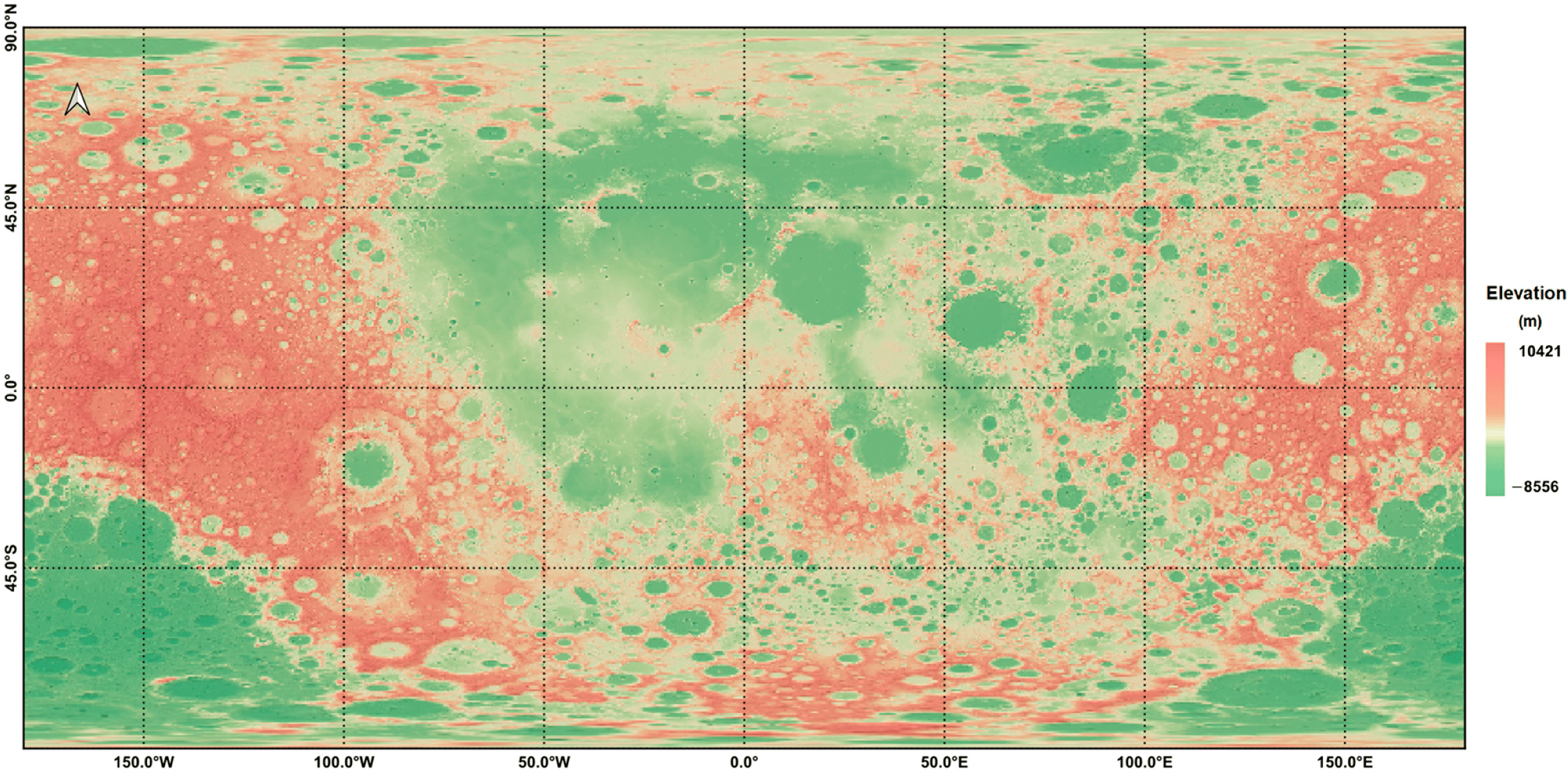
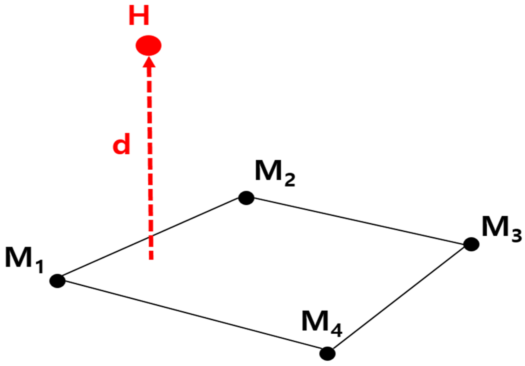
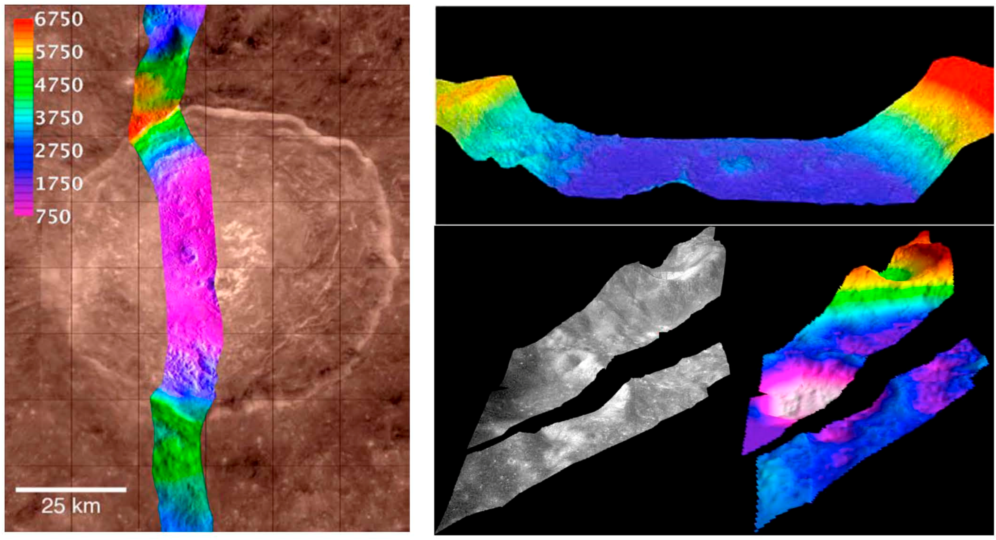
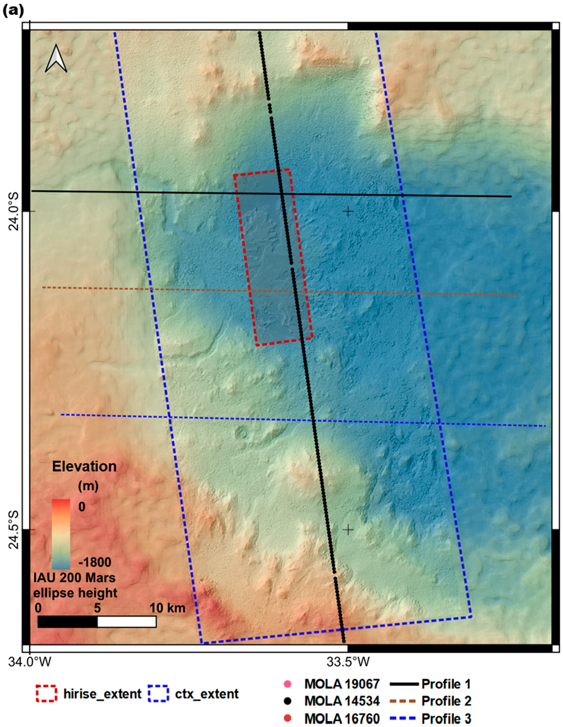
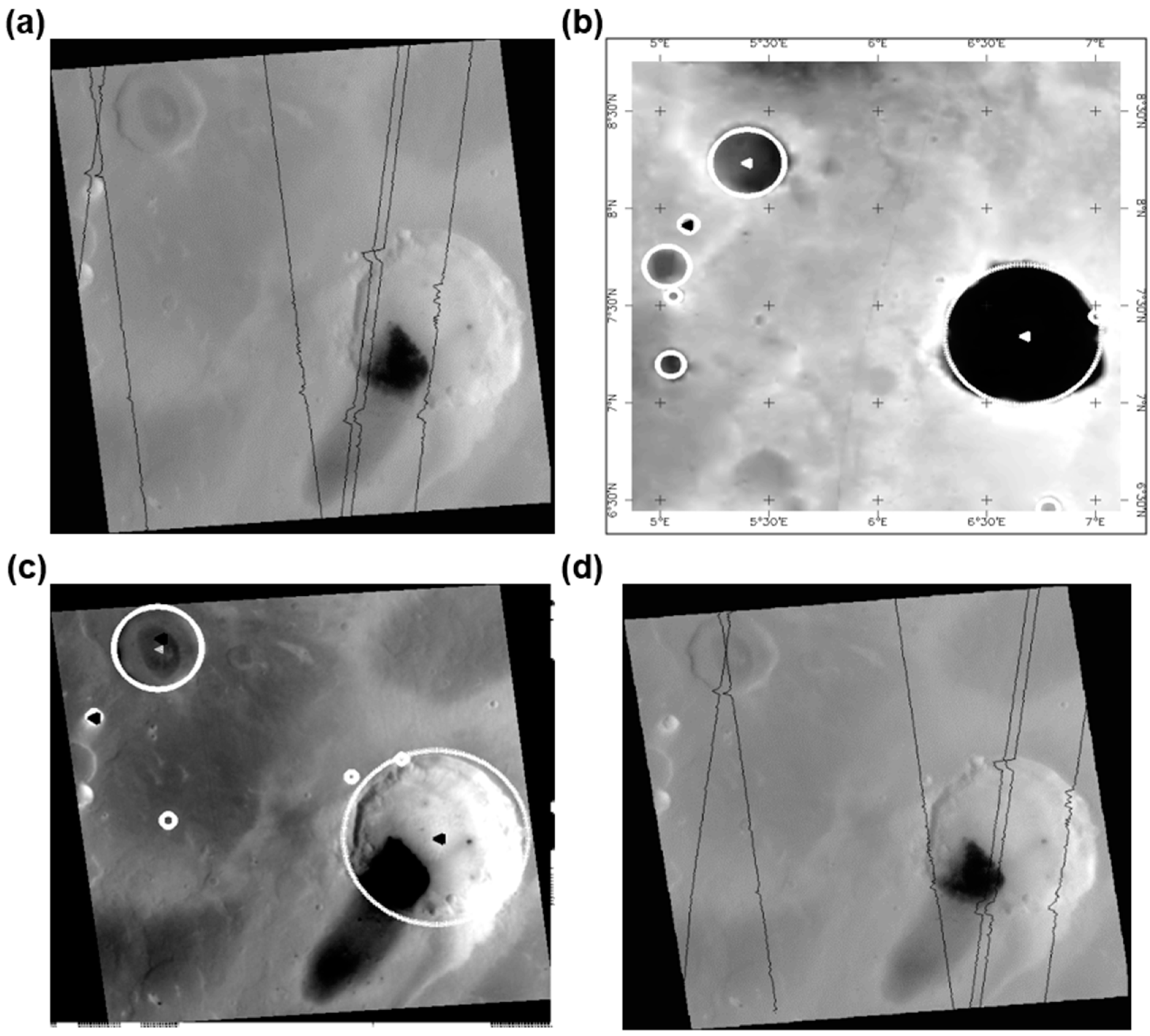
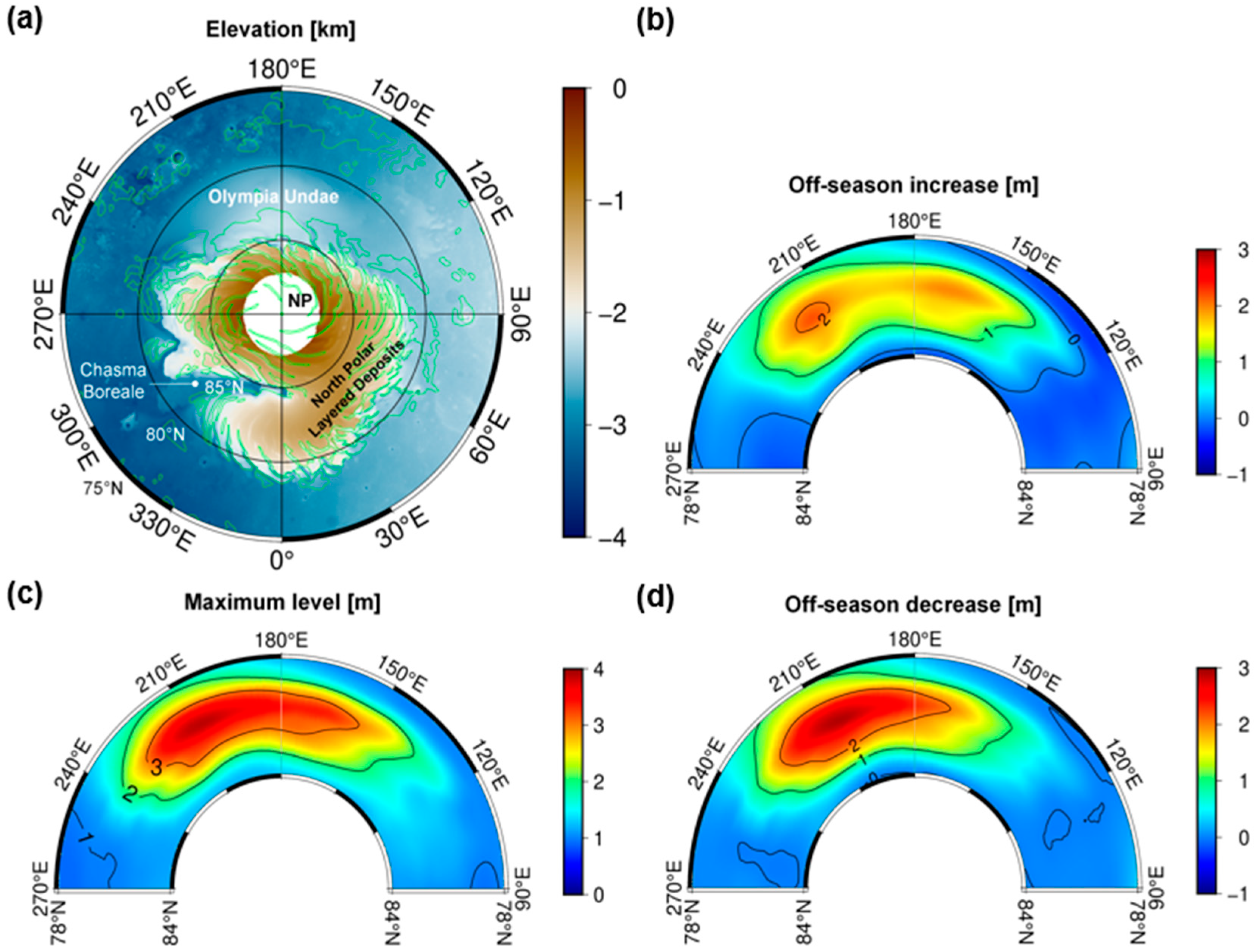
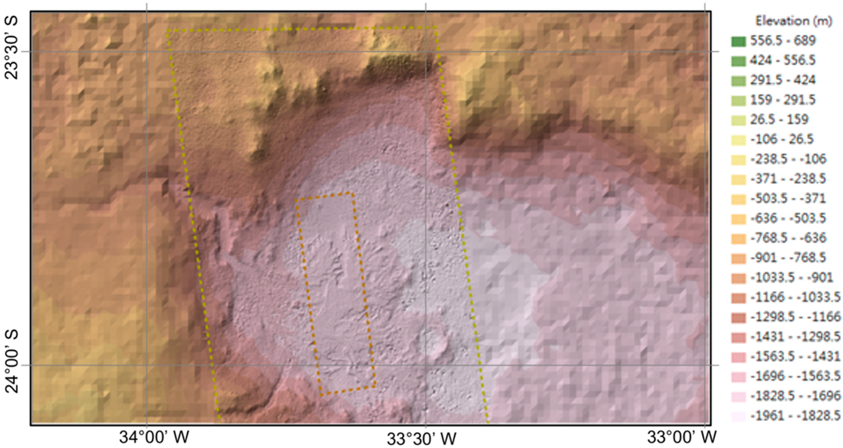
Figure 1. Topography of the Moon from LRO LOLA data. It is noted that this topographic map was produced based on the laser altimetry measurements and resampled with 118 m resolution. Details are in [42] (Data is available at https://astrogeology.usgs.gov/search/details/Moon/LRO/LOLA/Lunar_LRO_LOLA_Global_LDEM_118m_Mar2014/cub, accessed on 1 January 2023).
Remotesensing 15 02954 g001
Figure 2. The global topography of Mars from MOLA enhanced with stereo DEM (Data is available at https://astrogeology.usgs.gov/search/map/Mars/Topography/HRSC_MOLA_Blend/Mars_HRSC_MOLA_BlendDEM_Global_200mp, accessed on 1 January 2023).
Remotesensing 15 02954 g002
Figure 3. Structure of SPICE kernel taken/modified from [197].
Remotesensing 15 02954 g003
Figure 4. The relation between an HRSC intersection point and a bilinear surface defined by the MOLA DEM, where H is the HRSC intersection point, M1 to M4 are apex points of the MOLA DEM mesh and d is the distance between the HRSC and the MOLA DEM surface [207].
Remotesensing 15 02954 g004
Figure 6. Stereo DEMs over the Martian Jezero crater constructed the multi-resolution approach and non-rigorous sensor model [214] (a) 50 m resolution HRSC DEM by the DLR-VICAR system. (b) 12 m CTX DEM overlayed on the HRSC DEM. (c) 1 m HiRISE DEM overlayed on the CTX DEMs. Note the accuracy of registration, which is revealed in the comparison to the background DEMs.
Remotesensing 15 02954 g006
Figure 7. The schematics of centroiding the received pulse as a function of time (t) and signal strength (P), where P0 is the transmitted power, E0, Er is the transmitted/recevied energy, ΔT0 is a signal strength of one half of maximum [231].
Remotesensing 15 02954 g007
Figure 8. The effect of local slope on laser altimeter geolocation accuracy with footprint size (W), range error (ΔZ) by pointing angle and it’s error term (φ, Δφ) and the surface slope (S) [231,233].
Remotesensing 15 02954 g008
Figure 9. (a) Cassini SAR image coverages on the Titian surface through flyby T 77 demonstrating overlapping images forming the northern (blue) and southern (red) control networks (image taken from [178]). Refer to Lopes et al. [251] for more details. (b) Color-coded topographic map overlaid on a mosaic of SAR and high-altitude SAR images covering a southern polar region of Titan, derived from Cassini radar stereo analysis [178]. (c) Titan Cassini SAR mosaic and topography and constructed from Spherical harmonic expansion (SHE) analysis [252], which was fitted from RADAR altimetry and SARTopo data [177,182] (Data is available at https://astrogeology.usgs.gov/maps/titan-Cassini-global-topographic-data-record, accessed on 1 January 2013). (d) The outcome of the analysis of the T16-T19 pair using the Cassini SAR stereo radar image [243].
Remotesensing 15 02954 g009
Figure 10. (a) Radar altimetric DEMs overlayed on Magellan SAR mosaic (https://astrogeology.usgs.gov/search/map/Venus/Magellan/RadarProperties/Venus_Magellan_Topography_Global_4641m_v02, accessed on 1 January 2013) [95]. (b) Stereo DEM (675 m) on Joliot-Curie (06S066) FMAP quadrangle. (c) Stereo DEM (3°S–0°, 73°E–73.5°E) (orthoimage, global gridded altimetry (GTDR) DEM, and other three stereo DEMs (the details described in [107]). (b,c) were taken from Kirk et al. [107]. Refer to Herrick et al. [249] for another stereo DEM in Tellus Regio, a Venusian highland.
Remotesensing 15 02954 g010
Figure 11. A case of MiniSAR stereo analysis for DEM and Orthorectified Clementine UVVIS base mosaic image creations on part of Jackson crater. Stereo-derived elevations aligned to the LOLA altimetry track [250]. Images were taken from [250].
Remotesensing 15 02954 g011
Figure 12. (a) The population of 37,652 control (or tie) points in the MDIM 2.1 network [260], which is available at https://astrogeology.usgs.gov/search/map/Mars/Viking/MDIM21/Mars_Viking_MDIM21_Mosaic_global_232m (accessed on 28 March 2023). (b) Io control networks on the Galileo SSI and Voyager image mosaics (available at https://astrogeology.usgs.gov/search/details/Io/ControlNetworks/Io_data, accessed on 28 March 2023) [261] (c) Europa control network (https://astrogeology.usgs.gov/search/details/Europa/ControlNetworks/Europa_data, accessed on 28 March 2023) [261]. (d) Enceladus control network (https://astrogeology.usgs.gov/search/details/Enceladus/ControlNetworks/Enceladus_data, accessed on 28 March 2023) [262]. Note the radius values of the Europa 3D control network converge to a single value due to the accuracy of the bundle block adjustment model on the extremely flat terrain of Europa.
Remotesensing 15 02954 g012
Figure 13. (a) Co-registered DEMs over Eberswalde Crater, Mars. (b) Track profiles crossing HRSC-CTX-HiRISE DEMs created by multiple resolution approach [214]. RMSE of MOLA-HRSC, MOLA-CTX, and MOLA-HiRISE DEMs are 39.415, 44.052, and 17.404 m respectively.
Remotesensing 15 02954 g013aRemotesensing 15 02954 g013b
Figure 14. The registered MOC image (M0302925) over craters on MOC images. (a) The original offset between MOLA and MOC. (b) Crater detection on MOLA. (c) Crater detection on a MOC WA image, (d) Registration of the MOLA track on a MOC image using the detected craters.
Remotesensing 15 02954 g014
Figure 15. The LISFLOOD–FP hydrodynamic simulation on the HRSC image mosaic after bundle block adjustment (Athabasca Valles, Mars) (a) Assigned the location of Athabasca Valles and the domain of simulation (blue box). (b) Final LISFLOOD–FP hydrodynamic simulation in the d + 150 time domain.
Remotesensing 15 02954 g015
Figure 16. (a) Topography of the Martian north pole represented by the reference DEM from reprocessed and then self-registered MOLA altimetric profiles [421]. The missing coverage poleward of 87°N is due to a lack of nadir-pointed profiles as a result of the orbital inclination of the spacecraft. The map projection is North Polar Stereographic, with coverage poleward of 75°N and a spatial resolution of 1 km/pixel. The Olympia Undae dune fields, Residual North Polar Cap (green polygons), Chasma Boreale, and the layered deposits mainly made up of water ice and dust are marked. Spiral troughs are carved by katabatic winds associated with Mars’ rotation and Coriolis forces in (c) The maximum thickness of the seasonal deposits within Olympia Undae, which mainly covers 78°N to 84°N and 90°E to 270°E. Magnitudes of off-season decreases in thickness the northern winter (refer (b)) and off-season increases in the northern spring presented in (d) within Olympia Undae.
Remotesensing 15 02954 g016
Figure 17. TIN representation of multi-resolution DEMs of Eberswalde Crater. The base is the HRSC DEM. The CTX and HiRISE DEMs were outlined with yellow and orange boundaries, respectively. From the color of TIN along the boundaries, it is clear to observe that the co-registered DEM maintains consistency with the degree of variation in surface heights derived from HRSC.
Remotesensing 15 02954 g017
Table 1. Specifications of topographic mapping equipment installed on SELENE, Chang’e 1, Chandrayaan-1, and Lunar Reconnaissance Orbiter (LRO).
MissionLaunch YearSensorConfigurationResolution
SELENE2007Terrain camera (TC) [36]Two cameras (stereo)10 m (Spatial)
Laser altimeter (LALT) [37]Nd:YAG laser shot with pulse interval of 1 Hz5 m (Elevation)
Chang’e 12007Terrain camera (TC) [19]Three-line array CCD stereo camera120 m (Spatial)
Laser altimeter (LAM) [38]Nd:YAG laser shot with 1 s interval60 m (Elevation)
Chandrayaan-12008Terrain mapping camera (TMC) [39]Three cameras (stereo)10 m (Spatial)
Lunar laser ranging instrument (LLRI) [40]Pulsed Nd:YAG laser with 10 measurements per second10 m (Elevation)
LRO2009Lunar Reconnaissance Orbiter camera (LROC) [41]Two narrow angle cameras (NACs)0.5 m (Spatial)
One wide angle camera (WAC)100 m (Spatial)
Lunar orbiter laser altimeter (LOLA) [42]Nd:YAG laser transmitter with 28 Hz1 m (Elevation)
Table 2. MOLA Instrument Specifications (https://attic.gsfc.nasa.gov/mola/, accessed on 28 March 2023).
Laser TypeQ-Switched, Diode-Pumped Nd:YAG
Wavelength1.064 micrometre
Laser energy40–30 mJ pulse−1
Laser power consumption13.7 W
Pulse width~8.5 ns
Pulse repetition rate10 s−1
Beam cross-section25 × 25 mm2
Beam divergence0.25 mrad
±Footprint size (at 400 km)120 m
Footprint spacing (a velocity = 3 km/s) (center-to-center, along-track)300 m
Table 3. SPICE Kernel description [198].
SPICE Kernel NameInformation
CKPointing data for an instrument
EKSpacecraft and science instrument events including science plan (ESP), sequence of events (ESQ) and experimenter’s notebook (ENB)
IKInstrument mounting, field of view,
axis specification
LSKTransformation value between Universal
Time coordinates and Ephemeris
PcKAltitude and body shape information (size, shape and orientation)
FKReference frame specifications
SLCKSpacecraft clock coefficients
SPKSpacecraft, orbiter and planet/satellite body trajectory
Table 4. The accuracy of object point coordinates of the ray intersection [210].
Orbit NumberAltitude (km)σX (m)
(without/with Bundle Adjustment)
σY (m)
(without/with Bundle Adjustment)
σZ (m)
(without/with Bundle Adjustment)
18275–34712.1/6.610.7/6.033.4/18.1
22311–94113.0/8.617.2/9.141.6/21.9
68269–50531.2/11.029.2/10.450.6/17.9
Table 5. Euler angles for MOC WA, NA and MOLA [79].
InstrumentRoll (Degree)Pitch (Degree)Yaw (Degree)
MOLA−0.00290−0.008600.05900
MOC-NA0.11463−0.071620.18000
MOC-WA R1.04764−0.45229−0.78644
MOC-WA B1.01022−0.35472−0.30189
Disclaimer/Publisher’s Note: The statements, opinions and data contained in all publications are solely those of the individual author(s) and contributor(s) and not of MDPI and/or the editor(s). MDPI and/or the editor(s) disclaim responsibility for any injury to people or property resulting from any ideas, methods, instructions or products referred to in the content.

