Article

A Model-Assisted Combined Machine Learning Method for Ionospheric TEC Prediction

1
School of Microelectronics, Tianjin University, Tianjin 300072, China
2
Qingdao Key Laboratory of Marine Information Perception and Transmission, Qingdao Institute for Ocean Technology, Tianjin University, Qingdao 266200, China
3
Shandong Engineering Technology Research Center of Ocean Information Awareness and Transmission, Qingdao 266200, China
*
Author to whom correspondence should be addressed.
Remote Sens. 2023, 15(12), 2953; https://doi.org/10.3390/rs15122953
Submission received: 27 April 2023 / Revised: 29 May 2023 / Accepted: 31 May 2023 / Published: 6 June 2023

Abstract

:
In order to improve the prediction accuracy of ionospheric total electron content (TEC), a combined intelligent prediction model (MMAdapGA-BP-NN) based on a multi-mutation, multi-cross adaptive genetic algorithm (MMAdapGA) and a back propagation neural network (BP-NN) was proposed. The model combines the international reference ionosphere (IRI), statistical machine learning (SML), BP-NN, and MMAdapGA. Compared with the IRI, SML-based, and other neural network models, MMAdapGA-BP-NN has higher accuracy and a more stable prediction effect. Taking the Athens station in Greece as an example, the root mean square errors (RMSEs) of MMAdapGA-BP-NN in 2015 and 2020 are 2.84TECU and 0.85TECU, respectively, 52.27% and 72.13% lower than the IRI model. Compared with the single neural network model, the MMAdapGA-BP-NN model reduced RMSE by 28.82% and 24.11% in 2015 and 2020, respectively. Furthermore, compared with the neural network optimized by a single mutation genetic algorithm, MMAdapGA-BP-NN has fewer iterations ranging from 10 to 30. The results show that the prediction effect and stability of the proposed model have obvious advantages. As a result, the model could be extended to an alternative prediction scheme for more ionospheric parameters.

Graphical Abstract

1. Introduction

The ionosphere is an important part of the near-ground space environment. It is 60–1000 km above the ground and is an area where the excitation of high-energy solar radiation and cosmic rays ionizes the earth. The ionosphere consists mainly of charged particles, neutral atoms, and molecules. In the Sun–Earth space environment, the ionosphere is one of the most important parts directly affecting human space activities [1]. The ionosphere is a medium for radio wave transmission and a link between magnetic layers and a neutral atmosphere. The formation of ionizing layers and its changes are comprehensively controlled by various factors such as solar electromagnetic radiation, particle radiation, magnetic field disturbance, geomagnetic field change, and upper atmospheric movement, showing complex weather-like and climate-like variations, which will have a serious impact on satellite navigation, radar imaging, short-wave communication, and other technical means involving radio propagation and electromagnetic environment. The important characteristics parameters of the ionospheric characteristics include the critical frequency, profile height, total electron content (TEC), etc. These parameters are also widely used in satellite communication, navigation timing, radar detection, direction finding and positioning, spectrum management, and other civil and military fields [2]. Among them, TEC refers to the total number of electrons along the signal propagation path. It is an important parameter for analyzing the temporal–spatial distribution, morphological structure, delay characteristics, and disturbance of the ionosphere [3]. Using satellite observation data to solve TEC will cause TEC data to lag relatively. TEC can be estimated in near-real-time using a certain ionospheric model [4]. Accurately predicting TEC is not only very important to ensure the stability of the radio system but also very significant in pre-earthquake identification and other fields. These predictions are also essential for many aerospace and astronomical observation applications.
Due to the complexity of the ionosphere, many methods have been used for TEC modeling [5,6,7]. One of the models is the TEC prediction model established based on statistical experience. The most representative model is the International Reference Ionosphere (IRI) model. It is a well-known empirical model and is a recommended international standard [8,9,10]. The other is the empirical model of parameter prediction established by the ionosphere parameter observation data. This type of model is widely used in the forecast of ionosphere parameters due to its simple model structure and easy calculation.
In order to improve the prediction accuracy of ionospheric parameters, the artificial intelligence method was introduced [11] to predict the critical frequency of the F2 layer (foF2) [12], the 3000 km transmission factor of the F2 layer (M(3000) F2) [13], TEC [14], peak height [15], and other parameters [16]. In particular, the rapid development of machine learning [17] and intelligent computing technology provides more abundant prediction methods for nonlinear and nonstationary ionospheric parameter data. For example, the regional long-term prediction method based on statistical machine learning using the principal component method [14] and the long-term prediction method using the autocorrelation prediction method [18] are both intelligent prediction algorithms. In addition, through the extrapolation method based on physical observation without the input of prediction interval, a new TEC prediction method for the Arctic region is proposed using data from the past 14 years [19].
A deep learning algorithm, such as a neural network (NN), is a very important ionospheric parameter prediction method and has been widely used in recent years [17,20,21,22]. It often requires a large amount of data for training, so it has a good effect when dealing with large samples of data for a long time. It is very important to improve the prediction accuracy of ionospheric parameters, which is also a very popular research content [6,7]. The improvement and optimization of deep learning algorithms are significant means to improve the prediction accuracy of ionospheric parameters. The genetic algorithm (GA) can optimize the neural network to establish a short- or long-term prediction model of ionospheric parameters in a single station or a certain region and can get good results [23,24,25]. There are also some innovative optimization algorithms used to improve neural networks. For example, the artificial neural network (ANN) based on multi-source data and optimized by the genetic algorithm can be used to build a global ionospheric model for predicting various ionospheric parameters such as foF2 and hmF2 [26]. The radial basis function (RBF) neural network classification algorithm based on partial least squares (PLS) and GA (PLS-GA-RBF) is proposed to solve some recognition problems caused by small samples. The results indicate a good picture of the PLS-GA-RBF algorithm; the operating efficiency and recognition accuracy improved substantially [27]. The prediction accuracy of ionospheric parameters based on the backpropagation neural network (BP-NN) can be improved by using an improved particle swarm optimization algorithm [28].
In order to improve the long-term prediction accuracy of TEC, a new combined intelligent prediction algorithm was proposed by combining the IRI model, TEC statistical learning model, artificial neural network, and genetic algorithm. Furthermore, to improve the prediction accuracy, the weight and threshold of BP-NN are optimized by an adaptive genetic algorithm with a multi-mutation and multi-cross location.
The detailed arrangement of this paper is as follows: Section 2 is the modeling data and processing process; Section 3 proposes the model principle and modeling process; in Section 4, the predicted results are compared with the measured data and the predicted data of other models to verify the practicability of the method.

2. Materials and Methods

2.1. Materials

2.1.1. Data Collection

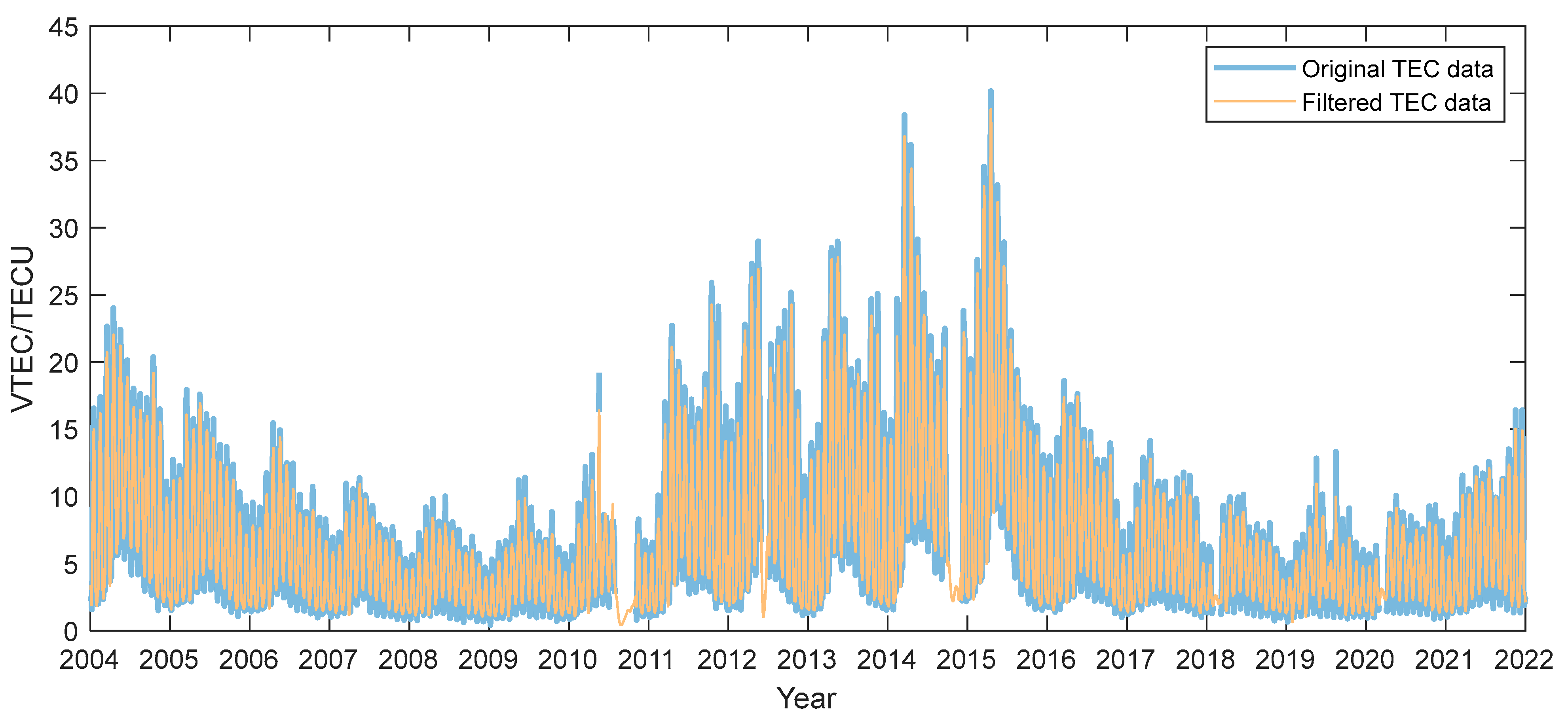
The modeling data used in this paper are divided into three parts: the TEC observation data of Athens Station, the solar radio wave flux of 10.7 cm wavelength (F10.7), and the sunspot number (SSN). In this paper, we can download the required TEC observation data by selecting the corresponding time, observed station, and data type through the official websites of the National Oceanic and Atmospheric Administration (NOAA) [29] and the Global Ionospheric Radio Observatory (GIRO) [30,31]. The downloaded data can be saved as a text file that records 24 h of TEC data for each day of the year at a station. In order to meet the modeling requirements of the Long-term regional ionospheric TEC prediction model, the monthly 24-h TEC mean values of each TEC observation station are calculated, and one observation station corresponds to a standardized modeling data file. As shown in Figure 1, by observing data, it can be found that TEC presents a certain periodic fluctuation, and the intensity of different years of fluctuations varies in different years. After the statistics of the above data, 5184 sets of data were obtained.

2.1.2. Data Processing

Here, we first preprocessed the TEC data by filtering. In this paper, mean filtering is used to filter the data. In order to ensure that the filtered data waveform is close to the original data waveform and to achieve the effect of suppressing interference and supplementing missing data points, we may use the data in an appropriate time window to carry out mean filtering. For each TEC data, the three values before and after the TEC data and itself were taken, and their mean value was calculated as the filtered data.
TEC i f = k = 1 3 TEC i k + TEC i + k = 1 3 TEC i + k ,
where  TEC i f  is the filtered TEC, and the  TEC i  is the original TEC. The processing in the following text is based on filtered TEC.
After the mean filtering of the original data, the missing data in the data set was supplemented with the fitting data of cubic spline interpolation, and the scatter plot was drawn and connected to compare with the original data, as shown in Figure 2. It can be found that, compared with before denoising, the fluctuation amplitude of the data after denoising is reduced, supplementing the missing data points in the dataset.
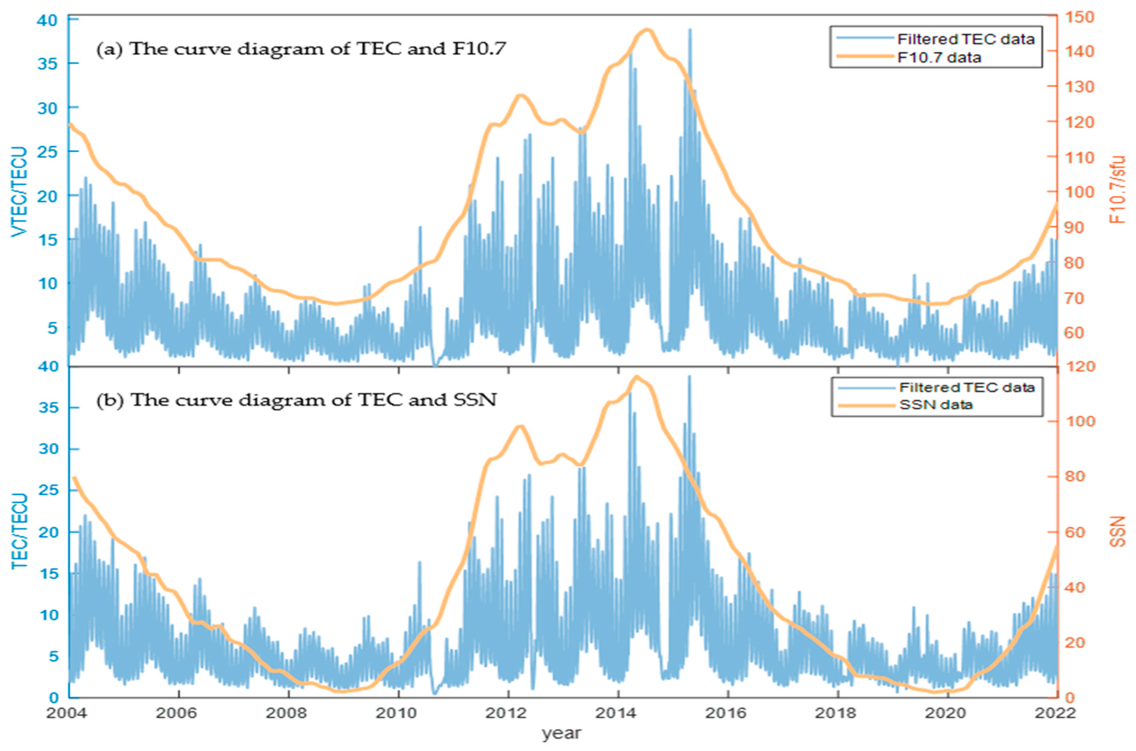
For F10.7, a scatter plot is drawn in time order and connected. TEC data and F10.7 were drawn on the same image, as shown in Figure 3a. Similarly, the same processing was performed on SSN, as shown in Figure 3b. It can be found that the overall variation of TEC data is strongly similar to the F10.7 data and SSN.

2.2. Methods

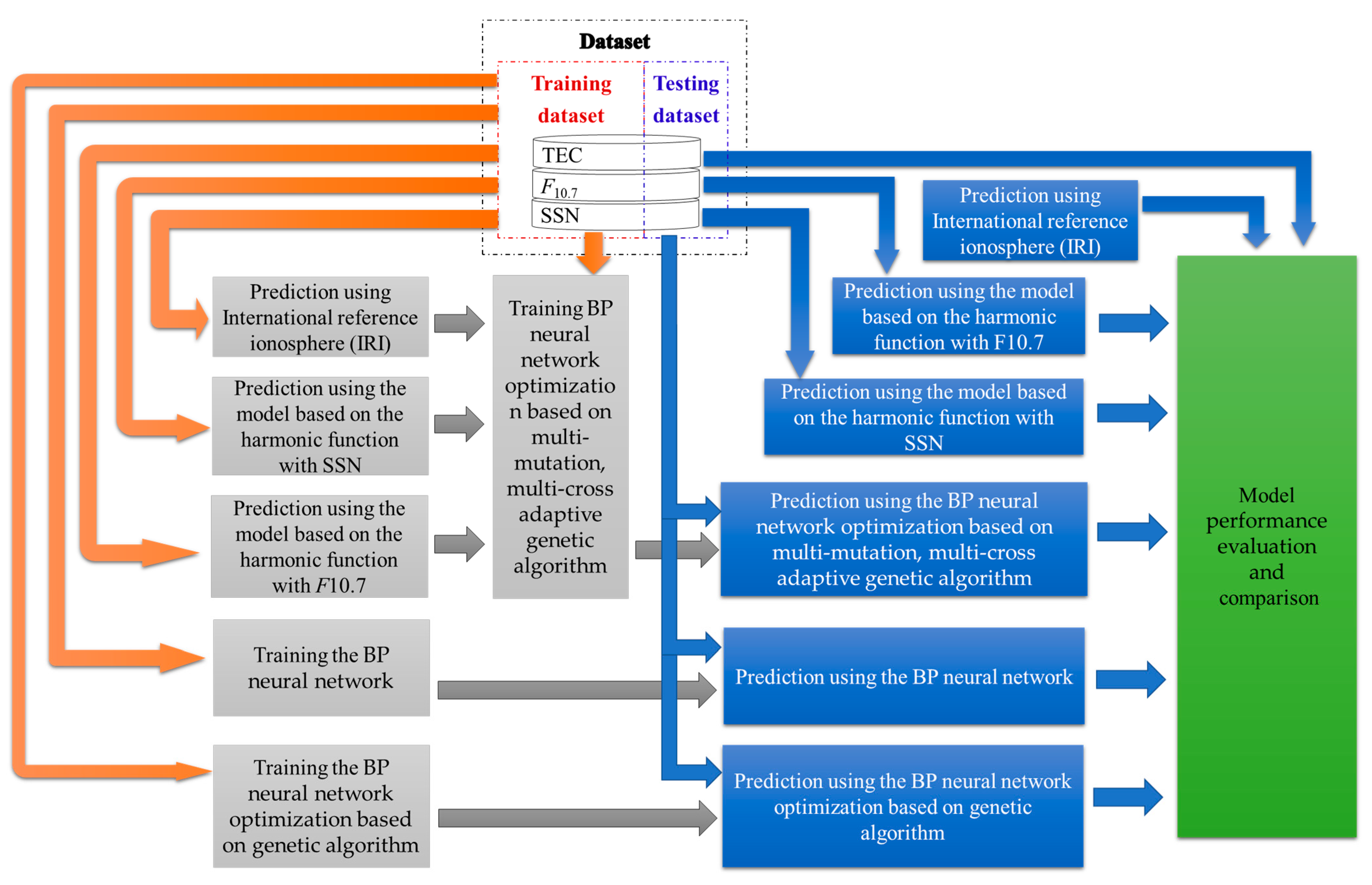
As shown in Figure 4, this paper combines several classical models and statistical machine learning (SML) models to obtain a high-accuracy prediction model. The prediction and validation of the combined model constructed in this paper mainly include four processes:
Step 1: Based on the statistical learning method, F10.7 and SSN were used to predict TEC.
Step 2: The IRI model was used to obtain TEC data in the prediction region.
Step 3: The BP-NN model is to predict final prediction results by training the data from the above IRI and statistical learning models, wherein the determination of the model using multi-mutation and multi-crossover adaptive genetic algorithm optimization algorithm.
Step 4: Compare the deviation between the TEC data predicted by the proposed model and the TEC data calculated by other models and the actual observed data, and analyze the capability gap between the proposed model and the existing model.

2.2.1. TEC Prediction Based on the IRI Model

The IRI model, a joint project of the International Union of Radio Science (URSI) and the Committee on Space Research (COSPAR) is the international standard for climate specifications of ionospheric parameters and an empirical model based on extensive terrestrial and spatial data [8,9]. It can describe the monthly mean value of electron density, electron temperature, ion temperature, and ion composition for a given location, data, and time in the non-auroral ionosphere over an altitude range of 50–1500 km. Since its inception in 1969, the IRI model has evolved with newer data and better mathematical descriptions of global and temporal patterns of change. In addition, numerous independent studies have validated the usability of the IRI model and compared it with direct and indirect ionospheric measurements not used in model development [9,32,33]. Therefore, the model used in this paper is IRI-2020 [34], through which the monthly one-hour average TEC data of Athens station from 2004 to 2021 are obtained for subsequent analysis and processing.

2.2.2. TEC Prediction Based on Statistical Machine Learning

Fourier expansion is known to be useful in characterizing periodic waveforms. Because TEC is inherently diurnal, Fourier analysis is superior to other ionospheric modeling methods in building empirical models of TEC predictions. In particular, the Fourier function was used to model the ionospheric TEC diurnal variation, with a period of 24 h, as shown in the following function [12]:
TEC λ , φ , m , p , s s n , T = n = 0 N a n λ , φ , m , p , s s n cos n T + b n λ , φ , m , p , s s n sin n T ,
where λ is the geographical latitude, φ is the geographical longitude, m is the month, p is the solar radio wave flux of 10.7 cm wavelength, ssn is the number of sunspots, T is the given time, expressed as between −180° and 180°, N is the maximum number of harmonics used to represent the diurnal variation and can be determined by the regression analysis, n (n = 1, 2, …, N) is the harmonic number,  a n    and  b n  are Fourier coefficients related to geographic coordinates and solar activity parameters.
For the given geographical location in Athens, Greece (38°02′N, 23°44′E, UTC/GMT + 2 h), the main factors affecting TEC are time and solar activity level. One of the determinants of solar activity level is F10.7, which is mainly determined by the corona and the upper layer of the chromosphere. Another determinant is SSN, which is influenced by the photosphere and the chromosphere. Therefore, we can predict TEC from solar cycle variation parameters and time parameters (year, semi-year, and month). The prediction function can be written as a harmonic function [12]:
TEC m , p = k = 0 K j = 0 J c k , j p p j cos 2 π km 12 + s k , j p p j sin 2 π km 12 ,
TEC m , s s n = k = 0 K j = 0 J c k , j s s n s s n j cos 2 π km 12 + s k , j s s n s s n j sin 2 π km 12 ,
where p is the average F10.7 over 12 months (unit is  10 22 / W / m 2 / Hz 1 ); ssn is the average SSN over 12 months; m is the month; K represents the upper limit of annual, semi-annual, seasonal, and monthly cycles; J represents the upper limit of solar cycles. K and J can be determined by regression analysis. In addition, the coefficients  c k , j p , s k , j p , c k , j ssn , s k , j ssn  in the formula were determined by the least square fitting method.
Either an empirical ionospheric model or a principle-based physical model is derived from observations. In exactly the same way, the ionospheric parameters of the above harmonic functions can be determined from observations. The root-mean-square error (RMSE) could be easily estimated with the least squares regression analysis for TEC [12,16]. The calculation shows that the maximum harmonic number N in Equation (2) is up to 11 in the above model to ensure the highest precision and robustness. Similarly, when the regression order J = 2 and K = 2 in Equations (3) and (4), the calculated RMSE of TEC is smaller. It can be seen that it has better convergence and stronger robustness.

2.2.3. Modeling of Neural Network Optimization Based on Genetic Algorithm

In this section, the TEC data predicted by solar activity level index, IRI-2020, and harmonic function fitting were taken as input, and TEC data were taken as output to establish a prediction model based on BP-NN. In addition, the multi-mutation and multi-crossover adaptive genetic algorithm (MMAdapGA) was used to optimize the model, and existing data (the actual filtered TEC data, time parameter (UTC), TEC data predicted by the IRI model, and the SML-based model, etc.) were used as training dataset and testing dataset to train the model.
ANN simulates the process of neuron signal transmission [35]. The neuron is a topological network established by biological research and the response mechanism of the brain, simulating the process of neural conflict. The end of multiple dendrites receives external signals and transmits them to neurons for processing and fusion. Finally, the nerve is transmitted to other neurons or effectors through axons. ANN approximates complex nonlinear functions as an algorithm model of basic nonlinear function combinations. This model has been successfully applied to TEC modeling and prediction [35]. ANN does not need to determine the mathematical equation of the mapping relationship between input and output in advance. Through its own training, ANN can obtain the result closest to the expected output value when the input value is given.
As a classical algorithm, BP-NN simulates the neuronal processing process [36], which is a multi-layer feedforward network trained by error backpropagation. Its basic idea is the gradient descent method which uses the gradient search technology to minimize the mean square error of the actual output value and the expected output value of the network [37].
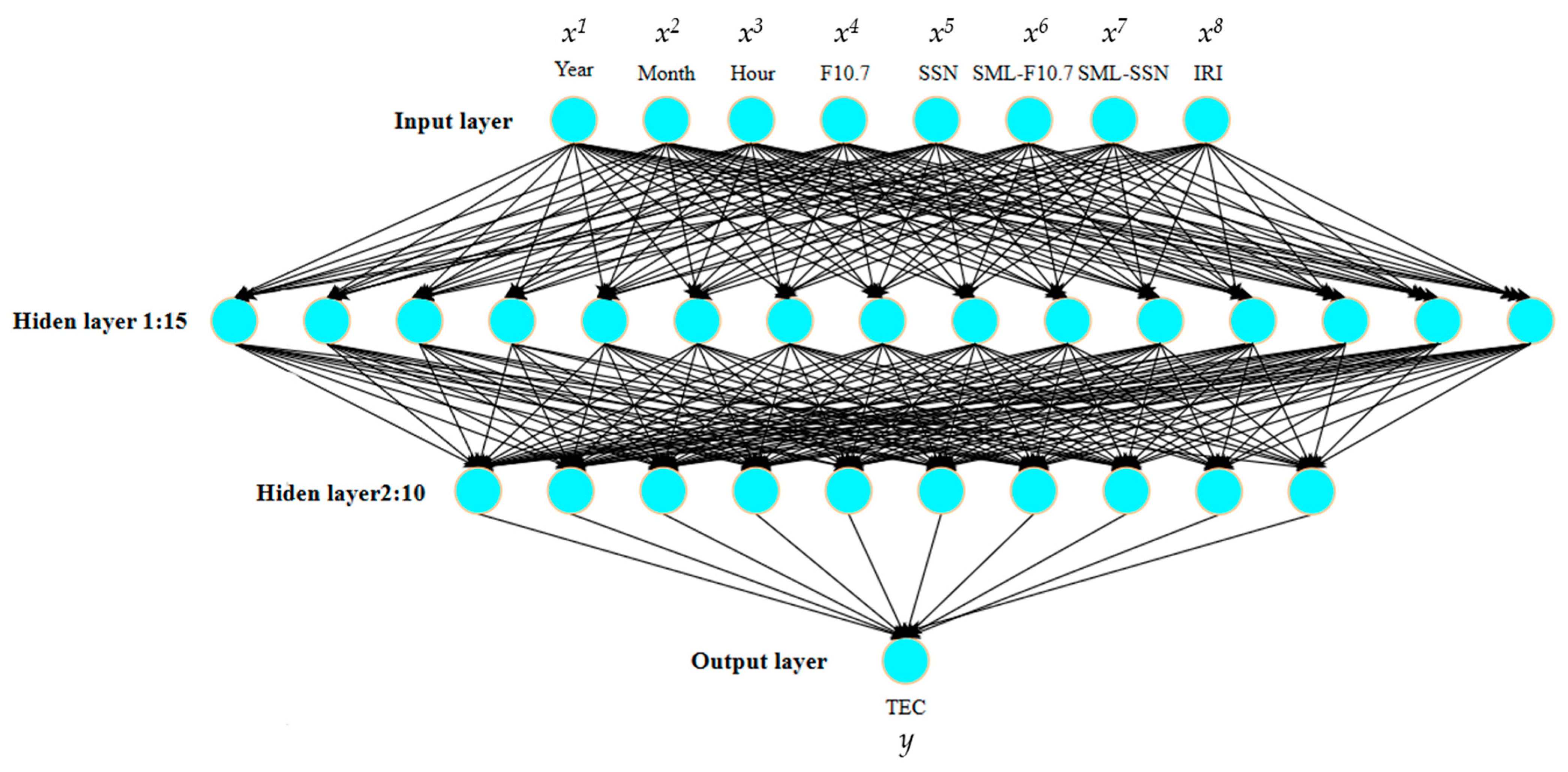
The input of BP-NN designed in this paper is respectively coordinated Universal Time UTC (year, month), F10.7 observation data, SSN observation data, SML-based model fitting TEC data through F10.7 (SML-F10.7), SML-based model fitting TEC data through SSN (SML-SSN), and the IRI model prediction TEC data. The output is the TEC prediction data. The input of the TEC data containing predictions of multiple models can solve the problem of a large deviation of a single model after a certain prediction time. The BP-NN constructed in this paper has a neural network with eight input neurons, one output neuron and two hidden layers. The first hidden layer comprises 15 hidden neurons, and the second hidden layer is composed of 10 hidden neurons, as shown in Figure 5.
The BP-NN model test dataset accounts for about 10% of the total dataset, and the training set accounts for about 90% of the total dataset. The training set is represented by the formula shown below:
D = x 1 1 , , x 1 8 , y 1 , x 2 1 , , x 2 8 , y 2 x n 1 , , x n 8 , y n .
The above neural network is trained. Each data set is normalized to [−1, 1] as a training set to carry out fitting training on the BP neural network model, in which the normalization formula is [38]:
y i = 2 x i x m i n x m a x x m i n 1 ,
for the neuron i (i = 1, 2, …, 15) in the first hidden layer,  x i 1 , x i 2 , , x i 8  is the input of the neuron. The input is the independent variable that has a key influence on the system model. The input in this model is eight kinds of data, as shown in Figure 5.
W i 1 1 , W i 1 2 , , W i 1 8  is the connection weight, which is used to adjust the weight ratio of each input. According to biology, neurons are activated only when the amount of information they receive reaches a threshold. Therefore,  Φ i 1  is used in this paper to represent the threshold value of this neuron, which is determined by the multi-mutation and multi-crossover adaptive genetic algorithm. Similarly, the connection weight of neuron r (r = 1, 2, …, 10) in the second hidden layer is  W r 2 1 , W r 2 2 , , W r 2 15 . The threshold value of this neuron is  Φ r 2 . The connection weight of the hidden layer to the output layer is  V 1 , V 2 , , V 10 . The threshold value is  Ψ . All activation functions in this paper are Sigmod functions [17].
S i g m o d x = 1 1 + e x ,
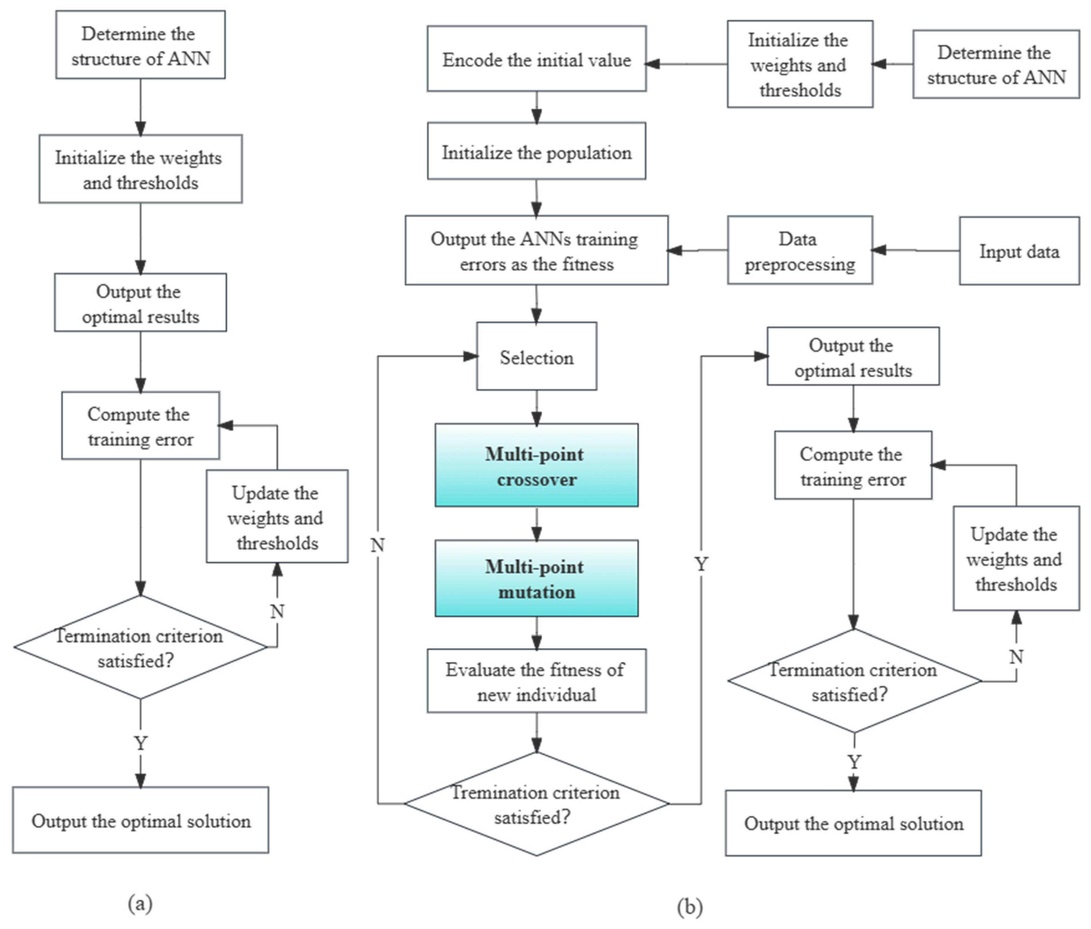
BP-NN is mainly composed of the topology structure of the neural network (number of input/output parameters, number of layers of neural network), the weight and threshold between each layer, and the training and prediction of the neural network. The algorithm flow chart of BP-NN is shown in Figure 6a. GA is a global optimization algorithm with good global search ability. The adaptive method mainly changes the individual crossover and mutation probability automatically with the change of fitness function value, which can improve the computational efficiency and accelerate the convergence rate of the algorithm [26]. Multi-mutation and multi-crossover can improve individual mutation rate and crossover rates and reduce the probability of local minimization resulting in a dead cycle [39]. The MMAdapGA can optimize the weight and threshold of BP-NN, improve the computational efficiency and accuracy of BP-NN, and reduce the error [25]. In this paper, MMAdapGA is used to calculate and optimize the weights and thresholds between each layer of BP-NN. The flowchart of the algorithm is shown in Figure 6b.
Since the topological structure of BP-NN has been determined, that is, the weights and thresholds between each layer of the neural network have been determined, then the number of optimization parameters of the genetic algorithm can be determined. In addition, the weights and thresholds of BP-NN are random numbers in the interval [−0.5, 0.5] initialized randomly, so the coding length of the individual population can be determined. In this paper, two crossover points and two mutation points are set, and the mating and mutation probabilities are changed automatically with the change of fitness function value. The optimization process of MMAdapGA for BP-NN is as follows:
Step 1: Population initialization. The individual coding method is real coding, and each individual is a real number string, which consists of six parts: the connection weight of the input layer and hidden layer, the connection weight of hidden layer and the hidden layer, a threshold of two hidden layers, connection weight of the hidden layer and the output layer, and threshold of the output layer. The individual contains all the weights and thresholds of BP-NN. Under the condition that the network structure remains unchanged, a neural network with definite structure, weights and thresholds can be formed.
Step 2: Fitness function. The initial weight of the neural network is obtained according to the individual. After training the neural network with training data, the TEC output is predicted. The sum of absolute error E between the predicted output  T E C f  and the expected output  T E C r  is used as the calculation formula for the individual fitness value.
E t = k j = 1 M TEC t j f TEC j r ,
TEC tj f  is the TEC value predicted by an input j in the data set, and the neural network population it uses is composed of a fixed topology structure and the threshold and weight obtained by decoding individual  a t TEC j r  is the expected output, namely the actual TEC value corresponding to j in the data set. k is the coefficient.
Step 3: Selection operation. Regeneration individuals are selected according to fitness. Individuals with high fitness have a higher probability of being selected, while individuals with low fitness are eliminated. It can be seen from Formula (8) that the fitness of individuals with smaller fitness values is higher, so the reciprocal of fitness values is taken to calculate the selection probability.
Step 4: Crossover operation. Since the individuals are coded by real numbers, the crossover operation method is the real number crossover method. Two random numbers need to be set to cross individuals, as two points are used for crossing operations. Let two crossing points cross at the same time. When crossing at the m time, the changes of individual  a k   ( k = 1 , 2 , , 135 )  and individual  a l   ( l = 1 , 2 , , 135 )  in the population can be expressed by the following formula:
a k m = a k m 1 b 1 + a l m b 1 a l m = a l m 1 b 2 + a k m b 2
where,  a k m  and  a l m  are individual  a k  and  a l  at the m crossover time.  b 1  and  b 2  are the random number in the interval of [0, 1].
Since the adaptive genetic algorithm is adopted, the probability of the cross operation of individual  a k  and individual  a l  is [40]:
P k l = k 1 E m a x E k l E m a x E a v g , E k l E a v g k 2 , E k l < E a v g ,
E m a x  is the maximum population fitness.  E a v g  is the average population fitness.  E k l = m a x { E k ,   E l }  is the larger adaptation value of individual  a k  and individual  a l k 1 = 0 . 3 ,   k 2 = 0 . 5  are the coefficients.
Step 5: Variation operation. Mutative operation is performed on a weight W or threshold V. Select gene  a k p  and gene  a k q  of individual  a k  for the mutation operation as follows:
a k p , q = a k p , q + a k p , q a m a x 1 g G max 2 r ,   r > 0.5 a k p , q + a m i n a k p , q 1 g G max 2 r , r 0.5 ,
where, r is a random number in the range of [0, 1]. g is the current iteration number.  G m a x  is the maximum number of evolutions.
Due to the adaptive genetic algorithm, the mutation probability of gene  a k p  in individual  a k  is expressed by the following formula:
P k p = k 3 E m a x E k E m a x E a v g , E k E a v g k 4 , E k < E a v g ,
where  E k  is the fitness of the individual  a k k 3 = 0 . 1 ,   k 4 = 0 . 2  are the coefficients.
Step 6: A new generation of population is generated from crossover and mutation, then return to Step 2. Repeat the process 100 times. Finally, the relative optimal solution of weights and thresholds of each BP-NN layer is obtained.
Step 7: The BP-NN is trained and optimized by MMAdapGA, and the error is calculated. The gradient descent method is used to update the weights and thresholds again. Finally, MMAdapGA-BP-NN with errors within the allowed range is obtained, and the model is tested by predicting the TEC of the test set.

3. Results and Discussion

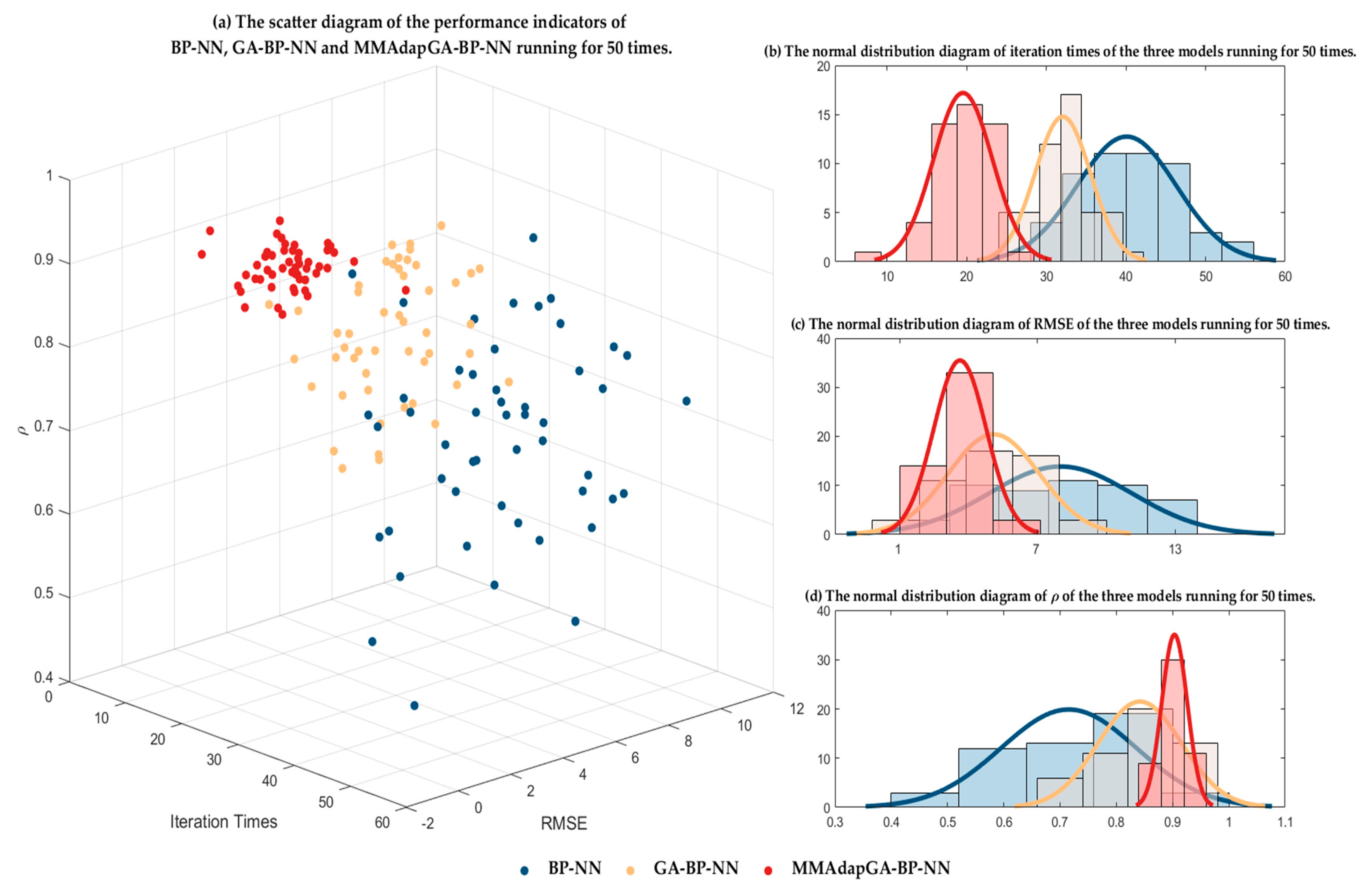
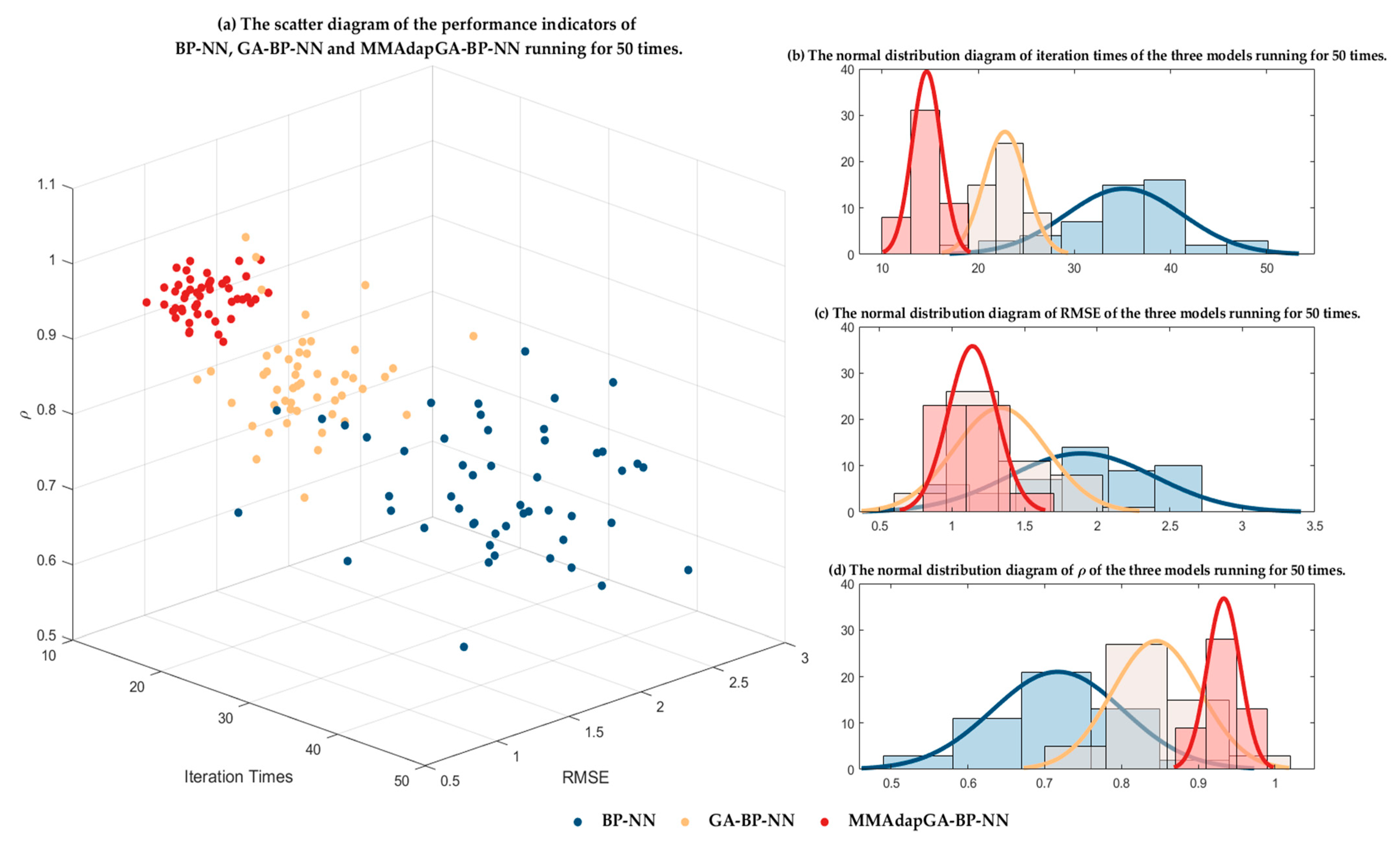
In this paper, the MMAdapGA-BP-NN prediction model is proposed. At the same time, a single BP-NN prediction model (prediction of TEC based on BP neural network) and GA-BP-NN prediction model (prediction of TEC based on neural network optimized by a single mutation and single crossover genetic algorithm) are proposed. As can be seen from Figure 3, 2015 is a year of high solar activity, and 2020 is a year of low solar activity. Data from 2015 and 2020 are taken as test sets, respectively, and other data are taken as training sets to train the model. In this paper, the above three models are all run 50 times, and the running results are analyzed. The performance of the above three models, the IRI model and the SML-based model, is compared and analyzed. The error between each predicted TEC data and the actual observed TEC data  e r r i  is defined in the following formula:
e r r i = TEC i f TEC i r .
The performance indicators are as follows [41]:
  • Mean Absolute Error (MAE)
    MAE = 1 N i = 1 N TEC i f TEC i r ,
  • Mean Relative Error (MRE)
    MRE = 1 N i = 1 N TEC i f TEC i r TEC i r × 100 % ,
  • Root Mean Square Error (RMSE)
    RMSE = 1 N × i = 1 N ( TEC i f TEC i r ) 2 ,
  • Correlation Coefficient ( ρ )
    ρ = i = 1 N ( TEC i f TEC f ¯ ) ( TEC i r TEC r ¯ ) i = 1 N ( TEC i f TEC f ¯ ) 2 i = 1 N ( TEC i r TEC r ¯ ) 2 .
In Equations (13)–(17),  TEC i f  is the predicted TEC data, and  TEC i r  is the actual observed TEC data.  TEC f ¯  is the average value of predicted TEC data, and  TEC r ¯  is the average value of actual observed TEC data.
The comparison results are shown in Table 1, where SML-F10.7 is the SML-based model for prediction based on the actual observed data of F10.7, and SML-SSN is the SML-based model for prediction based on the actual observed data of SSN.
By observing the performance indicators of each model in Table 1, it can be found that:
  • According to the high solar activity year (2015), low solar activity year (2020) and the mean values of the two years of performance indicators, the IRI model has the largest prediction error; the SML-based model has a slightly better prediction effect than the IRI model; MMAdapGA-BP-NN has the smallest prediction error and the best effect among all models.
  • The prediction results of all models are generally slightly better in a low solar activity year (2020) than in a high solar activity year (2015). The MAE, MRE, RMSE, and ρ of MMAdapGA-BP-NN decreased by 86.21%, 53.91%, 70.07%, and 3.30% in a low solar activity year (2020) compared with high solar activity year (2015).
  • In the year of high solar activity (2015), the MAE, MRE, RMSE, and ρ of MMAdapGA-BP-NN decreased by 45.28%, 57.26%, 52.27%, and 21.33% compared with the IRI model. In the year of low solar activity (2020), the MAE, MRE, RMSE, and ρ of MMAdapGA-BP-NN decreased by 85.42%, 80.58%, 72.13%, and 20.51% compared with the IRI model. On the whole, the MAE, MRE, RMSE, and ρ of MMAdapGA-BP-NN decrease by 58.87%, 51.84%, 58.01%, and 21.05% compared with the IRI model. Based on the above data, it is concluded that MMAdapGA-BP-NN is reliable for a long period of time.
  • In the year of high solar activity (2015), the MAE, MRE, RMSE, and ρ of MMAdapGA-BP-NN decreased by 25.91%, 27.86%, 28.82%, and 10.98% compared with BP-NN. In the year of low solar activity (2020), the MAE, MRE, RMSE, and ρ of MMAdapGA-BP-NN decreased by 31.71%, 41.39%, 24.11%, and 14.63% compared with BP-NN. Overall, the MAE, MRE, RMSE, and ρ of MMAdapGA-BP-NN decreased by 26.58%, 29.07%, 36.60%, and 9.52% compared with BP-NN. Based on the above data, it can be seen that the optimization effect of MMAdapGA on BP-NN is very obvious. Moreover, the optimization effect of MMAdapGA on BP-NN in a high solar activity year (2015) is more obvious than that in a low solar activity year (2020).
We record the operation results of BP-NN, GA-BP-NN and MMAdapGA-BP-NN TEC prediction models, respectively. The results of each model are recorded 50 times, as shown in Figure 7 and Figure 8.
It can be observed from Figure 7 and Figure 8 that:
  • MMAdapGA-BP-NN results of 50 runs generally have smaller RMSE, larger ρ, and better prediction accuracy.
  • In the year of high solar activity (2015), the average number of iterations converging for 50 running times of MMAdapGA-BP-NN, GA-BP-NN, and BP-NN are 19.5, 32.7, and 40.3, respectively. In the year of low solar activity (2020), the average number of iterations converging for 50 running times of the three models are 15.0, 23.3, and 33.5, respectively. MMAdapGA-BP-NN has fewer iterations and faster training speed.
  • In the year of high solar activity (2015), the standard deviations of iterations converging for 50 running times of MMAdapGA-BP-NN, GA-BP-NN, and BP-NN are 3.71, 3.95, and 4.12. The standard deviations of RMSE of the three models are 1.46, 2.15, and 3.57. The standard deviations of ρ of the three models are 0.08, 0.14, and 0.34, respectively. In the year of low solar activity (2020), the standard deviations of iterations converging for 50 running times of the three models are 2.14, 2.34, and 5.02. The standard deviations of RMSE of the three models are 0.74, 1.03, and 1.46. The standard deviations of ρ of the three models are 0.06, 0.12, and 0.23, respectively. Compared with GA-BP-NN and BP-NN, MMAdapGA-BP-NN has a lower standard deviation of performance indexes, and the training effect is more stable. Moreover, the three models are generally more stable in the low solar activity year (2020) than in the high solar activity year (2015).
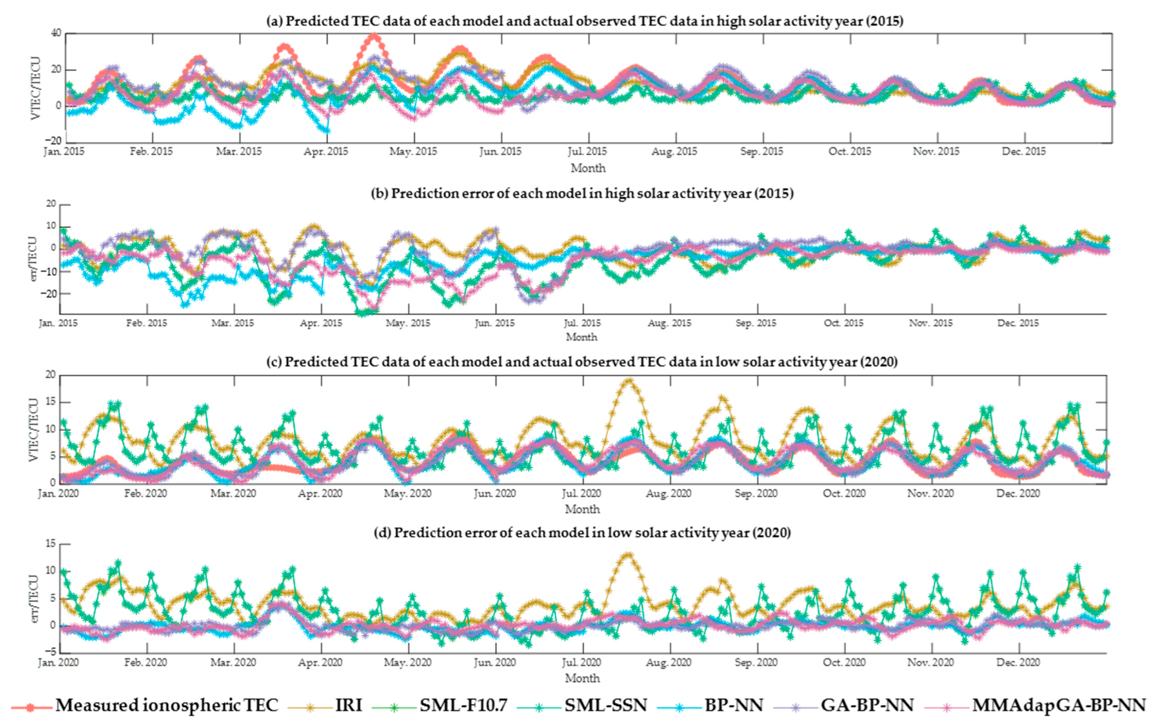
We calculated the mean value of the results of 50 runs of MMAdapGA-BP-NN, GA-BP-NN, and BP-NN, which are used as the average prediction results of the three models. The curve graph of actual observed TEC data and the scatter graph of predicted data of each model in a high solar activity year (2015) are shown in Figure 9a. The curve graph of the prediction error of the corresponding models is shown in Figure 9b. The curve graph of actual observed TEC data and the scatter graph of predicted data of each model in a low solar activity year (2020) are shown in Figure 9c. The curve graph of the prediction error of the corresponding models is shown in Figure 9d.
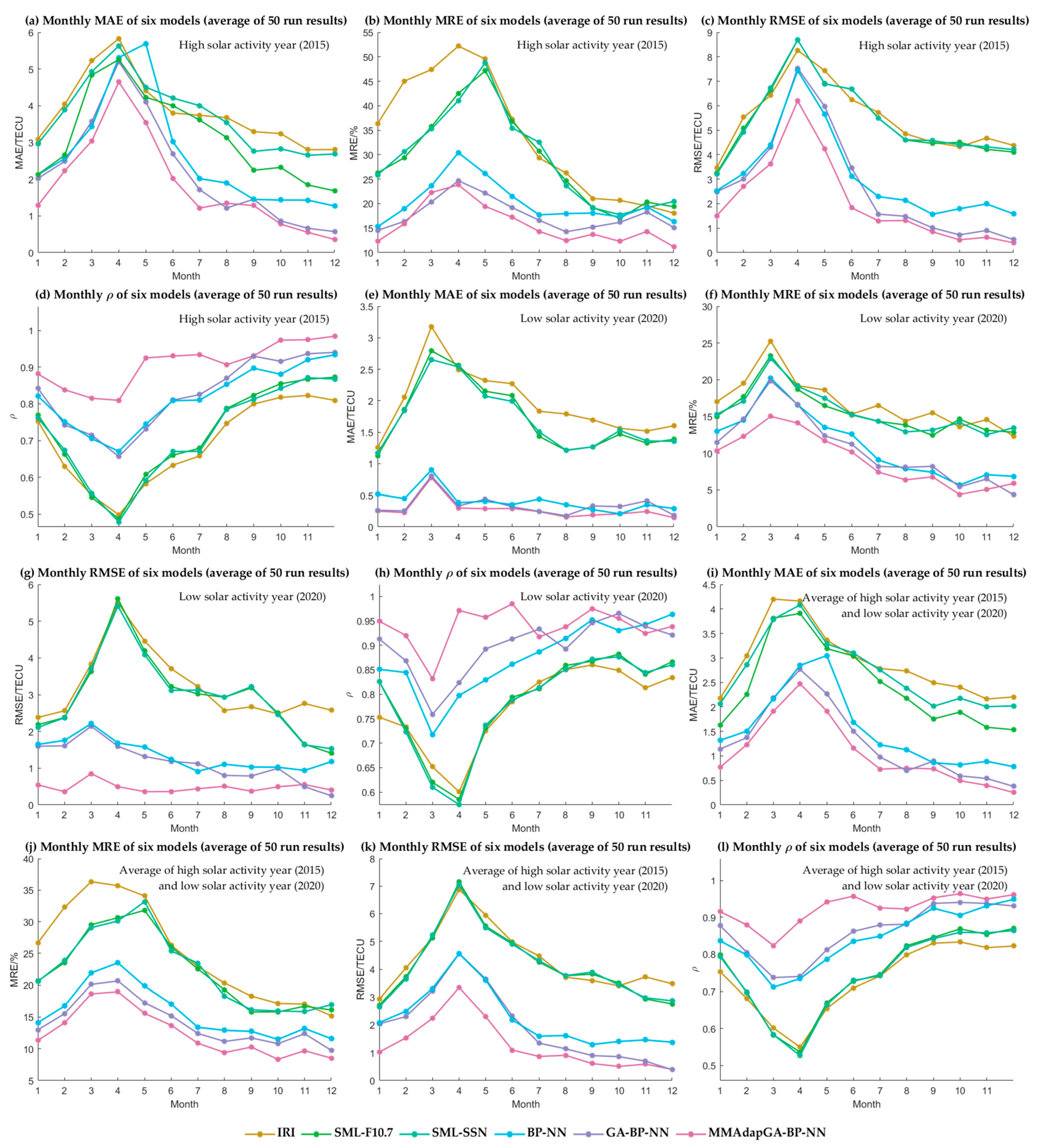
Monthly performance indicators (average of 50 runs) of the above six models in a high solar activity year (2015) and low solar activity year (2020) are calculated, and variation curves are drawn, as shown in Figure 10. In the months with high TEC fluctuations, the prediction effect of the model is poor. In March, April, and May 2015, actual observed TEC data were larger than the normal condition, and the forecast data of MMAdapGA-BP-NN showed large errors. In March and April 2020, actual observed TEC data were smaller than normal, and the MMAdapGA-BP-NN forecast data had larger errors than in other months. But in general, compared with other models, the prediction results of MMAdapGA-BP-NN are more accurate and stable.
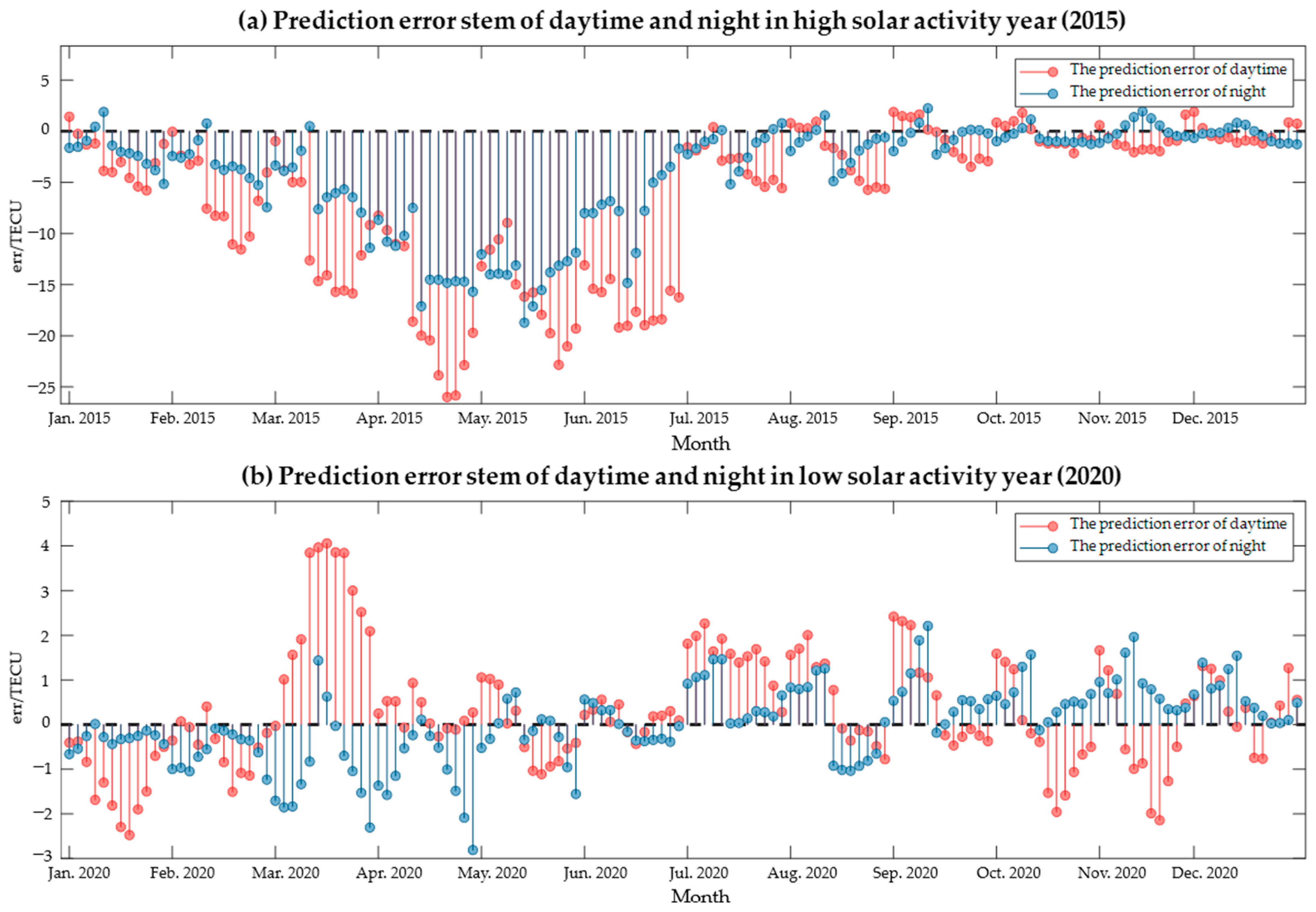
Taking 6:00 to 18:00 as daytime and the rest of the time as night, the diurnal deviation of the predicted results is analyzed. The deviation of TEC data in daytime and night predicted by MMAdapGA-BP-NN in the high solar activity year (2015) and low solar activity year (2020) is shown in Figure 11. The prediction error is large when actual observed TEC data fluctuate violently. Overall, the prediction error is smaller at night than during the daytime. The performance indexes of MMAdapGA-BP-NN in daytime and night in the high solar activity year (2015) and low solar activity year (2020) are calculated, as shown in Table 2. In the year of high solar activity (2015), MAE, MRE, RMSE, and ρ of MMAdapGA-BP-NN during the night decreased by 45.31%, 48.30%, 35.62%, and 14.63% compared with daytime. In the low solar activity year (2020), MAE, MRE, RMSE, and ρ of MMAdapGA-BP-NN during the night decreased by 48.65%, 60.70%, 39.42%, and 7.78% compared with daytime.
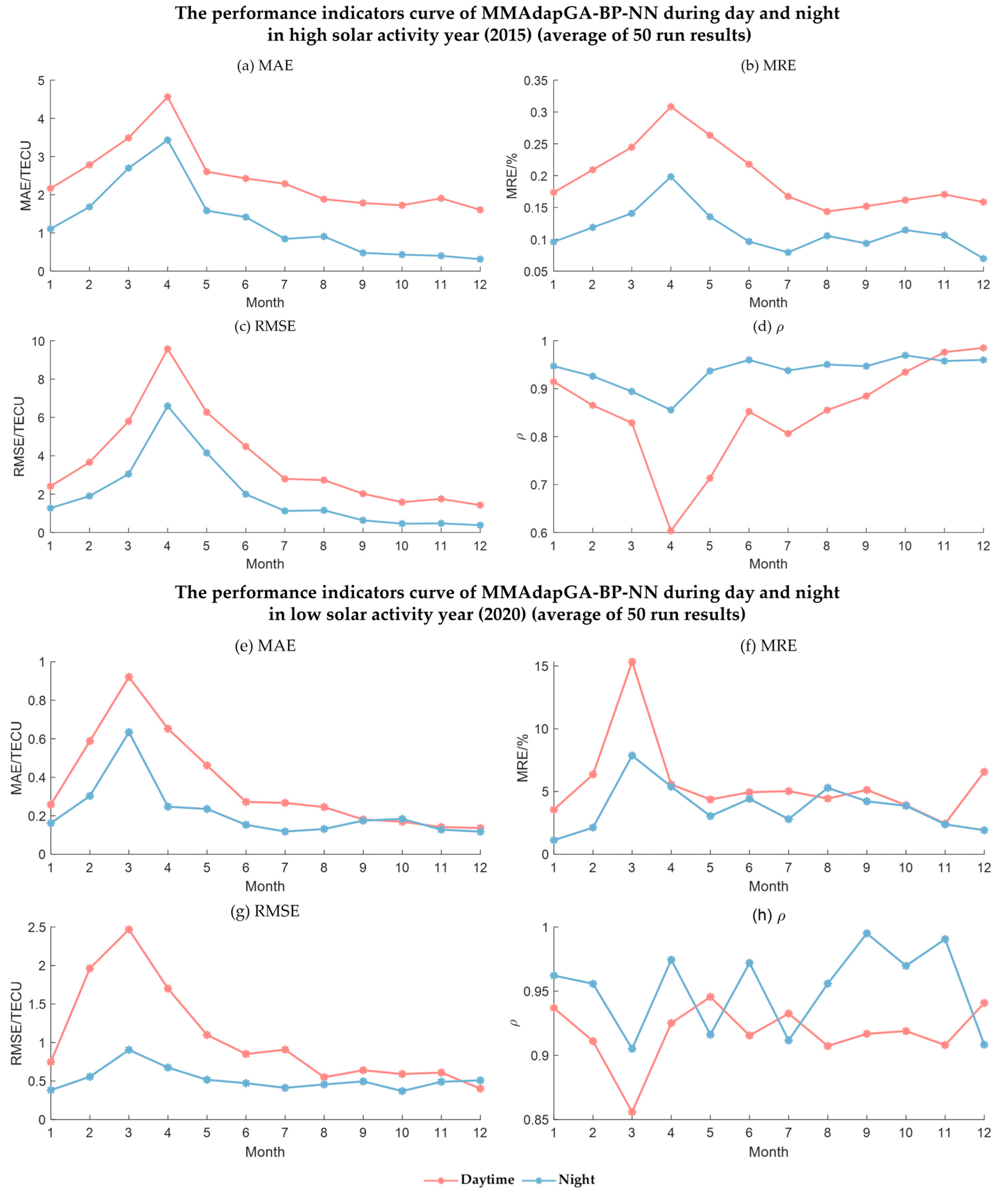
Monthly performance indicators of MMAdapGA-BP-NN in the high solar activity year (2015) and low solar activity year (2020) are calculated, respectively, and variation curves are drawn, as shown in Figure 12. Around April 2015 and March 2020, TEC data fluctuated sharply, and the prediction error was large. Obviously, the prediction error of TEC data during the daytime is generally larger than that at night.
Geomagnetic storms can cause the disturbance of TEC. Multiple storm periods occurred during the years 2015 and 2020 [42]. For example, a geomagnetic storm occurred on 17 March 2015 [43]. The impact of geomagnetic storm intensity on TEC prediction errors is analyzed next. And the Ap index can also characterize the geomagnetic storm intensity. The qualitative expression of geomagnetic storm intensity is shown in Table 3.
Furthermore, the qualitative analysis yields the number of  A p > 15  days and the number of  A p     30  days in high solar activity years (2015) and low solar activity years (2020), as shown in Figure 13. It can be found that there is no obvious correlation between the absolute error of predicted TECs and the geomagnetic storm days. In addition, the correlation coefficient ρ between the  A p  index, and the absolute error is calculated quantitatively and is −0.36 and 0.35, respectively. It can be found that the correlation coefficient between the  A p  index and the absolute error is small.

4. Conclusions

Real-time and accurate TEC monitoring is essential for many aerospace applications. The combined prediction method based on the neural network can reflect the implicit relationship between TEC data and external features, which can be used to improve the accuracy of TEC prediction. In order to solve the defects of a single model and further improve the prediction accuracy, a new combined prediction model is proposed for TEC over Athens, Greece. The combined prediction model is a combination of the IRI model, SML-based model, BP-NN model and MMAdapGA parameter optimization model. We use TEC data from the Athens station in Greece as an example to validate the rationality of MMAdapGA-BP-NN, so the data of other stations are not verified. In future work, we will use this method to predict TEC data for more sites and longer time horizons to verify the completeness of MMAdapGA-BP-NN. By comparing with a single model, it can be found that MMAdapGA-BP-NN has higher accuracy and better prediction effect. Compared with a single neural network model, MMAdapGA-BP-NN has a better prediction effect and is more stable. Compared with the neural network optimized by a single mutation genetic algorithm, MMAdapGA-BP-NN has a higher prediction accuracy, fewer iterations, and a more stable prediction effect. This paper provides a new way of thinking about TEC prediction, and future studies are expected to extend the applicability of the proposed model to a wider range of regions and even the globe. In addition, this modeling method is expected to be used to predict other ionospheric parameters, such as peak height and critical frequency of the F2 layer. Based on the current results, the errors can be further reduced by further adjusting the parameters of the neural network, improving the neural network optimization method, adding more parameters affecting TEC into the model and other methods. In future research, we will consider the influence of more factors on TEC prediction, such as the geomagnetic storm intensity index and more complex solar activity, to further improve the accuracy and robustness of the model. It is hoped that the MMAdapGA-BP-NN model can provide a basis for the establishment of the international model.

Author Contributions

Conceptualization, J.W. (Jiaxuan Weng) and J.W. (Jian Wang); methodology, J.W. (Jiaxuan Weng) and J.W. (Jian Wang); software, J.W. (Jiaxuan Weng) and J.W. (Jian Wang); validation, Y.L. and J.W. (Jian Wang); formal analysis, J.W. (Jiaxuan Weng), Y.L. and J.W. (Jian Wang); investigation, Y.L. and J.W. (Jiaxuan Weng); resources, J.W. (Jian Wang); data curation, Y.L. and J.W. (Jiaxuan Weng); writing—original draft preparation, J.W. (Jiaxuan Weng) and J.W. (Jian Wang); writing—review and editing, Y.L. and J.W. (Jian Wang); visualization, J.W. (Jiaxuan Weng) and J.W. (Jian Wang); supervision, Y.L. and J.W. (Jian Wang); project administration, J.W. (Jian Wang); funding acquisition, J.W. (Jian Wang). All authors have read and agreed to the published version of the manuscript.

Funding

This research was funded by the State Key Laboratory of Complex Electromagnetic Environment Effects on Electronics and Information System (No. CEMEE2022G0201).

Data Availability Statement

Not applicable.

Conflicts of Interest

The authors declare no conflict of interest.

References

  1. Ware, R.; Fulker, D.; Stein, S.; Anderson, D.; Avery, S.; Clark, R.; Droegemeir, K.; Kuettner, J.; Minster, B.; Sorooshian, S. SuomiNet: A Real–Time National GPS Network for Atmospheric Research and Education. Bull. Am. Meteorol. Soc. 2000, 81, 677–694. [Google Scholar] [CrossRef]
  2. Komjathy, A.; Yang, Y.-M.; Meng, X.; Verkhoglyadova, O.; Mannucci, A.; Langley, R. Review and Perspectives: Understanding Natural-Hazards-Generated Ionospheric Perturbations Using GPS Measurements and Coupled Modeling: Natural-Hazards-Caused Tec Perturbations. Radio Sci. 2016, 51, 951–961. [Google Scholar] [CrossRef]
  3. Liu, L.; Wan, W.; Chen, Y.; Le, H. Solar Activity Effects of the Ionosphere: A Brief Review. Chin. Sci. Bull. 2011, 56, 1202–1211. [Google Scholar] [CrossRef] [Green Version]
  4. Priyadarshi, S. A Review of Ionospheric Scintillation Models. Surv. Geophys. 2015, 36, 295–324. [Google Scholar] [CrossRef] [PubMed] [Green Version]
  5. Yao, Y.; Zhang, S.; Kong, J. Research Progress and Prospect of GNSS Space Environment Science. Cehui Xuebao/Acta Geod. Cartogr. Sin. 2017, 46, 1408–1420. [Google Scholar] [CrossRef]
  6. Zhang, H.; Ping, J.; Zhu, W.; Huang, C. Brief Review of the Ionospheric Delay Models. Prog. Astron. 2006, 24, 16–26. [Google Scholar]
  7. Wang, X.; Zhu, W. Methods and Progress on Monitoring Ionosphere Activity by GPS. Prog. Astron. 2003, 21, 33–40. [Google Scholar]
  8. Bilitza, D.; Reinisch, B. International Reference Ionosphere 2007: Improvements and New Parameters. Adv. Space Res. 2008, 42, 599–609. [Google Scholar] [CrossRef]
  9. Bilitza, D.; Altadill, D.; Truhlik, V.; Shubin, V.; Galkin, I.; Reinisch, B.; Huang, X. International Reference Ionosphere 2016: From Ionospheric Climate to Real-Time Weather Predictions: IRI-2016. Space Weather. 2017, 15, 418–429. [Google Scholar] [CrossRef]
  10. Bilitza, D.; Mckinnell, L.-A.; Reinisch, B.; Fuller-Rowell, T. The International Reference Ionosphere (IRI) Today and in the Future. J. Geod. 2011, 85, 909–920. [Google Scholar] [CrossRef]
  11. Wang, J.; Shi, Y.F.; Yang, C.; Feng, F. A Review and Prospects of Operational Frequency Selecting Techniques for HF Radio Communication. Adv. Space Res. 2022, 69, 2989–2999. [Google Scholar] [CrossRef]
  12. Wang, J.; Ma, J.; Huang, X.; Bai, H.; Chen, Q.; Cheng, H. Modeling of the Ionospheric Critical Frequency of the F2 Layer over Asia Based on Modified Temporal-Spatial Reconstruction. Radio Sci. 2019, 54, 680–691. [Google Scholar] [CrossRef]
  13. Wang, J.; Feng, F.; Bai, H.; Cao, Y.; Chen, Q.; Ma, J. A Regional Model for the Prediction of M(3000)F2 over East Asia. Adv. Space Res. 2020, 65, 2036–2051. [Google Scholar] [CrossRef]
  14. Liu, Y.; Wang, J.; Yang, C.; Zheng, Y.; Fu, H. A Machine Learning-Based Method for Modeling TEC Regional Temporal-Spatial Map. Remote Sens. 2022, 14, 5579. [Google Scholar] [CrossRef]
  15. Hu, A.; Zhang, K. Using Bidirectional Long Short-Term Memory Method for the Height of F2 Peak Forecasting from Ionosonde Measurements in the Australian Region. Remote Sensing 2018, 10, 1658. [Google Scholar] [CrossRef] [Green Version]
  16. Wang, J.; Yang, C.; An, W. Regional Refined Long-Term Predictions Method of Usable Frequency for HF Communication Based on Machine Learning Over Asia. IEEE Trans. Antennas Propag. 2021, 70, 4040–4055. [Google Scholar] [CrossRef]
  17. Dinov, I. Deep Learning, Neural Networks. In Data Science and Predictive Analytics: Biomedical and Health Applications Using R; Springer: Cham, Switzerland, 2023; pp. 773–901. ISBN 978-3-031-17482-7. [Google Scholar]
  18. Mukhtarov, P.; Pancheva, D.; Andonov, B. Hybrid Model for Long-Term Prediction of the Ionospheric Global TEC. J. Atmos. Sol. Terr. Phys. 2014, 119, 1–10. [Google Scholar] [CrossRef]
  19. Liu, J.; Chen, R.; Wang, Z.; An, J.; Hyyppä, J. Long-Term Prediction of the Arctic Ionospheric TEC Based on Time-Varying Periodograms. PLoS ONE 2014, 9, e111497. [Google Scholar] [CrossRef]
  20. Oyeyemi, E.; Mckinnell, L.-A.; Poole, A. Near-Real Time FoF2 Predictions Using Neural Networks. J. Atmos. Sol. Terr. Phys. 2006, 68, 1807–1818. [Google Scholar] [CrossRef]
  21. Wichaipanich, N.; Hozumi, K.; Supnithi, P.; Tsugawa, T. A Comparison of Neural Network-Based Predictions of FoF2 with the IRI-2012 Model at Conjugate Points in Southeast Asia. Adv. Space Res. 2017, 59, 2934–2950. [Google Scholar] [CrossRef]
  22. Barkhatov, N.; Revunov, S.; Vertogradov, G.; Vertogradov, V.; Valov, V.; Uryadov, V. Prediction of the Maximum Observed Frequency of the Ionospheric HF Radio Channel Using the Method of Artificial Neural Networks. Geomagn. Aeron. 2006, 46, 84–93. [Google Scholar] [CrossRef]
  23. Zhao, J.; Li, X.; Liu, Y.; Wang, X.; Zhou, C. Ionospheric FoF2 Disturbance Forecast Using Neural Network Improved by a Genetic Algorithm. Adv. Space Res. 2019, 63, 4003–4014. [Google Scholar] [CrossRef]
  24. Song, R.; Zhang, X.; Zhou, C.; Liu, J.; He, J. Predicting TEC in China Based on the Neural Networks Optimized by Genetic Algorithm. Adv. Space Res. 2018, 62, 745–759. [Google Scholar] [CrossRef]
  25. Huang, Z.; Li, Q.B.; Yuan, H. Forecasting of Ionospheric Vertical TEC 1-h Ahead Using a Genetic Algorithm and Neural Network. Adv. Space Res. 2015, 55, 1775–1783. [Google Scholar] [CrossRef]
  26. Li, W.; Zhao, D.; He, C.; Hu, A.; Zhang, K. Advanced Machine Learning Optimized by The Genetic Algorithm in Ionospheric Models Using Long-Term Multi-Instrument Observations. Remote Sens. 2020, 12, 866. [Google Scholar] [CrossRef] [Green Version]
  27. Jia, W.; Zhao, D.; Ding, L. An Optimized RBF Neural Network Algorithm Based on Partial Least Squares and Genetic Algorithm for Classification of Small Sample. Appl. Soft Comput. 2016, 48, 373–384. [Google Scholar] [CrossRef]
  28. Hu, X.; Zhou, C.; Zhao, J.; Liu, Y.; Liu, M.; Zhao, Z. The Ionospheric FoF2 Prediction Based on Neural Network Optimization Algorithm. Dianbo Kexue Xuebao/Chin. J. Radio Sci. 2018, 33, 708–716. [Google Scholar] [CrossRef]
  29. Space Weather Prediction Center. Available online: https://www.swpc.noaa.gov (accessed on 7 November 2022).
  30. Reinisch, B.; Galkin, I. Global Ionospheric Radio Observatory (GIRO). Earth Planets Space 2011, 63, 377–381. [Google Scholar] [CrossRef] [Green Version]
  31. Global ionosphere Radio Observatory. Available online: https://giro.uml.edu/didbase/scaled.php (accessed on 16 October 2022).
  32. Pignalberi, A.; Pietrella, M.; Pezzopane, M.; Rizzi, R. Improvements and Validation of the IRI UP Method under Moderate, Strong, and Severe Geomagnetic Storms. Earth Planets Space 2018, 70, 180. [Google Scholar] [CrossRef] [Green Version]
  33. Habarulema, J.; Ssessanga, N. Adapting a Climatology Model to Improve Estimation of Ionosphere Parameters and Subsequent Validation with Radio Occultation and Ionosonde Data: Improving the Climatological Model Performance. Space Weather 2016, 15, 84–98. [Google Scholar] [CrossRef]
  34. Community Coordinated Modeling Center. Available online: https://kauai.ccmc.gsfc.nasa.gov (accessed on 21 December 2022).
  35. Ghaffari-Razin, S.R.; Voosoghi, B. Wavelet Neural Networks Using Particle Swarm Optimization Training in Modeling Regional Ionospheric Total Electron Content. J. Atmos. Sol. Terr. Phys. 2016, 149. [Google Scholar] [CrossRef]
  36. Sidorenko, K.A.; Kondratyev, A.N. Improving the Ionospheric Model Accuracy Using Artificial Neural Network. J. Atmos. Sol.-Terr. Phys. 2020, 211, 105453. [Google Scholar] [CrossRef]
  37. Han, Y.; Wang, L.; Fu, W.; Zhou, H.; Li, T.; Chen, R. Machine Learning-Based Short-Term GPS TEC Forecasting during High Solar Activity and Magnetic Storm Periods. IEEE J. Sel. Top. Appl. Earth Obs. Remote Sens. 2021, 15, 115–126. [Google Scholar] [CrossRef]
  38. Sinsomboonthong, S. Performance Comparison of New Adjusted Min-Max with Decimal Scaling and Statistical Column Normalization Methods for Artificial Neural Network Classification. Int. J. Math. Math. Sci. 2022, 2022, 2190447. [Google Scholar] [CrossRef]
  39. Gilet, A.-L.; Mella, N.; Studer, J.; Grühn, D.; Labouvie-Vief, G. Assessing Dispositional Empathy in Adults: A French Validation of the Interpersonal Reactivity Index (IRI). Can. J. Behav. Sci. 2013, 45, 42–48. [Google Scholar] [CrossRef] [Green Version]
  40. Slowik, A.; Kwasnicka, H. Evolutionary Algorithms and Their Applications to Engineering Problems. Neural Comput. Appl. 2020, 32, 12363–12379. [Google Scholar] [CrossRef] [Green Version]
  41. Zhukov, A.; Sidorov, D.; Mylnikova, A.; Yasyukevich, Y. Machine Learning Methodology for Ionosphere Total Electron Content Nowcasting. Int. J. Artif. Intell. 2018, 16, 144–157. [Google Scholar]
  42. Wang, J.; Feng, F.; Ma, J. An Adaptive Forecasting Method for Ionospheric Critical Frequency of F2 Layer. Radio Sci. 2020, 55, e2019RS007001. [Google Scholar] [CrossRef] [Green Version]
  43. Zolotukhina, N.; Polekh, N.; Kurkin, V.I.; Rogov, D.; Romanova, E.; Chelpanov, M. Ionospheric Effects of St. Patrick’s Storm over Asian Russia: 17–19 March 2015: Ionospheric Effects over Russia. J. Geophys. Res. Space Phys. 2017, 122, 2484–2504. [Google Scholar] [CrossRef]
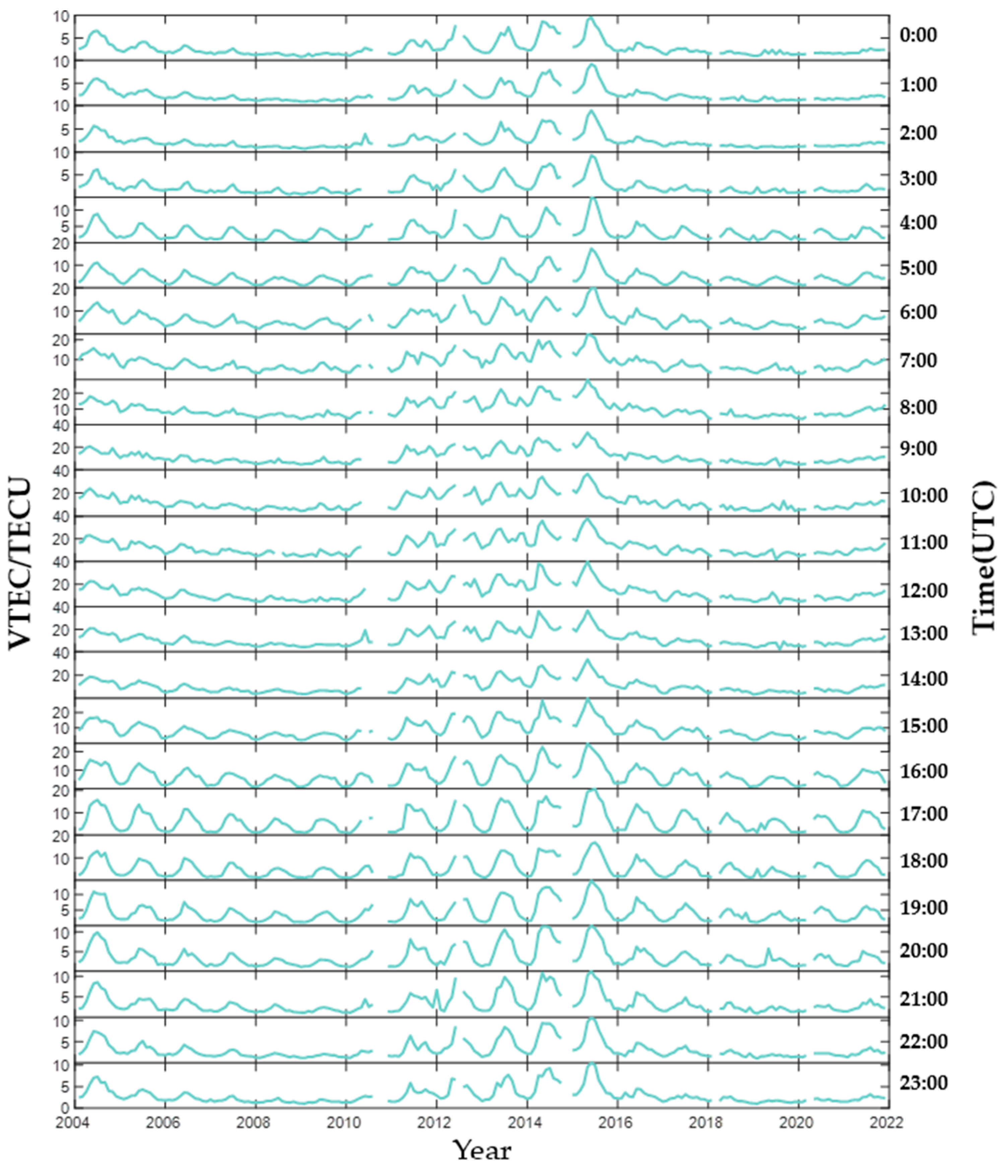
Figure 1. VTEC data curve for 24 h from 2004 to 2022 in Athens, Greece.
Remotesensing 15 02953 g001
Figure 2. Comparison between original and filtered TEC data.
Remotesensing 15 02953 g002
Figure 3. The curve diagram of TEC and solar activity parameters: (a) the curve diagram of filtered TEC data and F10.7 data; (b) the curve diagram of filtered TEC data and SSN data.
Remotesensing 15 02953 g003
Figure 4. Data flow diagram of the MMAdapGA-BP-NN prediction model.
Remotesensing 15 02953 g004
Figure 5. Schematic structure of the neural network, which is used in MMAdapGA-BP-NN.
Remotesensing 15 02953 g005
Figure 6. (a) The flowchart of BP-NN; (b) the flowchart of MMAdapGA-BP-NN.
Remotesensing 15 02953 g006
Figure 7. In the high solar activity year (2015), the scatter diagram and normal distribution diagram of the performance indicators of BP-NN, GA-BP-NN, and MMAdapGA-BP-NN after running 50 times: (a) the scatter diagram of the performance indicators of BP-NN, GA-BP-NN, and MMAdapGA-BP-NN running 50 times; (b) the normal distribution diagram of iteration times when the three models running 50 times; (c) the normal distribution diagram of RMSE when the three models running 50 times; and (d) the normal distribution diagram of ρ when the three models running 50 times.
Remotesensing 15 02953 g007
Figure 8. In the low solar activity year (2020), the scatter diagram and normal distribution diagram of the performance indicators of BP-NN, GA-BP-NN, and MMAdapGA-BP-NN running 50 times: (a) the scatter diagram of the performance indicators of BP-NN, GA-BP-NN, and MMAdapGA-BP-NN running 50 times; (b) the normal distribution diagram of iteration times when the three models running 50 times; (c) the normal distribution diagram of RMSE when the three models running for 50 times; (d) the normal distribution diagram of ρ when the three models running 50 times.
Remotesensing 15 02953 g008
Figure 9. Actual observed TEC data predicted TEC data and prediction error with IRI-2020, SML-F10.7, SML-SSN, BP-NN, GA-BP-NN, and MMAdapGA-BP-NN in a high solar activity year (2015) and low solar activity year (2020): (a) predicted TEC data of each model and actual observed TEC data in a high solar activity year (2015); (b) prediction error of each model in a high solar activity year (2015); (c) predicted TEC data of each model and actual observed TEC data in low solar activity year (2020); (d) prediction error of each model in a low solar activity year (2020).
Remotesensing 15 02953 g009
Figure 10. (ad) are the variation curves of monthly performance indicators (MAE, MRE, RMSE, and ρ of IRI-2020, SML-F10.7, SML-SSN, BP-NN, GA-BP-NN, and MMAdapGA-BP-NN in a high solar activity year (2015); (eh) are the variation curves of monthly performance indicators of the six models in a low solar activity year (2020); (fl) are the variation curves of monthly performance indicators of the average of two years of data.
Remotesensing 15 02953 g010
Figure 11. The deviation of TEC forecast data in daytime and night from MMAdapGA-BP-NN in a high solar activity year (2015) and low solar activity year (2020): (a) Prediction error stem of daytime and night in a high solar activity year (2015); (b) Prediction error stem of daytime and night in a low solar activity year (2020).
Remotesensing 15 02953 g011
Figure 12. (ad) are the performance indicators of MMAdapGA-BP-NN during daytime and night in a high solar activity year (2015) (average of 50 run results); (eh) are the performance indicators curve of MMAdapGA-BP-NN during daytime and night in a low solar activity year (2020) (average of 50 run results).
Remotesensing 15 02953 g012
Figure 13. The absolute error of predicted TEC and geomagnetic storm days bar graph: (a) The absolute error of predicted TEC and geomagnetic storm days in high solar activity years (2015); (b) The absolute error of predicted TEC and geomagnetic storm days in low solar activity years (2020).
Remotesensing 15 02953 g013
Table 1. Performances of each model in a high solar activity year (2015) and a low solar activity year (2020).
YearPerformance IRI-2020SML-F10.7SML-SSNBP-NNGA-BP-NNMMAdapGA-BP-NN
High Solar Activity Year (2015)MAE/TECU3.713.543.632.742.112.03
MRE/%34.0031.3331.5620.1416.7514.53
RMSE/TECU5.955.345.353.993.512.84
ρ0.750.790.770.820.850.91
Low Solar Activity Year (2020)MAE/TECU1.921.511.560.410.340.28
MRE/%18.2316.1216.246.045.273.54
RMSE/TECU3.052.872.961.121.030.85
ρ0.780.810.790.820.870.94
Mean ValueMAE/TECU2.822.562.601.581.231.16
MRE/%28.1223.8423.7919.0916.0113.54
RMSE/TECU4.624.344.313.062.761.94
ρ0.760.800.790.840.880.92
Table 2. Performance indices of MMAdapGA-BP-NN during daytime and night in a high solar activity year (2015) and low solar activity year (2020).
YearMAE/TECUMRE/%RMSE/TECUρ
High Solar Activity Year (2015)daytime2.4519.753.650.82
night1.3410.212.350.94
Low Solar Activity Year (2020)daytime0.375.421.040.90
night0.192.130.630.97
Table 3. The qualitative expression of geomagnetic storm intensity.
A p Geomagnetic Activity
>100Severe Storm
50~99Major Storm
30~49Minor Storm
16~29Active
8~15Unsettled
0~7Quiet
Disclaimer/Publisher’s Note: The statements, opinions and data contained in all publications are solely those of the individual author(s) and contributor(s) and not of MDPI and/or the editor(s). MDPI and/or the editor(s) disclaim responsibility for any injury to people or property resulting from any ideas, methods, instructions or products referred to in the content.