
Retrieving Atmospheric Gas Profiles Using FY-3E/HIRAS-II Infrared Hyperspectral Data by Neural Network Approach


Abstract
1. Introduction
2. Materials and Methods
2.1. Datasets
2.1.1. FY-3E/HIRAS-II
2.1.2. ERA5 and EAC4 Reanalysis Data
2.1.3. WACCM Forecast Data
2.1.4. GFS Forecast Data
2.1.5. AIRS Product Data
2.1.6. IASI Product Data
2.2. Data Preprocessing
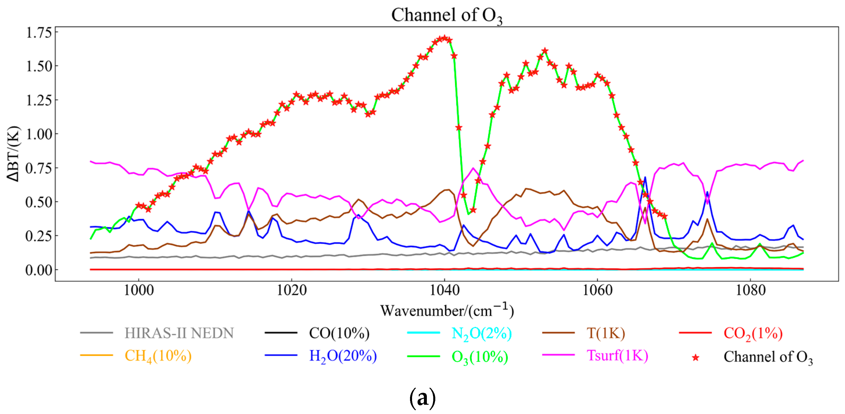
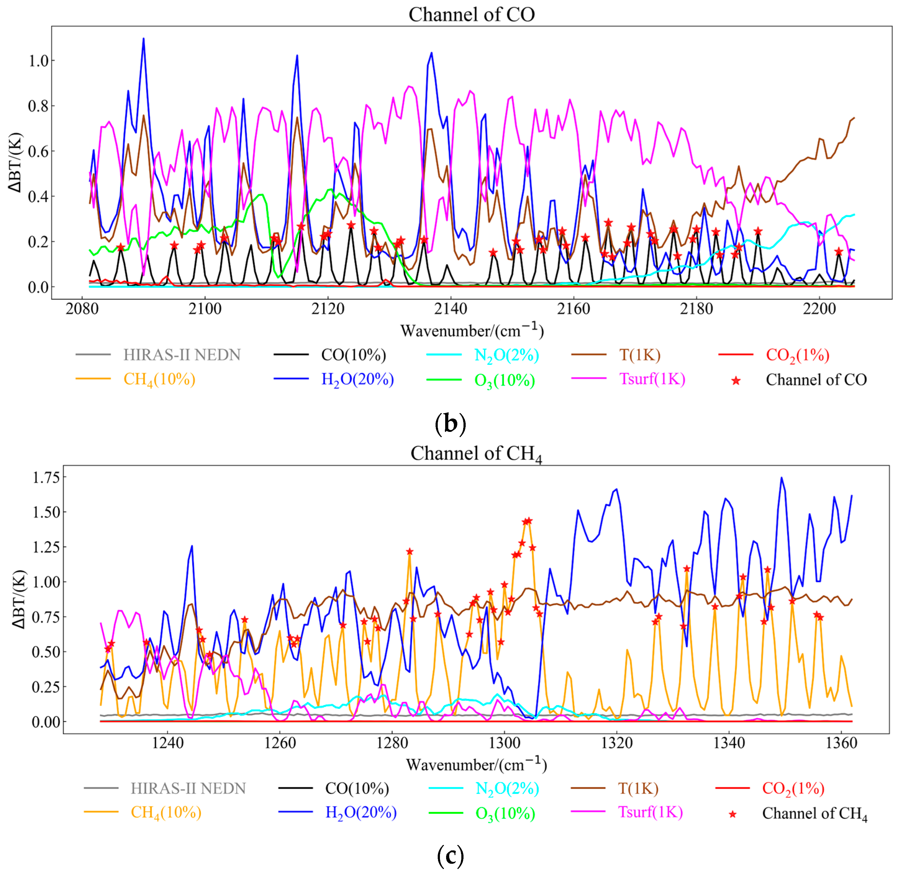
2.3. Channel Selection
2.4. Neural Network Model and Experimental Process
- (1)
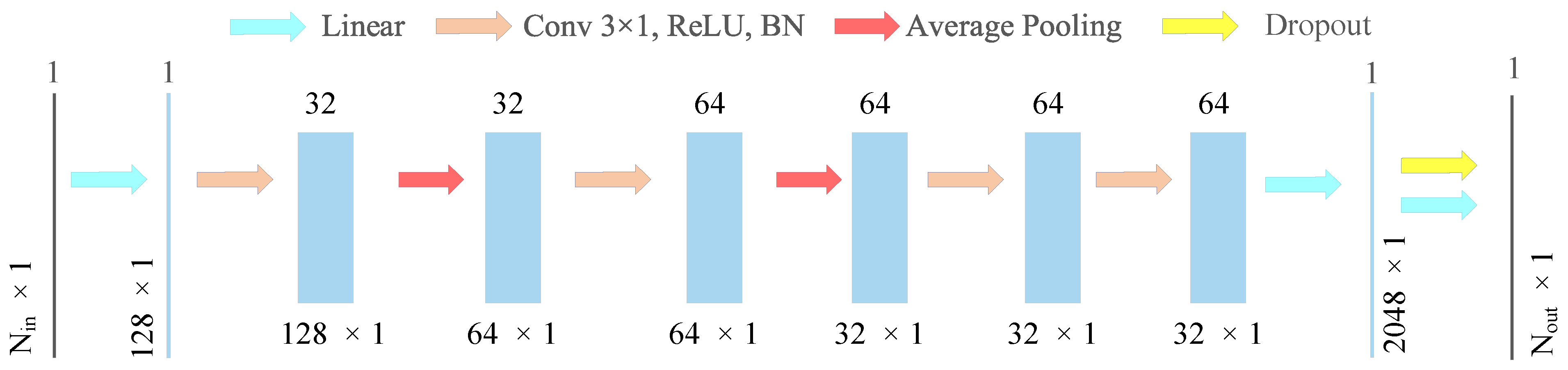
- CNN Model
- (2)
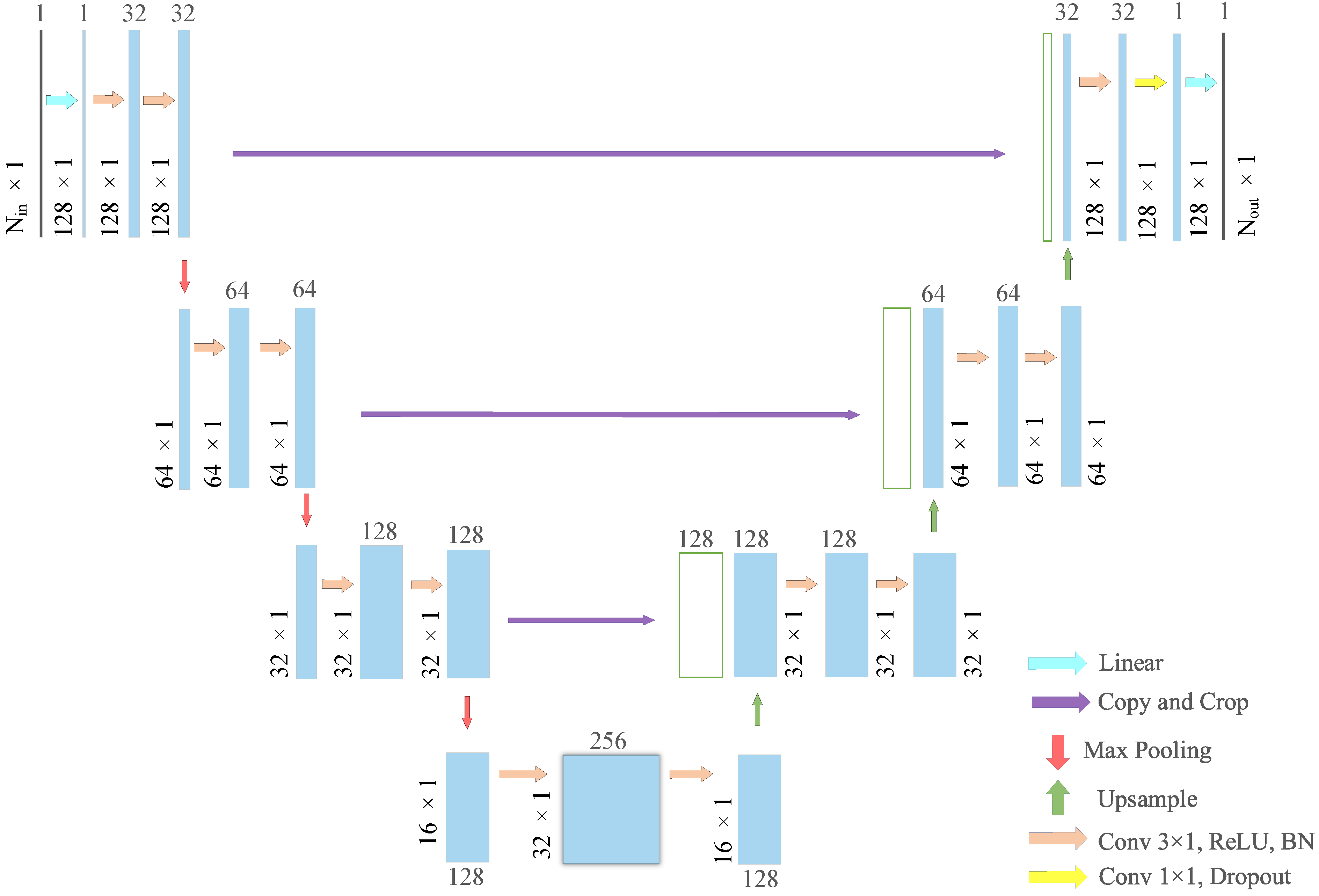
- UNET Network Model
3. Result
3.1. Analytical Method
3.2. Evaluation of Model Training and Test
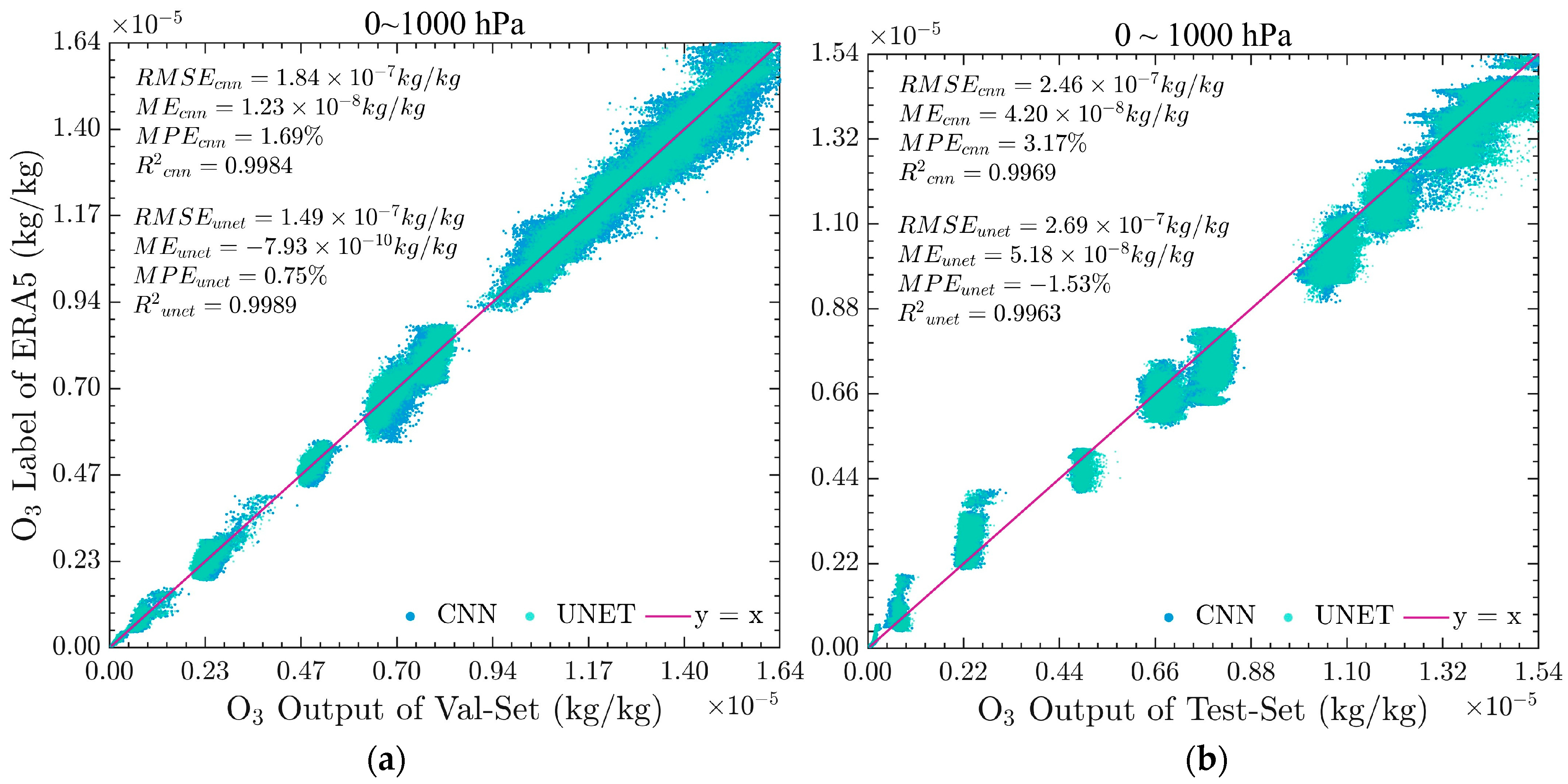
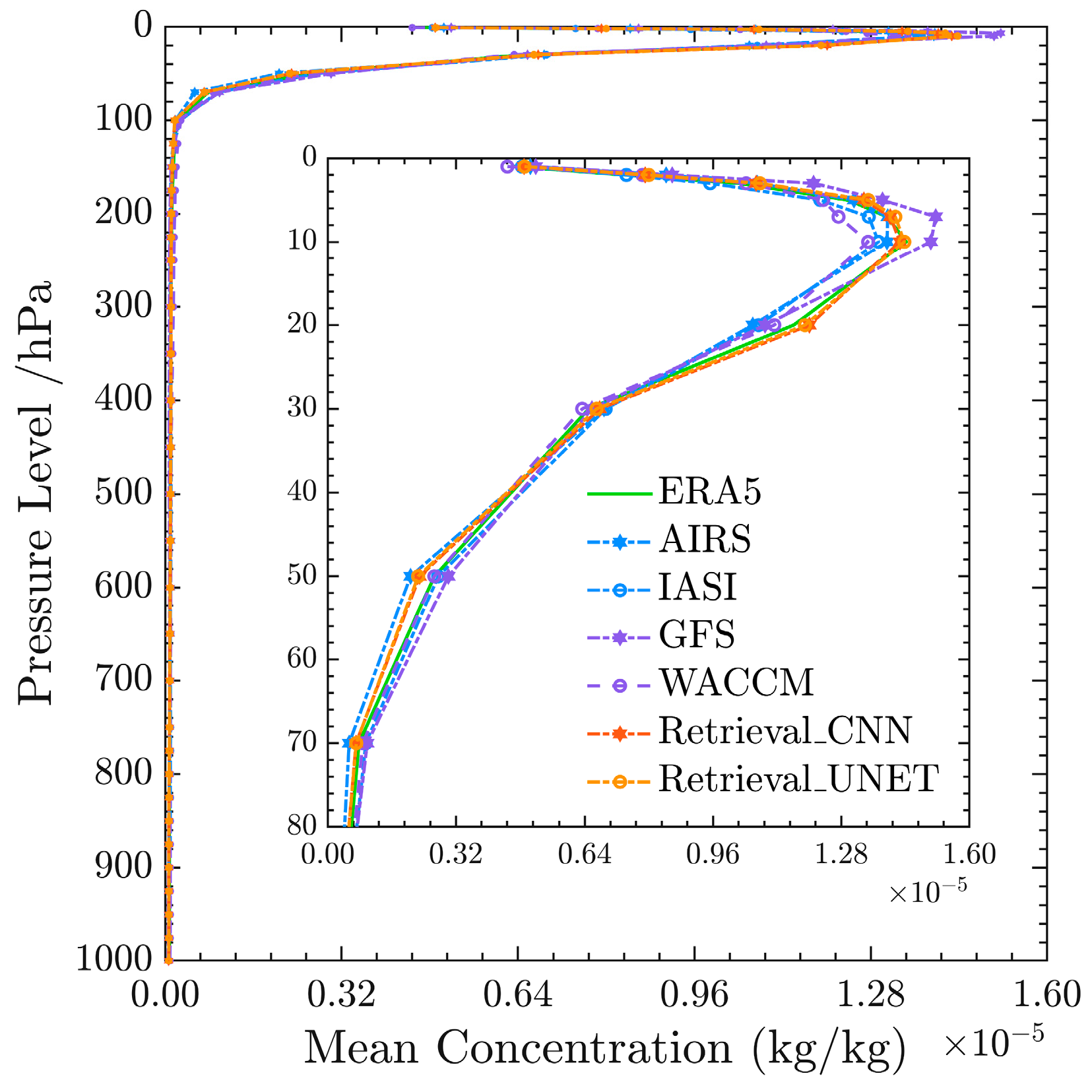
3.3. Analysis of O3 Retrieval Results
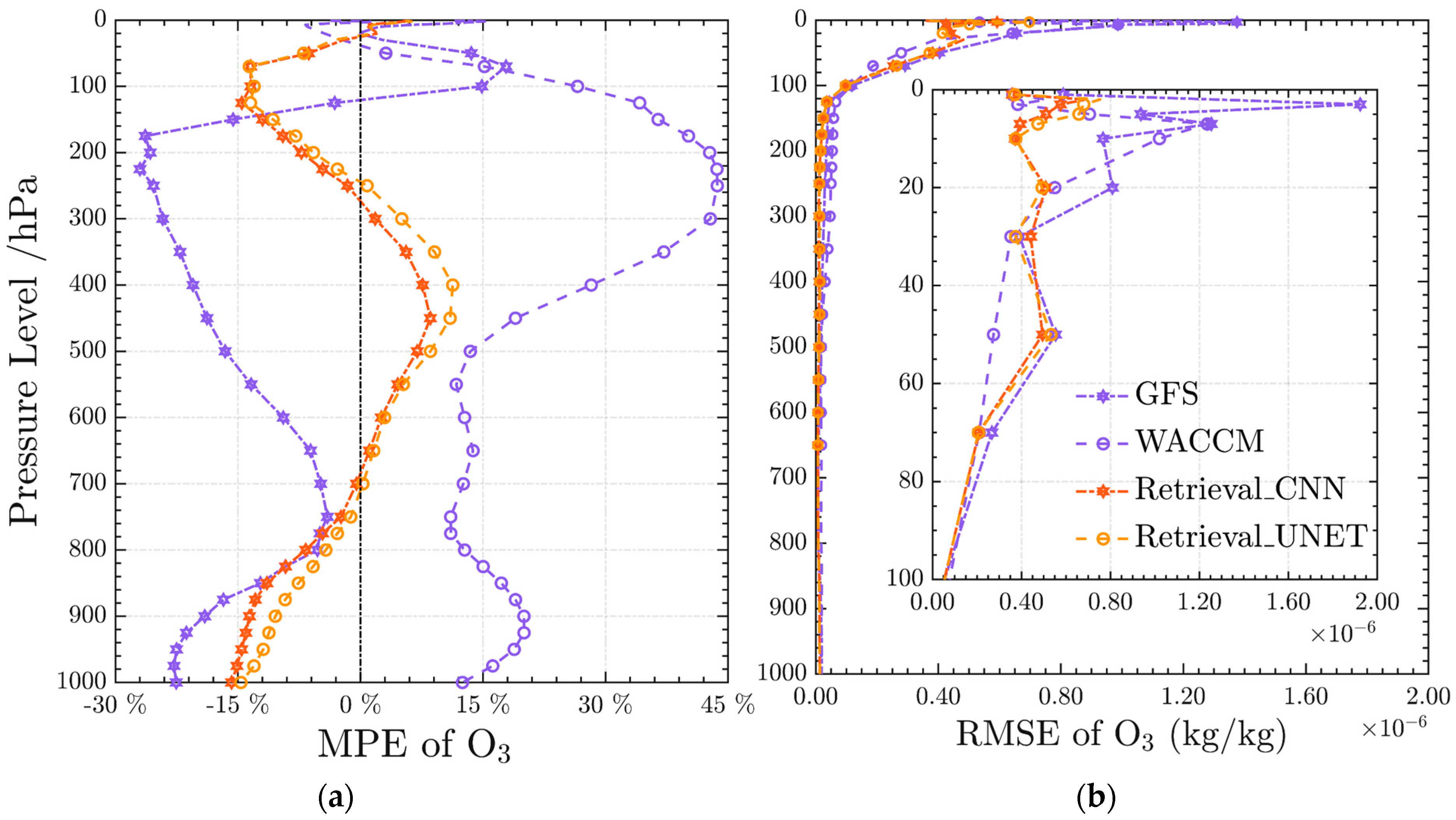
3.3.1. Comparison of O3 between Retrieval Results and Forecast Data
3.3.2. Comparison of O3 between Retrieval Results and Similar Satellite Products
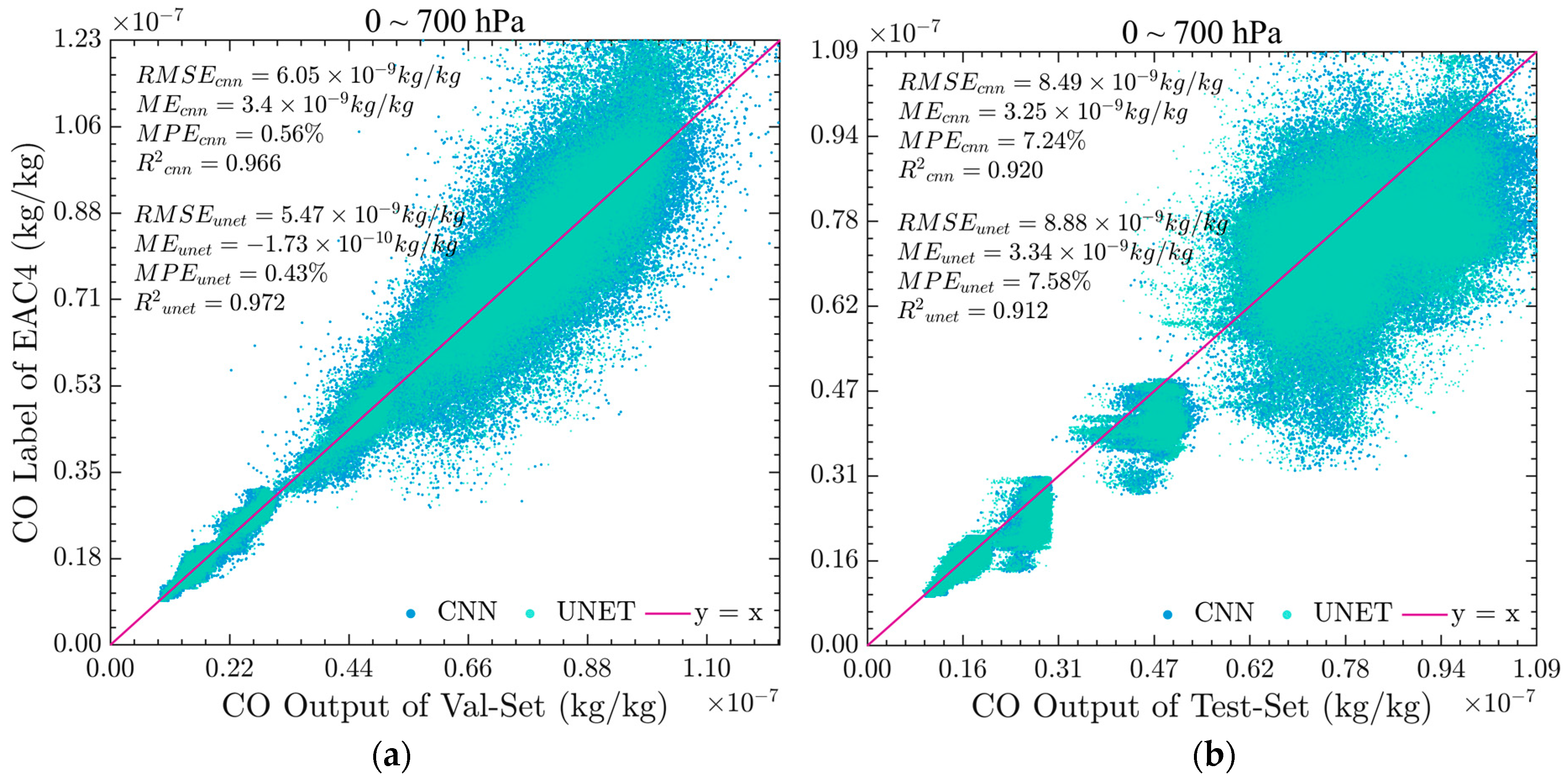
3.4. Analysis of CO Retrieval Results
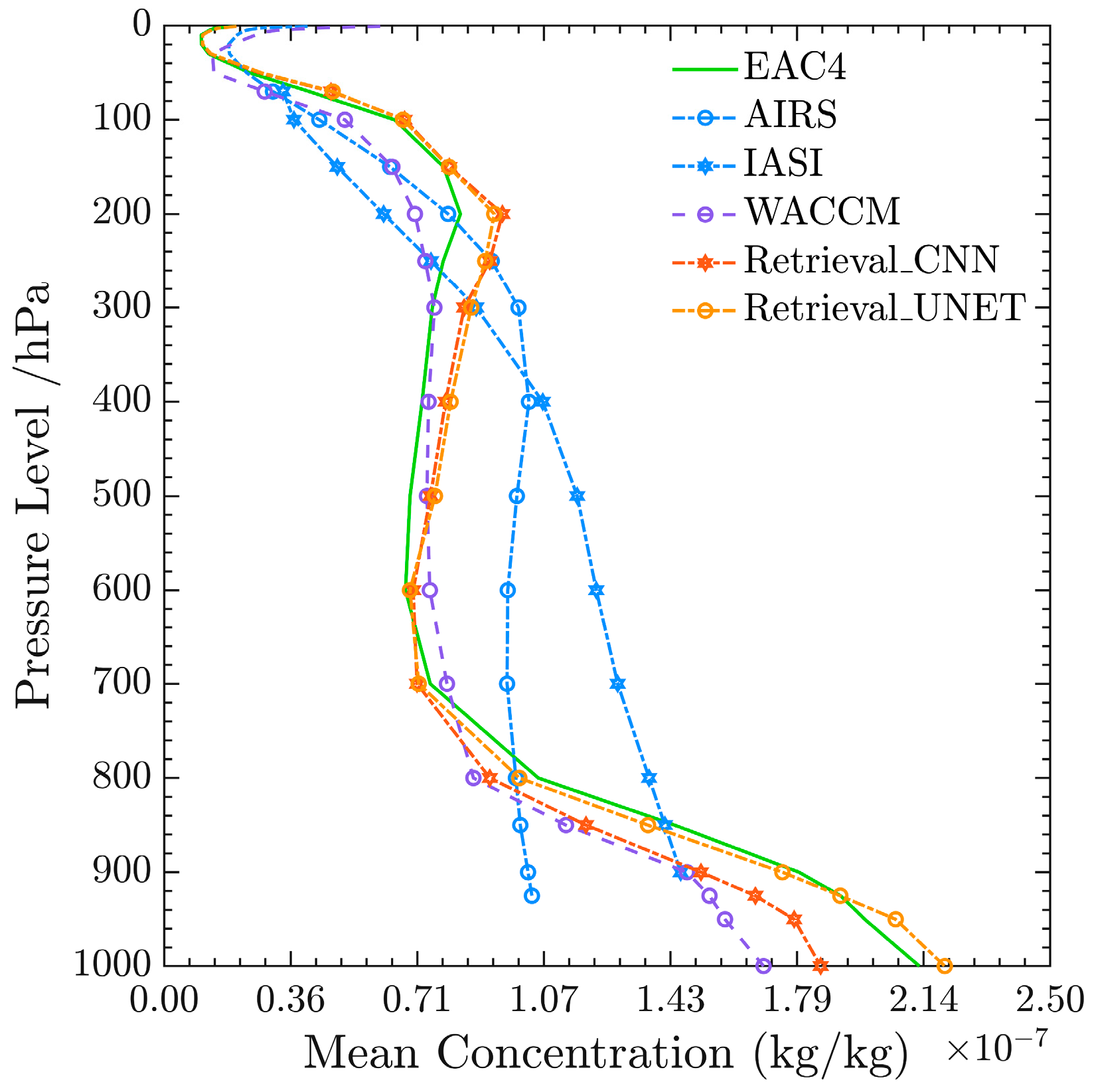
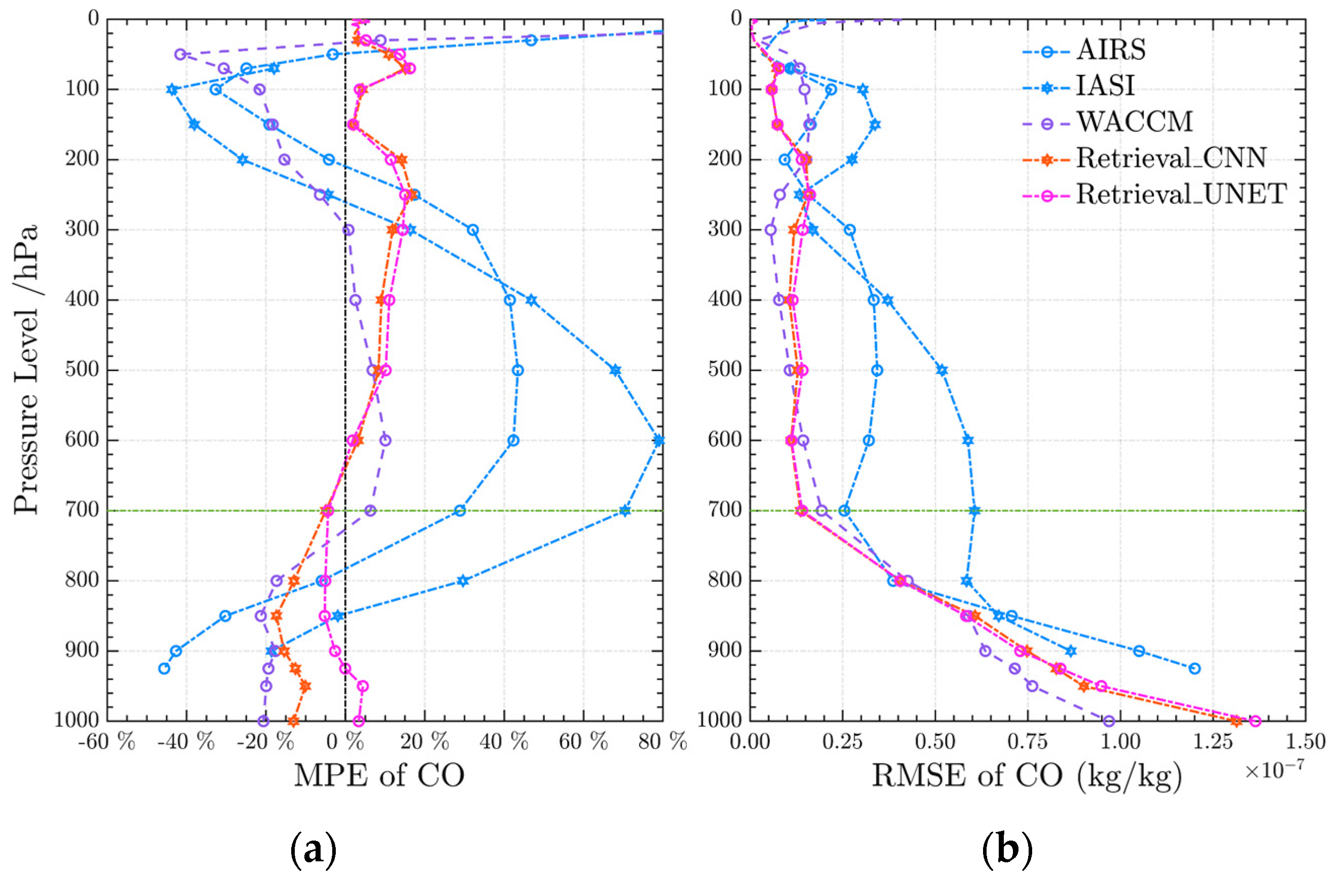
3.4.1. Comparison of CO between Retrieval Results and Forecast Data
3.4.2. Comparison of CO between Retrieval Results and Similar Satellite Products
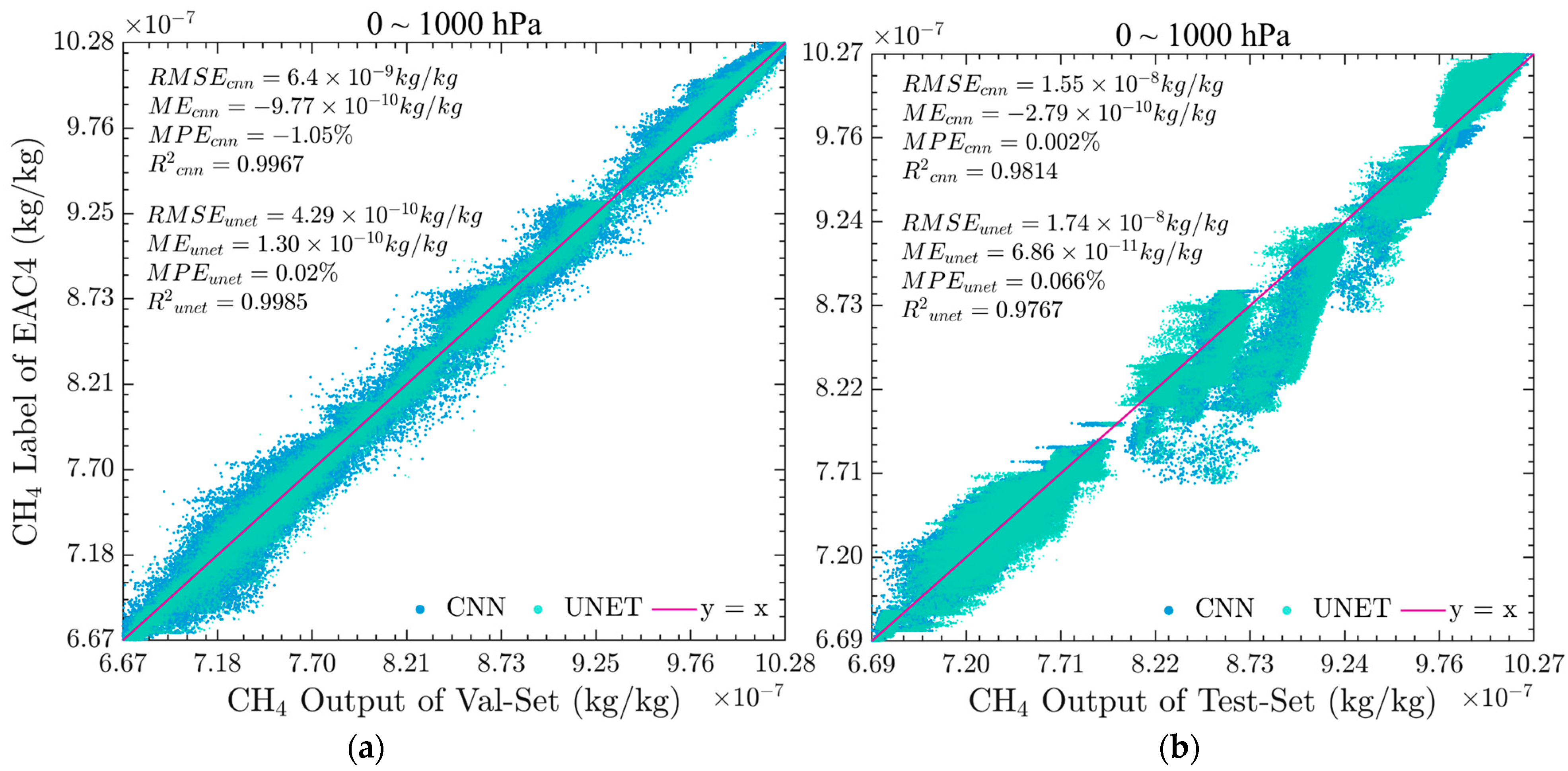
3.5. Analysis of CH4 Retrieval Results
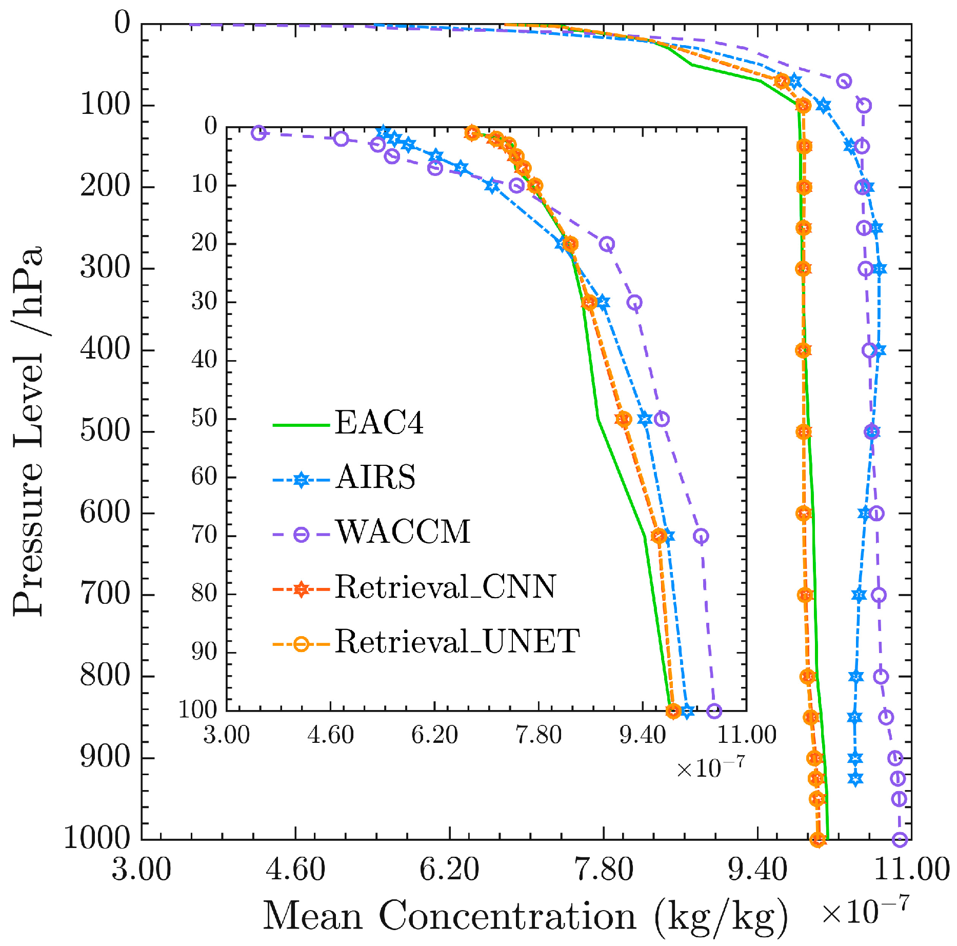
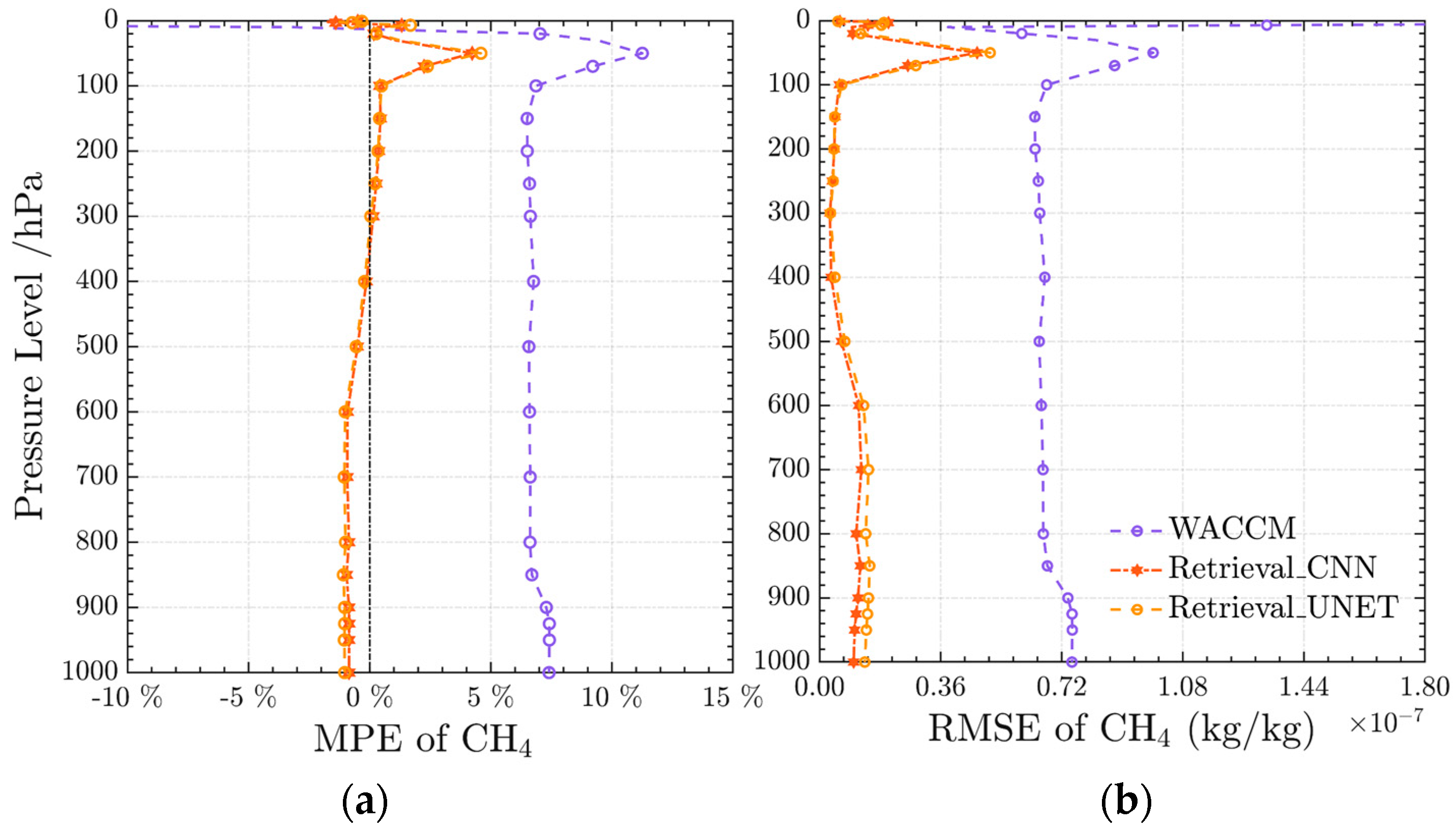
3.5.1. Comparison of CH4 between Retrieval Results and Forecast Data
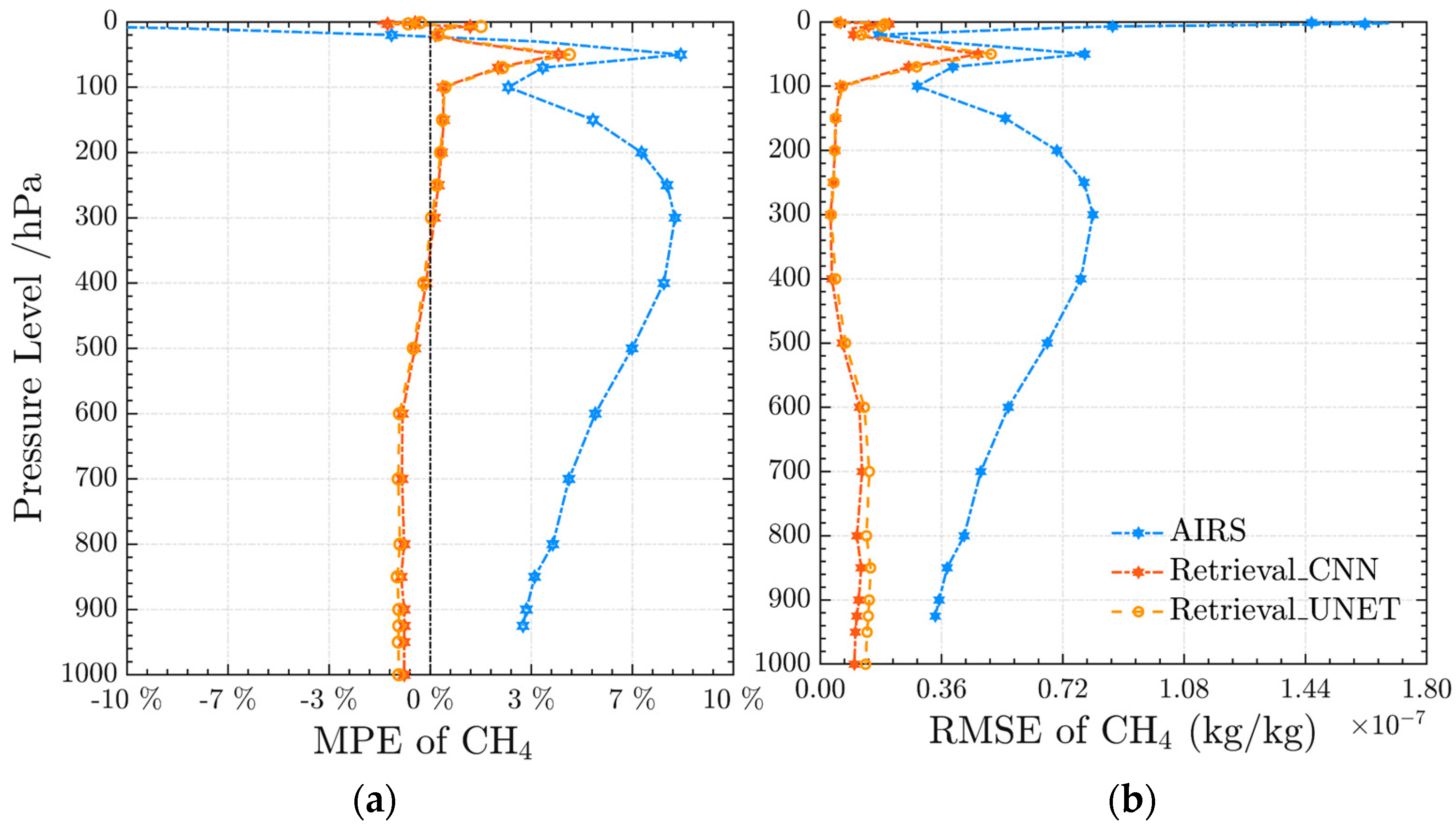
3.5.2. Comparison of CH4 between Retrieval Results and Similar Satellite Products
4. Discussion
5. Conclusions
Author Contributions
Funding
Data Availability Statement
Acknowledgments
Conflicts of Interest
Appendix A

| Count | Channels (cm−1) | |||||||
|---|---|---|---|---|---|---|---|---|
| O3 Channels | 96 | 1004.375 (569) | 1005.000 (570) | 1005.625 (571) | 1006.250 (572) | 1006.875 (573) | 1007.500 (574) | 1008.125 (575) |
| 1008.750 (576) | 1009.375 (577) | 1010.000 (578) | 1010.625 (579) | 1011.250 (580) | 1011.875 (581) | 1012.500 (582) | ||
| 1013.125 (583) | 1013.750 (584) | 1014.375 (585) | 1015.000 (586) | 1015.625 (587) | 1016.250 (588) | 1016.875 (589) | ||
| 1017.500 (590) | 1018.125 (591) | 1018.750 (592) | 1019.375 (593) | 1020.000 (594) | 1020.625 (595) | 1021.250 (596) | ||
| 1021.875 (597) | 1022.500 (598) | 1023.125 (599) | 1023.750 (600) | 1024.375 (601) | 1025.000 (602) | 1025.625 (603) | ||
| 1026.250 (604) | 1026.875 (605) | 1027.500 (606) | 1028.125 (607) | 1028.750 (608) | 1029.375 (609) | 1030.000 (610) | ||
| 1030.625 (611) | 1031.250 (612) | 1031.875 (613) | 1032.500 (614) | 1033.125 (615) | 1033.750 (616) | 1034.375 (617) | ||
| 1035.000 (618) | 1035.625 (619) | 1036.250 (620) | 1036.875 (621) | 1037.500 (622) | 1038.125 (623) | 1038.750 (624) | ||
| 1039.375 (625) | 1040.000 (626) | 1040.625 (627) | 1041.250 (628) | 1041.875 (629) | 1044.375 (633) | 1045.000 (634) | ||
| 1045.625 (635) | 1046.250 (636) | 1046.875 (637) | 1047.500 (638) | 1048.125 (639) | 1048.750 (640) | 1049.375 (641) | ||
| 1050.000 (642) | 1050.625 (643) | 1051.250 (644) | 1051.875 (645) | 1052.500 (646) | 1053.125 (647) | 1053.750 (648) | ||
| 1054.375 (649) | 1055.000 (650) | 1055.625 (651) | 1056.250 (652) | 1056.875 (653) | 1057.500 (654) | 1058.125 (655) | ||
| 1058.750 (656) | 1059.375 (657) | 1060.000 (658) | 1060.625 (659) | 1061.250 (660) | 1061.875 (661) | 1062.500 (662) | ||
| 1063.125 (663) | 1063.750 (664) | 1064.375 (665) | 1065.000 (666) | 1065.625 (667) | ||||
| CO Channels | 76 | 2081.875 (2301) | 2082.500 (2302) | 2085.625 (2307) | 2086.250 (2308) | 2086.875 (2309) | 2090.000 (2314) | 2090.625 (2315) |
| 2094.375 (2321) | 2095.000 (2322) | 2098.750 (2328) | 2099.375 (2329) | 2102.500 (2334) | 2103.125 (2335) | 2103.750 (2336) | ||
| 2106.875 (2341) | 2107.500 (2342) | 2108.125 (2343) | 2110.625 (2347) | 2111.250 (2348) | 2111.875 (2349) | 2115.000 (2354) | ||
| 2115.625 (2355) | 2116.250 (2356) | 2119.375 (2361) | 2120.000 (2362) | 2120.625 (2363) | 2123.125 (2367) | 2123.750 (2368) | ||
| 2124.375 (2369) | 2126.875 (2373) | 2127.500 (2374) | 2128.125 (2375) | 2131.250 (2380) | 2131.875 (2381) | 2135.000 (2386) | ||
| 2135.625 (2387) | 2136.250 (2388) | 2139.375 (2393) | 2146.875 (2405) | 2147.500 (2406) | 2150.625 (2411) | 2151.250 (2412) | ||
| 2153.750 (2416) | 2154.375 (2417) | 2155.000 (2418) | 2157.500 (2422) | 2158.125 (2423) | 2158.750 (2424) | 2161.250 (2428) | ||
| 2161.875 (2429) | 2162.500 (2430) | 2165.000 (2434) | 2165.625 (2435) | 2166.250 (2436) | 2168.750(2440) | 2169.375 (2441) | ||
| 2170.000 (2442) | 2172.500 (2446) | 2173.125 (2447) | 2175.625 (2451) | 2176.250 (2452) | 2176.875 (2453) | 2179.375 (2457) | ||
| 2180.000 (2458) | 2180.625 (2459) | 2182.500 (2462) | 2183.125 (2463) | 2183.750 (2464) | 2186.250 (2468) | 2186.875 (2469) | ||
| 2189.375 (2473) | 2190.000 (2474) | 2190.625 (2475) | 2193.125 (2479) | 2203.125 (2495) | 2203.750 (2496) | |||
| CH4 Channels | 150 | 1228.750 (932) | 1229.375 (933) | 1230.000 (934) | 1230.625 (935) | 1233.750 (940) | 1235.625 (943) | 1236.250 (944) |
| 1236.875 (945) | 1237.500 (946) | 1238.125 (947) | 1238.750 (948) | 1240.625 (951) | 1241.250 (952) | 1241.875 (953) | ||
| 1242.500 (954) | 1243.125 (955) | 1245.000 (958) | 1245.625 (959) | 1246.250 (960) | 1246.875 (961) | 1247.500 (962) | ||
| 1248.125 (963) | 1248.750 (964) | 1249.375 (965) | 1250.000 (966) | 1252.500 (970) | 1253.125 (971) | 1253.750 (972) | ||
| 1254.375 (973) | 1255.000 (974) | 1255.625 (975) | 1256.250 (976) | 1256.875 (977) | 1258.750 (980) | 1259.375 (981) | ||
| 1260.000 (982) | 1260.625 (983) | 1261.250 (984) | 1261.875 (985) | 1262.500 (986) | 1263.125 (987) | 1263.750 (988) | ||
| 1264.375 (989) | 1265.000 (990) | 1265.625 (991) | 1266.250 (992) | 1267.500 (994) | 1268.125 (995) | 1268.750 (996) | ||
| 1269.375 (997) | 1270.000 (998) | 1270.625 (999) | 1271.250 (1000) | 1271.875 (1001) | 1274.375 (1005) | 1275.000 (1006) | ||
| 1275.625 (1007) | 1276.250 (1008) | 1276.875 (1009) | 1277.500 (1010) | 1278.125 (1011) | 1281.250 (1016) | 1281.875 (1017) | ||
| 1282.500 (1018) | 1283.125 (1019) | 1283.750 (1020) | 1284.375 (1021) | 1286.875 (1025) | 1287.500 (1026) | 1288.125 (1027) | ||
| 1288.750 (1028) | 1289.375 (1029) | 1290.000 (1030) | 1291.875 (1033) | 1292.500 (1034) | 1293.125 (1035) | 1293.750 (1036) | ||
| 1294.375 (1037) | 1295.000 (1038) | 1295.625 (1039) | 1296.250 (1040) | 1296.875 (1041) | 1297.500 (1042) | 1298.125 (1043) | ||
| 1298.750 (1044) | 1299.375 (1045) | 1300.000 (1046) | 1300.625 (1047) | 1301.250 (1048) | 1301.875 (1049) | 1302.500 (1050) | ||
| 1303.125 (1051) | 1303.750 (1052) | 1304.375 (1053) | 1305.000 (1054) | 1305.625 (1055) | 1306.250 (1056) | 1306.875(1057) | ||
| 1307.500 (1058) | 1311.250 (1064) | 1311.875 (1065) | 1316.875 (1073) | 1321.250 (1080) | 1321.875 (1081) | 1322.500 (1082) | ||
| 1323.125 (1083) | 1323.750 (1084) | 1324.375 (1085) | 1326.250 (1088) | 1326.875 (1089) | 1327.500 (1090) | 1328.125 (1091) | ||
| 1328.750 (1092) | 1331.250 (1096) | 1331.875 (1097) | 1332.500 (1098) | 1333.125 (1099) | 1333.750 (1100) | 1334.375 (1101) | ||
| 1336.250 (1104) | 1336.875 (1105) | 1337.500 (1106) | 1338.125 (1107) | 1341.250 (1112) | 1341.875 (1113) | 1342.500 (1114) | ||
| 1343.125 (1115) | 1343.750 (1116) | 1345.625 (1119) | 1346.250 (1120) | 1346.875 (1121) | 1347.500 (1122) | 1348.125 (1123) | ||
| 1348.750 (1124) | 1350.625 (1127) | 1351.250 (1128) | 1351.875 (1129) | 1352.500 (1130) | 1353.125 (1131) | 1353.750 (1132) | ||
| 1355.000 (1134) | 1355.625 (1135) | 1356.250 (1136) | 1356.875 (1137) | 1357.500 (1138) | 1358.125 (1139) | 1359.375 (1141) | ||
| 1360.000 (1142) | 1360.625 (1143) | 1361.250 (1144) | ||||||
References
- Zhang, X.; Wang, F.; Wang, W.; Huang, F.; Chen, B.; Gao, L.; Wang, S.; Yan, H.; Ye, H.; Si, F.; et al. Development and Application of Satellite Remote Sensing for Atmospheric Compositions in China. Adv. Meteorol. Sci. Technol. 2022, 12, 64–73. [Google Scholar] [CrossRef]
- Liang, P.; Niu, S.J. A Comparison of Total Column Ozone Values Derived from AIRS, TOVS and TOMS. J. Remote Sens. 2008, 30, 196–203. [Google Scholar] [CrossRef]
- Winterstein, F.; Tanalski, F.; Jckel, P.; Dameris, M.; Ponater, M. Implication of Strongly Increased Atmospheric Methane Concentrations for Chemistry–Climate Connections. Atmos. Chem. Phys. 2019, 19, 7151–7163. [Google Scholar] [CrossRef]
- Sierk, B.; Richter, A.; Rozanov, A.; Savigny, C.V.; Schmoltner, A.M.; Buchwitz, M.; Bovensmann, H.; Burrows, J.P. Retrieval and Monitoring of Atmospheric Trace Gas Concentrations in Nadir and Limb Geometry Using the Space-Borne Sciamachy Instrument. Env. Monit Assess. 2006, 120, 65–77. [Google Scholar] [CrossRef] [PubMed]
- Clerbaux, C.; Boynard, A.; Clarisse, L.; George, M.; Hadji-Lazaro, J.; Herbin, H.; Hurtmans, D.; Pommier, M.; Razavi, A.; Turquety, S.; et al. Monitoring of Atmospheric Composition Using the Thermal Infrared IASI/MetOp Sounder. Atmos. Chem. Phys. 2009, 9, 6041–6054. [Google Scholar] [CrossRef]
- Chengli, Q.; Mingjian, G.; Xiuqing, H.; Chunqiang, W. FY-3 Satellite Infrared High Spectral Sounding Technique and Potential Application. Adv. Meteorol. Sci. Technol. 2016, 6, 88–93. [Google Scholar]
- David, M.; Ibrahim, M.H.; Idrus, S.M.; Ngajikin, N.H.; Azmi, A.I.; En Marcus, T.C. Optical Path Length, Temperature, and Wavelength Effects Simulation on Ozone Gas Absorption Cross Sections towards Green Communications. J. Electron. Sci. Technol. 2016, 14, 199–204. [Google Scholar] [CrossRef]
- Liou, K.N. An Introduction to Atmospheric Radiation; China Meteorological Press: Beijing, China, 2004. [Google Scholar]
- Beibei, Z.; Ning, W.; Weiyuan, Y.; Lingling, M. Channel selection for carbon monoxide retrievals based on ultraspectral thermal infrared data. J. Infrared Millim. Waves 2021, 40, 391–399. [Google Scholar]
- Han, Y.; Revercomb, H.; Cromp, M.; Gu, D.; Johnson, D.; Mooney, D.; Scott, D.; Strow, L.; Bingham, G.; Borg, L.; et al. Suomi NPP CrIS Measurements, Sensor Data Record Algorithm, Calibration and Validation Activities, and Record Data Quality. J. Geophys. Res. Atmos. 2013, 118, 12–734. [Google Scholar] [CrossRef]
- Hilton, F.; Armante, R.; August, T.; Barnet, C.; Zhou, D. Hyperspectral Earth Observation from IASI. Bull. Am. Meteorol. Soc. 2012, 93, 347–370. [Google Scholar] [CrossRef]
- Chahine, M.T.; Pagano, T.S.; Aumann, H.H.; Atlas, R.; Barnet, C.; Blaisdell, J.; Chen, L.; Divakarla, M.; Fetzer, E.J.; Goldberg, M.; et al. AIRS: Improving Weather Forecasting and Providing New Data on Greenhouse Gases. Am. Meteorol. Soc. 2006, 87, 911–926. [Google Scholar] [CrossRef]
- Nalli, N.R.; Tan, C.; Warner, J.; Divakarla, M.; Gambacorta, A.; Wilson, M.; Zhu, T.; Wang, T.; Wei, Z.; Pryor, K.; et al. Validation of Carbon Trace Gas Profile Retrievals from the NOAA-Unique Combined Atmospheric Processing System for the Cross-Track Infrared Sounder. Remote Sens. 2020, 12, 3245. [Google Scholar] [CrossRef]
- De Wachter, E.; Barret, B.; Le Flochmoën, E.; Pavelin, E.; Matricardi, M.; Clerbaux, C.; Hadji-Lazaro, J.; George, M.; Hurtmans, D.; Coheur, P.F.; et al. Retrieval of MetOp-A/IASI CO Profiles and Validation with MOZAIC Data. Atmos. Meas. Tech. 2012, 5, 2843–2857. [Google Scholar] [CrossRef]
- Serio, C.; Blasi, M.G.; Liuzzi, G.; Masiello, G.; Venafra, S. Using the Full IASI Spectrum for the Physical Retrieval of Temperature, H2O, HDO, O-3, Minor and Trace Gases. In Proceedings of the Radiation Processes in the Atmosphere and Ocean; Davies, R., Egli, L., Schmutz, W., Eds.; Amer Inst Physics: Melville, NY, USA, 2017; Volume 1810, p. 060004. [Google Scholar]
- Nalli, N.R.; Gambacorta, A.; Liu, Q.; Tan, C.; Iturbide-Sanchez, F.; Barnet, C.D.; Joseph, E.; Morris, V.R.; Oyola, M.; Smith, J.W. Validation of Atmospheric Profile Retrievals from the SNPP NOAA-Unique Combined Atmospheric Processing System. Part 2: Ozone. IEEE Trans. Geosci. Remote Sens. 2018, 56, 598–607. [Google Scholar] [CrossRef]
- Rodgers, C.D. Inverse Methods for Atmospheric Sounding-Theory and Practice; World Scientific: Singapore, 2000. [Google Scholar] [CrossRef]
- Cyril, C.; Alain, C.; Scott, N.A. AIRS Channel Selection for CO2 and Other Trace-gas Retrievals. Q. J. R. Meteorol. Soc. 2010, 129, 2719–2740. [Google Scholar] [CrossRef]
- Zong, X. Inversion accuracy and spectral channel evaluation of atmospheric polluted gases of atmospheric infrared radiation ultra-high detector under limb sounding. Acta Sci. Circumstantiae 2020, 40, 1410–1421. [Google Scholar] [CrossRef]
- Li, S.; Hu, H.; Fang, C.; Wang, S.; Xun, S.; He, B.; Wu, W.; Huo, Y. Hyperspectral Infrared Atmospheric Sounder (HIRAS) Atmospheric Sounding System. Remote Sens. 2022, 14, 3882. [Google Scholar] [CrossRef]
- Zhang, C.; Gu, M.; Hu, Y.; Huang, P.; Yang, T.; Huang, S.; Yang, C.; Shao, C. A Study on the Retrieval of Temperature and Humidity Profiles Based on FY-3D/HIRAS Infrared Hyperspectral Data. Remote Sens. 2021, 13, 2157. [Google Scholar] [CrossRef]
- Wang, Y. Research on Temperature/Pressure and Ozone Retrieval Algorithm Based on Atmospheric Infrared Ultraspectral Spectrometer. Master’s Thesis, Institute of Remote Sensing and Digital Earth, Chinese Academy of Sciences, Beijing, China, 2017. [Google Scholar]
- Wang, T. Retrieval of Atmospheric CO Vertical Profiles on CrIS IR Hyperspectral Satellite Data. Master’s Thesis, Chinese Academy of Sciences, Beijing, China, 2015. [Google Scholar]
- Noël, S.; Bramstedt, K.; Hilker, M.; Liebing, P.; Plieninger, J.; Reuter, M.; Rozanov, A.; Sioris, C.E.; Bovensmann, H.; Burrows, J.P. Stratospheric CH4 and CO2 Profiles Derived from SCIAMACHY Solar Occultation Measurements. Atmos. Meas. Tech. 2016, 8, 11467–11511. [Google Scholar] [CrossRef]
- Zhang, Y.; Chen, L.; Tao, J.; Su, L.; Yu, C.; Fan, M. Retrieval of Methane Profiles from Spaceborne Hyperspectral Infrared Observations. J. Remote Sens. 2012, 16, 232–247. [Google Scholar]
- Zhou, M.; Shu, J.; Song, C.; Gao, W. Sensitivity Studies for Atmospheric Carbon Dioxide Retrieval from Atmospheric Infrared Sounder Observations. J. Appl. Remote Sens. 2014, 8, 083697. [Google Scholar] [CrossRef]
- Song, C.; Shu, J.; Zhou, M.; Gao, W. Sensitivity Studies of High-Precision Methane Column Concentration Inversion Using a Line-by-Line Radiative Transfer Model. Front. Earth Sci. 2013, 7, 46. [Google Scholar] [CrossRef]
- Deng, J.; Liu, Y.; Yang, D.; Cai, Z. CH4 Retrieval from Hyperspectral Satellite Measurements in Short-Wave Infrared: Sensitivity Study and Preliminary Test with GOSAT Data. Chin. Sci. Bull. 2014, 59, 1499–1507. [Google Scholar] [CrossRef]
- Kolassa, J.; Gentine, P.; Prigent, C.; Aires, F.; Alemohammad, S.H. Soil Moisture Retrieval from AMSR-E and ASCAT Microwave Observation Synergy. Part 2: Product Evaluation. Remote Sens. Environ. 2017, 195, 202–217. [Google Scholar] [CrossRef]
- Zhang, X.; Guan, L.; Wang, Z.; Han, J. Retrieving Atmospheric Temperature Profiles Using Artificial Neural Network Approach. Meteorol. Mon. 2009, 35, 137–142. [Google Scholar]
- Liu, Y.; Guan, L. Study on the Inversion of Clear Sky Atmospheric Humidity Profiles with Artificial Neural Network. Meteorol. Mon. 2011, 37, 318–324. [Google Scholar]
- Huang, S. An Improved Method Combining CNN and 1D-Var for the Retrieval of Atmospheric Humidity Profiles from FY-4A/GIIRS Hyperspectral Data. Remote Sens. 2021, 13, 4737. [Google Scholar] [CrossRef]
- Shuhan, Y.; Li, G. Atmospheric temperature and humidity profile retrievals using a machine learning algorithm based on satellite-based infrared hyperspectral observations. Infrared Laser Eng. 2022, 51, 461–472. [Google Scholar]
- Xue, Q. Research on Retrieval Algorithm of All Sky Atmospheric Temperature and Humidity Profiles from the FY4A GIIRS. Ph.D. Thesis, Nanjing University of Information Science & Technology, Nanjing, China, 2022. [Google Scholar]
- Chowdhury, S.; Rubi, M.A.; Bijoy, M. Application of Artificial Neural Network for Predicting Agricultural Methane and CO2 Emissions in Bangladesh. In Proceedings of the 2021 12th International Conference on Computing Communication and Networking Technologies (ICCCNT), Kharagpur, India, 6–8 July 2021. [Google Scholar]
- Sayeed, A.; Choi, Y.; Eslami, E.; Lops, Y.; Roy, A.; Jung, J. Using a Deep Convolutional Neural Network to Predict 2017 Ozone Concentrations, 24 Hours in Advance. Neural Netw. 2020, 121, 396–408. [Google Scholar] [CrossRef] [PubMed]
- Zhang, X.; Zhang, Y.; Lu, X.; Bai, L.; Zhu, L. Estimation of Lower-Stratosphere-to-Troposphere Ozone Profile Using Long Short-Term Memory (LSTM). Remote Sens. 2021, 13, 1374. [Google Scholar] [CrossRef]
- Jarosawski, J. Improvement of the Umkehr Ozone Profile by the Neural Network Method: Analysis of the Belsk Umkehr Data. Int. J. Remote Sens. 2013, 34, 5541–5550. [Google Scholar] [CrossRef]
- Zhang, P.; Hu, X.; Lu, Q.; Zhu, A.; Lin, M.; Sun, L.; Chen, L.; Xu, N. FY-3E:The First Operational Meteorological Satellite Mission in an Early Morning Orbit. Adv. Atmos. Sci. 2022, 39, 1–8. [Google Scholar] [CrossRef]
- Yang, T.; Zhang, C.; Zuo, F.; Hu, Y.; Gu, M. Uncertainty analysis of inter-calibration collocation based on FY-3E spaceborne infrared observations. Infrared Laser Eng. 2022, 1–9. [Google Scholar]
- Tian-Hang, Y.; Ming-Jian, G.; Chun-Yuan, S.; Chun-Qiang, W.; Cheng-Li, Q.; Xiuqing, L. Nonlinearity correction of FY-3E HIRAS-II in pre-launch thermal vacuum calibration tests. J. Infrared Millim. Waves 2022, 41, 597–607. [Google Scholar] [CrossRef]
- Zhang, C.; Qi, C.; Yang, T.; Gu, M.; Zhang, P.; Lee, L.; Hu, X. Evaluation of FY-3E/HIRAS-II Radiometric Calibration Accuracy Based on OMB Analysis. Remote Sens. 2022, 14, 3222. [Google Scholar] [CrossRef]
- Chen, H.; Guan, L. Assessing FY-3E HIRAS-II Radiance Accuracy Using AHI and MERSI-LL. Remote Sens. 2022, 14, 4309. [Google Scholar] [CrossRef]
- Yang, T. Tropospheric Wind Field Measurement Based on Infrared Hyperspectral Observations. Ph.D. Thesis, Shanghai Institute of Technical Physics, University of Chinese Academy of Sciences, Shanghai, China, 2020. [Google Scholar]
- Ren, J. Study on the Atmospheric Temperature and Humidity Profiles of Satellite Remote Sensing Based on One-Dimensional Variational Algorithm. Master’s Thesis, Nanjing University of Information Science and Technology, Nanjing, China, 2018. [Google Scholar]
- Crevoisier, C.; Clerbaux, C.; Guidard, V.; Phulpin, T.; Armante, R.; Barret, B.; Camy-Peyret, C.; Chaboureau, J.P.; Coheur, P.F.; Crépeau, L.; et al. Towards IASI-New Generation (IASI-NG): Impact of Improved Spectral Resolution and Radiometric Noise on the Retrieval of Thermodynamic, Chemistry and Climate Variables. Atmos. Meas. Tech. 2014, 7, 4367–4385. [Google Scholar] [CrossRef]
- Luo, L.; Qiu, D.; Cui, L. Study on FY-4A/GIIRS infrared spectrum detection capability based on information content. J. Infrared Millim. Waves 2019, 38, 765–776. [Google Scholar]
- Shenfield, A.; Howarth, M. A Novel Deep Learning Model for the Detection and Identification of Rolling Element-Bearing Faults. Sensors 2020, 20, 5112. [Google Scholar] [CrossRef]
- Ying Huang; Lie Wang. Arrhythmia Classification Method Based on Improved One Dimensional U-Net. Microelectron. Comput. 2022, 39, 8. [Google Scholar]
- Yan, J.; Meng, J.; Zhao, J. Bottom Detection from Backscatter Data of Conventional Side Scan Sonars through 1D-UNet. Remote Sens. 2021, 13, 1024. [Google Scholar] [CrossRef]


| O3/Level | CO/Level | CH4/Level | ||||
|---|---|---|---|---|---|---|
| Training/Validation Set | HIRAS-II | - | HIRAS-II | - | HIRAS-II | - |
| ERA5 | 37 | EAC4 | 25 | EAC4 | 25 | |
| Product Set | AIRS | 28 | AIRS | 28 | AIRS | 28 |
| IASI | 101 | IASI | 19 | |||
| Forecast Set | WACCM | 88 | WACCM | 88 | WACCM | 88 |
| GFS | 41 | |||||
| Performance and Parameters | Wavenumber (cm−1) | Spectral Resolution (cm−1) | Number of Channels | ||
|---|---|---|---|---|---|
| Unapodized | Apodized | ||||
| Spectral Characteristics | Long Wave | 650–1168.125 (15.38–8.56 μm) | 0.625 | 834 | 830 |
| Medium Wave 1 | 1168.75–1920 (8.55–5.20 μm) | 0.625 | 1207 | 1203 | |
| Medium Wave 2 | 1920.625–2550 (5.20–3.92 μm) | 0.625 | 1012 | 1008 | |
| Detection Indicators | Scan cycle | 8 ± 0.1 s | |||
| Field of view | 1° | ||||
| Pixel/scan line | 252(28 × 9) | ||||
| Maximum scanning angle | ±(50.4 ± 0.1) ° | ||||
| Spectral calibration accuracy | 7 ppm | ||||
| Layers | Kernel | Filters | Stride | Output Size |
|---|---|---|---|---|
| Input | - | - | - | 1 × Nin |
| Adapt | - | - | - | 1 × 128 |
| Conv, BN, ReLU | 1 × 5 | 32 | 1 | 32 × 1 × 128 |
| Average Pooling | 1 × 2 | - | 2 | 32 × 1 × 64 |
| Conv, BN, ReLU | 1 × 5 | 64 | 1 | 64 × 1 × 64 |
| Average Pooling | 1 × 2 | - | 2 | 64 × 1 × 32 |
| Conv, BN, ReLU | 1 × 5 | 64 | 1 | 64 × 1 × 32 |
| Conv, BN, ReLU | 1 × 5 | 64 | 1 | 64 × 1 × 32 |
| Flatten | - | - | - | 1 × 2048 |
| FC | - | Nout | 1 × Nout |
| Layers | Kernel | Filters | Stride | Output Size |
|---|---|---|---|---|
| Input | - | - | - | 1 × Nin |
| Adapt | - | - | - | 1 × 128 |
| Conv, BN, ReLU | 1 × 3 | 32 | 1 | 32 × 1 × 128 |
| Conv, BN, ReLU | 1 × 3 | 32 | 1 | 32 × 1 × 128 |
| Down-Sample | 1 × 2 | - | 2 | 32 × 1 × 64 |
| Conv, BN, ReLU | 1 × 3 | 64 | 1 | 64 × 1 × 64 |
| Conv, BN, ReLU | 1 × 3 | 64 | 1 | 64 × 1 × 64 |
| Down-Sample | 1 × 2 | - | 2 | 64 × 1 × 32 |
| Conv, BN, ReLU | 1 × 3 | 128 | 1 | 128 × 1 × 32 |
| Conv, BN, ReLU | 1 × 3 | 128 | 1 | 128 × 1 × 32 |
| Down-Sample | 1 × 2 | - | 2 | 128 × 1 × 16 |
| Conv, BN, ReLU | 1 × 3 | 256 | 1 | 256 × 1 × 16 |
| Conv, BN, ReLU | 1 × 3 | 128 | 1 | 128 × 1 × 16 |
| Up-Sample | 1 × 3 | 128 | 2 | 128 × 1 × 32 |
| Skip-Connection | - | - | - | 265 × 1 × 32 |
| Conv, BN, ReLU | 1 × 3 | 128 | 1 | 128 × 1 × 32 |
| Conv, BN, ReLU | 1 × 3 | 128 | 1 | 128 × 1 × 32 |
| Up-Sample | 1 × 3 | 128 | 2 | 64 × 1 × 64 |
| Skip-Connection | - | - | - | 64 × 1 × 32 |
| Conv, BN, ReLU | 1 × 3 | 64 | 1 | 64 × 1 × 64 |
| Conv, BN, ReLU | 1 × 3 | 64 | 1 | 64 × 1 × 64 |
| Up-Sample | 1 × 3 | 32 | 2 | 32 × 1 × 128 |
| Skip-Connection | - | - | - | 64 × 1 × 128 |
| Conv, BN, ReLU | 1 × 3 | 32 | 1 | 32 × 1 × 128 |
| Conv | 1 × 1 | 1 | 1 | 1 × 1 × 128 |
| FC | - | Nout | - | 1 × Nout |
| Pressure Level /hPa | Val | Test | ||||||
|---|---|---|---|---|---|---|---|---|
| R2cnn | R2unet | RMSEcnn | RMSEunet | R2cnn | R2unet | RMSEcnn | RMSEunet | |
| 0~20 | 0.954 | 0.965 | 7.47 × 10⁻¹⁰ | 6.47 × 10⁻¹⁰ | 0.900 | 0.887 | 1.05 × 10⁻⁹ | 1.19 × 10⁻⁹ |
| 0~100 | 0.992 | 0.994 | 1.58 × 10⁻⁹ | 1.37 × 10⁻⁹ | 0.961 | 0.956 | 3.18 × 10⁻⁹ | 3.39 × 10⁻⁹ |
| 0~300 | 0.978 | 0.982 | 4.90 × 10⁻⁹ | 4.41 × 10⁻⁹ | 0.939 | 0.934 | 7.21 × 10⁻⁹ | 7.49 × 10⁻⁹ |
| 0~500 | 0.975 | 0.980 | 5.28 × 10⁻⁹ | 4.73 × 10⁻⁹ | 0.929 | 0.922 | 7.89 × 10⁻⁹ | 8.31 × 10⁻⁹ |
| 0~600 | 0.975 | 0.978 | 5.52 × 10⁻⁹ | 4.95 × 10⁻⁹ | 0.925 | 0.918 | 8.10 × 10⁻⁹ | 8.49 × 10⁻⁹ |
| 0~700 | 0.966 | 0.972 | 6.05 × 10⁻⁹ | 5.46 × 10⁻⁹ | 0.920 | 0.912 | 8.48 × 10⁻⁹ | 8.87 × 10⁻⁹ |
| 0~800 | 0.944 | 0.955 | 8.12 × 10⁻⁹ | 7.29 × 10⁻⁹ | 0.864 | 0.859 | 1.22 × 10⁻⁸ | 1.25 × 10⁻⁸ |
| 0~850 | 0.919 | 0.936 | 1.09 × 10⁻⁸ | 9.72 × 10⁻⁸ | 0.806 | 0.810 | 1.78 × 10⁻⁸ | 1.76 × 10⁻⁸ |
| 0~900 | 0.902 | 0.925 | 1.41 × 10⁻⁸ | 1.22 × 10⁻⁸ | 0.777 | 0.785 | 2.36 × 10⁻⁸ | 2.32 × 10⁻⁸ |
| 0~950 | 0.873 | 0.908 | 2.05 × 10⁻⁸ | 1.75 × 10⁻⁸ | 0.740 | 0.733 | 3.36 × 10⁻⁸ | 3.40 × 10⁻⁸ |
| 0~1000 | 0.847 | 0.888 | 2.52 × 10⁻⁸ | 2.16 × 10⁻⁸ | 0.685 | 0.671 | 4.21 × 10⁻⁸ | 4.31 × 10⁻⁸ |
Disclaimer/Publisher’s Note: The statements, opinions and data contained in all publications are solely those of the individual author(s) and contributor(s) and not of MDPI and/or the editor(s). MDPI and/or the editor(s) disclaim responsibility for any injury to people or property resulting from any ideas, methods, instructions or products referred to in the content. |
© 2023 by the authors. Licensee MDPI, Basel, Switzerland. This article is an open access article distributed under the terms and conditions of the Creative Commons Attribution (CC BY) license (https://creativecommons.org/licenses/by/4.0/).
Share and Cite
Li, H.; Gu, M.; Zhang, C.; Xie, M.; Yang, T.; Hu, Y. Retrieving Atmospheric Gas Profiles Using FY-3E/HIRAS-II Infrared Hyperspectral Data by Neural Network Approach. Remote Sens. 2023, 15, 2931. https://doi.org/10.3390/rs15112931
Li H, Gu M, Zhang C, Xie M, Yang T, Hu Y. Retrieving Atmospheric Gas Profiles Using FY-3E/HIRAS-II Infrared Hyperspectral Data by Neural Network Approach. Remote Sensing. 2023; 15(11):2931. https://doi.org/10.3390/rs15112931
Chicago/Turabian StyleLi, Han, Mingjian Gu, Chunming Zhang, Mengzhen Xie, Tianhang Yang, and Yong Hu. 2023. "Retrieving Atmospheric Gas Profiles Using FY-3E/HIRAS-II Infrared Hyperspectral Data by Neural Network Approach" Remote Sensing 15, no. 11: 2931. https://doi.org/10.3390/rs15112931
APA StyleLi, H., Gu, M., Zhang, C., Xie, M., Yang, T., & Hu, Y. (2023). Retrieving Atmospheric Gas Profiles Using FY-3E/HIRAS-II Infrared Hyperspectral Data by Neural Network Approach. Remote Sensing, 15(11), 2931. https://doi.org/10.3390/rs15112931