Article

Creation and Verification of a High-Resolution Multi-Parameter Surface Meteorological Assimilation Dataset for the Tibetan Plateau for 2010–2020 Available Online

1
Plateau Atmosphere and Environment Key Laboratory of Sichuan Province, School of Atmospheric Sciences, Chengdu University of Information Technology, Chengdu 610225, China
2
State Key Laboratory of Severe Weather, Chinese Academy of Meteorological Sciences, Beijing 100081, China
3
School of Atmospheric Sciences, Sun Yat-Sen University, Zhuhai 519082, China
4
Zhuhai Branch of State Key Laboratory of Earth Surface Process and Resource Ecology, Advanced Institute of Natural Sciences, Beijing Normal University, Zhuhai 519087, China
5
State Key Laboratory of Earth Surface Processes and Resource Ecology, Beijing Normal University, Beijing 100875, China
6
Southern Marine Science and Engineering Guangdong Laboratory (Zhuhai), Zhuhai 519082, China
7
Beijing XTD Digital Mapping Information Technology Company, Beijing 102200, China
*
Author to whom correspondence should be addressed.
Remote Sens. 2023, 15(11), 2906; https://doi.org/10.3390/rs15112906
Submission received: 30 March 2023 / Revised: 31 May 2023 / Accepted: 31 May 2023 / Published: 2 June 2023

Abstract

:
The Qinghai–Tibet Plateau (QTP) is a crucial component of the global climate system, influencing the regional and global climate through complex thermal and dynamic mechanisms. The high-altitude region, which is the largest part of the extra-polar cryosphere, encompasses extensive mountain glaciers, permafrost, and seasonally frozen land, making it highly sensitive to global climate change. However, the challenging environmental conditions, such as the harsh terrain and high altitude, coupled with sparse weather station distribution and weak observatory representation, make it difficult to accurately quantify the atmospheric conditions and land–atmosphere coupling systems and their effects on the surrounding areas. To address these challenges, we utilized the Weather Research and Forecasting (WRF) model and a three-dimensional variational (3DVAR) assimilation method to create a high-resolution assimilated dataset (HRAD). The QTP-HRAD, covering the spatial range of 70 to 110°E and 25 to 40°N, was validated using both surface weather station observations and the European Center for Medium-Range Weather Forecasts Reanalysis V5, and can now be utilized for further studies on land–atmosphere interactions, water cycling and radiation energy transfer processes, and extreme weather events in the region.

1. Introduction

The Qinghai–Tibet Plateau (QTP) is widely recognized as the world’s highest and largest plateau, with a highly complex terrain that includes mountain ranges, vast plains, and numerous lakes and rivers. This unique geographical region, sometimes referred to as the “Roof of the World,” is situated in the heart of Asia and covers an area of over 2.5 million square kilometers. Due to its high elevation, harsh climate, and unique ecology, the QTP is often referred to as the “third pole” of the Earth, after the North and South Poles. The region plays a crucial role in global climate, as it is a major source of freshwater and a key driver of atmospheric circulation patterns that affect weather patterns around the world [1]. It serves as the origin of numerous major Asian rivers, making it a vital “hydrological tower” in Asia [2,3]. However, the plateau is particularly susceptible to the impacts of global climatic alteration, exhibiting a heightened rate of temperature amplification in comparison to other regions [4,5]. The impacts of global warming on the Tibetan Plateau have become a subject of great scientific interest in recent years [6,7,8]. Multiple observational and monitoring projects were implemented on the QTP. To better understand the mechanism of the land–atmosphere interaction and land surface processes on the Plateau, researchers have conducted numerical simulation studies [6].
The Tibetan Plateau’s thermal impact on the atmosphere significantly impacts the land–atmosphere circulation of China, East Asia, and the entire world [9,10,11,12,13,14,15,16]. The Plateau’s cryospheric processes, such as the absorption of solar radiation and seasonal variations in surface heat and water fluxes, lead to complex interactions between the land surface and atmosphere that make it challenging to fully understand and simulate the energy and water cycle of the QTP and its impact on global climate change [10,12,17]. Although there has been a growing amount of research on land–atmosphere interactions over the QTP, observational experiments to determine terrestrial and atmospheric parameters are limited by the harsh environmental conditions, high altitudes, and sparse distribution of weather stations. Additionally, most observational experiments are conducted only in summer at a few locations, leaving gaps in our quantitative understanding of the local land–atmosphere coupling systems and their effects on the surrounding areas [18].
A series of atmospheric field experiments have been conducted over the Tibetan Plateau (TP) since the 1970s. Notable examples include the first Qinghai–Xizang Plateau Meteorology Experiment (QXPMEX) [19], the Global Energy and Water Cycle Exchanges (GEWEX) Asian Monsoon Experiment (GAME)/Tibet intensive observation [20], and the Coordinated Enhanced Observing Period (CEOP) Asia–Australia Monsoon Project on the Tibetan Plateau (CAMP/Tibet) [21]. Through these experiments, several field observational stations were established and kept in operation. After decades of effort and with an optimized scientific design and layout, the level of atmospheric observation has greatly improved with respect to observation infrastructure, technology, and meteorological elements observed. Since 2014, the third Tibetan Plateau Atmospheric Science Experiment (TIPEX-III) has been underway. As part of this experiment, routine automatic sounding systems were deployed in the western plateau region, filling the gap of routine operational sounding stations previously lacking in this area. Additionally, observational networks for soil temperature and moisture in the central and western TP were established. TIPEX-III also conducted plateau and regional-scale boundary layer observations, measured cloud–precipitation microphysical characteristics through the use of multiple radars and aircraft campaigns, and collected tropospheric–stratospheric atmospheric compositions at multiple sites [22].
With the development of numerical simulations and data assimilation techniques, regional numerical models have become widely used for studying climate change over the QTP [23,24,25,26]. However, existing numerical models have defects in reflecting the earth–atmosphere coupling process, particularly the physical process of clouds and precipitation, and their influence on complex terrain conditions [27,28,29]. The simulation of the 2 m temperature over the QTP using regional climate and global circulation models tends to have a consistent underestimation or cold bias. This systematic error affects the accuracy of the climate model simulations for the QTP region [30], and the cold bias of different regional models over the QTP is between −11 °C and −0.3 °C [31,32,33,34,35]. At present, there are large uncertainties in the numerical simulation data of the precipitation in high-altitude mountainous areas. The rugged and steep terrain, location of observation sites, wind-blown snow, and low-temperature environments hinder the establishment of high-quality grid precipitation data [36]. Because of the coarse resolution, model physics, and dynamics, the global climate model showed a substantial bias over the QTP, and the simulated precipitation was significantly overestimated over this area. The dynamic downscaling simulation of precipitation is better than that of the global climate model, but the overestimation of precipitation still exists, with the highest value of 35% [34]. Atmospheric reanalysis data and various remote sensing products in the QTP region also have significant uncertainties [37,38,39,40]. These factors cause a low accuracy of regional numerical models in the QTP region, which seriously affects the assessment of climate change in this region [41].
With advances in computational resources, dynamic downscaling has become a candidate for climate studies with small-scale information, which can now be simulated over decades at a 1–10 km resolution [42,43]. The regional model can generate high spatial and temporal resolutions and climate-relevant long-term series of local climatic factors. In addition, the consistency of model physical processes can be used to generate datasets across different climatic scales [44]. Therefore, with the continuous improvement of model resolution and the establishment of a rapid assimilation update cycle system [45], ground, radiosonde, satellite, and aerial observation data with high spatial and temporal resolutions are playing an increasingly important role in assimilation systems [46,47].
In the assimilation process, the assimilation of large amounts of ground observation data not only makes the ground elements of the model closer to the actual ground observations, but also affects the simulation of the boundary layer and above the boundary layer, as well as the vertical motion and structure related to the surface features observed by these ground elements [46,48]. Therefore, effectively integrating multi-source observational data into the numerical model system improves the numerical simulation results of the complex underlying surface of the QTP, enhances the simulation accuracy of the numerical model, and uses the assimilation data results to analyze the occurrence and evolution of extreme temperature and precipitation events. Understanding and exploring the formation mechanism and response to global warming of extreme weather and climate events in the southeastern plateau of the QTP is of significant importance.
For the first time, we generated high spatial and temporal resolution (horizontal 5 × 5 km, once every 1 h) assimilation data in the QTP (QTP-HRAD) over 11 years (2010–2020). The assimilation data include 28 near-surface meteorological variables, including the radiation and energy field variables. The hourly values of the 2 m temperature, land surface temperature, relative humidity, surface pressure, water vapor mixing ratio, 10 m U and V wind components, precipitation, and dew point temperature at 5 × 5 km are available online [49].
Our compiled QTP-HRAD is expected to help more users to understand the spatial–temporal characteristics of key attributes in the QTP region of China and be applied in different fields. In addition, the QTP-HRAD can provide data references for the comprehensive evaluation of plateau ecological environment, extreme weather, and climatology. The flowchart for constructing the QTP-HRAD is shown in Figure 1.

2. Methods

2.1. Introduction to WRF Model Configuration

This dataset is generated and produced by the Weather Research and Forecasting (WRF) model version 4.2.2 and the three-dimensional variation (3DVAR) module. The atmospheric vertical layer has 35 layers, the atmospheric pressure at the upper boundary of the WRF model is 50 hPa, and the “CONUS” physics suite was selected as the parameterization series scheme of the simulation and assimilation. The “CONUS” series scheme is a combination of physical options that are highly tested and show reasonable results. The configuration is as follows: The microphysics was characterized using the Thompson scheme [50], and the Rapid Radiative Transfer Model for General Circulation Models (RRTMG) [51,52] was utilized to determine the calculation of longwave and shortwave radiations and their atmospheric transfer. The cumulus clouds were modeled using the “Tiedtke and Zhang” convection scheme [53,54]. The Noah land surface model (Noah-LSM) is particularly effective in simulating soil temperature and moisture in multiple layers, which allows for a more precise representation of the vertical structure of the land surface within the WRF, taking into account soil temperature and moisture in four layers, fractional snow cover, and frozen soil physics. This helps to accurately represent processes over ice sheets and snow-covered areas [55]. The Mellor–Yamada–Janjic (MYJ) scheme was utilized to resolve planetary boundary layer processes [56]. The thermal roughness length and standard similarity functions were obtained from look-up tables in the surface layer scheme, which is based on the Monin–Obukhov theory with Zilitinkevich and used in the Eta model [57]. During long simulations, the model offers the option to input time-varying data and continuously update these fields [58,59]. The 12-month values of vegetation fraction and albedo were obtained from the geogrid program to be used in the WRF model, but it does not have the capability of predicting sea surface temperature, vegetation fraction, albedo, or sea ice. To overcome this limitation, time-varying sea surface temperature (SST) and sea ice fields must be read into the model, allowing for updates of these fields during long simulations.
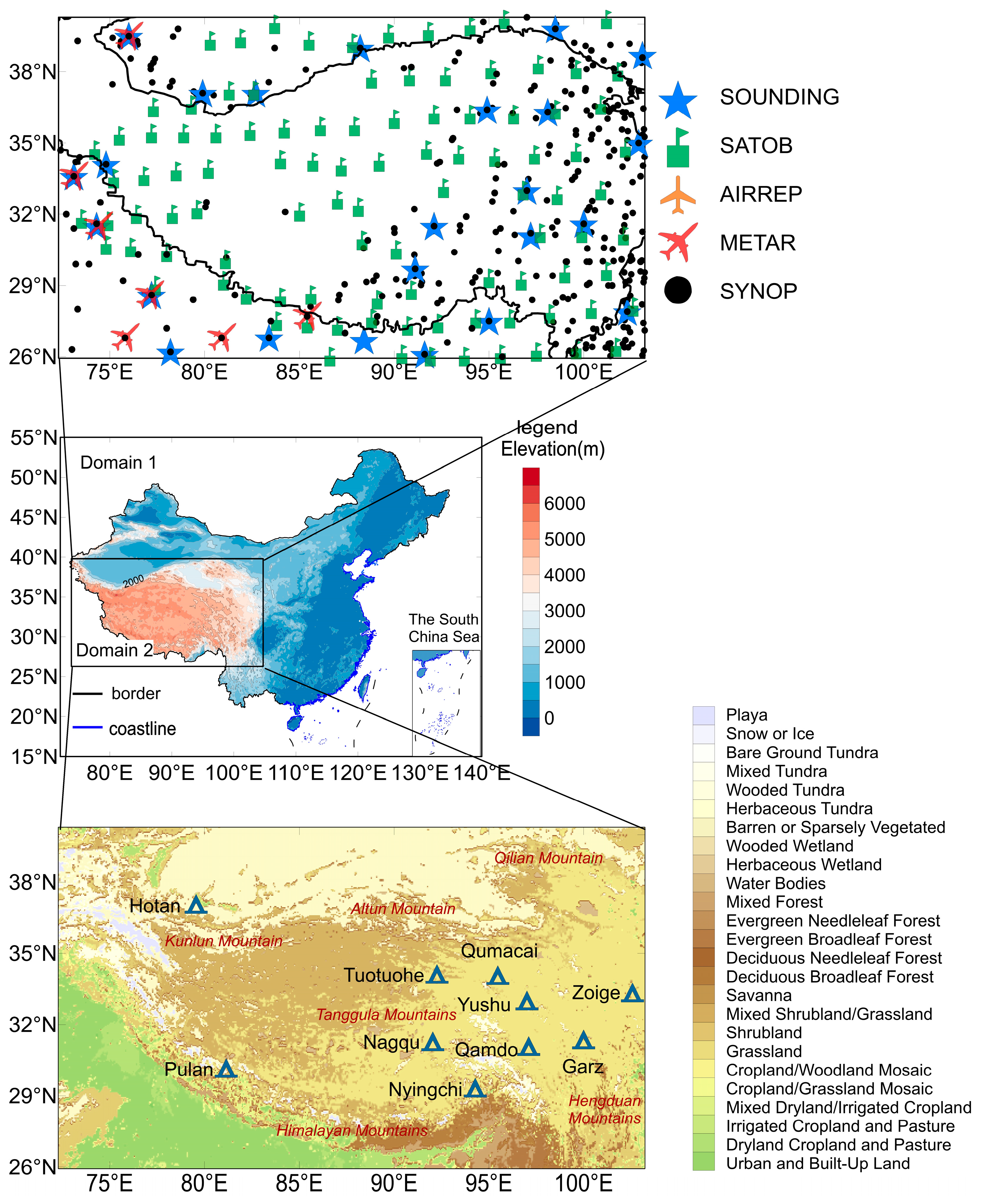
The WRF configuration is presented in Table 1. In this study, a double-nested grid system was utilized, with a horizontal grid spacing of 25 km in domain 1 and 5 km in domain 2 (Figure 2). The two domains used the geographic data resolution of the “usgs_lakes + default” option. The central latitude and longitude of domain 2 are 87.76°E and 33.41°N, and the latitude and longitude of domain 2 ranges from 72.3 to 103.2°E and from 25.9 to 40.3°N, respectively. The National Centers for Environmental Prediction (NCEP) Final Analysis with a 6-h resolution and 1 degree × 1 degree spatial resolution were used as the initial and lateral boundary conditions for the WRF model. The data were obtained from the Global Forecast System (GFS). The simulation covered a period of 10 years, starting on 1 January 2010, at 00:00 UTC and ending on 31 December 2020, at 23:00 UTC.

2.2. Introduction to NCEP_ADP Data and Assimilation Methods

For the assimilation data source, global observation data from the National Centers for Environmental Prediction (NCEP) Automated Data Processing (ADP) was utilized. The timeframe of this data spans from 1 January 2010 to 31 December 2020, and was incorporated into the WRF-3DVAR system for assimilation.
The NCEP-ADP data contain surface synoptic observations (SYNOP), radio-sounding data (SOUNDING), satellite observations (SATOBs), and a few aircraft reports (AIRREPs) and the Meteorological Terminal Air Report (METAR). Satellite observations (SATOBs) track cloud and wind data using cloud motion obtained using space-borne infrared derivations or water vapor imagers. These data and reports include air pressure, geopotential height, air temperature, dew point temperature, wind direction, and wind speed, with up to 20 layers of upper-air observations available ranging from 1000 to 10 hPa. The reporting intervals range from hourly to 12 h (https://rda.ucar.edu/datasets/ds461.0/, accessed on 31 December 2020).
The NCEP-ADP was used in the NCEP-FNL analysis. However, due to the resolution of FNL data being 1 × 1 degree, it is difficult to reconcile multiple observation data within a grid when assimilating these dense observation data. Therefore, when using the WRF model with 3DVAR method for assimilation, we not only increase the grid resolution, but also consider some control and constraint options when setting assimilation parameters to better iterate and converge. For example:
(1)
The multi-level q adjustment should be made while ensuring the conservation of column-integrated water vapor, considering the need to verify the supersaturation (RH > 95%) and the minimum relative humidity (RH < 11%) requirements.
(2)
The assimilation of surface observations will rely on the surface similarity theory within the planetary boundary layer instead of using the lowest model level’s first guess.
(3)
Any stations where the model’s interpolated height differs from the actual observation station’s height by more than 100 m will be deemed invalid and excluded.
(4)
This specifies the method used to interpolate the background into the observation space. The method involves selecting the neighboring model grid point with the smallest height difference, while disregarding the grid points over water.
Figure 2 shows a schematic diagram of the simulated region, underlying land use/vegetation types, and distribution of the NCEP_ADP observation data. It can be seen that the surface SYNOP and SOUNDING sites are mostly distributed in the eastern part of the QTP, whereas there are only a few ground and radio-sounding sites in the western part of the plateau. SATOBs were evenly distributed in the entire simulated region. A few AIRREPs and the METAR are available for the areas south of the Himalayas.
The three-dimensional variational assimilation theory entails the minimization of the cost function as follows [61,62]:
J = 1 2 H x y 0 T R 1 H x y 0 + x x b T B 1 x x b
where y0 is the observed data, x is the model state, xb is the background guess, and B is the background error covariance matrix. The first term of the cost function represents the difference between the observed data and the model state, and the second term represents the difference between the model state and the background. The purpose of the assimilation process is to minimize the cost function, which means that the difference between the observed data and the model state is reduced as much as possible, and the background error is controlled [63]. The last stage involves updating the lower boundary and inserting the analysis obtained from the WRF data assimilation system into the WRF model. This study utilizes a cycling assimilation approach that incorporates a quasi-isentropic coordinate for the analysis increment. By utilizing the potential temperature structure around the observation, this method dynamically adjusts the impact of observations. The 6 h update cycle guarantees that the analysis and short-term forecast remain current [46].
Every 6 h, the cycling 3DVAR technique assimilates recent observations by utilizing the previous 6 h model output as a reference to generate a fresh estimate of 3D atmospheric fields. The approach involves analyzing the observation-minus-simulation residuals, or innovations, to obtain a 3D multivariate error field estimate known as the analysis increment. This increment is then combined with the 6 h forecast background to produce the updated analysis. Through the model’s filter, the 6 h forecast incorporates insights from previous observations into the current analysis [46]. The 3DVAR system operates in cycling mode, which allows the background cloud water and rainwater from the previous cycle to be incorporated into the current cycle. By including these variables in the 3DVAR system, their information can be transferred to the subsequent cycle, reducing the time required for the model’s cloud water and rainwater spin-up during the integration from the analysis stage [64]. At the same time, the “SST update” option is turned on to update the lower boundary conditions in the WRF model, including sea surface temperature (SST), background albedo (ALBBCK), green vegetation fraction (GVF), and underlying soil temperature (TMN) once every 6 h. These variables are updated to the forecast file via “warm start” after the assimilation.
A schematic diagram of the cycling assimilation process is shown in Figure 3.

2.3. Introduction to Observational Data and ERA-5 Data

The National Meteorological Information Center (NMIC) of the China Meteorological Administration (CMA) published the China surface climatic daily dataset (V3.0) on http://data.cma.cn/, accessed on 29 March 2023. This dataset comprises daily meteorological observations from 91 stations located in the simulated QTP region. This dataset includes the daily averaged surface pressure (hPa), 2 m temperature (°C), 2 m relative humidity (%), precipitation (mm), evaporation (mm), 10 m wind direction (°), wind speed (m/s), and ground surface temperature (°C) from 1 January 2010 to 31 December 2019. Before being utilized, the NMIC conducts quality control and inspection on the data. We used these observation data for the model evaluation.
The European Center for Medium-Range Weather Forecasts Reanalysis V5 (ERA-5) reanalysis data were used to provide additional information on atmospheric variables such as temperature, humidity, wind speed, wind direction, and precipitation in the QTP region [65,66]. These data were used in conjunction with the China surface climatic daily dataset to evaluate the performance of the WRF model simulations. To encompass the timeframe from January 2010 to December 2020, monthly mean data from ERA-5 were employed in this investigation. These data cover a 30 km grid and span 137 atmospheric levels, up to 80 km in altitude from the surface [67].
The QTP-HRAD from the WRF model was averaged to a daily time scale for comparison and error analysis with observations from meteorological stations. We also compared the QTP-HRAD with the gridded dataset of ERA-5, comparing variables such as temperature, 2 m temperature, surface temperature, surface pressure, 2 m specific humidity, 10 m wind speed, and total precipitation. We used patch interpolation and the Earth System Modeling Framework (ESMF) re-gridding toolbox in the National Center for Atmospheric Research (NCAR) Command Language (NCL) (https://www.ncl.ucar.edu/Document/Functions/ESMF/ESMF_regrid.shtml, accessed on 8 June 2022) and calculated the difference between the two datasets.

3. Results

3.1. Comparison of Observations and QTP-HRAD Simulations from 10 Weather Stations

We selected 10 stations (Qamdo, Garz, Hotan, Nyingchi, Nagqu, Pulan, Qumacai, Zoige, Tuotuohe, and Yushu) at different locations in and around the QTP as representative stations to compare the daily mean values of the 2 m temperature, relative humidity, precipitation, and evaporation.
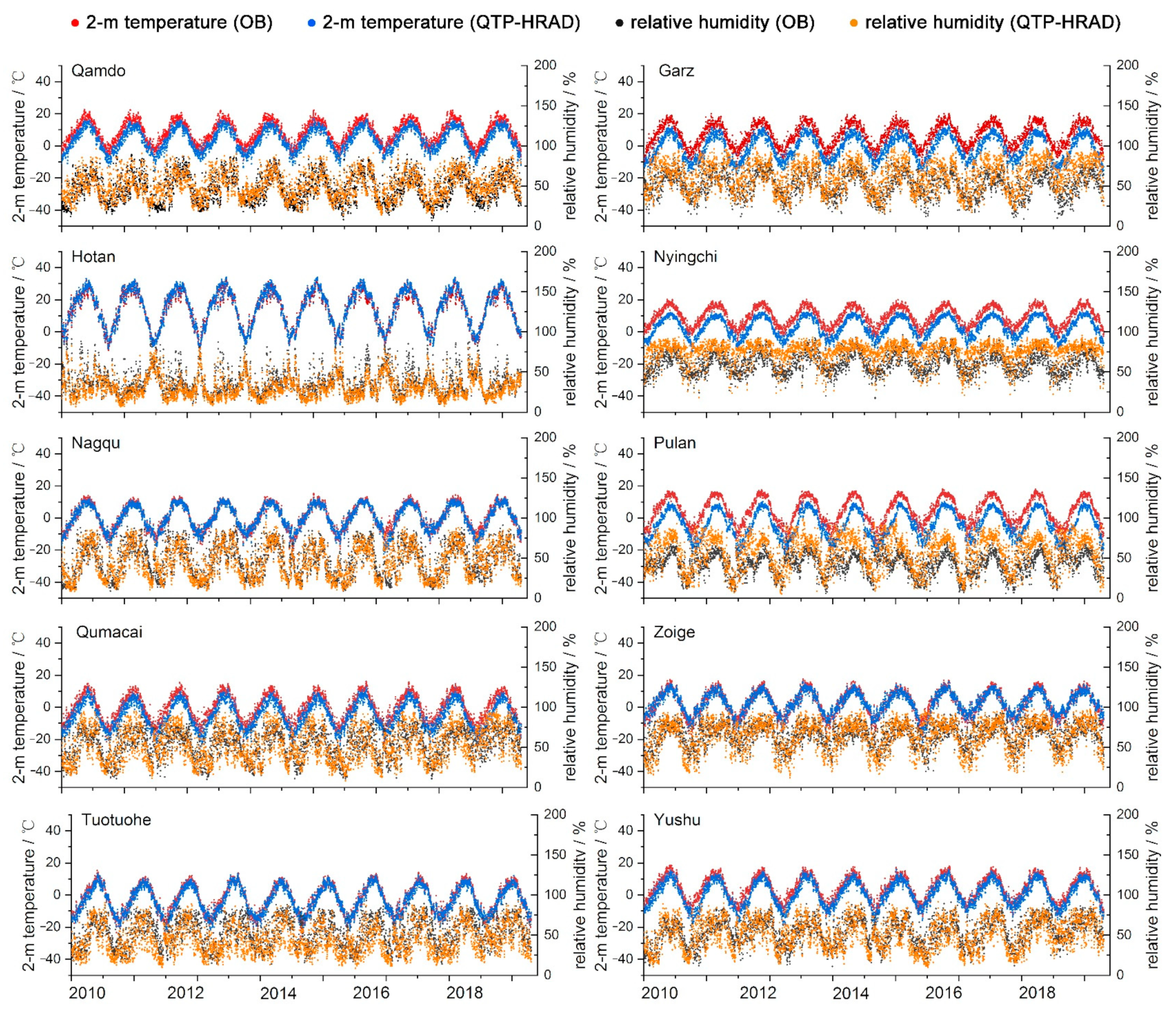
Figure 4 shows the time series comparison of the 2 m temperature and relative humidity observations and the QTP-HRAD data at 10 stations from 2010 to 2019. It can be seen that the observed values of the 2 m temperature at the Garz, Nyingchi, and Pulan stations are all higher than the simulated values throughout the year, and the observed values at the other stations are in good agreement with the QTP-HRAD values. It can also be seen from the error analysis table (Table 2) that the RMSE between the observed and simulated daily mean 2 m temperatures of the Garz, Nyingchi, and Pulan stations are higher than 6.8 °C, and the bias is below −6.6 °C. The RMSE and bias of the other stations between the observations and simulations were lower in the Hotan, Nagqu, Zoige, and Tuotuohe stations, at approximately 2 °C (RMSE)and between −1 and 1 °C (bias), respectively. The correlation coefficients of the 2 m temperature between the observed and simulated values were all from 0.95 to 0.99 at these 10 stations, which all passed the 95% significance test.
The simulated value of the relative humidity also varied annually. Except for the Hotan station, the simulated values of the other stations showed that the relative humidity peaks in the summer and valleys in the winter, mainly due to the higher temperature in the summer and more water vapor evaporating into the air. The Hotan station is located at the edge of the Taklimakan Desert. Owing to the lack of adequate water supply on the underlying surface, less water vapor evaporates into the atmosphere in the summer. The relative humidity increases in the winter when the temperatures are lower, and therefore, the annual variation in the relative humidity and temperature is reversed. Both the observed and simulated results reflect this trend. The average annual relative humidity and specific humidity at the Hotan station are 37% and 4.1 g/kg, respectively, which are much lower than those at the other stations. The statistical error results (Table 2) show that the RMSE and bias of the specific humidity in the Hotan station are the lowest among the 10 observation stations (0.75 and 0.26 g/kg, respectively). The Garz station, located in southeast Tibet, has the highest annual average relative humidity of 79% and a specific humidity of 5.1 g/kg.
In general, the WRF model showed a good simulation effect on the 2 m temperature and relative humidity in the QTP region. The daily averaged simulated values were consistent with the observed values, and accurately reflected the annual and interannual variations in the temperature and humidity. For some stations located in the complex terrain area, the simulation errors for the temperature and humidity were slightly larger than those in the flat terrain area. As the Garz and Nyingchi stations are located in the Hengduan Mountains in the southeast of the QTP, and the Pulan station is located in the Ali Plateau in the southwest of the QTP, the complex and steep terrain caused a large 2 m temperature simulation error. Other stations such as Hotan are located in the Tarim Basin north of the Kunlun Mountains on the northern side of the QTP. The Zoige station is located in the flat Zoige Wetland in the east of the QTP, and the Nagqu station is positioned in the northern QTP on hilly terrain that lies between the Tanggula Mountains, Nyainqentanglha Mountains, and Gangdise Mountains. The terrain of the area gently slopes.
Figure 5 shows a comparison of the daily total precipitation and the daily mean actual evaporation at 10 stations in the QTP region. The red and blue column lines represent the observed and simulated daily total precipitation, respectively, and the gray line represents the actual simulated daily evaporation. As no actual evaporation was observed, only the simulated evaporation was plotted on the graph. It can be seen that the annual variations of the simulated and observed precipitation were relatively consistent, with more precipitation in the summer and less in the winter. Except for the Hotan station, the maximum daily precipitation of the other stations can reach between 30 and 40 mm in the summer, or even 50 mm, which indicates heavy rain and rainstorm. The simulated value reflects the peak value of summer precipitation. At the Pulan station, more precipitation days were observed than those that were simulated. At the Nyingchi station, the observed precipitation in the winter was slightly greater than the simulated value. The annual evaporation was positively correlated with the precipitation. The daily average value of evaporation in the summer is approximately 2–4 mm/d, and the evaporation in the winter tends to be zero. In general, the stations in the eastern and southern parts of the QTP, such as the Qamdo, Garz, Nyingchi, and Zoige stations, have more precipitation and evaporation, while the western stations and the stations in the arid region on the north side of the plateau, such as Hotan and Tuotuohe, have less precipitation and evaporation. The variation trend of precipitation was simulated well by the WRF model, which was in good agreement with the observed values.
The observed and simulated hourly values of 2 m air temperature, dew point temperature, and precipitation at 10 representative stations on the plateau were also compared (figure omitted). The hourly simulated values of some stations are closer to the observed values, such as in the Hotan, Nagqu, Zoige, Tuotuohe, and Yushu stations, but the simulated values of some stations are higher than the observed values by about 3 to 5 °C, such as the Garz, Nyingchi, and Pulan stations. The simulated hourly precipitation can also reflect sporadic precipitation events over the plateau in the summer. At the Hotan and Pulan stations, precipitation events rarely occur, and the simulated value is almost zero. The large bias between the hourly simulation values and the observation values at stations such as Garz, Nyingchi, and Pulan is caused by the large difference between the model grid altitude and the station altitude under complex terrain. Therefore, it is recommended to make corrections to the “pressure-altitude” height difference in order to make better comparisons between the assimilation data and the station observation data.
It can be seen from Table 2 that the RMSE between the observed and simulated 2 m temperatures at the Garz, Pulan, and Nyingchi stations are higher at 8.39, 8.66, and 6.84 °C, respectively, and the bias is negative, indicating that the simulated values are lower than the observed values. Nevertheless, the correlation coefficient was above 0.95 at these 10 stations and passed the 95% confidence test, indicating that the daily variations in the simulated and observed values are in good agreement. The RMSE between the observed and simulated values of the specific humidity at the 10 stations was all below 1.24 g/kg, and the bias was also negative. The minimum bias value appeared in Zoige (−0.22 g/kg). The error statistics of the surface pressure show that the observed and simulated values of the RMSE and bias in the Nagqu, Hotan, and Zoige stations are lower than those at the other stations, which are approximately 10 hPa, and the RMSE and bias between the simulated and observed values of the 2 m temperature and specific humidity were also lower in these three stations. The RMSE between the simulated and observed surface pressure in the Garz, Pulan, and Nyingchi stations were higher, which was above 60 hPa, and the simulated 2 m temperature and specific humidity also showed a larger bias compared with the observations. This may be due to the large difference in altitude between the observation site and the grid corresponding to the model, which increases the simulation errors of other meteorological elements, such as temperature and humidity. The simulated value can be corrected using the actual altitude of the observation site to reduce the errors. From the simulation error results of the 10 m wind speed, the correlation coefficient of only two sites failed the 95% confidence test, and the RMSE and bias of the simulated and observed values of the 10 sites were between 1 and 2 m/s. For high altitude complex terrain mountain areas, the location and orientation of the weather stations, as well as the type of underlying surface, can significantly impact the simulation accuracy of the temperature, humidity, wind direction, and wind speed. Table 2 shows that the root mean square error (RMSE) and bias of the temperature, humidity, and wind speed are also significant when there is a large difference between the simulated and observed atmospheric pressure values at the stations. For instance, the bias of the observed and simulated surface pressure values at the Garz, Nyingchi, and Pulan stations reaches −93.84, −74.89, and −62.44 hPa, respectively. Meanwhile, the bias of the observed and simulated 2 m temperature values at the three stations also reached −8.11, −6.61, and −8.24 °C, respectively, with the RMSE values of 8.39, 6.84, and 8.66 °C. This may be due to the significant difference in elevation between the simulated grid and the observation site. Despite generating 5×5 km horizontal simulation data in the QTP region, the grid distance of 5 × 5 km is still relatively coarse compared to these sites. At the Hotan, Nagqu, and Zoige stations, there was little difference between the simulated surface pressure and observed values, and the simulated 2 m temperature, relative humidity, and wind speed were also consistent with the observed values. The RMSE and bias of the 2 m temperature and humidity were the lowest among the ten representative stations. This is likely because the three stations are not obstructed by high mountains and the terrain is relatively flat, and the elevation of the observation stations is close to that of the model grid points. When using these simulation data, it is better to correct the altitude to reduce the error.

3.2. Comparison of Observations and QTP-HRAD over QTP Region

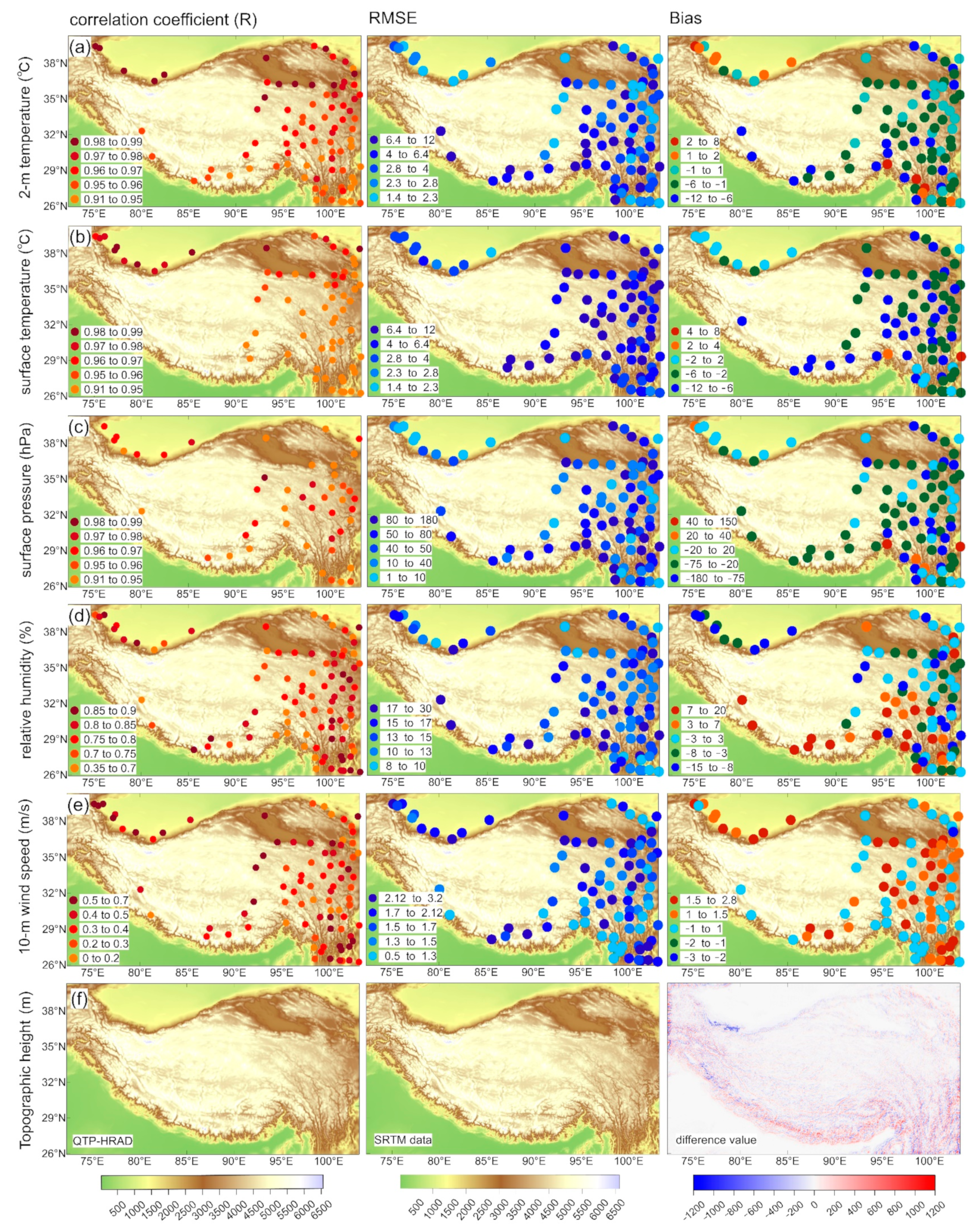
We selected 91 meteorological stations located in the QTP from 2010 to 2019 to compare the statistical errors between the simulated and observed daily mean values of the 2 m temperature, surface temperature, surface pressure, relative humidity, and 10 m wind speed, and plotted the regional distribution of the correlation coefficients, RMSE, and bias. Since most observation stations are located in the eastern part of the plateau, with fewer in the north of the Kunlun Mountain and Altun Mountain, there are almost no meteorological observation stations in the central and western parts of the plateau.
It can be seen from Figure 6a that the correlation coefficients of the 2 m temperature between the observed and simulated values are all above 0.9, and those in the north of the plateau are above 0.97. The RMSE ranged from 1.4 to 12 °C. The RMSE of some stations in the eastern and northern parts of the QTP was lower, while the RMSE of stations along the Himalayan Mountains, Tanggula Mountains, and Qilian Mountains was higher. This may be caused by the large difference between the station altitude and the model grid altitude owing to the complex topography of the mountains. A total of 70% of the stations (64 stations) had negative bias values, indicating that the simulated values were lower than the observed values, and only some stations in the southeastern plateau and north of the Kunlun Mountains had a positive bias. The statistical error distribution of the land surface temperature was similar to the 2 m temperature (Figure 6b), and the correlation coefficient between the simulations and the observations was slightly lower than that of the 2 m temperature. However, the correlation coefficient for almost all stations exceeded 0.9. The RMSE and bias of the surface temperature were larger than those of the 2 m temperature. The RMSE of 70% of the stations (64 stations) was above 4 °C, and the bias of 85% of the stations (76 stations) was negative. This may be due to the underestimation of the air and surface temperatures in the QTP by the NCEP data of the forcing field in the WRF model. Studies have shown that the temperature in the QTP is underestimated in the NCEP data [68,69]. According to the research conducted by Frauenfeld et al. [70], there was an approximate difference of 7 °C between the ERA-40 reanalysis data and the observations. Similarly, Baolin et al. [71] discovered that the NCEP reanalysis data significantly underestimated the observational data for the QTP.
As shown in Figure 6c, the correlation coefficient between the observed and simulated values of the surface pressure was above 0.9. There were 17 stations with the RMSE exceeding 80 hPa, accounting for 19% of all stations, and only 15 stations had an RMSE between 1 and 10 hPa, accounting for 16.7% of the total. The distribution of bias also showed that the values of the simulated surface pressure at 68 stations were lower than the observed values, and 50% of the stations had a bias between −20 and −75 hPa. The low simulated surface temperature values can be explained by the simulation error of the surface pressure. The average elevation of the model grid cell was higher than the elevation of the observation station point, which led to a low simulated surface pressure and low simulated 2 m and surface temperatures.
The correlation coefficients between the observed and simulated values of relative humidity between 0.35 and 0.9, all passing the 95% significance level test, are illustrated in Figure 6d. The RMSE with 60 stations (66.7%) was less than 15%, and only 14 stations had an RMSE between 17% and 30%. The bias of stations along the Himalayan Mountains and near the Hengduan Mountains was positive (30 stations, accounting for 33%), indicating that the simulated value was higher than the observed value. The simulation error of the 10 m wind speed showed that the simulated value of the wind speed at most stations was approximately 2 m/s higher, and 21 stations had a correlation coefficient higher than 0.5, accounting for 24% of the total (Figure 6e). The RMSE ranged between 0.5 and 3.2 m/s, and the bias error statistics showed that the bias in most of the stations was positive (60 sites), and the simulated value was higher than the observed value. The simulated wind speed in the WRF model was high, possibly because the model underestimated the roughness of the underlying surface. This is because the simulation of the wind speed requires the consideration of many parameterization schemes, such as turbulence parameterization schemes and boundary layer parameterization schemes, and the inaccurate estimation of parameters, such as surface roughness, within these schemes can cause errors. Due to the uncertainty and randomness of atmospheric turbulence, the current mesoscale meteorological models have a lower simulation accuracy for the wind speed compared to other variables such as temperature, humidity, and atmospheric pressure [72]. Due to the complex terrain and the limited data input into the meteorological model, the deviation of the average wind speed between the simulation and observation can reach 2 m/s, and the RMSE can be as high as 6 m/s. Even with better models, reducing uncertainties in the simulations of near-surface wind speed and direction can be challenging, as they stem from random or turbulent fluctuations. Furthermore, the randomness is compounded by variations in sub-grid topography and land use [72,73,74].
Overall, the QTP-HRAD showed good results for the QTP. Except for the wind speed, the correlation coefficients between the simulated and observed values of the temperature, humidity, and surface pressure were higher than 0.8. However, the QTP-HRAD underestimated the air temperature and surface temperature in the QTP region, and underestimated the surface pressure at most observation stations, with simulated biases ranging from −20 to −180 hPa. The model overestimated the relative humidity at the southern and southeastern stations and underestimated the relative humidity in the northern part of the plateau. The simulated wind speed value of the QTP-HRAD was higher, and the bias was between 1 and 2.8 m/s.

3.3. Comparison of QTP-HRAD and ERA-5 Data over QTP Region

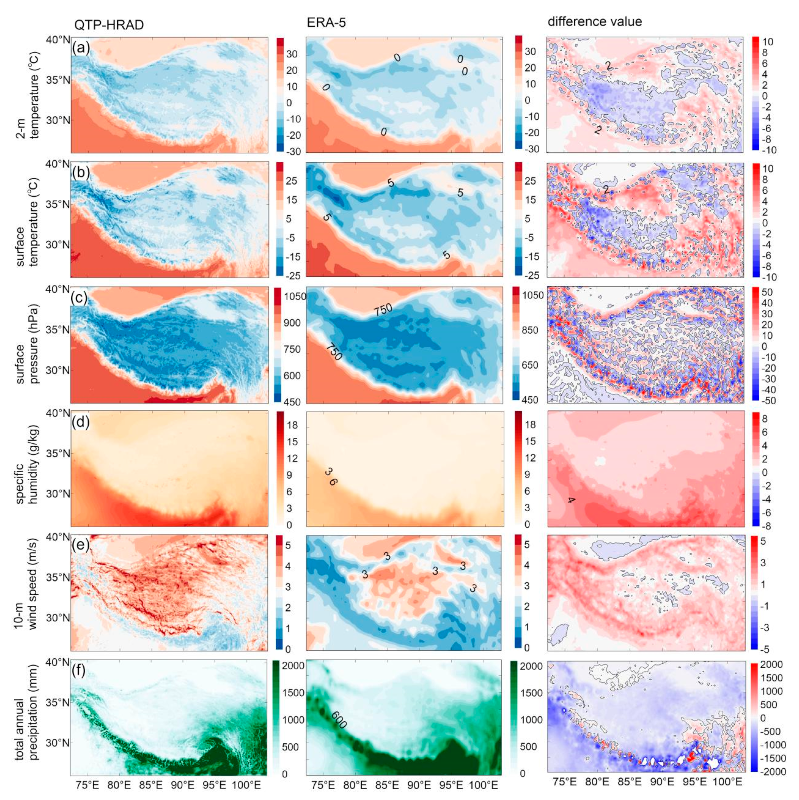
We compared the QTP-HRAD data with the ERA-5 data for 2020 and calculated the difference between the QTP-HRAD and ERA-5 data in the QTP. To calculate the difference, we used bilinear interpolation to scale up the QTP-HRAD data from 5 × 5 km to 0.25° × 0.25°, corresponding to the grid size of the ERA-5 data, and then subtracted. Six meteorological elements, including 2 m temperature, land surface temperature, surface pressure, 2 m specific humidity, 10 m wind speed, and annual accumulated precipitation were compared.
Figure 7 shows the spatial distribution of the QTP-HRAD and ERA-5. As can be seen from Figure 7, the spatial distribution characteristics of the meteorological elements of the QTP-HRAD are consistent with those of the ERA-5, which reflects the distribution of the 2 m temperature, surface pressure, specific humidity, and 10 m wind speed over the QTP. As the spatial resolution of the QTP-HRAD is 5 × 5 km, the distribution of near-surface meteorological elements is finer than that of the ERA-5, which can better demonstrate the differences caused by large topographic fluctuations.
The spatial distribution of the 2 m temperature data is depicted in Figure 7a. In the plateau, the annual average temperature at this height is below 0 °C, with the western part of the plateau having a temperature of around −10 °C, and the eastern part having a temperature of around 0 °C. The 2 m temperature of the ERA-5 is more consistent with the spatial distribution of the QTP-HRAD, but is not as fine as that of the QTP-HRAD. The difference diagram reveals that, with the exception of the central and western regions of the plateau, the difference value is around −4 °C and negative, while the rest of the regions show positive values. The spatial distribution of the surface temperature is comparable to that of the 2 m air temperature. Both the QTP-HRAD and ERA-5 are capable of capturing the extremely low surface temperatures in the western part of the plateau, near the Karakoram Mountains, which are around −15 °C. As the average altitude of the Karakoram Mountains is above 5500 m, the annual 0 °C isotherm is approximately the same as the 4200 m contour line, which is caused by low temperatures throughout the year in the vast mountainous area. From the difference map of the surface temperature, it can be seen that the difference between the central and western parts of the plateau and the Qaidam Basin in Qinghai Province was also found to be negative, and the lowest value was under −5 °C. This value was positive in the central and northern parts of the plateau and the southeastern Hengduan Mountains (6–10 °C).
The regional distribution of the annual average surface pressure is as follows: the surface pressure in the plateau area is low (below 600 hPa), where the lowest in the central and western parts of the plateau can reach 500 hPa, and the surface pressure in the Qaidam Basin on the north side of the plateau is approximately 700 hPa. The areas with significant discrepancies between the QTP-HRAD and ERA-5 are primarily located along the southern Himalayas and the northern Kunlun Mountains, Altun Mountains, and Qilian Mountains. The difference in surface pressure is between −50 and 50 hPa (Figure 7c). The 2 m specific humidity of the QTP-HRAD is a high value area in the south of the Himalayan Mountains, above 10 g/kg, while the annual average specific humidity in the plateau area is approximately 5 g/kg. The specific humidity of the ERA-5 is lower than that of the QTP-HRAD in the plateau area at approximately 3 g/kg, and the difference value is positive (Figure 7d). The 10 m wind speed of the QTP-HRAD in the eastern part of the plateau is below 3 m/s, and the wind speed in other parts of the plateau is higher. The ERA-5 data only reflect that the wind speed in the central and western regions of the plateau is higher than 3 m/s, whereas the wind speed in the Pamir Plateau and Hengduan Mountains is lower than 1 m/s (Figure 7e). As there are only a few surface observation stations in the central and western parts of the plateau, the QTP-HRAD and ERA-5 data have large differences in the 10 m wind speed simulation of the Pamir region, and more observational data need to be obtained in the future for verification. The spatial distribution of the total annual precipitation is shown in Figure 7f. Along the Himalayan Mountains, the precipitation on the southern side can reach more than 2000 mm/year, which occurs on the windward slope and Hengduan Mountains in the southern QTP, while the precipitation in the hinterland of the plateau is less than 200 mm/year. There is slightly more precipitation in the eastern part of the plateau, which is between 500 and 1000 mm/year, and the difference between these two datasets is positive in the southeastern part of the plateau, and negative in other areas, indicating that the total annual precipitation simulated by the QTP-HRAD is higher than that of the ERA-5 (Figure 7f).

4. Data Records and Availability

The assimilation data in the QTP were generated with a spatial resolution of 5 × 5 km at a temporal resolution of once every hour from 2010 to 2020. The assimilation data include 28 near-surface meteorological variables, including the radiation and energy field variables. The latitude and longitude of the dataset area range from 72.3°E to 103.2°E and from 25.9°N to 40.3°N. This dataset began at 00:00 (UTC) on 1 January 2010 and ended at 23:00 (UTC) on 31 December 2020, which includes the 2 m temperature (K), land surface temperature (K), relative humidity (%), surface pressure (Pa), 2 m water vapor mixing ratio (kg/kg), 10 m U and V wind components (m/s), 10 m wind speed (m/s), wind direction (°), precipitation (mm), and dew point temperature (°C), are available online (https://doi.org/10.57760/sciencedb.01840, accessed on 31 December 2020).
The structure of the dataset is as follows:
<Year-Short_name>.nc. Here, “Year” represents the data of a certain year, and “Short_name” represents the short name of the variable as presented in Table 3. The “Short_Name”, “Long_name”, “Missing_value”, and the “Unit” of the variables are also summarized in Table 3. From 2010 to 2020, there are 8760 times per variable in each year, and 8784 times in leap years (2012, 2016, and 2020), and the variables are double-precision floating-point data (float type).

5. Conclusions

The WRF model and its assimilation system can precisely replicate the near-surface meteorological parameters in the QTP region, and the simulation data time series demonstrated good correspondence with the observed data. The simulation results reflect the interannual variations and regional distribution characteristics of meteorological field elements such as temperature, humidity, precipitation, evaporation, air pressure, and wind speed. A comparison between the observations and simulations shows that the simulated values are more consistent with the observations in flat areas, whereas the statistical error is larger in areas with complex terrain conditions. The main conclusions of this study are as follows:
  • We selected 10 representative weather stations in the QTP region and compared the observed and simulated values of the 2 m temperature, relative humidity, and precipitation for the period 2011–2020. It was found that the simulated surface pressure bias and RMSEs of the stations located in complex mountainous and terrain areas on the plateau were significantly different from the observed values. The bias between the observed and simulated surface pressure values at the Garz, Nyingchi, and Pulan stations were −93.84 hPa, −74.89 hPa, and −62.44 hPa, respectively, and the temperature and relative humidity bias of these sites were also large. However, at the stations with relatively flat terrain on the plateau such as Hotan, Nagqu, and Zoige, the disparities between the simulated and observed surface pressure values were minor, and the simulated values of the 2 m temperature, relative humidity, and wind speed were mostly in agreement with the observed values.
  • The annual variations in the simulated and observed precipitation are relatively consistent. The simulated values can reflect the peak periods and magnitudes of summer precipitation on the plateau. The daily average evaporation and precipitation at the 10 stations show a significant positive correlation. The daily average evaporation in the summer is about 2–4 mm/d, while in the winter, it tends to be zero. Overall, there is more precipitation and evaporation at the stations in the eastern and southern parts of the QTP, such as Qamdo, Garz, Nyingchi, and Zoige, while the stations in the western and northern arid areas of the plateau, such as Hotan and Tuotuohe, have less precipitation and evaporation.
  • An error statistical analysis was conducted on the observed and simulated values of the 2 m temperature, surface temperature, surface pressure, relative humidity, and 10 m wind speed at all 91 meteorological stations in the QTP region. It was found that the correlation coefficients of the 2 m temperature, surface temperature, and surface pressure were relatively high, all above 0.9. The correlation coefficient between the observed and simulated values of relative humidity was around 0.7 for most stations on the plateau, with positive bias at the stations in the southern part of the plateau and negative bias at the stations in the northern part. The correlation coefficient between the observed and simulated values of wind speed was relatively low, around 0.5, with positive bias at most stations on the plateau, indicating that the simulated values of the near-surface wind speed were higher than the observed values.
  • We also compared the QTP-HRAD with ERA-5 on a regional scale and calculated their differences. The spatial distribution patterns of the two datasets for the 2 m temperature and surface temperature are quite consistent, with the QTP-HRAD values slightly lower than the ERA-5 in the southwest region of the plateau. The difference in the surface pressure between the two datasets shows clear positive and negative differences along the plateau boundary. The QTP-HRAD simulated specific humidity is about 2–5 g/kg higher than the ERA-5. The simulated values of the 10 m wind speed near the ground are also higher than the ERA-5, except for the central plateau area, with a difference of 1–3 m/s. The simulated precipitation amount shows the largest difference along the southern side of the plateau, particularly along the Himalayan range, and the annual total simulated precipitation amount by the QTP-HRAD is higher than that of the ERA-5.
When using the QTP-HRAD, it should be noted that the grid data near the Himalayan Mountains in the south, the Hengduan Mountains in the southeast, and the Kunlun Mountains in the northwest of the plateau may be inaccurate, which is the limitation of using this dataset.

Author Contributions

Conceptualization, X.W. and S.L.; methodology, M.L.; software, S.Z.; validation, X.Y. and Z.Z.; formal analysis, M.C.; investigation, Y.Z.; writing—original draft preparation, X.W.; writing—review and editing, X.Z. and Y.Q. All authors have read and agreed to the published version of the manuscript.

Funding

The Second Tibetan Plateau Scientific Expedition and Research Program (STEP) (grant number 2019QZKK010304), the National Natural Science Foundation of China (grant number 41975096 and 41975130), the Innovation Team Fund of Southwest Regional Meteorological Center, the China Meteorological Administration (unnumbered), the Science and Technology Program of Sichuan Province (grant number 2022YFS0536), The Open Grants of the State Key Laboratory of Severe Weather (2023LASW-B08) and the Technological Innovation Capacity Enhancement Program of the Chengdu University of Information Technology (grant number KYQN202203) provided financial support for this study.

Data Availability Statement

The hourly values of 2 m temperature, land surface temperature, relative humidity, surface pressure, water vapor mixing ratio, 10 m U and V wind components, precipitation, and dew point temperature at 5 × 5 km are available online at https://doi.org/10.57760/sciencedb.01840 (accessed on 31 December 2020). Due to the extensive amount of work required to validate and compare the dataset with other reanalyzed datasets, this will be our main focus for future research. After publishing this dataset online, we welcome researchers to validate and compare the dataset, and provide us with feedback for further improvement. If there are any questions during the use of the dataset, please contact [email protected].

Acknowledgments

We express our gratitude to the computing resources and assistance provided by the School of Atmospheric Sciences, Chengdu University of Information and Technology (SAS, CUIT).

Conflicts of Interest

The authors declare no conflict of interest.

References

  1. Qiu, J. The third pole: Climate change is coming fast and furious to the Tibetan plateau. Jane Qiu reports on the changes atop the roof of the world. Nature 2008, 454, 393–397. [Google Scholar] [CrossRef] [PubMed]
  2. Immerzeel, W.W.; van Beek, L.P.H.; Bierkens, M.F.P. Climate change will affect the Asian water towers. Science 2010, 328, 1382–1385. [Google Scholar] [CrossRef] [PubMed]
  3. Immerzeel, W.W. Importance and vulnerability of the world’s water towers. Nature 2020, 577, 364–369. [Google Scholar] [CrossRef] [PubMed]
  4. Pepin, N. Elevation-dependent warming in mountain regions of the world. Nat. Clim. Chang. 2015, 5, 424–430. [Google Scholar] [CrossRef]
  5. Liu, X.; Cheng, Z.; Yan, L.; Yin, Z.Y. Elevation dependency of recent and future minimum surface air temperature trends in the Tibetan Plateau and its surroundings. Glob. Planet Change 2009, 68, 164–174. [Google Scholar] [CrossRef]
  6. Yao, T. Tackling on environmental changes in Tibetan Plateau with focus on water, ecosystem and adaptation. Sci. Bull. 2019, 64, 417. [Google Scholar] [CrossRef]
  7. Yao, T. Recent Third Pole’s rapid warming accompanies cryospheric melt and water cycle intensification and interactions between monsoon and environment: Multidisciplinary approach with observations, modeling, and analysis. Bull. Amer. Meteor. Soc. 2019, 100, 423–444. [Google Scholar] [CrossRef]
  8. Chen, F.H. The Tibetan Plateau as the engine for Asian environmental change: The Tibetan Plateau Earth system research into a new era. Sci. Bull. 2021, 66, 1263–1266. [Google Scholar] [CrossRef]
  9. Gao, Y.-X.; Tang, M.-C.; Luo, S.-W.; Shen, Z.-B.; Li, C. Some aspects of recent research on the Qinghai-Xizang Plateau meteorology. Bull. Am. Meteorol. Soc. 1981, 62, 31–35. [Google Scholar] [CrossRef]
  10. Ye, D. Some characteristics of the summer circulation over the Qinghai-Xizang (Tibet) Plateau and its neighborhood. Bull. Am. Meteorol. Soc. 1981, 62, 14–19. [Google Scholar] [CrossRef]
  11. Yanai, M.; Li, C.; Song, Z. Seasonal heating of the Tibetan Plateau and its effects on the evolution of the Asian summer monsoon. J. Meteorol. Soc. Japan. Ser. II 1992, 70, 319–351. [Google Scholar] [CrossRef]
  12. Ye, D.-Z.; Wu, G.-X. The role of the heat source of the Tibetan Plateau in the general circulation. Meteorol. Atmos. Phys. 1998, 67, 181–198. [Google Scholar] [CrossRef]
  13. Tsukamoto, O.; Ishikawa, H.; Tamagawa, I. Analysis of aerodynamic and thermodynamic parameters on the grassy marshland surface of Tibetan Plateau. Prog. Nat. Sci. 2002, 12, 36–40. [Google Scholar]
  14. Ma, Y.; Su, Z.; Koike, T.; Yao, T.; Ishikawa, H.; Ueno, K.i.; Menenti, M. On measuring and remote sensing surface energy partitioning over the Tibetan Plateau––From GAME/Tibet to CAMP/Tibet. Phys. Chem. Earth Parts A/B/C 2003, 28, 63–74. [Google Scholar] [CrossRef]
  15. Ma, Y.; Fan, S.; Ishikawa, H.; Tsukamoto, O.; Yao, T.; Koike, T.; Zuo, H.; Hu, Z.; Su, Z. Diurnal and inter-monthly variation of land surface heat fluxes over the central Tibetan Plateau area. Theor. Appl. Climatol. 2005, 80, 259–273. [Google Scholar] [CrossRef]
  16. Ma, Y.; Zhong, L.; Su, Z.; Ishikawa, H.; Menenti, M.; Koike, T. Determination of regional distributions and seasonal variations of land surface heat fluxes from Landsat-7 Enhanced Thematic Mapper data over the central Tibetan Plateau area. J. Geophys. Res. Atmos. 2006, 111, D10305. [Google Scholar] [CrossRef]
  17. Qie, X.; Wu, X.; Yuan, T.; Bian, J.; Lu, D. Comprehensive pattern of deep convective systems over the Tibetan Plateau–South Asian monsoon region based on TRMM data. J. Clim. 2014, 27, 6612–6626. [Google Scholar] [CrossRef]
  18. Zhao, P.; Li, Y.; Guo, X.; Xu, X.; Liu, Y.; Tang, S.; Xiao, W.; Shi, C.; Ma, Y.; Yu, X. The Tibetan Plateau surface-atmosphere coupling system and its weather and climate effects: The Third Tibetan Plateau Atmospheric Science Experiment. J. Meteorol. Res. 2019, 33, 375–399. [Google Scholar] [CrossRef]
  19. Tao, S.; Luo, S.; Zhang, H. The Qinghai-Xizang Plateau Meteorological Experiment (Qxpmex) May–August 1979. In Proceedings of the International Symposium on the Qinghai-Xizang Plateau and Mountain Meteorology, Beijing, China, 20–24 March 1984; American Meteorological Society: Boston, MA, USA, 1986; pp. 3–13. Available online: https://link.springer.com/chapter/10.1007/978-1-935704-19-5_1 (accessed on 31 December 2020).
  20. Wang, J. Land surface process experiments and interaction study in China: From HEIFE to IMGRASS and GAME-Tibet/TIPEX. Plateau Meteorol. 1999, 18, 280–294. [Google Scholar]
  21. Ma, Y.-M.; Yao, T.-D.; Wang, J.-M. Experimental Study of Energy and Water Cycle in Tibetan Plateau—The Progress Introduction on the Study of GAME/Tibet and CAMP/Tibet. Plateau Meteorol. 2006, 25, 344–351. [Google Scholar]
  22. Zhao, P.; Xu, X.; Chen, F.; Guo, X.; Zheng, X.; Liu, L.; Hong, Y.; Li, Y.; La, Z.; Peng, H. The third atmospheric scientific experiment for understanding the earth–atmosphere coupled system over the Tibetan Plateau and its effects. Bull. Am. Meteorol. Soc. 2018, 99, 757–776. [Google Scholar] [CrossRef]
  23. Wang, H.-J.; Sun, J.-Q.; Chen, H.-P.; Zhu, Y.-L.; Zhang, Y.; Jiang, D.-B.; Lang, X.-M.; Fan, K.; Yu, E.-T.; Yang, S. Extreme climate in China: Facts, simulation and projection. Meteorol. Z. 2012, 21, 279. [Google Scholar] [CrossRef]
  24. Dasari, H.P.; Salgado, R.; Perdigao, J.; Challa, V.S. A regional climate simulation study using WRF-ARW model over Europe and evaluation for extreme temperature weather events. Int. J. Atmos. Sci. 2014, 2014, 704079. [Google Scholar] [CrossRef]
  25. Sun, Q.; Zwiers, F.; Zhang, X.; Li, G. A comparison of intra-annual and long-term trend scaling of extreme precipitation with temperature in a large-ensemble regional climate simulation. J. Clim. 2020, 33, 9233–9245. [Google Scholar] [CrossRef]
  26. Sasai, T.; Kawase, H.; Kanno, Y.; Yamaguchi, J.; Sugimoto, S.; Yamazaki, T.; Sasaki, H.; Fujita, M.; Iwasaki, T. Future projection of extreme heavy snowfall events with a 5-km large ensemble regional climate simulation. J. Geophys. Res. Atmos. 2019, 124, 13975–13990. [Google Scholar] [CrossRef]
  27. Altaratz, O.; Koren, I.; Remer, L.; Hirsch, E. Cloud invigoration by aerosols—Coupling between microphysics and dynamics. Atmos. Res. 2014, 140, 38–60. [Google Scholar] [CrossRef]
  28. Morrison, H.; van Lier-Walqui, M.; Fridlind, A.M.; Grabowski, W.W.; Harrington, J.Y.; Hoose, C.; Korolev, A.; Kumjian, M.R.; Milbrandt, J.A.; Pawlowska, H. Confronting the challenge of modeling cloud and precipitation microphysics. J. Adv. Model. Earth Syst. 2020, 12, e2019MS001689. [Google Scholar] [CrossRef]
  29. Zhuo, H.; Liu, Y.; Jin, J. Improvement of land surface temperature simulation over the Tibetan Plateau and the associated impact on circulation in East Asia. Atmos. Sci. Lett. 2016, 17, 162–168. [Google Scholar] [CrossRef]
  30. Meng, X.; Lyu, S.; Zhang, T.; Zhao, L.; Li, Z.; Han, B.; Li, S.; Ma, D.; Chen, H.; Ao, Y. Simulated cold bias being improved by using MODIS time-varying albedo in the Tibetan Plateau in WRF model. Environ. Res. Lett. 2018, 13, 044028. [Google Scholar] [CrossRef]
  31. Peng, Q.; Meixue, Y.; Donglin, G.; Chu-xiong, C. Simulation of summer air temperature and precipitation over Tibetan Plateau with Regional Climate Model (RegCM3). Plateau Meteor. 2009, 28, 738–744. [Google Scholar]
  32. Zhang, D.; Gao, X.; Bai, H.; Li, D. Simulation of climate over Qinghai-Xizang Plateau utilizing RegCM3. Plateau Meteor. 2005, 24, 714–720. [Google Scholar]
  33. Gao, X.; Shi, Y.; Zhang, D.; Giorgi, F. Climate change in China in the 21st century as simulated by a high resolution regional climate model. Chin. Sci. Bull. 2012, 57, 1188–1195. [Google Scholar] [CrossRef]
  34. Gao, Y.; Xu, J.; Chen, D. Evaluation of WRF mesoscale climate simulations over the Tibetan Plateau during 1979–2011. J. Clim. 2015, 28, 2823–2841. [Google Scholar] [CrossRef]
  35. Yu, E.; Sun, J.; Chen, H.; Xiang, W. Evaluation of a high-resolution historical simulation over China: Climatology and extremes. Clim. Dyn. 2015, 45, 2013–2031. [Google Scholar] [CrossRef]
  36. Gao, Y.; Chen, F.; Jiang, Y. Evaluation of a convection-permitting modeling of precipitation over the Tibetan Plateau and its influences on the simulation of snow-cover fraction. J. Hydrometeorol. 2020, 21, 1531–1548. [Google Scholar] [CrossRef]
  37. You, Q.; Min, J.; Zhang, W.; Pepin, N.; Kang, S. Comparison of multiple datasets with gridded precipitation observations over the Tibetan Plateau. Clim. Dyn. 2015, 45, 791–806. [Google Scholar] [CrossRef]
  38. Zhu, X.; Liu, Y.; Wu, G. An assessment of summer sensible heat flux on the Tibetan Plateau from eight data sets. Sci. China Earth Sci. 2012, 55, 779–786. [Google Scholar] [CrossRef]
  39. Su, Z.; De Rosnay, P.; Wen, J.; Wang, L.; Zeng, Y. Evaluation of ECMWF’s soil moisture analyses using observations on the Tibetan Plateau. J. Geophys. Res. Atmos. 2013, 118, 5304–5318. [Google Scholar] [CrossRef]
  40. Zeng, Y.; Su, Z.; Van der Velde, R.; Wang, L.; Xu, K.; Wang, X.; Wen, J. Blending satellite observed, model simulated, and in situ measured soil moisture over Tibetan Plateau. Remote Sens. 2016, 8, 268. [Google Scholar] [CrossRef]
  41. Grose, M.R.; Narsey, S.; Delage, F.; Dowdy, A.J.; Bador, M.; Boschat, G.; Chung, C.; Kajtar, J.; Rauniyar, S.; Freund, M. Insights from CMIP6 for Australia’s future climate. Earth’s Future 2020, 8, e2019EF001469. [Google Scholar] [CrossRef]
  42. Ban, N.; Schmidli, J.; Schär, C. Evaluation of the convection-resolving regional climate modeling approach in decade-long simulations. J. Geophys. Res. Atmos. 2014, 119, 7889–7907. [Google Scholar] [CrossRef]
  43. Collier, E.; Mölg, T.; Sauter, T. Recent atmospheric variability at Kibo Summit, Kilimanjaro, and its relation to climate mode activity. J. Clim. 2018, 31, 3875–3891. [Google Scholar] [CrossRef]
  44. Ekström, M.; Grose, M.R.; Whetton, P.H. An appraisal of downscaling methods used in climate change research. Wiley Interdiscip. Rev. Clim. Chang. 2015, 6, 301–319. [Google Scholar] [CrossRef]
  45. Smith, T.L.; Benjamin, S.G.; Gutman, S.I.; Sahm, S. Short-range forecast impact from assimilation of GPS-IPW observations into the Rapid Update Cycle. Mon. Weather Rev. 2007, 135, 2914–2930. [Google Scholar] [CrossRef]
  46. Benjamin, S.G.; Dévényi, D.; Weygandt, S.S.; Brundage, K.J.; Brown, J.M.; Grell, G.A.; Kim, D.; Schwartz, B.E.; Smirnova, T.G.; Smith, T.L. An hourly assimilation–forecast cycle: The RUC. Mon. Weather Rev. 2004, 132, 495–518. [Google Scholar] [CrossRef]
  47. James, E.P.; Benjamin, S.G. Observation system experiments with the hourly updating Rapid Refresh model using GSI hybrid ensemble–variational data assimilation. Mon. Weather Rev. 2017, 145, 2897–2918. [Google Scholar] [CrossRef]
  48. Ha, S.-Y.; Snyder, C. Influence of surface observations in mesoscale data assimilation using an ensemble Kalman filter. Mon. Weather Rev. 2014, 142, 1489–1508. [Google Scholar] [CrossRef]
  49. Wen, X.; Zhu, X.; Li, M.; Guo, H.; Zhang, S.; Yang, X.; Zheng, Z.; Yan, D.; Zhang, Y.; Lv, S. QTP-HRAD[DS/OL]. V2. Science Data Bank. 2022. Available online: https://www.scidb.cn/en/detail?dataSetId=f0860df1bd8e4fee842baa70fe6d9b94# (accessed on 29 March 2023).
  50. Thompson, G.; Field, P.R.; Rasmussen, R.M.; Hall, W.D. Explicit forecasts of winter precipitation using an improved bulk microphysics scheme. Part II: Implementation of a new snow parameterization. Mon. Weather Rev. 2008, 136, 5095–5115. [Google Scholar] [CrossRef]
  51. Iacono, M.J.; Delamere, J.S.; Mlawer, E.J.; Shephard, M.W.; Clough, S.A.; Collins, W.D. Radiative forcing by long-lived greenhouse gases: Calculations with the AER radiative transfer models. J. Geophys. Res. Atmos. 2008, 113, D13103. [Google Scholar] [CrossRef]
  52. Bae, S.Y.; Hong, S.-Y.; Lim, K.-S.S. Coupling WRF double-moment 6-class microphysics schemes to RRTMG radiation scheme in weather research forecasting model. Adv. Meteorol. 2016, 2016, 5070154. [Google Scholar] [CrossRef]
  53. Tiedtke, M. A comprehensive mass flux scheme for cumulus parameterization in large-scale models. Mon. Weather Rev. 1989, 117, 1779–1800. [Google Scholar] [CrossRef]
  54. Zhang, C.; Wang, Y.; Hamilton, K. Improved representation of boundary layer clouds over the southeast Pacific in ARW-WRF using a modified Tiedtke cumulus parameterization scheme. Mon. Weather Rev. 2011, 139, 3489–3513. [Google Scholar] [CrossRef]
  55. Ek, M.; Mitchell, K.; Lin, Y.; Rogers, E.; Grunmann, P.; Koren, V.; Gayno, G.; Tarpley, J. Implementation of Noah land surface model advances in the National Centers for Environmental Prediction operational mesoscale Eta model. J. Geophys. Res. Atmos. 2003, 108, GCP12-1. [Google Scholar] [CrossRef]
  56. Janjić, Z.I. The step-mountain eta coordinate model: Further developments of the convection, viscous sublayer, and turbulence closure schemes. Mon. Weather. Rev. 1994, 122, 927–945. [Google Scholar] [CrossRef]
  57. Chen, F.; Janjić, Z.; Mitchell, K. Impact of atmospheric surface-layer parameterizations in the new land-surface scheme of the NCEP mesoscale Eta model. Bound.-Layer Meteorol. 1997, 85, 391–421. [Google Scholar] [CrossRef]
  58. Bassett, R.; Young, P.; Blair, G.; Samreen, F.; Simm, W. A large ensemble approach to quantifying internal model variability within the WRF numerical model. J. Geophys. Res. Atmos. 2020, 125, e2019JD031286. [Google Scholar] [CrossRef]
  59. Zhang, X.; Cornuelle, B.D.; Martin, A.; Weihs, R.R.; Ralph, M. West-WRF Sensitivity to Sea Surface Temperature Boundary Condition in California Precipitation Forecasts of AR Related Events. In Proceedings of the AGU Fall Meeting Abstracts, New Orleans, LA, USA, 11–15 December 2017; pp. A33H–2496. [Google Scholar]
  60. Zeng, X.; Beljaars, A. A prognostic scheme of sea surface skin temperature for modeling and data assimilation. Geophys. Res. Lett. 2005, 32. [Google Scholar] [CrossRef]
  61. Ide, K.; Courtier, P.; Ghil, M.; Lorenc, A.C. Unified notation for data assimilation: Operational, sequential and variational (gtspecial issueltdata assimilation in meteology and oceanography: Theory and practice). J. Meteorol. Soc. Japan. Ser. II 1997, 75, 181–189. [Google Scholar] [CrossRef]
  62. Lorenc, A.C. Analysis methods for numerical weather prediction. Q. J. R. Meteorol. Soc. 1986, 112, 1177–1194. [Google Scholar] [CrossRef]
  63. Barker, D.M.; Huang, W.; Guo, Y.-R.; Bourgeois, A.; Xiao, Q. A three-dimensional variational data assimilation system for MM5: Implementation and initial results. Mon. Weather. Rev. 2004, 132, 897–914. [Google Scholar] [CrossRef]
  64. Routray, A.; Mohanty, U.; Osuri, K.K.; Kiran Prasad, S. Improvement of monsoon depressions forecast with assimilation of Indian DWR data using WRF-3DVAR analysis system. Pure Appl. Geophys. 2013, 170, 2329–2350. [Google Scholar] [CrossRef]
  65. Dragani, R.; Hersbach, H.; Poli, P.; Pebeuy, C.; Hirahara, S.; Simmons, A.; Dee, D. Recent Reanalysis Activities at ECMWF: Results from ERA-20C and Plans for ERA5. AGU Fall Meet. Abstr. 2015, 2015, A11R-02. [Google Scholar]
  66. Urraca, R.; Huld, T.; Gracia-Amillo, A.; Martinez-De-Pison, F.J.; Kaspar, F.; Sanz-Garcia, A. Evaluation of global horizontal irradiance estimates from ERA5 and COSMO-REA6 reanalyses using ground and satellite-based data. Sol. Energy 2018, 164, 339–354. [Google Scholar] [CrossRef]
  67. Hersbach, H.; Bell, B.; Berrisford, P.; Hirahara, S.; Horányi, A.; Muñoz-Sabater, J.; Nicolas, J.; Peubey, C.; Radu, R.; Schepers, D. The ERA5 global reanalysis. Q. J. R. Meteorol. Soc. 2020, 146, 1999–2049. [Google Scholar] [CrossRef]
  68. Bao, X.; Zhang, F. Evaluation of NCEP–CFSR, NCEP–NCAR, ERA-Interim, and ERA-40 reanalysis datasets against independent sounding observations over the Tibetan Plateau. J. Clim. 2013, 26, 206–214. [Google Scholar] [CrossRef]
  69. You, Q.; Kang, S.; Pepin, N.; Flügel, W.-A.; Yan, Y.; Behrawan, H.; Huang, J. Relationship between temperature trend magnitude, elevation and mean temperature in the Tibetan Plateau from homogenized surface stations and reanalysis data. Glob. Planet. Change 2010, 71, 124–133. [Google Scholar] [CrossRef]
  70. Frauenfeld, O.W.; Zhang, T.; Serreze, M.C. Climate change and variability using European Centre for Medium-Range Weather Forecasts reanalysis (ERA-40) temperatures on the Tibetan Plateau. J. Geophys. Res. Atmos. 2005, 110, D02101.1–D02101.9. [Google Scholar] [CrossRef]
  71. Baolin, L.; Yichi, Z.; Chenghu, Z. Remote sensing detection of glacier changes in Tianshan Mountains for the past 40 years. J. Geogr. Sci. 2004, 14, 296–302. [Google Scholar] [CrossRef]
  72. Hanna, S.R.; Yang, R. Evaluations of mesoscale models’ simulations of near-surface winds, temperature gradients, and mixing depths. J. Appl. Meteorol. 2001, 40, 1095–1104. [Google Scholar] [CrossRef]
  73. Horvath, K.; Koracin, D.; Vellore, R.; Jiang, J.; Belu, R. Sub-kilometer dynamical downscaling of near-surface winds in complex terrain using WRF and MM5 mesoscale models. J. Geophys. Res. Atmos. 2012, 117, D11111. [Google Scholar] [CrossRef]
  74. Wen, X.; Lu, S.; Jin, J. Integrating remote sensing data with WRF for improved simulations of oasis effects on local weather processes over an arid region in northwestern China. J. Hydrometeorol. 2012, 13, 573–587. [Google Scholar] [CrossRef]
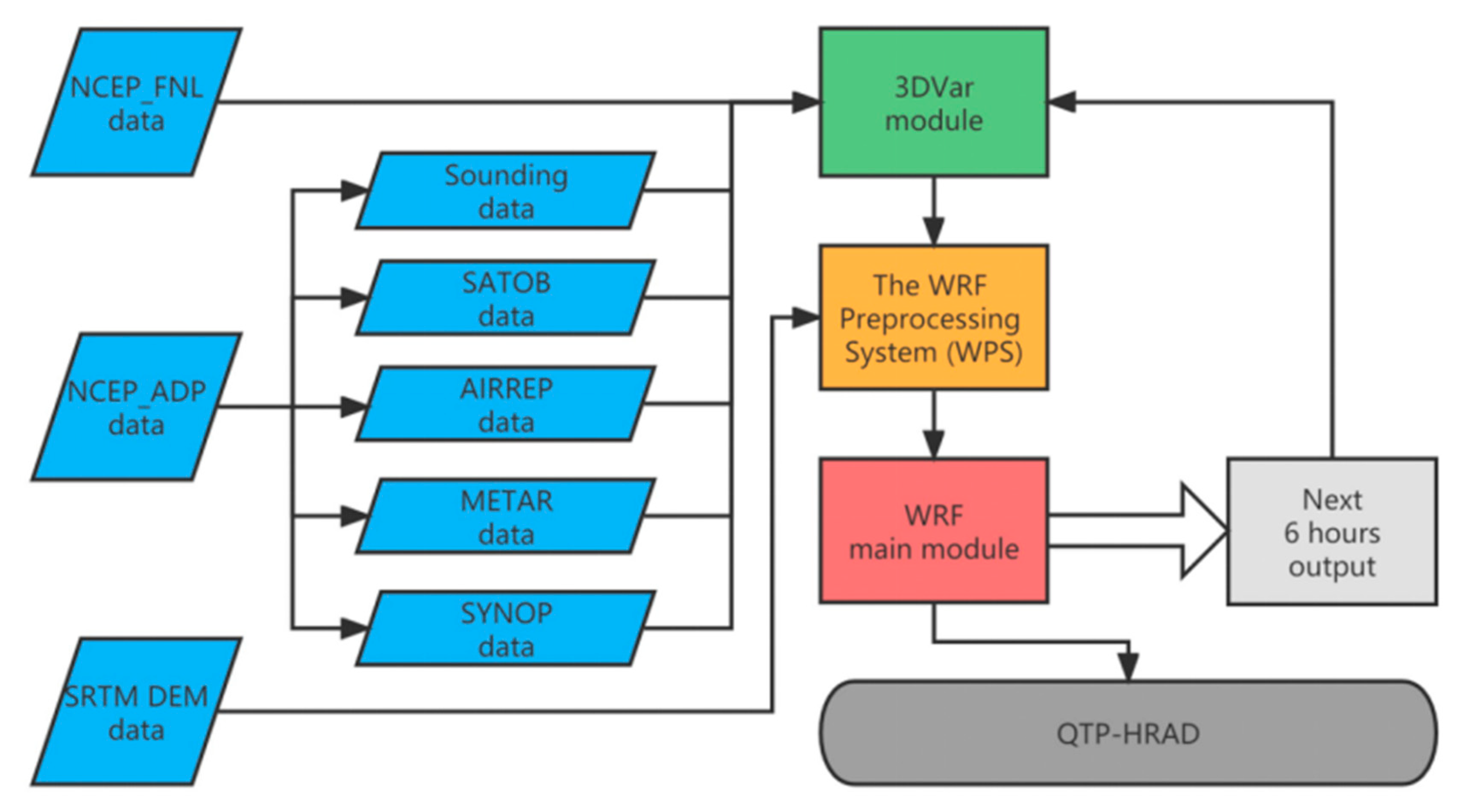
Figure 1. Flowchart for generating the QTP-HRAD.
Remotesensing 15 02906 g001
Figure 2. The schematic diagram of simulated region, underlying land use/vegetation types, and the distribution of the NCEP_ADP observation data. There are a total of 10 stations (Qamdo, Garz, Hotan, Nyingchi, Nagqu, Pulan, Qumacai, Zoige, Tuotuohe, and Yushu) at different locations With the blue triangle in and around the QTP as representative stations. The Hotan station stands on the northwest side of the QTP, located in the northwest arid region, and represents the simulated situation in the arid region north of the plateau. Nyingchi and Qamdo stations are located in the semi-humid and humid regions of the southeastern plateau, representing a simulated situation in the humid region of the southeastern plateau. Except for the Hotan station, which has a lower altitude of 1370 m, all other stations are located in the hinterland of the QTP at an altitude of over 3000 m.
Remotesensing 15 02906 g002
Figure 3. The schematic diagram of cycling assimilation data in the WRF model. The bottom brackets mean every cycle of assimilation, and the bold arrows mean the observations are assimilated from the time window “00”, “06”, “12”, and “18”.
Remotesensing 15 02906 g003
Figure 4. Comparison of observations and QTP-HRAD simulations for daily averaged 2 m temperature (°C) and relative humidity (%) of 10 weather stations in QTP region from 2010 to 2019. The left vertical axis shows the range of 2 m temperature value and the right vertical axis shows the range of relative humidity value.
Remotesensing 15 02906 g004
Figure 5. Comparison of observations and QTP-HRAD simulations for daily precipitation (mm) and evaporation (mm) from 10 weather stations in the QTP region from 2010 to 2019. The left vertical axis shows the range of precipitation values, and the right vertical axis shows the range of evaporation values.
Remotesensing 15 02906 g005
Figure 6. Correlation coefficient, RMSE, and bias between observation and the QTP-HRAD daily mean (a) 2 m temperature (°C), (b) land surface temperature (°C), (c) surface pressure (hPa), (d) relative humidity (%), and (e) 10 m wind speed (m/s) from 2010 to 2019. (f) Topographic height from QTP-HRAD, SRTM data, and the difference value.
Remotesensing 15 02906 g006
Figure 7. Spatial distribution of the QTP-HRAD (left column), ERA-5 (middle column), and their difference values (right column) over QTP region in 2020. The bold black line is the zero contour line. (a) Annual mean 2 m temperature (°C); (b) annual mean land surface temperature (°C); (c) surface pressure (hPa); (d) specific humidity (g/kg); (e) 10 m wind speed (m/s); and (f) total annual precipitation (mm).
Remotesensing 15 02906 g007
Table 1. Summary of the WRF configuration.
Domain ConfigurationDomain 1Domain 2
Horizontal grid spacing25 km5 km
Grid dimensions370 × 270544 × 304
Time step180 s30 s
Central longitude–latitude103°E, 38°N87.76°E, 33.41°N
Geog data resolutionusgs_lakes + defaultusgs_lakes + default
Model physics
MicrophysicsThompson scheme
Cumulus parameterizationTiedtke scheme
Longwave and shortwave radiationRRTMG scheme
Surface layerEta-similarity scheme
Land surfaceNoah land surface model
Planetary boundary layerMellor–Yamada–Janjic scheme
Other physics options for long simulationstmn_update: update deep soil temperature
sst_skin: calculate skin SST based on Zeng and Beljaars [60]
sst_update: update sea-surface temperature, vegetation fraction, albedo
Table 2. RMSE, bias, and correlation coefficient of the daily averaged 2 m temperature, specific humidity, surface pressure, and 10 m wind speed values between observations and QTP-HRAD from 10 weather stations; * means the correlation coefficient passed the significance t-test level of 0.05.
Weather Stations2 m Temperature
(°C)
Specific Humidity
(g/kg)
Surface Pressure
(hPa)
10 m Wind Speed
(m/s)
RMSEBiasRRMSEBiasRRMSEBiasRRMSEBiasR
Qamdo4.88−4.510.96 *1.07−0.510.95 *59.9−59.860.89 *0.221.650.22 *
Garz8.39−8.110.96 *1.14−0.820.96 *93.9−93.840.85 *1.721.290.22 *
Hotan1.350.360.99 *0.75−0.260.96 *11.56−11.450.96 *1.731.340.51 *
Nyingchi6.84−6.610.95 *0.90−0.480.97 *74.93−74.890.79 *1.1510.536−0.15
Nagqu2.01−0.540.97 *0.77−0.390.97 *9.08−9.030.97 *1.541.160.54 *
Pulan8.66−8.240.95 *0.81−0.460.97 *62.48−62.440.85 *1.2590.1170.003
Qumacai4.97−4.430.96 *1.18−0.890.96 *52.21−52.160.95 *2.592.00.23 *
Zoige2.24−0.310.96 *0.73−0.220.97 *8.24−8.1530.96 *1.671.250.33 *
Tuotuohe2.19−1.000.97 *1.24−0.930.95 *20.48−20.460.97 *1.380.440.56 *
Yushu3.68−2.950.96 *1.08−0.780.97 *39.50−39.470.90 *1.671.410.39 *
Table 3. The description and spatiotemporal variables of QTP-HRAD.
Data Description
Data typeGridded
ProjectionMercator projection
Horizontal coverageThe QTP region, 72.3°E to 103.2°E and 25.9°N to 40.3°N
Horizontal resolution0.05° × 0.05°, about 5 × 5 km
Vertical coverageLand surface, 2 m and 10 m above the surface level
Temporal coverageBegan at 00:00 (UTC) 1 January 2010 and ended at 23:00 (UTC) 31 December 2020
Temporal resolutionHourly
File formatNETCDF
Variables of QTP-HRAD
VariablesShort_nameLong_nameMissing_valueUnit
2 m temperaturet2TEMP at 2 m1 × 1030K
Land surface temperaturetskSurface skin temperature1 × 1030K
2 m relative humidityrh2Relative Humidity at 2 m1 × 1030%
Surface pressureprsSfc pressure1 × 1030Pa
2 m water vapor mixing ratioq2QV at 2 m1 × 1030kg·kg−1
10 m U wind componentsu10U at 10 m1 × 1030m·s−1
10 m V wind componentsv10V at 10 m1 × 1030m·s−1
10 m wind speedws10Wind speed at 10 m1 × 1030m·s−1
10 m wind directionwd10Wind direction at 10 m1 × 1030Degrees
PrecipitationpreAccumulated total cumulus precipitation, accumulated total grid scale precipitation1 × 1030
1 × 1030
mm,
mm
2 m dew point temperaturetd2Dewpoint temperature at 2 m1 × 1030°C
Disclaimer/Publisher’s Note: The statements, opinions and data contained in all publications are solely those of the individual author(s) and contributor(s) and not of MDPI and/or the editor(s). MDPI and/or the editor(s) disclaim responsibility for any injury to people or property resulting from any ideas, methods, instructions or products referred to in the content.