Article

Comparison of Machine Learning Methods for Predicting Soil Total Nitrogen Content Using Landsat-8, Sentinel-1, and Sentinel-2 Images

1
College of Mining Engineering, North China University of Science and Technology, Tangshan 063210, China
2
Tangshan Key Laboratory of Resources and Environmental Remote Sensing, Tangshan 063210, China
3
Hebei Industrial Technology Institute of Mine Ecological Remediation, Tangshan 063210, China
4
Collaborative Innovation Center, Green Development and Ecological Restoration of Mineral Resources, Tangshan 063210, China
5
Key Laboratory of Wetland Ecology and Environment, Northeast Institute of Geography and Agroecology, Chinese Academy of Sciences, Changchun 130102, China
6
College of Geography and Ocean Sciences, Yanbian University, Yanji 133000, China
*
Author to whom correspondence should be addressed.
These authors contributed equally to this work.
Remote Sens. 2023, 15(11), 2907; https://doi.org/10.3390/rs15112907
Submission received: 26 April 2023 / Revised: 31 May 2023 / Accepted: 1 June 2023 / Published: 2 June 2023

Abstract

:
Soil total nitrogen (STN) is a crucial component of the ecosystem’s nitrogen pool, and accurate prediction of STN content is essential for understanding global nitrogen cycling processes. This study utilized the measured STN content of 126 sample points and 40 extracted remote sensing variables to predict the STN content and map its spatial distribution in the northeastern coastal region of Hebei Province, China, employing the random forest (RF), gradient boosting machine (GBM), and extreme gradient boosting (XGBoost) methods. The purpose was to compare the ability of remote sensing images (Landsat-8, Sentinel-1, and Sentinel-2) with different machine learning methods for predicting STN content. The research results show the following: (1) The three machine learning methods accurately predicted the STN content and the optimal model provided by the XGBoost method, with an R2 of 0.627, RMSE of 0.127 g·kg−1, and MAE of 0.092 g·kg−1. (2) The combination of optical and synthetic aperture radar (SAR) images improved prediction accuracy, with the R2 improving by 45.5%. (3) The importance of optical images is higher than that of SAR images in the RF, GBM, and XGBoost methods, with optical images accounting for 87%, 76%, and 77% importance, respectively. (4) The spatial distribution of STN content predicted by the three methods is similar. Higher STN contents are distributed in the northern part of the study area, while lower STN contents are distributed in coastal areas. The results of this study can be very useful for inventories of soil nitrogen and provide data support and method references for revealing nitrogen cycling.

1. Introduction

Nitrogen is one of the key essential nutrients for plant growth and development [1]. Low levels of nitrogen can negatively impact plant growth, while excessive nitrogen levels can lead to reduced ecosystem productivity and environmental pollution [2,3]. Soil is a crucial nitrogen pool in terrestrial ecosystems, playing a fundamental role in the global nitrogen cycle [4]. However, the rapid development of the economy has caused changes in land use types, particularly the conversion of natural ecosystems to artificial ones [5,6], which are significantly affecting the physical and chemical properties of soil, including nitrogen [7]. Therefore, a comprehensive understanding of the distribution of soil total nitrogen (STN) content is essential for sustainable land-use management and provides the basis for soil nutrient measurements.
STN content is influenced by several factors, including parent soil material, land use type, and surface vegetation cover, and is unevenly distributed throughout the soil. The traditional measurement of STN content is based on the laboratory analysis of field soil sampling, which is time-consuming and labor-intensive, meaning it is challenging to predict the distribution of STN content over large areas [8]. Digital soil mapping (DSM) is a method of predicting soil properties and categories across large areas from discrete samples, which can reduce the cost and labor associated with sampling and analysis [9]. DSM techniques establish a quantitative relationship between soil observations in the field and readily available variables, which enables the prediction of soil properties across large areas [10].
Remote sensing data provide effective monitoring for large areas with poor accessibility and produce consistent and comprehensive data over a wide range of time and space [11]. Based on these advantages, remote sensing data are widely used to estimate the physicochemical properties of soil. Optical imagery is the most used type of remote sensing data. The Landsat series of images has made significant contributions to DSM with its free access and long-time series [12]. However, due to its long return cycle and cloud cover limitations, data availability within certain time frames can be limited. When compared to the Landsat series, the Sentinel-2 images are also easily accessible; it has a shorter return cycle, higher spatial resolution, and can more accurately reflect the soil-vegetation relationship with its red edge bands. As a result, it has gained significant attention in recent years [13]. Zhou et al. used the band reflectance of multispectral images (Landsat-8, Sentinel-2, and Sentinel-3 images) to predict the soil organic carbon content [14]. Some scholars also use remote sensing indices to predict soil properties; Xu et al. used the remote sensing indices calculated by Landsat-8, Sentinel-2, and WorldView-2 images to predict STN content [15]. In addition, synthetic aperture radar (SAR) images are increasingly being used for DSM due to their unique advantages: (1) independence from cloud and fog cover, as well as day/night cycles, allowing for 24-h imaging; (2) the capability of penetrating vegetation; (3) data complexity and diversity, offering broad application prospects. The recently launched SAR satellites, such as Sentinel-1 and Gaofen-3, have attracted researchers to explore their potential in predicting soil properties. Among them, Sentinel-1 data have shown promising application potential in soil property mapping [16,17]. Yang et al. found that the backscatter coefficients of multi-temporal Sentinel-1 images were useful indicators with which to characterize the spatial variability of soil properties in the coastal wetlands of eastern China [18].
Although remote sensing images have been widely used to predict soil properties, most studies have incorporated additional cofactors, such as terrain and climate, to accurately predict soil properties in areas with larger variations in these factors [14]. However, in areas with less topographic and climatic changes, such as plains and coastal areas, the spatial distribution of STN content cannot be effectively reflected due to the limited spatial heterogeneity of topographic and climatic factors [1]. High-resolution remote sensing imagery has unique advantages in reflecting ground feature information, providing promising opportunities for predicting soil properties in areas with small variations in environmental factors.
Some statistical techniques for predicting STN content have been developed. Statistical methods, such as multiple linear regression [19], partial least square regression [20], linear mixed regression [21], and regression kriging [22], are widely used to predict the spatial prediction of soil properties. However, these methods can only reflect linear relationships, and most of the relationships between soil properties and various factors are nonlinear, so there is great uncertainty. Recently, machine learning algorithms, including random forest (RF) [23], support vector machine [24], boosted regression tree (BRT) [25], extreme gradient boosting (XGBoost) [26], and generalized boosted machines (GBM) [27], have emerged to help explain nonlinear relationships. However, choosing the best modeling method for a given region has always been a challenge for soil property mapping [28].
The primary objective of this study was to map the STN content in the coastal wetlands of northeast Hebei, China, using Landsat-8, Sentinel-1, and Sentinel-2 images, and to evaluate the effectiveness of different remote sensing sensors. Landsat-8, Sentinel-1, and Sentinel-2 images were obtained for generating predictors (multispectral remote sensing bands, remote sensing indices, and backscatter coefficients). We utilized RF, GBM, and XGBoost methods to compare the prediction accuracy of different combinations of these predictor variables in predicting STN content. Furthermore, we assessed the potential of different remote sensing sensors, such as Landsat-8, Sentinel-1, Sentinel-2, and different combinations of sensors, for mapping STN content. We then investigated the importance of the generated predictor variables. Finally, we plotted the spatial distribution of STN content in the study area based on the optimal models. This study helps to explore the most suitable remote sensing imagery and machine learning methods for predicting STN content in coastal areas. The map of STN content provides a better understanding of land resources, helps assess land suitability for different uses, and aids in land planning and decision-making.

2. Materials and Methods

2.1. Study Area

The study area is located in the northeast of Hebei, China (38.92°–40.32°N, 118.14°–119.85°E) (Figure 1) and covers an approximate area of 7387 km2. It is a typical plateau continental climate, with a mean annual temperature and mean annual precipitation of 12.4 °C and 1086.6 mm, respectively. The region is mainly composed of plains, with mountains in the north and elevations ranging from 0 to 1091 m, with an average elevation of 43 m. The eastern and southern parts of the study area are adjacent to the sea, located in a transitional zone between land and sea. It possesses abundant wetland resources and is an ecosystem with distinct environmental features. STN content in this area is influenced by both terrestrial and marine factors. Additionally, this area is an important region within the Bohai economic circle with rapid economic development. The land use in this region is complex and changes rapidly, and there is a large uncertainty in STN content.

2.2. Satellite Imagery and Processing

The remote sensing data used for modeling included Landsat-8, Sentinel-1, and Sentinel-2 images; the specific parameter information is shown in Table 1. Three Landsat-8 images covering the study area were downloaded from Geospatial Data Cloud (https://www.gscloud.cn/, accessed on 10 November 2022). Radiometric calibration and atmospheric correction were performed on Landsat-8 images. Two Sentinel-1 images (single-look complex (SLC) products) covering the study area were downloaded from the Google Earth Engine platform and are in IW (interferometric wide swath) mode. Three Sentinel-2 images were downloaded from the European space agency (ESA) website (https://www.esa.int/, accessed on 12 November 2022) as Level-2A products, which were already atmospherically corrected with the Sen2Cor processor and PlanetDEM digital elevation model. These images were then mosaiced and clipped to obtain an optical image covering the study area.
A total of 40 remote sensing variables were extracted from all the remote sensing images, including 13 derived from Landsat-8, 22 from Sentinel-2, and 5 from Sentinel-1 (Table 2). Spectral bands 1 to 7 (from 0.43 to 2.29 μm) of Landsat-8 images, 10 spectral bands from the Sentinel-2 images (B2, B3, B4, B5, B6, B7, B8, B8A, B11, and B12), and 2 polarization modes from the Sentinel-1 images (Vertical-vertical polarization and Vertical-horizontal polarization) were utilized. In addition, we calculated vegetation indices from Landsat-8 and Sentinel-2 (normalized difference vegetation index (NDVI), ratio vegetation index (RVI), and difference vegetation index (DVI)), which were reported to be strongly correlated with STN content [29]. The bare soil index (BSI) has a negative correlation with STN content, indicating that a higher degree of land surface bareness corresponds to a lower STN content. BSI can be used as a remote sensing method to monitor land surface bareness and can be combined with soil sampling data to analyze the spatial distribution of STN content [30]. The normalized difference built-up index (NDBI) was selected to reflect the impact of human buildings on STN content, as there are urban and village areas in the study area [31]. The normalized difference water index (NDWI) was initially used for water body monitoring [32], and later studies have used it to predict STN content, which has a strong positive correlation with STN content [33]. Sentinel-2 images have three red edge bands between the visible and near-infrared bands, which are more sensitive to monitoring plant photosynthesis. STN content is closely related to vegetation growth status and type, and thus the red edge bands can be used to estimate STN content [34]. This study used three red edge bands to calculate six commonly used red edge indices to predict STN content. All covariates were resampled to have a similar scale and the same cell size of 30 × 30 m [35,36].

2.3. Soil Sampling and Analysis

A total of 126 soil samples (0–30 cm) were randomly collected within the study area in 2020 (Figure 1), with a straight-line interval of sampling points for approximately 5 km. The geographic coordinates, vegetation types, land uses, and soil types were duly recorded at each sampling site. Three soil samples were collected and thoroughly mixed at each sampling point to form a composite sample for determining the STN content at that sampling point. All soil samples were air-dried for three weeks, subsequently crushed, and sifted through a 2 mm sieve. STN content was measured using the Kjeldahl method [37].
A descriptive statistical analysis of the target STN content was performed. The statistical properties of the measured STN content at the sampling sites are presented in Table 3. The measured STN content is defined as moderately variable (with a coefficient of variation (CV) value of 59.86%), ranging from 0.052 to 2.396 g·kg−1, with an average of 0.745 g·kg−1. The standard deviation (SD) of the STN content was 0.446 g·kg−1.

2.4. Predictive Models

The RF, GBM, and XGBoost methods are currently the most commonly used tree-based machine learning methods. Models based on these three methods were implemented through the “train” function in the “caret” package in R-4.2.3-software, and the model parameters were optimized using the grid search method. The final modeling used the parameter combination that resulted in the minimum prediction error.

2.4.1. Random Forest

RF is a commonly used machine learning algorithm. It is a model composed of a random collection of independently trained decision trees [38]. The training data for each decision tree is obtained by random sampling with replacement from the original dataset, and the final model’s prediction is the average of all decision tree results (Figure 2). The advantages of the RF method have the ability to (1) handle nonlinear relationships between multiple predictors, (2) identify and correct overfitting problems, thereby improving prediction accuracy, (3) handle high-dimensional data and automatically deal with missing and outlier values, and (4) output the importance of each predictor to the model’s prediction, which further helps understand the influencing factors of the soil properties [39].

2.4.2. Gradient Boosting Machine

The GBM method is also comprises decision trees similar to RF. However, the GBM method is a weighted iterative method for generating decision trees, so the trees in the GBM model can be non-independent [40]. The GBM method first generates a decision tree using the original dataset, then calculates the prediction error, and adjusts the sample weights based on the prediction error. When generating the next round of decision trees, the GBM method prioritizes the sampling of samples with larger prediction errors to enhance the model’s ability to fit these difficult-to-predict samples. The steps are as follows [41]:
Step 1: Initialize the model with a constant value:
F 0 ( x ) = arg min γ i = 1 n l y i , γ ,
where F 0 ( x ) is the function initially assumed by GBM, γ is an initial constant, n is the total number of samples, i is the index of the sample, and l y , F ( x ) is the loss function.
Step 2: Looping: m = 1   t o   M (where m represents the iteration number and M is the predetermined number of iterations, i.e., the number of trees).
  • Compute residuals:
r i m = l y i , F x i F x i ……   for   i = 1 , , n ,
where r i m represents the residual of the i sample in the m iteration.
b.
Fit a decision tree h m x to the residuals.
c.
Compute multiplier γ m :
γ m = arg min γ i = 1 n l y i , F m 1 x i + γ h m x i ,
d.
Update the model:
F m ( x ) = F m 1 ( x ) + γ m h m ( x ) ,
Repeat Step 2 iteratively for M times and output F M ( x ) .
The GBM method calculates the contribution of each feature to the loss function and then weighs the features according to their contribution. This can increase the model’s attention to important features, reduce attention to unimportant features, and improve the accuracy and generalization ability of the models.

2.4.3. Extreme Gradient Boosting

The XGBoost method is an optimization of the GBM method, which introduces regularization to prevent overfitting and improve model generalization performance on top of the original GBM method [42]. The regularization term is added to the loss function, and the new loss function becomes
Loss ( y , F ( x ) ) = i n l ( y , F ( x ) ) + m M Ω f m ,
where Ω f m is the regularization term for the m iteration.
It also incorporates a novel algorithm for splitting nodes that can speed up training and improve model accuracy [43].

2.5. Recursive Feature Elimination

Some of the remote sensing variables may not provide useful information for predicting the target STN content, as they may be redundant or highly correlated. It is necessary to select the subset of features that can best represent the characteristics of the soil to improve the prediction accuracy of the models and to reduce computation and data storage costs. Recursive feature elimination (RFE) is a commonly used feature selection method that can be used to determine which remote sensing variables are most important in building STN content prediction models [44]. In this study, we used the “rfFuncs” method to sort the model as an argument, making 40 iterations the preset number of features, which decreased from 40 to 1. RFE removed the least important feature and retrained the model using the remaining features at each iteration. The trained model was then used to predict the validation set, and the root mean square error (RMSE) was calculated. The number of features corresponding to the smallest RMSE was selected, and the feature variables were outputted. RFE is performed using the “rfe” function of the R software.

2.6. Model Validation

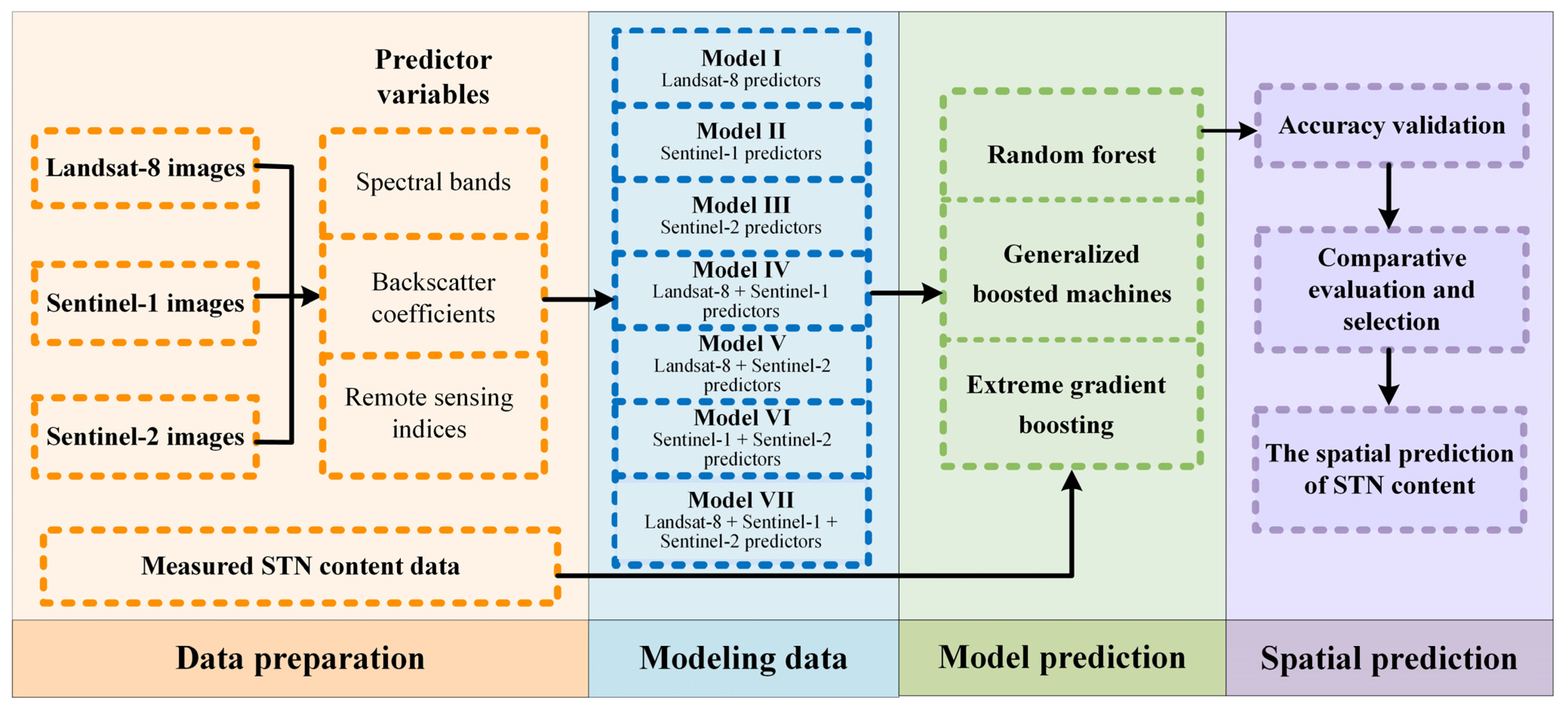
We constructed STN content models using three different machine learning methods and various combinations of predictor variables. The combinations of the different factors are shown in Table 4. Model I, Model II, and Model III used Landsat-8-, Sentinel-1-, and Sentinel-2-derived predictors, respectively, to predict STN content. Model IV and Model V were combinations of Landsat-8-derived predictors with Sentinel-1- and Sentinel-2- derived predictors, respectively, and Model VI used a combination of Sentinel-1- and Sentinel-2-derived predictors. Model VII included all predictor variables. Figure 3 shows an overview of the flowchart for STN content mapping using these experimental models. For the predictive performance of these models, we used a 10-fold cross-validation method [45]. For the 10-fold cross-validation, we randomly divided the observed dataset into 10 groups [46]. In each of the 10 folds, one group was designated as the test dataset and the other nine groups were used as the training set [47]. Three validation criteria were calculated to evaluate the performance of the model: the RMSE, the mean absolute error (MAE), and the coefficient of determination (R2). These validation criteria are calculated from the following [25]:
R 2 = i = 1 n y ^ l y ¯ 2 i = 1 n y i y ¯ 2
R M S E = 1 n i = 1 n y ^ i y i 2
M A E = 1 n i = 1 n y ^ l y i
where n represents the number of samples, y ^ l and y i represent the predicted and observed values at site i, respectively, and y ¯ represent the mean of observed values.

3. Results

3.1. Model Evaluation and Comparison

The performances of the RF, GBM, and XGBoost methods based on different combinations of predicting STN content are shown in Table 5. The different methods and variable combinations significantly affected the modeling performance. For the RF and GBM methods, Model I (R2 = 0.446 vs. R2 = 0.410, respectively), Model II (R2 = 0.411 vs. R2 = 0.391, respectively), and Model III (R2 = 0.409 vs. R2 = 0.394, respectively) were better predicted by the RF, indicating that the RF method is better than GBM in predicting STN content using single-type remote sensing data. However, the GBM method performed better than RF in Model IV (R2 = 0.479 vs. R2 = 0.459, respectively), Model V (R2 = 0.496 vs. R2 = 0.463, respectively), Model VI (R2 = 0.488 vs. R2 = 0.457, respectively), and Model VII (R2 = 0.533 vs. R2 = 0.475, respectively), indicating that the GBM method is more suitable than RF for predicting STN content using multiple source remote sensing data. Among the three machine learning methods, whether using single or multiple data types as prediction variables, the XGBoost method has the highest prediction accuracy for STN content.
When comparing different combinations of predictive variables, Model I (R2 = 0.446 and R2 = 0.410 for RF and GBM methods, respectively) performed better than Model II (R2 = 0.411 and R2 = 0.391 for the RF and GBM methods, respectively) and Model III (R2 = 0.409 and R2 = 0.394 for the RF and GBM methods, respectively), indicating that Landsat-8 images have a better predictive capability than the Sentinel-1 and Sentinel-2 images when modeling using the RF and GBM methods; Model II and Model III have similar prediction levels, indicating that Sentinel-1 and Sentinel-2 images have similar predictive capabilities. For the models that were established using the XGBoost method, the R2 of Model I and Model III is 15.5% (from 0.431 to 0.498) and 21.6% (from 0.431 to 0.524) higher than that of Model II, respectively, indicating that optical imagery performs better than SAR imagery. When compared with single-type remote sensing data, the combination of different types of data can improve prediction accuracy, and the addition of each type of data has a different degree of improvement in model accuracy. For example, when Sentinel-1 and Sentinel-2 predictors were added to Model I to form Model IV and Model V, the highest R2 increased by 16.83% and 20.98%, respectively. When Sentinel-2 predictors were added to Model II to form Model VI, the highest R2 increased by 37.5%. This indicates that the added data contain valuable information that is different from the original data. This improvement is similar across all three machine learning methods.
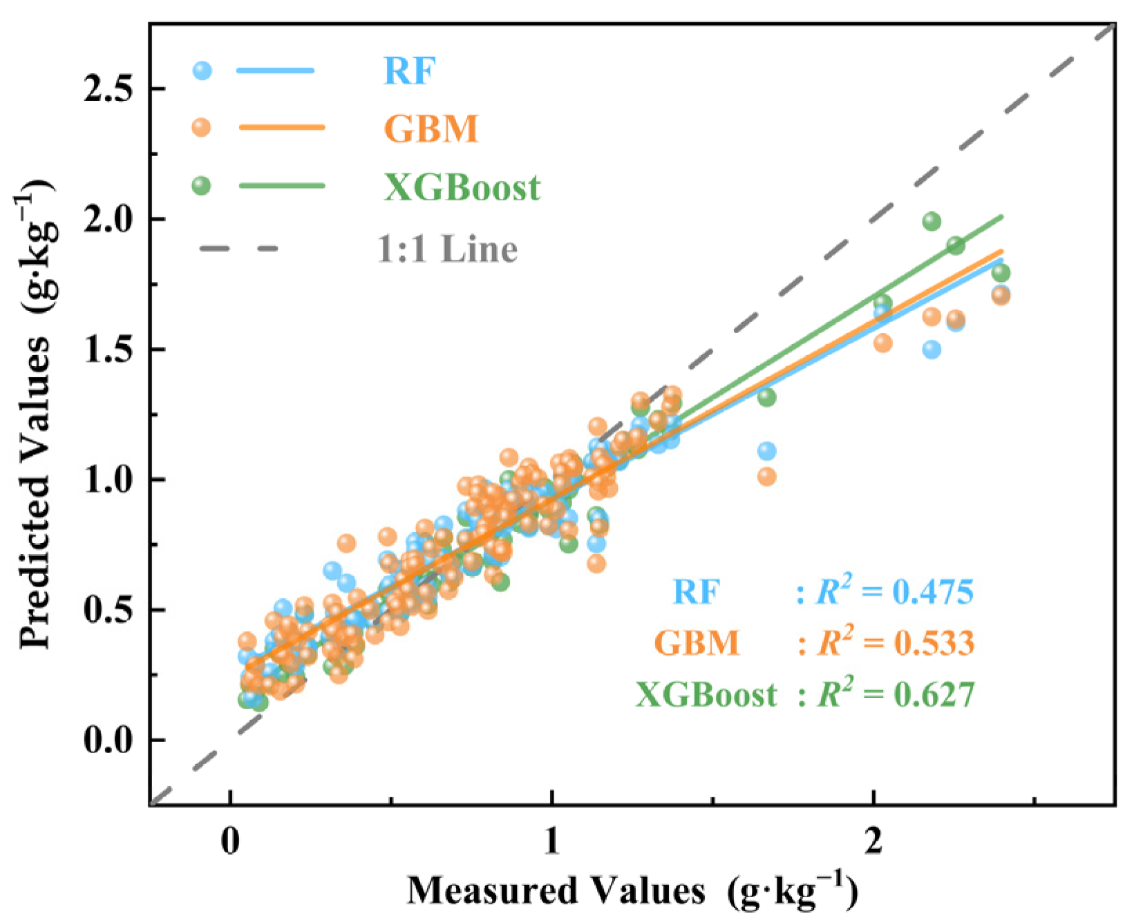
The models built using all prediction factors have the highest prediction accuracy. Model VII, which combines three types of remote sensing data as prediction factors, showed the most significant improvement. For example, when compared to Model II and constructed from a single data source, Model VII, based on the XGBoost method, improved the R2 value from 0.431 to 0.627, an increase of 45.48% compared to Model IV, which combines two types of data. The R2 value of Model VII (0.627) is 15.05% higher than that of Model IV (0.545). Model VII is based on three methods (R2 = 0.475, R2 = 0.533, and R2 = 0.627 for the RF, GBM, and XGBoost methods, respectively), which can explain the variation in STN content of 47.5%, 53.3%, and 62.7%, respectively. From the distribution of the measured value and the predicted value scatterplot (Figure 4), the STN content predicted by the XGBoost method is closer to the measured value, and the fitted straight line between the measured value and the predicted value is closer to the 1:1 line, followed by GBM, and RF is the worst.

3.2. Relative Importance of Variables

Model VII was built based on three machine learning methods using a combination of all predictive variables. The predictive variables sorted by relative importance are shown in Figure 5 (percentages were used to enhance comparability). Variables with less than 1% importance are not displayed in the graph, as they may be due to chance. Variables are ranked roughly the same in importance. For example, six out of the top nine important variables were duplicated in the GBM and XGBoost methods, namely VV, L_B5, S_NDVIRE2, VH, S_NDVIRE3, and S_B5. Five duplicated variables were found in the RF and XGBoost methods, namely L_NDWI, S_NDVIRE2, L_B5, VH, and VV. L_NDWI were the most significant explanatory variables in both models, accounting for 14.24% and 21.44% of the relative importance in predicting STN content. Four variables were duplicated among the top nine most important variables in all three methods, namely, VV, L_B5, S_NDVIRE2, and VH.
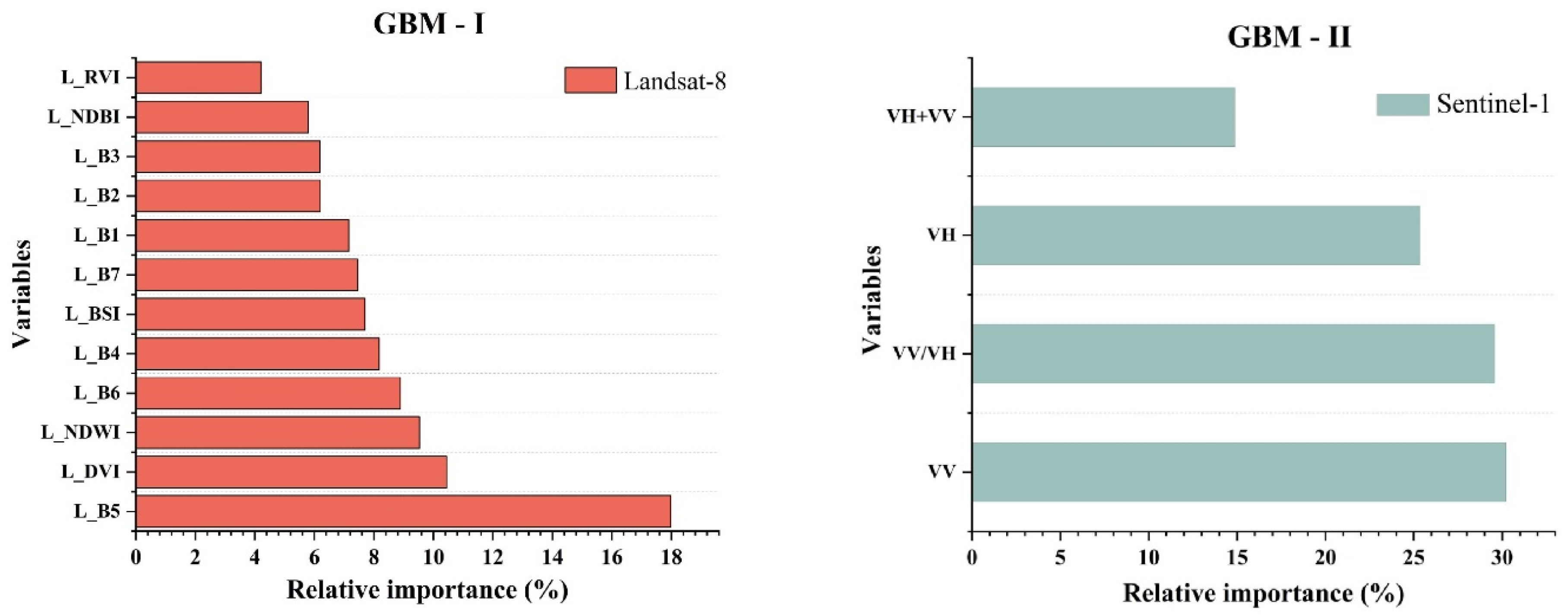
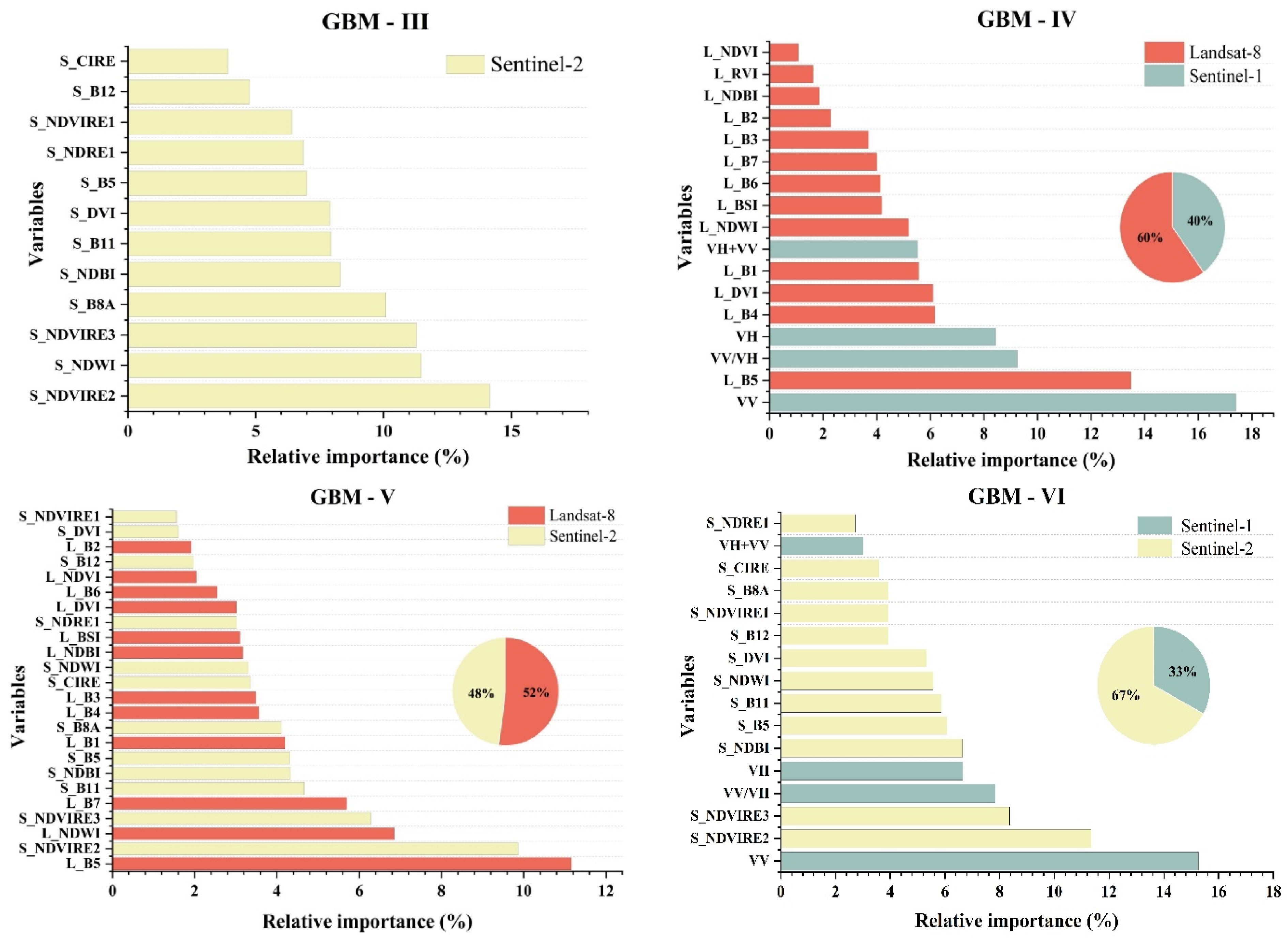
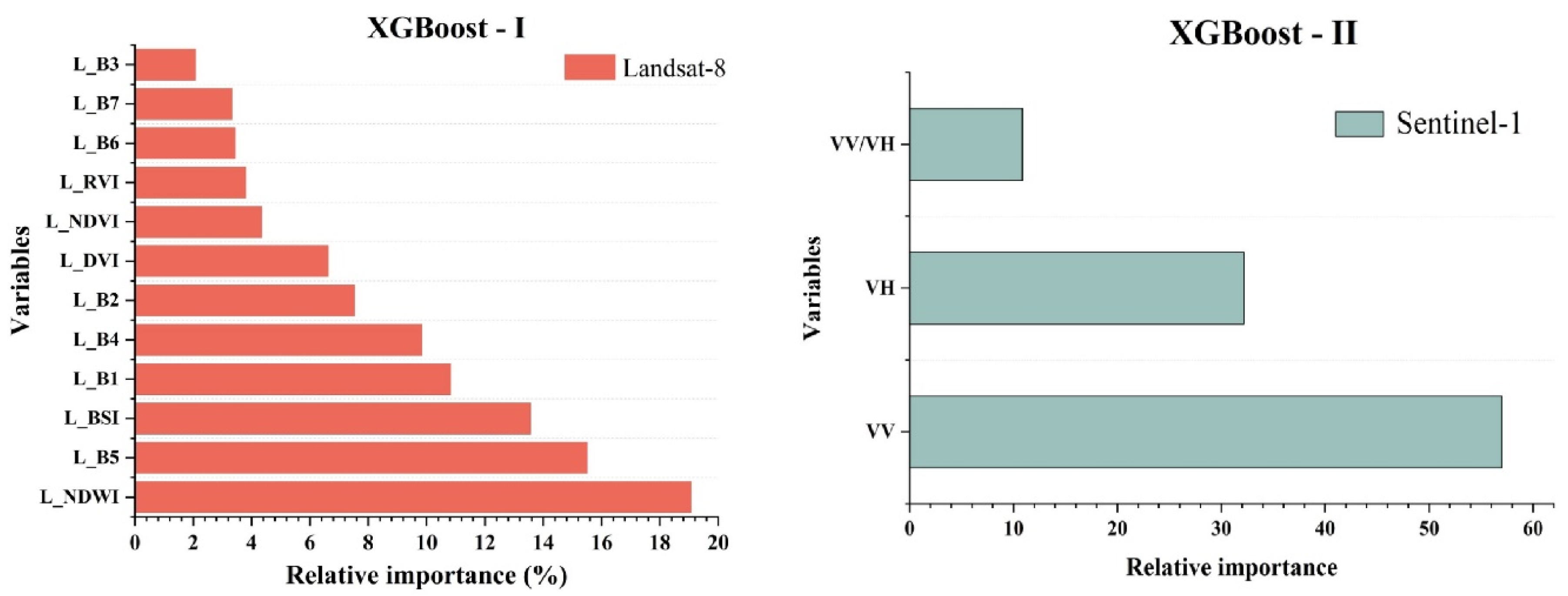
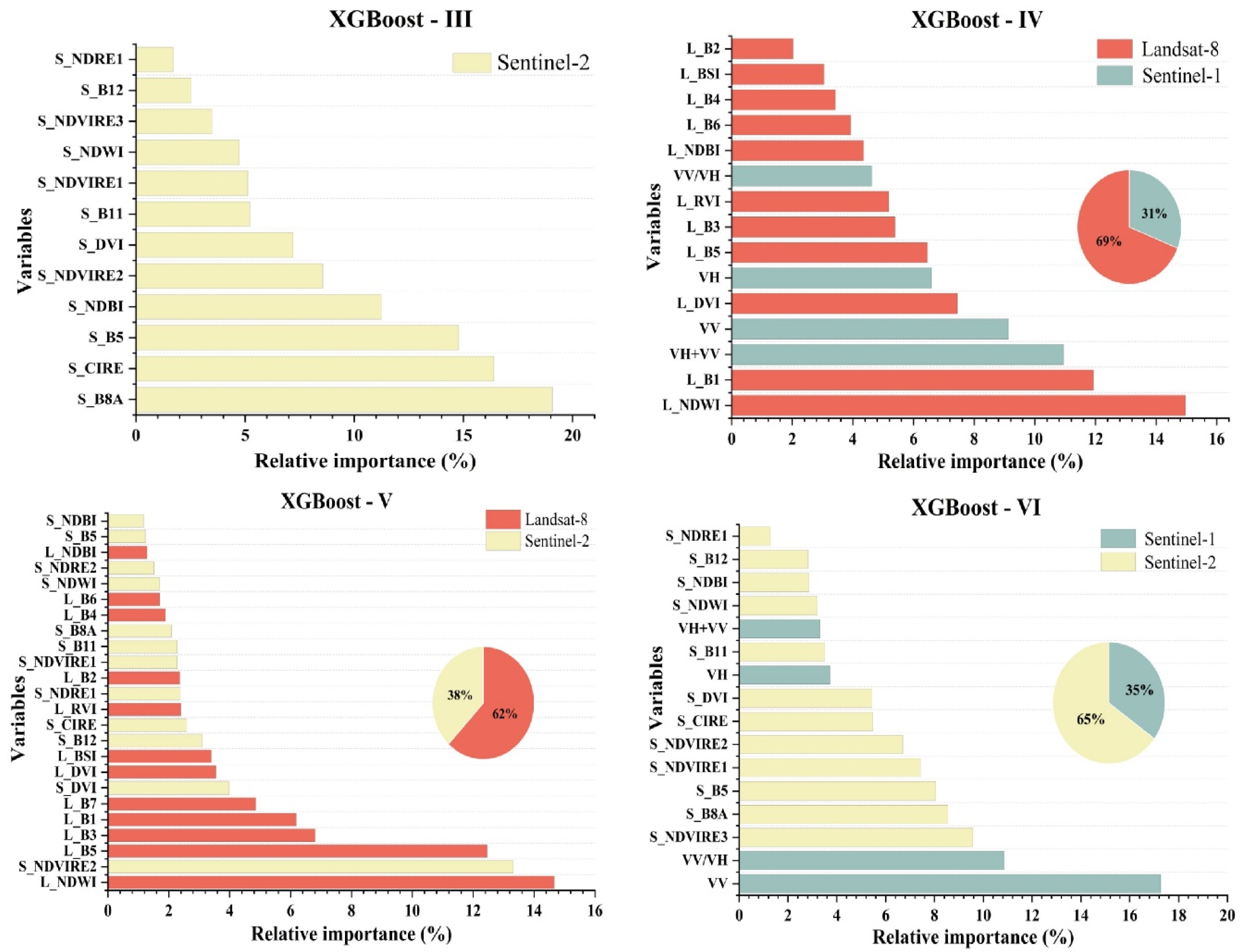
Model VII, which was constructed using the RF method, showed that Landsat-8 imagery (relative importance of 63%) is the main explanatory variable for STN content, followed by Sentinel-2 (24%) and Sentinel-1 (13%). Similarly, the XGBoost method-established Model VII also indicates that Landsat-8 has the highest relative importance (44%), followed by Sentinel-2 (33%), and Sentinel-1 has the lowest importance (23%). This suggests that Landsat-8 imagery has a stronger explanatory power for STN content than Sentinel series imagery for both the RF and XGBoost methods. However, GBM method-established Model VII, Landsat-8, and Sentinel-2 have similar explanatory powers. For all the models established using the RF, GBM, and XGBoost methods, the relative importance of Sentinel-1 is the lowest, at 13%, 24%, and 23%, respectively. This indicates that optical imagery is more helpful for predicting STN content. The same rules were observed in others, from Model Ⅰ to Model Ⅵ (Figure A1, Figure A2 and Figure A3).

3.3. Spatial Distribution Pattern of STN Content

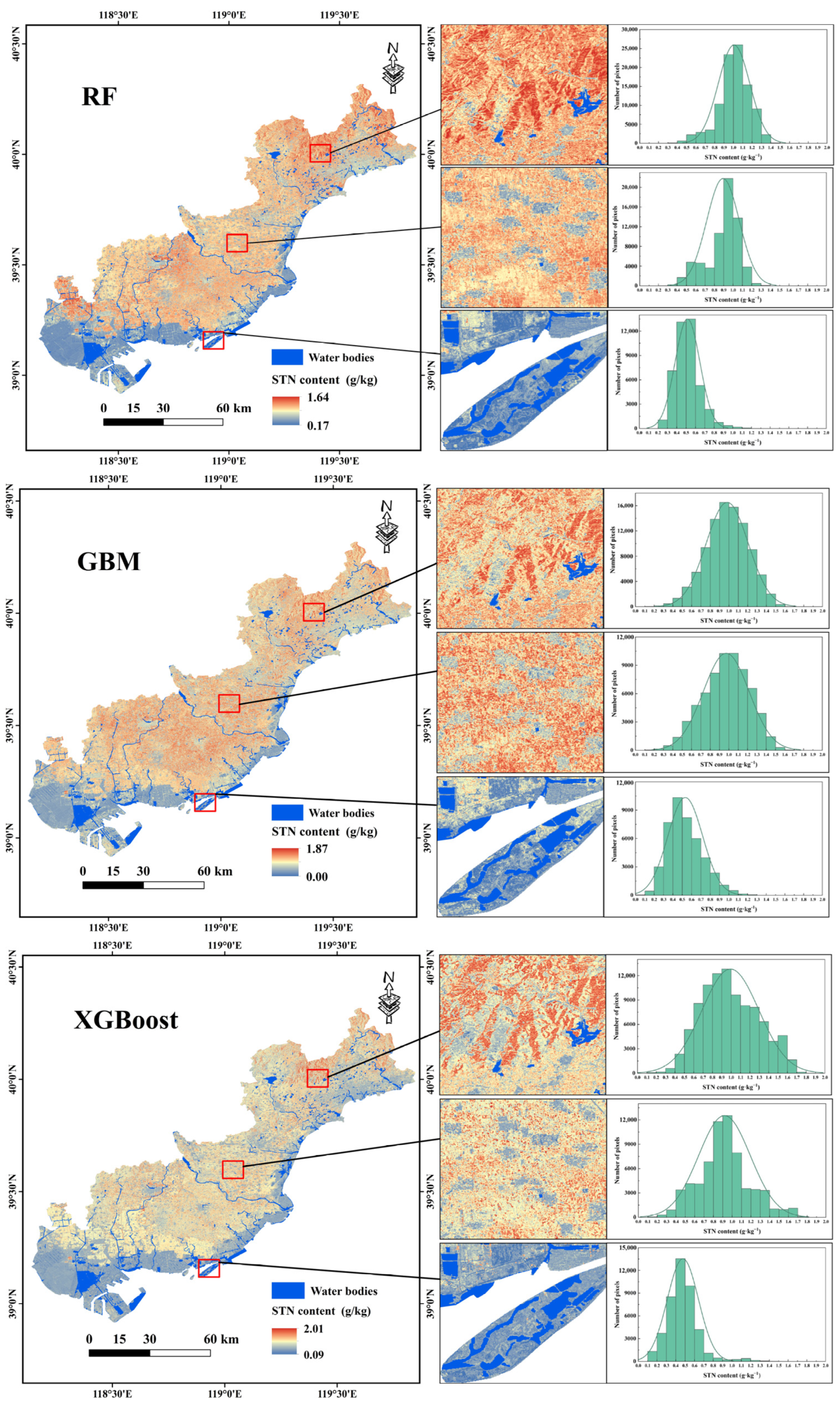
Based on the RF, GBM, and XGBoost methods, the established Model VII was selected to predict the STN content in the entire study area, and a spatial distribution map of the STN content in the study area was drawn (Figure 6). The spatial patterns of STN content predicted by the three methods are similar, and a strong spatial heterogeneity for STN content was observed on all of the distribution maps, with higher STN content in the northern part of the study area and lower content in coastal areas. Based on the statistical analysis, the predicted STN contents from different models show similarities. For instance, in coastal areas, the majority of the pixels have STN contents ranging from 0.4–0.5 g·kg−1. As we move from coastal wetlands to farmland areas to mountainous areas, the peak of the distribution curve shifts towards higher STN contents, indicating that the STN content in inland areas is significantly higher than that in coastal areas.
The three methods predict STN content in the study area, and the descriptive statistics are shown in Table 6. The SD values for STN content predicted by the RF model are lower than that predicted by GBM and XGBoost, indicating the robustness of the RF model is the highest. The predicted average STN content of each model is higher than the actual value.

4. Discussion

4.1. Accuracy and Influencing Factors of STN Content Prediction Models

The results demonstrate that the prediction methods, different types of data, and different combinations of data significantly influence the STN content predictive accuracy. The study did not find that the RF method-established models consistently outperformed GBM in predicting STN content using different variable combinations. Therefore, it is necessary to calibrate and evaluate competitive prediction models based on specific experimental datasets under different model combinations. The XGBoost method outperforms the RF and GBM methods in terms of prediction accuracy, a finding supported by Tien Dat Pham’s research [27]. However, Zhang et al. used RF, GBM, and XGBoost to study STN content in tobacco planting areas and found that GBM performed the best, followed by RF, with XGBoost performing the worst [48]. Some scholars have found that the three methods perform similarly [49]. This discrepancy may be due to differences in STN sample quantity as well as the types of remote sensing variables used. There is no consistent conclusion about the model performance of the RF, GBM, and XGBoost methods. It seems that no single machine learning method is most suitable for all ecosystems, so it is important to choose different methods based on different regions and remote sensing variables. As the RF method calculates an average value of the output values from multiple trees as the model’s prediction result, it is not sensitive to outliers [50]. This means that the RF method ignores the effect of extremely high or low STN content values on the prediction of STN content in the study area, resulting in a small predicted range for STN content in the entire region. GBM and XGBoost are both iterative models, with each model’s prediction based on the residuals of the previous model. The models are sensitive to outliers, as a large outlier may affect the residuals of each model and result in a wider predicted range of STN content [51]. Based on measured soil data, the STN content ranged from 0.052 to 2.396 g·kg−1. Among the three machine learning algorithms used in this study, the XGBoost method was found to be more accurate, supporting the results that XGBoost has better accuracy.
Our research findings demonstrate the crucial importance of three types of remote sensing imagery, namely Landsat-8, Sentinel-1, and Sentinel-2, in predicting STN content. The accuracy of the model based on the derived variables extracted from different remote sensing images is different. Although both Landsat-8 and Sentinel-2 are optical remote sensing images, the information contained in the images is different due to differences in their center wavelength, bandwidth, and overlapping bands [15], and the difference in image acquisition time also leads to differences in the information contained in the images [52], which can lead to different prediction capabilities for STN content. The models (Model II) based on Sentinel-1-derived variables had lower accuracy compared to the models (Model I and Model III) based on optical image-derived variables. This suggests that the predictive ability of optical images is superior to SAR images in the study area, which is consistent with previous research [53]. However, the Sentinel-1 data helped to improve the accuracy of the models, and the study found that when the predictors extracted from SAR images were added, the model accuracy improved, indicating that Sentinel-1 imagery contains useful information beyond Landsat-8 and Sentinel-2 [15]. There is a study that found the inclusion of Sentinel-1 imagery improves the model accuracy, contributing 9% and 7% to the RF and BRT models, respectively, supporting the results of this experiment [53]. The inclusion of different sensor data in the model significantly improved its accuracy, indicating that Landsat 8, Sentinel-1, and Sentinel-2 images contain different valuable information. Previous studies on predicting soil properties mainly used a single sensor, such as Landsat [54] and Sentinel-2 [35,45], without considering the feasibility of radar sensors. In this study, the better prediction accuracy obtained from the combination of optical and SAR images demonstrates the usefulness of SAR data in predicting STN content. The combination of optical and radar sensors has great potential in predicting soil properties [55].
Among all the prediction models, Model VII, based on the XGBoost method, has the highest prediction accuracy and can explain 62.7% of the variability in STN content. Our prediction model has achieved higher accuracy compared to other scholars’ predictions of STN content. For example, Wadoux et al. established an RF model using French LUCAS data, which can only explain 20% of the variability in STN content [54]. ZHOU et al. used data from the Second National Land Survey from 1979 to 1985 to construct XGBoost, RF, and weighted model averaging methods to predict STN content across China, with R2 values of 0.34, 0.38, and 0.41, respectively [56]. Although public soil datasets have wide coverage and rich attribute information for the sampling points, they have poor timelines due to their long sampling time and cannot be matched with recent remote sensing images, thus, they can only be used to invert soil properties during the sampling period. When compared to using public datasets, field sampling provides controllable data for specific experiments, with the spatial and temporal consistency between the samples and remote sensing images being the most important advantage, which had a certain effect on improving the accuracy of the model.

4.2. Relative Importance of Variables

In this study, among the RF, GBM, and XGBoost method-established optimal models, the prediction factors provided by Landsat-8 data accounted for 63%, 37%, and 44% of the importance of all variables, respectively. The prediction factors provided by Sentinel-2 data accounted for 24%, 39%, and 33% of the importance of all variables, respectively. The prediction factors provided by Sentinel-1 data accounted for 13%, 24%, and 23% of the importance of all variables, respectively. It can be seen that optical images are the most important in explaining the variability of STN content. Among the two optical images, Landsat-8 has greater importance than Sentinel-2 in all but the GBM prediction results, where their importance is similar. This suggests that Landsat-8 data have a greater impact on the study area than Sentinel-2. Additionally, when compared to optical images, SAR images have lower importance in predicting STN content. This result is supported by the study of Zhou et al. [53].
The spectral bands, the remote sensing indices of optical imagery, and the backscatter coefficients of radar imagery are extracted through remote sensing images to help explain the spatial variation in STN content in the soil-vegetation system. They can capture the relationship between soil properties and vegetation to reflect soil information to some extent. Remote sensing images represent a valuable dataset for explaining spatial changes in the soil in natural vegetation areas [57]. In the RF, GBM, and XGBoost prediction models, remote sensing indices accounted for 69%, 45%, and 55% of the model’s contribution, respectively. Remote sensing indices contribute more to the models than band reflectance. Specifically, in the RF and XGBoost models, remote sensing indices have a higher contribution rate than band reflectance, indicating that remote sensing indices can better characterize soil information and have higher values for the prediction of STN content. In addition, band reflectance is more important than remote sensing indices in GBM models, indicating that the role of band reflectance is relatively more important in the GBM model. In the RF and XGBoost models, the importance of NDWI is highest, and soil moisture promotes the accumulation of ecosystem STN content [58]. Xu’s research also proves that NDWI strongly correlates with STN content [33]. The sampling sites in this study are mostly located in intertidal flats, paddy fields, and marsh land cover types, where soil moisture is high, which is expected to result in the high importance of NDWI. Remote sensing images are more sensitive to vegetation and are indirectly sensitive to soil properties; the data were collected from September to October, when vegetation was flourishing, and the calculated vegetation indices were relatively high. The importance of vegetation indices is high in this study, among which the red edge index S_NDVIRE2 has a large contribution to the models. The red edge indices are recognized as the most suitable remote sensing indices for reflecting vegetation growth [59], which means that they can estimate soil properties better through the vegetation medium. This view is also supported in this study.

4.3. Spatial Distribution of STN Content

The spatial distribution of STN content predicted in this study is similar to that of the 0–20 cm STN content data set in China by Zhou et al. [56]. The spatial distribution of STN content predicted by the three modeling methods is also similar, further indicating that the results of this study are in line with reality. High levels of STN content were mainly distributed in the northern mountainous areas that were covered with dense vegetation. Correspondingly, low levels of STN content were mainly found in the southern and central regions that were dominated by high levels of human activity areas such as coastal and urban areas, indicating that areas with dense tree cover are more conducive to the accumulation of STN content, which is consistent with the results of Zhou et al. [60]. Cropland STN content is second only to the northern mountainous areas, which may be due to the fertilization of farmland, which causes some nitrogen elements to infiltrate into the soil [15,61]. In addition, a large amount of agricultural waste, residue, and feces will be produced during the agricultural production process, and these materials will degrade into organic matter and release nitrogen elements, further increasing the STN content [62]. In terms of the prediction results, the spatial distribution of STN based on the XGBoost method shows that the STN content ranges from 0 to 2.01 g·kg−1. These distribution ranges are consistent with those presented in the STN maps produced by Xu et al. [33] and Li et al. [63].
However, there are some uncertainties in our study. Firstly, time-series images provide more information compared to single-time remote sensing images, reduce uncertainty and improve model accuracy, and future studies might consider extracting time-series remote sensing variables for predicting STN content [18]. This study resampled the spatial resolution of all the remote sensing variables to 30 m without considering the impact of spatial resolution on modeling and inversion accuracy. However, different spatial resolutions can lead to different mixes of land features, thereby affecting the accuracy of the modeling and inversion. Therefore, it is crucial to determine an appropriate spatial resolution for predicting soil properties. In the next step of the research, we will pay attention to considering the impact of spatial resolution on soil property prediction and explore suitable strategies for selecting spatial resolution to enhance the accuracy and reliability of the model.

5. Conclusions

This study combined three commonly used remote sensing images, including two multispectral images (Landsat-8 and Sentinel-2) and one SAR image (Sentinel-1), and used three decision tree-based machine learning methods (RF, GBM, and XGBoost) to predict the STN content in a coastal area. The spatial distribution of the STN content was mapped. Our conclusions are summarized as follows:
  • The application of SAR and optical images proved useful for predicting STN content, and their combination showed enhanced model accuracy. The RF, GBM, and XGBoost methods demonstrated maximum improvements of 16%, 36%, and 45%, respectively;
  • The XGBoost method had higher accuracy than the RF and GBM methods. The optimal model was built using the XGBoost method, with an R2 of 0.627, RMSE of 0.127 g·kg−1, and an MAE of 0.092 g·kg−1;
  • Optical imagery is more helpful than SAR imagery in predicting STN content. In the models established by the RF and XGBoost methods, Landsat-8 had the highest relative importance (63% and 44%, respectively), followed by Sentinel-2 (24% and 33%, respectively). In the model established by the GBM method, the importance of Landsat-8 and Sentinel-2 was similar but higher than that of Sentinel-1;
  • The STN content predicted by the three models has a certain degree of similarity for spatial distribution. The predicted range of STN content is from 0 to 2.01 g·kg−1. These maps showed significant spatial variability. The STN content is high in the densely forested areas in the north and low in the paddy wetlands in the southeast.

Author Contributions

Conceptualization, Q.Z., F.W., Y.Z., D.M., M.L. and J.S.; methodology, Q.Z., Y.Z., W.M., M.L. and D.M.; software, Q.Z., J.S. and X.L.; validation, W.M., M.L. and F.W.; formal analysis, W.M. and M.L.; investigation, Q.Z.; resources, C.K. and C.L.; data curation, Q.Z., X.L. and C.K.; writing—original draft preparation, Q.Z. and W.M.; writing—review and editing, W.M. and M.L.; visualization, Q.Z., X.L. and C.K.; supervision, Y.Z. and F.L.; project administration, W.M.; funding acquisition, W.M., M.L. and Y.Z. All authors have read and agreed to the published version of the manuscript.

Funding

This research was funded by the National Natural Science Foundation of China (Grant No. 41901375, 42101393, and 52274166), the Natural Science Foundation of Hebei Province, China (Grant No. D2022209005, D2019209322 and D2019209317), the Funding Project for the Introduction of Returned Overseas Chinese Scholars of Hebei, China (Grant No. C20200103), Funded by Science and Technology Project of Hebei Education Department (Grant No. BJ2020058), the Key Research and Development Program of Science and Technology Plan of Tangshan, China (Grant No. 22150221J), the North China University of Science and Technology Foundation (Grant No. BS201824 and BS201825), the Fostering Project for Science and Technology Research and Development Platform of Tangshan, China (No. 2020TS003b).

Data Availability Statement

The data presented in this study are available on request from the corresponding author. The data are not publicly available due to privacy restrictions.

Acknowledgments

The authors would like to thank Yufeng Hao, Kuo Zhang, Mimi Gao, Xiaowu Yang, Hao Zheng, Yahui Liu, Chunyu Li, and Tanglei Song for collecting soil samples. The authors are deeply grateful to the anonymous reviewers and the editor for their helpful comments on the manuscript.

Conflicts of Interest

The authors declare no conflict of interest.

Appendix A

Figure A1. Relative importance of variables used for the STN content prediction in Model I to Model Ⅵ based on RF method.
Remotesensing 15 02907 g0a1aRemotesensing 15 02907 g0a1b
Figure A2. Relative importance of variables used for the STN content prediction in Model I to Model Ⅵ based on GBM method.
Remotesensing 15 02907 g0a2aRemotesensing 15 02907 g0a2b
Figure A3. Relative importance of variables used for the STN content prediction in Model I to Model Ⅵ based on XGBoost method.
Remotesensing 15 02907 g0a3aRemotesensing 15 02907 g0a3b

References

  1. Wang, Y.; Zhang, X.; Huang, C. Spatial variability of soil total nitrogen and soil total phosphorus under different land uses in a small watershed on the Loess Plateau, China. Geoderma 2009, 150, 141–149. [Google Scholar] [CrossRef]
  2. Zhang, Y.; Li, M.; Zheng, L.; Qin, Q.; Lee, W.S. Spectral features extraction for estimation of soil total nitrogen content based on modified ant colony optimization algorithm. Geoderma 2019, 333, 23–34. [Google Scholar] [CrossRef]
  3. Sarker, S.; Veremyev, A.; Boginski, V.; Singh, A. Critical Nodes in River Networks. Sci. Rep. 2019, 9, 11178. [Google Scholar] [CrossRef] [Green Version]
  4. Batjes, N.H. Total carbon and nitrogen in the soils of the world. Eur. J. Soil Sci. 1996, 47, 151–163. [Google Scholar] [CrossRef]
  5. Mao, D.; Luo, L.; Wang, Z.; Wilson, M.C.; Zeng, Y.; Wu, B.; Wu, J. Conversions between natural wetlands and farmland in China: A multiscale geospatial analysis. Sci. Total Environ. 2018, 634, 550–560. [Google Scholar] [CrossRef] [PubMed]
  6. Gao, Y.; Sarker, S.; Sarker, T.; Leta, O.T. Analyzing the critical locations in response of constructed and planned dams on the Mekong River Basin for environmental integrity. Environ. Res. Commun. 2022, 4, 101001. [Google Scholar] [CrossRef]
  7. Yang, L.; Luo, P.; Wen, L.; Li, D. Soil organic carbon accumulation during post-agricultural succession in a karst area, southwest China. Sci. Rep. 2016, 6, 37118. [Google Scholar] [CrossRef] [PubMed]
  8. Yang, R.; Zhang, G.; Yang, F.; Yang, Y.; Yang, D. Comparison of boosted regression tree and random forest models for mapping topsoil organic carbon concentration in an alpine ecosystem. Ecol. Indic. 2016, 60, 870–878. [Google Scholar] [CrossRef]
  9. Jeong, G.; Oeverdieck, H.; Park, S.J.; Huwe, B.; Ließ, M. Spatial soil nutrients prediction using three supervised learning methods for assessment of land potentials in complex terrain. Catena 2017, 154, 73–84. [Google Scholar] [CrossRef]
  10. Minasny, B.; McBratney, A.B. Digital soil mapping: A brief history and some lessons. Geoderma 2016, 264, 301–311. [Google Scholar] [CrossRef]
  11. Forkuor, G.; Hounkpatin, O.K.L.; Welp, G.; Thiel, M. High Resolution Mapping of Soil Properties Using Remote Sensing Variables in South-Western Burkina Faso: A Comparison of Machine Learning and Multiple Linear Regression Models. PLoS ONE 2017, 12, e0170478. [Google Scholar] [CrossRef] [PubMed] [Green Version]
  12. Bhattarai, N.; Quackenbush, L.J.; Dougherty, M.; Marzen, L.J. A simple Landsat–MODIS fusion approach for monitoring seasonal evapotranspiration at 30 m spatial resolution. Int. J. Remote Sens. 2015, 36, 115–143. [Google Scholar] [CrossRef]
  13. Siqueira, R.G.; Moquedace, C.M.; Francelino, M.R.; Schaefer, C.E.G.R.; Fernandes-Filho, E.I. Machine learning applied for Antarctic soil mapping: Spatial prediction of soil texture for Maritime Antarctica and Northern Antarctic Peninsula. Geoderma 2023, 432, 116405. [Google Scholar] [CrossRef]
  14. Zhou, T.; Geng, Y.; Ji, C.; Xu, X.; Wang, H.; Pan, J.; Bumberger, J.; Haase, D.; Lausch, A. Prediction of soil organic carbon and the C:N ratio on a national scale using machine learning and satellite data: A comparison between Sentinel-2, Sentinel-3 and Landsat-8 images. Sci. Total Environ. 2020, 755, 142661. [Google Scholar] [CrossRef] [PubMed]
  15. Xu, Y.; Li, B.; Shen, X.; Li, K.; Cao, X.; Cui, G.; Yao, Z. Digital soil mapping of soil total nitrogen based on Landsat 8, Sentinel 2, and WorldView-2 images in smallholder farms in Yellow River Basin, China. Environ. Monit. Assess. 2022, 194, 282. [Google Scholar] [CrossRef] [PubMed]
  16. Poggio, L.; Gimona, A. Assimilation of optical and radar remote sensing data in 3D mapping of soil properties over large areas. Sci. Total Environ. 2017, 579, 1094–1110. [Google Scholar] [CrossRef] [Green Version]
  17. Kamran, A.; Younes, G.; Shamsollah, A.; Samaneh, T. Integration of Sentinel-1/2 and topographic attributes to predict the spatial distribution of soil texture fractions in some agricultural soils of western Iran. Soil Tillage Res. 2023, 229, 105681. [Google Scholar]
  18. Yang, R.; Guo, W. Using time-series Sentinel-1 data for soil prediction on invaded coastal wetlands. Environ. Monit. Assess. 2019, 191, 462. [Google Scholar] [CrossRef]
  19. Zare, S.; Fallah, S.S.R.; Abtahi, S.A. Weakly-coupled geo-statistical mapping of soil salinity to Stepwise Multiple Linear Regression of MODIS spectral image products. J. Afr. Earth Sci. 2019, 152, 101–114. [Google Scholar] [CrossRef]
  20. Xu, S.; Wang, M.; Shi, X.; Yu, Q.; Zhang, Z. Integrating hyperspectral imaging with machine learning techniques for the high-resolution mapping of soil nitrogen fractions in soil profiles. Sci. Total Environ. 2021, 754, 142135. [Google Scholar] [CrossRef]
  21. Karunaratne, S.B.; Bishop, T.F.A.; Baldock, J.A.; Odeh, I.O.A. Catchment scale mapping of measureable soil organic carbon fractions. Geoderma 2014, 219–220, 14–23. [Google Scholar] [CrossRef]
  22. Xu, Y.; Smith, S.E.; Grunwald, S.; Abd-Elrahman, A.; Wani, S.P.; Nair, V.D. Estimating soil total nitrogen in smallholder farm settings using remote sensing spectral indices and regression kriging. Catena 2018, 163, 111–122. [Google Scholar] [CrossRef] [Green Version]
  23. Westhuizen, S.v.d.; Heuvelink, G.B.M.; Hofmeyr, D.P. Multivariate random forest for digital soil mapping. Geoderma 2023, 431, 116365. [Google Scholar] [CrossRef]
  24. Gomes, L.C.; Faria, R.M.; Souza, E.d.; Veloso, G.V.; Schaefer, C.E.G.R.; Filho, E.I.F. Modelling and mapping soil organic carbon stocks in Brazil. Geoderma 2019, 340, 337–350. [Google Scholar] [CrossRef]
  25. Wang, S.; Adhikari, K.; Wang, Q.; Jin, X.; Li, H. Role of environmental variables in the spatial distribution of soil carbon (C), nitrogen (N), and C:N ratio from the northeastern coastal agroecosystems in China. Ecol. Indic. 2018, 84, 263–272. [Google Scholar] [CrossRef]
  26. Zhang, X.; Xue, J.; Chen, S.; Wang, N.; Shi, Z.; Huang, Y.; Zhuo, Z. Digital Mapping of Soil Organic Carbon with Machine Learning in Dryland of Northeast and North Plain China. Remote Sens. 2022, 14, 2504. [Google Scholar] [CrossRef]
  27. Pham, T.D.; Yokoya, N.; Nguyen, T.T.T.; Le, N.N.; Ha, N.T.; Xia, J.; Takeuchi, W.; Pham, T.D. Improvement of Mangrove Soil Carbon Stocks Estimation in North Vietnam Using Sentinel-2 Data and Machine Learning Approach. GIScience Remote Sens. 2021, 58, 68–87. [Google Scholar] [CrossRef]
  28. Yang, J.; Fan, J.; Lan, Z.; Mu, X.; Wu, Y.; Xin, Z.; Miping, P.; Zhao, G. Improved Surface Soil Organic Carbon Mapping of SoilGrids250m Using Sentinel-2 Spectral Images in the Qinghai–Tibetan Plateau. Remote Sens. 2023, 15, 114. [Google Scholar] [CrossRef]
  29. Lan, J.; Hu, N.; Fu, W. Soil carbon–nitrogen coupled accumulation following the natural vegetation restoration of abandoned farmlands in a karst rocky desertification region. Ecol. Eng. 2020, 158, 106033. [Google Scholar] [CrossRef]
  30. Bhunia, G.S.; Shit, P.K.; Pourghasemi, H.R. Soil organic carbon mapping using remote sensing techniques and multivariate regression model. Geocarto Int. 2019, 34, 215–226. [Google Scholar] [CrossRef]
  31. John, K.; Isong, I.A.; Kebonye, N.M.; Ayito, E.O.; Agyeman, P.C.; Afu, S.M. Using Machine Learning Algorithms to Estimate Soil Organic Carbon Variability with Environmental Variables and Soil Nutrient Indicators in an Alluvial Soil. Land 2020, 9, 487. [Google Scholar] [CrossRef]
  32. Wang, M.; Mao, D.; Xiao, X.; Song, K.; Jia, M.; Ren, C.; Wang, Z. Interannual changes of coastal aquaculture ponds in China at 10-m spatial resolution during 2016–2021. Remote Sens. Environ. 2023, 284, 113347. [Google Scholar] [CrossRef]
  33. Xu, Y.; Wang, X.; Bai, J.; Wang, D.; Wang, W.; Guan, Y. Estimating the spatial distribution of soil total nitrogen and available potassium in coastal wetland soils in the Yellow River Delta by incorporating multi-source data. Ecol. Indic. 2020, 111, 106002. [Google Scholar] [CrossRef]
  34. Liu, Y.; Qian, J.; Yue, H. Comprehensive Evaluation of Sentinel-2 Red Edge and Shortwave-Infrared Bands to Estimate Soil Moisture. IEEE J. Sel. Top. Appl. Earth Obs. Remote Sens. 2021, 14, 7448–7465. [Google Scholar] [CrossRef]
  35. Nabiollahi, K.; Taghizadeh-Mehrjardi, R.; Shahabi, A.; Heung, B.; Scholten, T. Assessing agricultural salt-affected land using digital soil mapping and hybridized random forests. Geoderma 2021, 385, 114858. [Google Scholar] [CrossRef]
  36. Taghizadeh-Mehrjardi, R.; Schmidt, K.; Amirian-Chakan, A.; Rentschler, T.; Zeraatpisheh, M.; Sarmadian, F.; Valavi, R.; Davatgar, N.; Behrens, T.; Scholten, T. Improving the Spatial Prediction of Soil Organic Carbon Content in Two Contrasting Climatic Regions by Stacking Machine Learning Models and Rescanning Covariate Space. Remote Sens. 2020, 12, 1095. [Google Scholar] [CrossRef] [Green Version]
  37. Bremner, J.M. Determination of nitrogen in soil by the Kjeldahl method. J. Agric. Sci. 1960, 55, 11–33. [Google Scholar] [CrossRef]
  38. Fathololoumi, S.; Vaezi, A.R.; Alavipanah, S.K.; Ghorbani, A.; Biswas, A. Effect of multi-temporal satellite images on soil moisture prediction using a digital soil mapping approach. Geoderma 2021, 385, 114901. [Google Scholar] [CrossRef]
  39. Song, J.; Gao, J.; Zhang, Y.; Li, F.; Man, W.; Liu, M.; Wang, J.; Li, M.; Zheng, H.; Yang, X.; et al. Estimation of Soil Organic Carbon Content in Coastal Wetlands with Measured VIS-NIR Spectroscopy Using Optimized Support Vector Machines and Random Forests. Remote Sens. 2022, 14, 4372. [Google Scholar] [CrossRef]
  40. Hamzehpour, N.; Shafizadeh-Moghadam, H.; Valavi, R. Exploring the driving forces and digital mapping of soil organic carbon using remote sensing and soil texture. Catena 2019, 182, 104141. [Google Scholar] [CrossRef]
  41. Ridgeway, G. gbm: Generalized boosted regression models. R Package Version 2006, 1, 55. [Google Scholar]
  42. Jia, Y.; Jin, S.; Savi, P.; Gao, Y.; Tang, J.; Chen, Y.; Li, W. GNSS-R Soil Moisture Retrieval Based on a XGboost Machine Learning Aided Method: Performance and Validation. Remote Sens. 2019, 11, 1655. [Google Scholar] [CrossRef] [Green Version]
  43. Li, Y.; Zeng, H.; Zhang, M.; Wu, B.; Zhao, Y.; Yao, X.; Cheng, T.; Qin, X.; Wu, F. A county-level soybean yield prediction framework coupled with XGBoost and multidimensional feature engineering. Int. J. Appl. Earth Obs. Geoinf. 2023, 118, 103269. [Google Scholar] [CrossRef]
  44. Kuhn, M.; Johnson, K. Applied Predictive Modeling; Springer: Berlin/Heidelberg, Germany, 2013; Volume 26. [Google Scholar]
  45. Taghizadeh-Mehrjardi, R.; Nabiollahi, K.; Kerry, R. Digital mapping of soil organic carbon at multiple depths using different data mining techniques in Baneh region, Iran. Geoderma 2016, 266, 98–110. [Google Scholar] [CrossRef]
  46. Aitkenhead, M.J. Mapping peat in Scotland with remote sensing and site characteristics. Eur. J. Soil Sci. 2017, 68, 28–38. [Google Scholar] [CrossRef] [Green Version]
  47. Ottoy, S.; Vos, B.D.; Sindayihebura, A.; Hermy, M.; Orshoven, J.V. Assessing soil organic carbon stocks under current and potential forest cover using digital soil mapping and spatial generalisation. Ecol. Indic. 2017, 77, 139–150. [Google Scholar] [CrossRef]
  48. Zhang, X.; Yang, C.; Liu, H.; Wu, W. Predictions on organic matter and total nitrogen contents in tobacco-growing soil based on machine learning. Tob. Sci. Technol. 2022, 55, 20–27. (In Chinese) [Google Scholar] [CrossRef]
  49. Ghosh, S.M.; Behera, M.D.; Jagadish, B.; Das, A.K.; Mishra, D.R. A novel approach for estimation of aboveground biomass of a carbon-rich mangrove site in India. J. Environ. Manag. 2021, 292, 112816. [Google Scholar] [CrossRef]
  50. Wang, S.; Jin, X.; Adhikari, K.; Li, W.; Yu, M.; Bian, Z.; Wang, Q. Mapping total soil nitrogen from a site in northeastern China. Catena 2018, 166, 134–146. [Google Scholar] [CrossRef]
  51. Salunke, R.; Nobahar, M.; Alzeghoul, O.E.; Khan, S.; La Cour, I.; Amini, F. Near-Surface Soil Moisture Characterization in Mississippi’s Highway Slopes Using Machine Learning Methods and UAV-Captured Infrared and Optical Images. Remote Sens. 2023, 15, 1888. [Google Scholar] [CrossRef]
  52. Castaldi, F.; Chabrillat, S.; Don, A.; Wesemael, B.v. Soil Organic Carbon Mapping Using LUCAS Topsoil Database and Sentinel-2 Data: An Approach to Reduce Soil Moisture and Crop Residue Effects. Remote Sens. 2019, 11, 2121. [Google Scholar] [CrossRef] [Green Version]
  53. Zhou, T.; Geng, Y.; Chen, J.; Liu, M.; Haase, D.; Lausch, A. Mapping soil organic carbon content using multi-source remote sensing variables in the Heihe River Basin in China. Ecol. Indic. 2020, 114, 106288. [Google Scholar] [CrossRef]
  54. Wadoux, A.M.J.-C. Using deep learning for multivariate mapping of soil with quantified uncertainty. Geoderma 2019, 351, 59–70. [Google Scholar] [CrossRef] [Green Version]
  55. Li, Z.; Liu, F.; Peng, X.; Hu, B.; Song, X. Synergetic use of DEM derivatives, Sentinel-1 and Sentinel-2 data for mapping soil properties of a sloped cropland based on a two-step ensemble learning method. Sci. Total Environ. 2023, 866, 161421. [Google Scholar] [CrossRef] [PubMed]
  56. Zhou, Y.; Xue, J.; Chen, S.; Zho, Y.; Liang, Z.; Wang, N.; Shi, Z. Fine-Resolution Mapping of Soil Total Nitrogen across China Based on Weighted Model Averaging. Remote Sens. 2020, 12, 85. [Google Scholar] [CrossRef] [Green Version]
  57. Yang, R.; Guo, W. Modelling of soil organic carbon and bulk density in invaded coastal wetlands using Sentinel-1 imagery. Int. J. Appl. Earth Obs. Geoinf. 2019, 82, 101906. [Google Scholar] [CrossRef]
  58. Wang, J.; Bai, J.; Zhao, Q.; Lu, Q.; Xia, Z. Five-year changes in soil organic carbon and total nitrogen in coastal wetlands affected by flow-sediment regulation in a Chinese delta. Sci. Rep. 2016, 6, 21137. [Google Scholar] [CrossRef] [PubMed] [Green Version]
  59. Guo, Y.; Liu, Y.; Xu, M.; Zhang, X. Modeling and analysis of red edge index estimated by leaf area index in road vagetation. Sci. Surv. Mapp. 2021, 46, 93–98. [Google Scholar] [CrossRef]
  60. Zhou, T.; Geng, Y.; Chen, J.; Pan, J.; Haase, D.; Lausch, A. High-resolution digital mapping of soil organic carbon and soil total nitrogen using DEM derivatives, Sentinel-1 and Sentinel-2 data based on machine learning algorithms. Sci. Total Environ. 2020, 729, 138244. [Google Scholar] [CrossRef] [PubMed]
  61. Zhang, H.; Wu, P.; Yin, A.; Yang, X.; Zhang, X.; Zhang, M.; Gao, C. Organic carbon and total nitrogen dynamics of reclaimed soils following intensive agricultural use in eastern China. Agric. Ecosyst. Environ. 2016, 235, 193–203. [Google Scholar] [CrossRef]
  62. Magalhães, T.M.; Mamugy, F.P.S. Fine root biomass and soil properties following the conversion of miombo woodlands to shifting cultivation lands. Catena 2020, 194, 104693. [Google Scholar] [CrossRef]
  63. Li, X.; Shang, B.; Wang, D.; Wang, Z.; Wen, X.; Kang, Y. Mapping soil organic carbon and total nitrogen in croplands of the Corn Belt of Northeast China based on geographically weighted regression kriging model. Comput. Geosci. 2020, 135, 104392. [Google Scholar] [CrossRef]
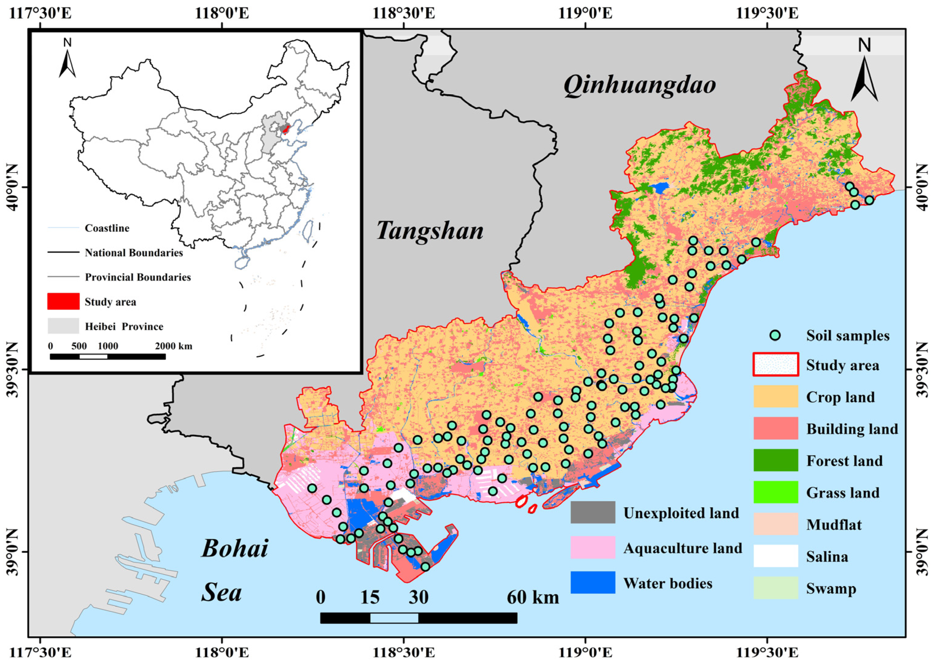
Figure 1. Location of the study area and soil samples.
Remotesensing 15 02907 g001
Figure 2. Schematic diagram of random forest method.
Remotesensing 15 02907 g002
Figure 3. Overview of the flowchart for STN content prediction.
Remotesensing 15 02907 g003
Figure 4. Scatter plot of predicted STN content values and the measured STN content values using RF, GBM, and XGBoost.
Remotesensing 15 02907 g004
Figure 5. The relative importance of variables used for the STN content prediction in Model Ⅶ based on RF, GBM, and XGBoost methods.
Remotesensing 15 02907 g005
Figure 6. Spatial distribution map of STN content obtained based on the RF, GBM, and XGBoost methods (Model VII: Landsat-8 + Sentinel-1 + Sentinel-2 predictors).
Remotesensing 15 02907 g006
Table 1. List of remote sensing images in this study.
SatelliteDateNumber of ImagesPixel Size (m)Width of Cloth (km)
Landsat-824 October 2020230 × 30185
31 October 20201
Sentinel-115 September 2020110 × 10250
20 September 20201
Sentinel-216 September 2020310 × 10 and 20 × 20290
Table 2. List of all remote sensing variables in the study for STN prediction.
SatelliteDefinitionAbbreviationFormula
Landsat-8Coastal bandL_B1
Blue bandL_B2
Green bandL_B3
Red bandL_B4
Near-infrared bandL_B5
Shortwave infrared-1 bandL_B6
Shortwave infrared-2 bandL_B7
Normalized difference vegetation indexL_NDVI(L_B5 − L_B4)/L_B5 + L_B4)
Ratio vegetation indexL_RVIL_B5/L_B4
Difference vegetation indexL_DVIL_B5 − L_B4
Bare soil indexL_BSI1 + L B 4 + L B 6 L B 5 + L B 2 L B 4 + L B 6 + L B 5 + L B 2
Normalized difference built-up indexL_NDBI ( L _ B 6 L _ B 5 ) / ( L _ B 6 + L _ B 5 )
Normalized difference water indexL_NDWI ( L _ B 3 L _ B 5 ) / ( L _ B 3 + L _ B 5 )
Sentinel 1VV-polarization of the backscatter coefficientsVV
VH-polarization of the backscatter coefficientsVH
Polarization combination 1VV+VH
Polarization combination 2VV-VH
Polarization combination 3VV/VH
Sentinel-2Blue bandS_B2
Green bandS_B3
Red bandS_B4
Vegetation red edge-1S_B5
Vegetation red edge-2S_B6
Vegetation red edge-3S_B7
Near-infrared bandS_B8
Narrow near-infrared bandS_B8A
Shortwave infrared-1 bandS_B11
Shortwave infrared-2 bandS_B12
Normalized difference vegetation indexS_NDVI ( S _ B 8 S _ B 4 ) / ( S _ B 8 + S _ B 4 )
Ratio vegetation indexS_RVI S _ B 8 / S _ B 4
Difference vegetation indexS_DVI S _ B 8 S _ B 4
Bare soil indexS_BSI1 + S _ B 4 + S _ B 11 S _ B 8 + S _ B 2 S _ B 4 + S _ B 11 + S _ B 8 + S _ B 2
Normalized difference built-up indexS_NDBI ( S _ B 11 S _ B 8 ) / ( S _ B 11 + S _ B 8 )
Normalized difference water indexS_NDWI ( S _ B 3 S _ B 8 ) / ( S _ B 3 + S _ B 8 )
Chlorophyll index of Red-edgeS_CIRE ( S _ B 7 S _ B 5 ) 1
Normalized difference Red-edge 1S_NDRE1 ( S _ B 6 S _ B 5 ) / ( S _ B 6 + S _ B 5 )
Normalized difference Red-edge 2S_NDRE2 ( S _ B 7 S _ B 5 ) / ( S _ B 7 + S _ B 5 )
Normalized difference vegetation index red-edge 1S_NDVIRE1 ( S _ B 8 S _ B 5 ) / ( S _ B 8 + S _ B 5 )
Normalized difference vegetation index red-edge 2S_NDVIRE2(S_B8-S_B6)/(S_B8+S_B6)
Normalized difference vegetation index red-edge 3S_NDVIRE3(S_B8-S_B7)/(S_B8+S_B7)
Table 3. Summary statistics of measured STN content at sample locations.
Minimum (g·kg−1)Maximum (g·kg−1)Mean (g·kg−1)Median (g·kg−1)SD (g·kg−1)CV %
STN0.0522.3960.7450.7640.44659.866
Table 4. Different combinations of variables used as inputs for STN content prediction.
No.ModelVariables
1Model ILandsat-8 predictors
2Model IISentinel-1 predictors
3Model IIISentinel-2 predictors
4Model ⅣLandsat-8 + Sentinel-1 predictors
5Model ⅤLandsat-8 + Sentinel-2 predictors
6Model ⅥSentinel-1 + Sentinel-2 predictors
7Model ⅦLandsat-8 + Sentinel-1 + Sentinel-2 predictors
Table 5. Performance results of RF, GBM, and XGBoost in predicting STN content based on different combinations of variables. The most accurate results are shown in bold.
Modeling TechniqueModelRMSE (g·kg−1)MAE (g·kg−1)R2
RFI0.1930.1340.446
II0.2160.1580.411
III0.1940.1400.409
0.1830.1270.459
0.1810.1250.463
0.1790.1300.457
0.1750.1230.475
GBMI0.2470.1760.410
II0.2770.2080.391
III0.2390.1770.394
0.2100.1540.479
0.2010.1400.496
0.2050.1460.488
0.1840.1300.533
XGBoostI0.1760.1310.498
II0.2260.1710.431
III0.1670.1250.524
0.1600.1210.545
0.1380.1010.593
0.1500.1070.564
0.1270.0920.627
Table 6. Descriptive statistics of predicted map of STN content.
MethodMinimum (g·kg−1)Maximum (g·kg−1)Mean (g·kg−1)SD (g·kg−1)
RF0.171.640.820.22
GBM01.870.840.26
XGBoost0.092.010.800.28
Disclaimer/Publisher’s Note: The statements, opinions and data contained in all publications are solely those of the individual author(s) and contributor(s) and not of MDPI and/or the editor(s). MDPI and/or the editor(s) disclaim responsibility for any injury to people or property resulting from any ideas, methods, instructions or products referred to in the content.