Article

Hyperspectral Remote Sensing Images Feature Extraction Based on Spectral Fractional Differentiation

1
School of Electronic Engineering, Xi’an University of Posts and Telecommunications, Xi’an 710121, China
2
School of Computer Science and Technology, Shandong Technology and Business University, Yantai 264005, China
3
School of Electronic Engineering, Xidian University, Xi’an 710071, China
*
Author to whom correspondence should be addressed.
Remote Sens. 2023, 15(11), 2879; https://doi.org/10.3390/rs15112879
Submission received: 25 April 2023 / Revised: 23 May 2023 / Accepted: 30 May 2023 / Published: 1 June 2023
(This article belongs to the Section Remote Sensing Image Processing)

Abstract

:
To extract effective features for the terrain classification of hyperspectral remote-sensing images (HRSIs), a spectral fractional-differentiation (SFD) feature of HRSIs is presented, and a criterion for selecting the fractional-differentiation order is also proposed based on maximizing data separability. The minimum distance (MD) classifier, support vector machine (SVM) classifier, K-nearest neighbor (K-NN) classifier, and logistic regression (LR) classifier are used to verify the effectiveness of the proposed SFD feature, respectively. The obtained SFD feature is sent to the full connected network (FCN) and 1-dimensionality convolutional neural network (1DCNN) for deep-feature extraction and classification, and the SFD-Spa feature cube containing spatial information is sent to the 3-dimensionality convolutional neural network (3DCNN) for deep-feature extraction and classification. The SFD-Spa feature after performing the principal component analysis (PCA) on spectral pixels is directly connected with the first principal component of the original data and sent to 3DCNNPCA and hybrid spectral net (HybridSN) models to extract deep features. Experiments on four real HRSIs using four traditional classifiers and five network models have shown that the extracted SFD feature can effectively improve the accuracy of terrain classification, and sending SFD feature to deep-learning environments can further improve the accuracy of terrain classification for HRSIs, especially in the case of small-size training samples.

1. Introduction

Hyperspectral remote-sensing images (HRSIs) contain abundant spatial and spectral information simultaneously. The spectral dimension reveals the spectral curve characteristics of each pixel, while the spatial dimension reveals the spatial characteristics of the ground surface, and the organic fusion of spatial and spectral information is realized by HRSIs [1,2,3]. However, HRSIs have the characteristics of information redundancy and high dimensionality that bring difficulties and challenges to feature extraction and terrain classification [4,5].
For the feature extraction of HRSIs, the dimensionality reduction methods are usually utilized to project the HRSIs’ spectral pixels to a low-dimensionality feature subspace [6,7]. Principal component analysis (PCA) and linear discriminant analysis (LDA) are representative approaches [8,9]. PCA calculates the covariance matrix of the original data, then, the eigenvectors corresponding to the first several largest eigenvalues of the covariance matrix are selected, and the original spectral pixels are projected to the orthogonal subspace supported by these eigenvectors to achieve the feature extraction and dimensionality reduction. LDA projects the original spectral pixels into a low-dimensional subspace, which has the largest between-class scatters and the smallest within-class scatters so that the data have the best separability in the subspace.
In addition to reducing the dimensionality of HRSIs by feature extraction, discriminant features that can enhance the spectral differences of different terrains can also be achieved by other data analysis methods. Bao et al. have demonstrated that the derivatives of the spectral feature of HRSIs can capture the salient features of different land-cover categories, and have shown that in the case of small samples or poor data quality, combining the spectral first-order differentiation rather than second-order differentiation with the original spectral pixel can avoid the curse of dimensionality and improve the recognition rate [10]. Ye et al. extracted the spectral first-order differentiation in HRSIs and then used locality preserving nonnegative matrix factorization (LPNMF) and locality Fisher discrimination analysis (LFDA) to reduce the dimensionality of the original spectral pixel and spectral derivative, respectively, and, finally, performed feature fusion, which can effectively improve the classification performance [11].
At present, fractional differentiation is usually used in spectral analysis to estimate the contents of some elements or ions in soil or vegetation and is rarely used in spectral classification [12]. Lao et al. calculated the fractional differentiation of the soil spectral pixel in visible near-infrared spectroscopy to estimate the soil contents of salt and soluble ions [13]. Hong et al. used fractional differentiation to estimate soil organic carbon (SOC), wherein the spectral parameters derived from different spectral indices based on spectral fractional differentiation are combined to obtain the best estimation accuracy of SOC [14].
In recent years, convolutional neural networks have achieved remarkable results in the terrain classification of HRSIs [15]. Hu et al. applied a 1-dimensionality convolutional neural network (1DCNN) to HRSIs, which only used spectral information without considering spatial information [16]. Zhang et al. used PCA to reduce the dimensionality of spectral pixels and then used a 2-dimensionality convolutional neural network (2DCNN) for feature extraction and classification, which considered the spatial information of HRSIs [17]. To achieve full use of both the spectral and spatial information of HRSIs, Chen et al. used PCA to reduce the dimensionality of spectral pixels and sent the dimensionality-reduced data into a 3-dimensionality convolutional neural network (3DCNN), and, simultaneously, extracted the spatial and spectral deep features of HRSIs [18].
This paper uses fractional differentiation to perform feature extraction on the pixel spectral curves of HRSIs from the aspect of data analysis, because fractional differentiation can retain part of the original characteristics of the data while obtaining the characteristics that express the differences in the data, and the order of the fractional differentiation can change with the different data. In this paper, a spectral fractional-differentiation (SFD) feature of HRSIs is presented, and a criterion for selecting the fractional-differentiation order is also proposed based on maximizing data separability. The minimum distance (MD) classifier, support vector machine (SVM) classifier, K-nearest neighbor (K-NN) classifier, and logistic regression (LR) classifier are used to verify the effectiveness of the proposed SFD feature, respectively. The obtained SFD feature is sent to the full connected network (FCN) [19] and 1DCNN for deep-feature extraction and classification, and the SFD-Spa feature cube containing spatial information is sent to 3DCNN for deep-feature extraction and classification. The SFD-Spa feature after performing PCA on spectral pixels is directly connected with the first principal component of the original data and sent to 3DCNNPCA and hybrid spectral net (HybridSN) [20] models to extract deep features. Compared with integer-order differentiation, the advantage of fractional-order differentiation is that it has memory and globality. When the order of the integer differentiation is just larger than that of fractional differentiation, fractional-order differentiation can preserve more low-frequency components of the signal, while the high- and middle-frequency components are also obviously enhanced [21]. The advantages of the presented HRSIs SFD feature are as follows:
(1)
The presented SFD feature preserves both the overall curve shape and local burrs characteristics of the pixel spectral curves of HRSIs, which is very suitable for terrain classification. The overall curve shapes of spectral curves correspond to the low-frequency components and the local burrs correspond to the high-frequency components of the pixel spectral curve. For HRSIs terrain classification, the shape characteristics of spectral curves contribute most to the discriminant of quite different terrains, such as water, soil, and plants; while the local burr characteristics contribute most to the identification of the different terrains which have similar spectral curves, such as wheat and soybean. These two characteristics are both important, however, the integer differentiation invariably enhanced the high-frequency components, i.e., local burrs while losing most of the low-frequency components, i.e., the shape characteristics of spectral curves. Fractional differentiation preserves the low-frequency components sufficiently while amplifying the high-frequency components remarkably, thus, the presented SFD feature contains both the overall curve shape and local burr characteristics of the spectral curves;
(2)
The order of the fractional differentiation of the presented SFD feature can be selected by achieving the best separability. With the increase in the differentiation order, the shape characteristics of the original spectral curve are less preserved, while the local burr characteristics are enhanced more significantly. In view of such character, a criterion for selecting the appropriate fractional-differentiation order is presented based on achieving the best data separability, which guarantees that the overall curve shape characteristics and the local burr characteristics are properly preserved in the resulting SFD feature, such that the quite different terrains and the similar terrains are all easy to identify.
Experimental results on four real HRSIs using four traditional classifiers and five network models have shown that the extracted SFD feature can effectively improve the terrain classification accuracy, and sending the SFD feature to deep-learning environments can further improve the terrain classification accuracy, especially in the case of small-size training samples [22,23].

2. Spectral Fractional-Differentiation (SFD) Feature

2.1. Fractional Differentiation

Among the many definitions of fractional differentiation, the commonly used three forms are Riemann–Liouville, Grümwald–Letnikvo, and Caputo [24]. In this paper, the Grümwald–Letnikvo definition is used to generalize the differentiation of continuous functions from integer order to fractional order, and the fractional-order differential expression is deduced by using the difference equation of integer-order differentiation.
According to the definition of integer-order differentiation, for a differentiable function f(x), its g-th integer-order differentiation is
f ( g ) ( x ) = lim h 0 1 h g j = 0 n ( 1 ) j ( g j ) f ( x j h )
where g , the binomial coefficient ( g j ) = Γ ( g + 1 ) Γ ( j + 1 ) Γ ( g j + 1 ) = g ! j ! ( g j ) ! , Γ ( · ) is Gamma function, Γ ( x ) = 0 e t t x 1 d t , and h represents the differential step size. Extending the order g to any real number v, the Grümwald–Letnikvo differentiation of f(x) is defined as
D x v a f ( x ) = lim h 0 1 h v j = 0 [ ( x a ) / h ] ( 1 ) j ( v j ) f ( x j h ) = lim h 0 1 h v j = 0 [ ( x a ) / h ] ( 1 ) j Γ ( v + 1 ) Γ ( j + 1 ) Γ ( v j + 1 ) f ( x j h )
where a represents the lower limit of f(x), and [(xa)/h] represents taking the integer part of (xa)/h [25].
Fractional differentiation defined in Equation (2) is a generalization of integer differentiation. When the order v is a positive integer, Equation (2) still holds, thus, the integer-order differentiation can be regarded as a special case of the fractional-order differentiation. Fractional differentiation is different from integer differentiation in numerical computing. During the calculation of the integer-order differentiation, the differential result of a point is only related to the information of the nearby points and unrelated to the information of other points; when the fractional differentiation is calculated, the differential result of a point is related to the information of all points before that point, and the points closer to it have greater weights in the calculation, thus, results in that fractional differentiation have memory and globality [25].

2.2. Spectral Fractional-Differentiation (SFD) Feature

The classical integer-order differentiation is a tool to describe the characteristics of the Euclidean space samples and is often utilized for signal extraction and singularity detection in signal analysis and processing. Fractional differentiation is a generalization of integer differentiation. Pu has pointed out that when the fractional-differentiation operation of a signal is performed, the high-frequency and middle-frequency components of the signal will be greatly improved, while the low-frequency components are retained nonlinearly [26]; and with the increase in the differentiation order, the improvement of the high-frequency and middle-frequency components will be enhanced, but fewer low-frequency components will be preserved [27]. In this paper, fractional differentiation is performed on the spectral pixel of HRSIs, and the resulting spectral fractional-differentiation (SFD) feature is used for terrain classification. Since the definition of Grümwald–Letnikvo fractional differentiation is generalized from the definition of integer differentiation and is expressed in discrete form, which is convenient for numerical calculation. Therefore, the presented SFD feature is defined according to the Grümwald–Letnikvo formula.
For a unary function f(x), let the differential step h = 1, then the expression of the v-th order fractional differentiation of f(x) is
f ( v ) ( x ) = f ( x ) + ( v ) f ( x 1 ) + ( v ) ( v + 1 ) 2 f ( x 2 ) + + Γ ( v + 1 ) n ! Γ ( v + t + 1 ) f ( x t )
which has (t + 1) terms.
For HRSIs, a spectral pixel can be regarded as a discrete form of a unary function. Assuming that each pixel has N spectral bands, for a spectral pixel x = [ x 0 , x 1 , x 2 , , x N 1 ] , the v-th order fractional-differentiation vector of x, i.e., the presented SFD feature, is
x ( v ) = [ a 0 x 1 + a 1 x 0 , a 0 x 2 + a 1 x 1 + a 2 x 0 , , a 0 x N 1 + a 1 x N 2 + a 2 x N 3 + + a N 1 x 0 ]
where a 0 , a 1 , , a N 1 are the first ( N 1 ) coefficients on the right side of Equation (3) and
{ a 0 = 1 a 1 = v a 2 = [ ( v ) ( v + 1 ) ] / 2 a 3 = [ ( v ) ( v + 1 ) ( v + 2 ) ] / 6 a N 1 = Γ ( v + 1 ) / [ ( N 1 ) ! Γ ( v + N ) ]
The dimensionality of the SFD feature x(v) is ( N 1 ) , and the components of x(v) correspond to the v-th order fractional differentiation of bands x 1 , x 2 , , x N 1 . In particular, when the order v equals 1, the expression of spectral fractional differentiation is the same as that of the first-order differentiation.

2.3. Criterion for Selecting Optimal Fractional-Differentiation Order

In the terrain classification of HRSIs based on the spectral pixel, when there only exist quite different terrains, such as water, soil, and plants, the overall curve shape characteristics of spectral curves, which correspond to the low-frequency components, contribute most to the discriminant. However, the phenomenon of different subjects with similar spectra commonly exists in HRSIs scenes [28,29]; in this case, the local burrs characteristics, which correspond to the high-frequency components, contribute most to the identification. In real HRSIs scenes, the phenomena of different objects with quite different spectra and different subjects with similar spectra both exist. This required that the feature extracted from the spectral curve should properly contain the low-frequency and high-frequency components simultaneously.
Shown in Figure 1 is the amplitude spectrum of the SFD feature of the corn-no-till class in the Indian Pines dataset, where the fractional-differentiation order v varies from 0 to 1.6 with step 0.4, the amplitude spectrum is taken logarithm for observation and the bases of the logarithm is 2. Figure 1 shows that as the fractional-differentiation order increases, the low-frequency components of the amplitude spectra decrease, while the mid-frequency and high-frequency components significantly increase. It can be concluded that the low-order SFD feature can enhance the high-frequency components while sufficiently retaining the low-frequency components of the spectral pixel, which is beneficial for preserving both the overall curve shape characteristics and the local burrs characteristics. However, how to select an appropriate differentiation order is a problem worth considering.
To study how the presented SFD feature is influenced by the fractional-differentiation order and to select the appropriate SFD order, the spectral curve of the corn-no-till class in the Indian Pines dataset is selected to extract the SFD feature with the fractional-differentiation order varies from 0 to 1.9 at step 0.1, thus, a total of 20 SFD curves are obtained, as shown in Figure 2.
It can be seen intuitively from Figure 2 that, as the differentiation order increases, the SFD values corresponding to the slowly changing parts of the original spectral curve gradually approach 0, and the SFD values corresponding to the local sharply changing parts dramatically increase. When the differentiation order increases from 0 to 1, the SFD curves still retain lots of shape characteristics of the original spectral curve, and the local sharp characteristics are enhanced. When the differentiation order increases from 1 to 1.9, the SFD curves lost most of the shape characteristics of the original spectral curve, and the local sharp characteristics are further enhanced. Therefore, for HRSIs terrain classification, when the differentiation order 0 < v < 1, the presented SFD feature contains the discriminant information benefit for classifying the different objects with quite different spectra and different subjects with similar spectra simultaneously and is very suitable for real HRSIs scenes. However, how to achieve more precise ranges of appropriate differentiation orders for different HRSIs is a problem worth further considering. In this paper, a criterion for selecting the SFD order is proposed based on maximizing the separability.
Assuming that the number of classes is C, let v denote the order of SFD, and the dimensionality of the SFD feature is ( N 1 ) , the within-class scatter matrix S w ( v ) and the between-class scatter matrix S b ( v ) in the ( N 1 ) -dimensionality SFD feature space are
S w ( v ) = i = 1 C P i 1 n i k = 1 n i ( x i k ( v ) m i ( v ) ) ( x i k ( v ) m i ( v ) ) T
and
S b ( v ) = i = 1 C P i ( m i ( v ) m ( v ) ) ( m i ( v ) m ( v ) ) T
, respectively, where ni represents the number of samples of class i, x i k ( v ) represents the v-th order fractional differentiation of the k-th sample of class i, Pi represents the prior probability of class i, m i ( v ) represents the mean of the v-th order fractional differentiations of class i, and m ( v ) = i = 1 C P i m i ( v ) represents the overall mean of the v-th order fractional differentiations.
The presented criterion for optimizing SFD order is
J ( v ) = T r ( S b ( v ) ) T r ( S w ( v ) ) ,
where “Tr()” represents the trace of a matrix. The principle of the SFD order selecting criterion is that the data separability should be maximized in the SFD feature space. T r ( S b ( v ) ) measures the variance of the class means in the v-th order SFD feature space, the larger T r ( S b ( v ) ) is, the greater the between-class separability is. T r ( S w ( v ) ) measures the within-class divergence in the v-th order SFD feature space, the smaller the T r ( S w ( v ) ) is, the smaller the within-class divergence is. Therefore, J(v) evaluates the data separability in the v-th order SFD feature space, by maximizing J, the data separability in the SFD feature space is maximized, thus, the optimal SFD order is
v * = arg max v J ( v ) .
Shown in Figure 3 are the variations of criterion J with the SFD order v on 4 real HRSIs datasets.
Figure 3 shows that, when the SFD order 0 < v < 1, Botswana, Indian Pines, and Salinas datasets have the same variation trend, they all have obvious peaks as 0.4 v 0.6 , as the SFD order v increases, the criterion J becomes smaller, which means smaller data separability, this is consistent with the analysis of Figure 1. For the Pavia University dataset, criterion J has an obvious peak as 0.5 v 0.7 and then decreases with the increase in v, and an inflection point occurs at v = 1.1, but the general trend is still the same as the other three datasets. Therefore, it is confirmed again that the SFD order v ranges between 0 and 1 is more conducive to improving the classification accuracy of HRSIs, and the precise appropriate SFD order range for each dataset is given.

3. Networks Structure and Parameter Settings

To further extract deep features, five network models are used for deep-feature extraction and terrain classification. The five network models used are fully connected network (FCN), one-dimensional convolutional neural network (1DCNN), three-dimensional convolutional neural network (3DCNN), three-dimensional convolutional neural network after spectral PCA dimensionality reduction (3DCNNPCA), and hybrid spectral net (HybridSN). Table 1 and Table 2 show the parameters and the number of output feature maps for each layer of the networks, respectively. N represents the dimension of the input dataset. C represents the number of classes. I, Conv, Po, and FC represent the input layer, convolutional layer, pooling layer, and fully connected layer, respectively. For example, Conv6 indicates that this layer is a convolutional layer located in the sixth layer of the network structure. ”√” means there exists an FC layer. <*> represents rounding up the calculation result.

4. Experimental Results

Firstly, using the proposed criterion J to select the appropriate SFD order for each dataset, the selected SFD order for Indian Pines, Botswana, Pavia University, and Salinas are 0.6, 0.3, 0.6, and 0.4, respectively. Additionally, then perform fractional differentiation on the pixel spectral curves with the selected order and achieve the SFD feature. Four traditional classifiers and five networks are used to verify the effectiveness of the resulting SFD feature. Among the five network models, the inputs of FCN and 1DCNN models are SFD feature vectors without spatial information, while the inputs of 3DCNN, 3DCNNPCA, and HybridSN contain spatial information. The input of 3DCNN is the SFD-Spa feature cube, and the input of 3DCNNPCA and HybridSN is the data cube by connecting the SFD-Spa feature after PCA with the first principal component of the original data. To unify the forms, the experimental results on five network models are all represented by “SFD”.

4.1. Experimental Datasets

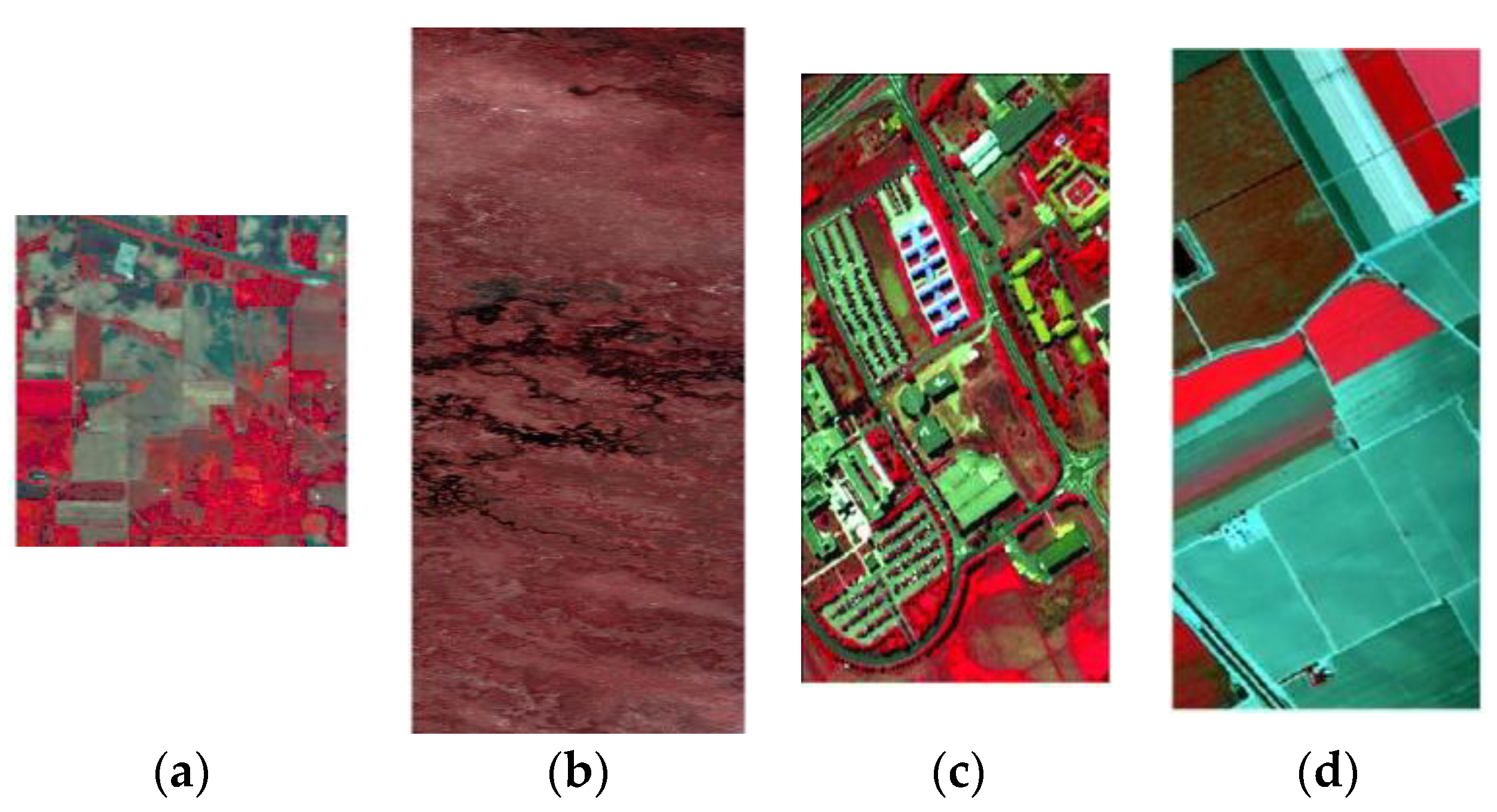
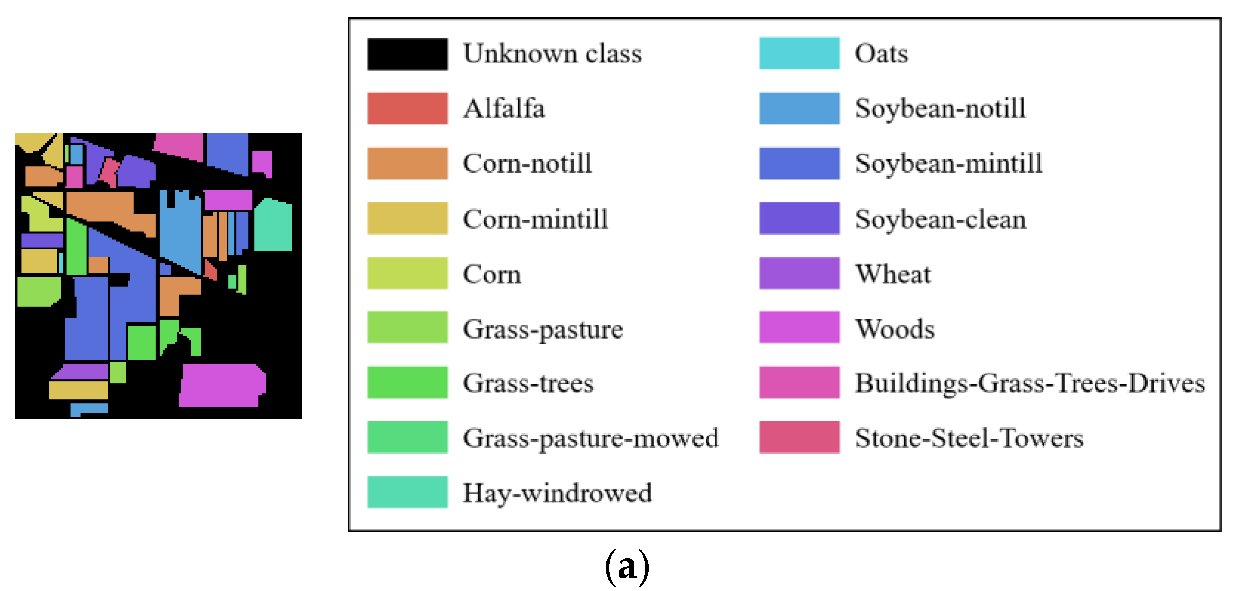
Four real HRSIs, namely, Indian Pines, Botswana, Pavia University, and Salinas, are used for the experiments. The Indian Pines dataset includes 16 classes, and the image size is 145 × 
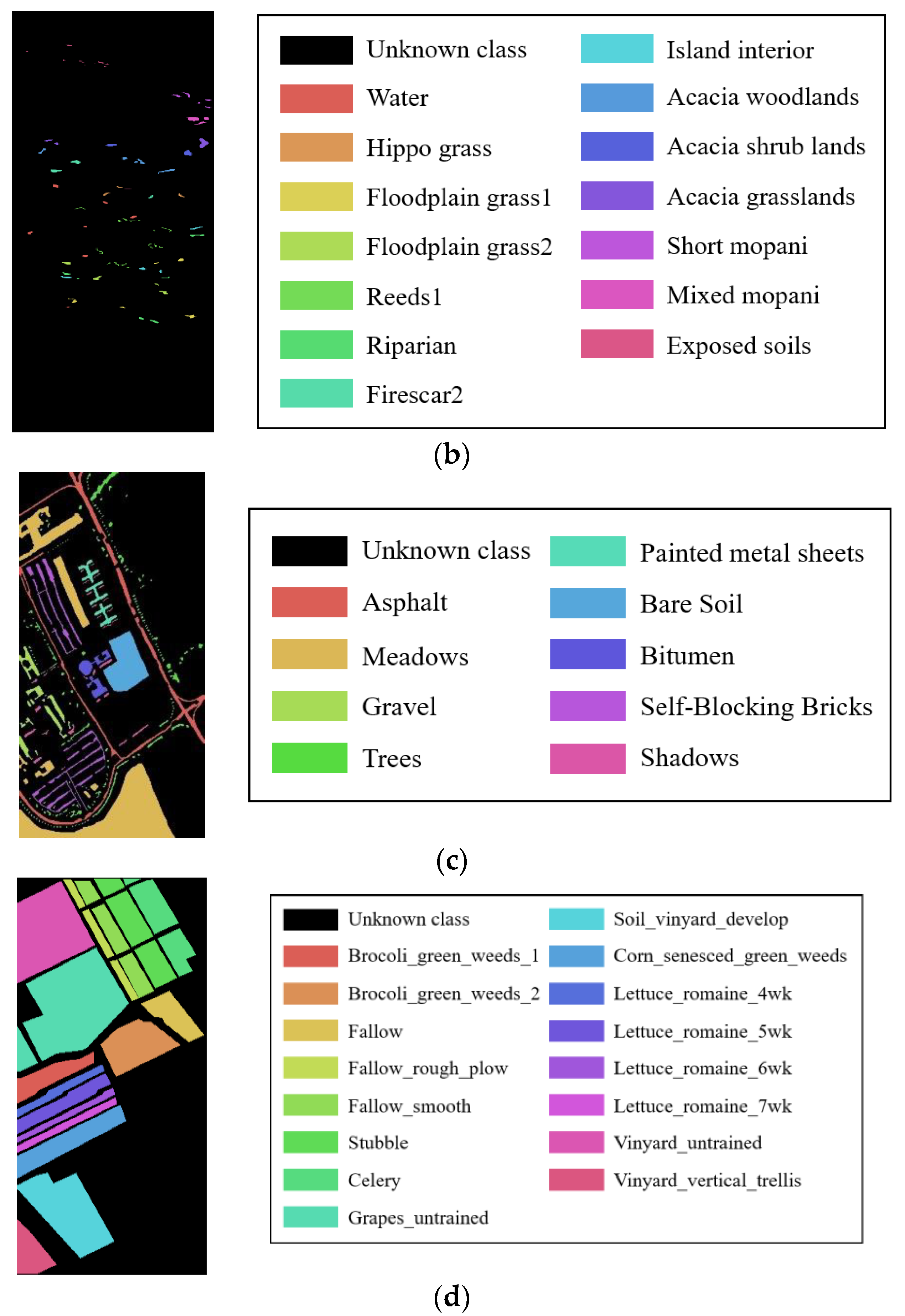
145, and a total of 10,249 pixels can be used to classify. After removing the bands 104–108, 150–163, and 220 affected by noise factors, 200 bands were finally left for the experiment. The Botswana dataset was obtained by NASA’s EO-1 satellite in the Botswana area. 14 terrain classes are included, and the image size is 1476 × 256, and 3248 of them are terrain pixels. After removing the bands affected by noise and water vapor, the bands 10–55, 82–97, 102–119, 134–164, and 187–220 were retained, i.e., a total of 145 bands were finally selected. Pavia University dataset contains 9 classes, the image size is 610 × 340, including 42,776 terrain pixels, and 103 bands were finally selected. The Salinas dataset has 16 classes, and the image size is 512 × 217. Bands 108–112, 154–167, and 220 were affected by noise and water vapor and were removed. 204 bands are reserved for research, and a total of 54,129 pixels can be used for terrain classification. Table 3 shows the specific sampling results of the experimental data. Figure 4 and Figure 5 show the false-color image and ground truth of these datasets.

4.2. Classification Results of Traditional Shallow Classifiers

The presented SFD feature will be compared with the spectral (Spe) feature, spectral first-order differential (Spe-1st) feature, and spectral second-order differential (Spe-2nd) feature. The above four features will be further compared through LDA dimensionality reduction to form SFDLDA, SpeLDA, Spe-1stLDA, and Spe-2ndLDA features. The comparison process will be validated using four traditional classifiers, namely, the MD classifier, the SVM classifier, the K-NN classifier, and the LR classifier. For each dataset, 20% of each class data are randomly selected as training samples and the rest as testing samples. Considering the randomness of the experiment, the average overall accuracy (AOA) and standard deviation (SD), average Kappa coefficient of 10 runs are used to describe the classification results. The experimental results on four real HRSIs datasets are shown in Table 4, Table 5, Table 6 and Table 7, “Average Kappa” is the abbreviation of “Average Kappa coefficient”, the optimal classification results are shown in bold in each column.
From Table 4, it can be seen that under 20% of the training samples in the Indian Pines dataset, compared to the original spectral feature Spe, the AOA of the extracted SFD features on SVM, MD, K-NN, and LR classifiers increased by 0.62%, 2.80%, 0.44%, and 6.59%, respectively; additionally, compared to the Spe-1st and Spe-2nd features, the AOA and average Kappa coefficient obtained by classification has significantly improved, indicating that the extracted SFD feature can achieve better accuracy in terrain classification. In addition, compared to the SpeLDA feature by performing LDA on the original spectral feature Spe, the SFDLDA feature has an AOA increase of 0.14%, 0.30%, 0.21%, and 0.12% on SVM, MD, K-NN, and LR classifiers; and compared to Spe-1stLDA feature and Spe-2ndLDA feature, the AOA and average Kappa coefficient have been improved to a certain extent, indicating that the extracted SFD feature can still retain their high separability after dimensionality reduction processing, enhancing the classification effect. In terms of the classification time, using the MD classifier as an example, the classification time for the Spe feature, Spe-1st feature, Spe-2nd feature, and SFD feature are 0.371 s, 0.361 s, 0.360 s, and 0.356 s, respectively. The result indicates that the extracted SFD feature can improve the accuracy of terrain classification while ensuring an almost constant classification rate.
Table 5 shows the classification results of the Botswana dataset under 20% of training samples. Compared to the original spectral feature Spe, the extracted SFD feature has significantly improved AOA and average Kappa coefficient on SVM, MD, K-NN, and LR classifiers compared to other features. Compared to the Spe feature, AOA has increased by 0.76%, 1.25%, 0.98%, and 2.48%, respectively, proving that the SFD feature can achieve better terrain classification accuracy. Meanwhile, compared to the SpeLDA feature, the AOA of the SFDLDA feature on SVM, MD, K-NN, and LR classifiers also increased by 0.10%, 0.16%, 0.11%, and 0.28%, respectively, indicating that the extracted SFD feature can still retain their high separability after dimensionality reduction processing, enhancing classification performance. In addition, the SD values of SFD and SFDLDA features are smaller than those of other features, further proving that the extracted features have a more stable classification effect. In terms of the classification time, using the MD classifier as an example, the classification time for the Spe feature, Spe-1st feature, Spe-2nd feature, and SFD feature are 0.132 s, 0.125 s, 0.136 s, and 0.126 s, respectively. The result indicates that the extracted SFD feature can effectively improve accuracy while maintaining runtime.
According to Table 6, it can be found that under 20% of training samples, the SFD feature extracted from the Pavia University dataset showed an increase in AOA on SVM, MD, K-NN, and LR classifiers by 1.47%, 2.80%, 0.69%, and 6.06%, respectively, compared to the original Spe feature. Moreover, compared to the Spe-1st and Spe-2nd features, the AOA and average Kappa coefficient of the SFD features were significantly improved, indicating that the extracted SFD feature can achieve better terrain classification accuracy. In addition, compared to the SpeLDA feature, the AOA of the SFDLDA feature on SVM, MD, K-NN, and LR classifiers increased by 0.87%, 6.02%, 1.09%, and 0.06%, respectively, and was also much greater than the AOA obtained from Spe-1stLDA and Spe-2ndLDA feature classification. Meanwhile, the SD values of the SFD feature and SFDLDA feature have decreased to varying degrees compared to most other features, indicating that the SFD feature has a certain degree of stability in terrain classification compared to other features. In terms of the classification time, using the MD classifier as an example, the classification time for the Spe feature, Spe-1st feature, Spe-2nd feature, and SFD feature are 0.748 s, 0.778 s, 0.721 s, and 0.755 s, respectively. The result indicates that the extracted SFD feature can improve the accuracy of terrain classification while ensuring an almost constant classification rate.
From Table 7, it can be observed that when selecting 20% of the training samples in the Salinas dataset, the extracted SFD feature showed an increase in AOA on SVM, MD, K-NN, and LR classifiers by 0.14%, 1.23%, 0.17%, and 2.41%, respectively, compared to the Spe feature. Moreover, the AOA was significantly improved compared to the Spe-1st feature and Spe-2nd feature. In addition, the AOA of the SFDLDA feature on SVM, MD, K-NN, and LR classifiers increased by 0.13%, 0.02%, 0.02%, and 0.03%, respectively, compared to the SpeLDA feature. The AOA and average Kappa coefficient obtained by the SFDLDA feature were also improved to some extent compared to the Spe-1stLDA feature and Spe-2ndLDA feature, indicating that the extracted SFD feature can still enhance the classification effect to some extent compared to other features. In addition, in terms of the classification time, using the MD classifier as an example, the classification time for the Spe feature, Spe-1st feature, Spe-2nd feature, and SFD feature are 1.680 s, 1.638 s, 1.666 s, and 1.642 s, respectively. The result indicates that the extracted SFD feature can effectively improve accuracy while maintaining runtime.

4.3. Classification Results of Networks

To extract deep features and verify the effectiveness of the SFD feature on different network structures, this paper sends the original spectral feature Spe, spectral first-order differential (Spe-1st) feature, spectral second-order differential (Spe-2nd) feature, spectral and frequency spectrum mixed feature (SFMF) [30], and extracted SFD feature into five different network structures for deep-feature extraction and classification, and compares the classification results. The experiments are conducted on a server with the RTX3080 graphical processing unit and 128 GB RAM, and the networks are implemented in Python. For each HRSIs dataset, 3%, 5%, and 10% samples of each class are randomly selected as training samples, and the rest are testing samples. Considering the randomness of the experimental results, the AOA and average Kappa coefficient of 10 runs were recorded to evaluate the classification effect. Table 8, Table 9, Table 10 and Table 11 show the experimental results on four real HRSIs datasets, where “Avg. Kap.” is the abbreviation of “Average Kappa coefficient”, the optimal classification results are shown in bold.
According to Table 8, it can be found that on the Indian Pines dataset, the AOA and average Kappa coefficient of the deep SFD feature are significantly higher than those of the deep Spe feature, deep Spe-1st feature, deep Spe-2nd feature, and SFMF on the five network models under 3%, 5%, and 10% training samples, and the deep Spe-1st and deep Spe-2nd features, generally, have lower AOA and average Kappa coefficient compared to the deep Spe feature. This indicates that the SFD feature extracted using fractional-order differentiation can enhance recognition performance compared to features extracted using first-order differentiation and second-order differentiation. In addition, when the proportion of training samples is small, the deep SFD feature performs relatively better in terrain classification accuracy compared to other features, such as the results of 3DCNNPCA and HybridSN models. Under the condition of 3% training samples, the number of training samples in each class is lower than 30 (except for classes 2, 11, and 14, the number of 3% samples per class is 42, 73, and 37, respectively), this indicates that even under the condition of small-size training samples, the SFD feature is superior to other features. Meanwhile, through comparison, it can be seen that the SD value of the deep SFD feature is also smaller compared to the deep Spe feature, indicating that the classification effect of the deep SFD feature has a better stability. In terms of running time, using the 3DCNNPCA model with 5% training samples as an example, the testing times for the Spe feature, Spe-1st feature, Spe-2nd feature, SFMF, and SFD feature are 0.475 s, 0.476 s, 0.475 s, 0.531 s, and 0.476 s, respectively. The result indicates that the extracted SFD feature can effectively improve accuracy while maintaining runtime.
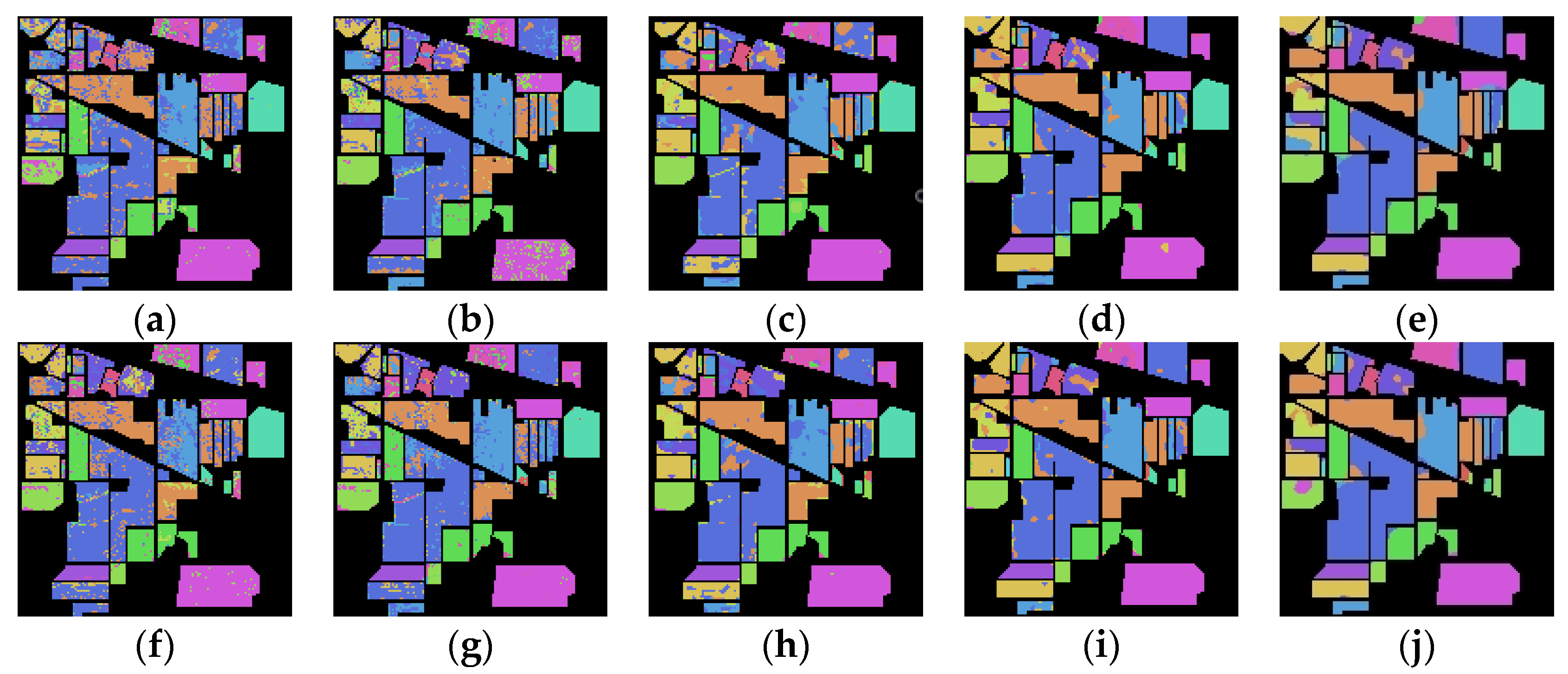
Figure 6 shows the classification maps of the Indian Pines dataset of deep Spe feature and deep SFD feature on five network models under 5% training samples. Through comparison, it can be found that the classification results of the deep SFD feature are, generally, better than those of the deep Spe feature on the five network models, with fewer misclassified pixels.
Table 9 shows the classification results of the presented SFD feature compared to the Spe feature, Spe-1st feature, Spe-2nd feature, and SFMF on five network models for the Botswana dataset with 3%, 5%, and 10% training samples. It can be found that the AOA of the SFD feature proposed in this paper has improved compared to the other three features on all five models, making it more effective for terrain classification. Additionally, when the proportion of training samples is smaller, the AOA and average Kappa coefficient of the SFD feature are significantly improved compared to other features. Under the condition of 3% training samples, the number of training samples in each class is far lower than 30, indicating that in the case of small-size training samples, the SFD feature can better exert its advantages compared to other features. At the same time, it can be found that the SD values of the SFD feature are, generally, smaller than those of other features, indicating that the SFD feature is more stable in the classification. In terms of running time, using the 3DCNNPCA model with 5% training samples as an example, the testing times for the Spe feature, Spe-1st feature, Spe-2nd feature, SFMF, and SFD feature are 0.349 s, 0.349 s, 0.348 s, 0.481 s, and 0.312 s, respectively. The result indicates that the extracted SFD feature not only improves the accuracy of terrain classification but also has a more efficient running rate compared to other features.
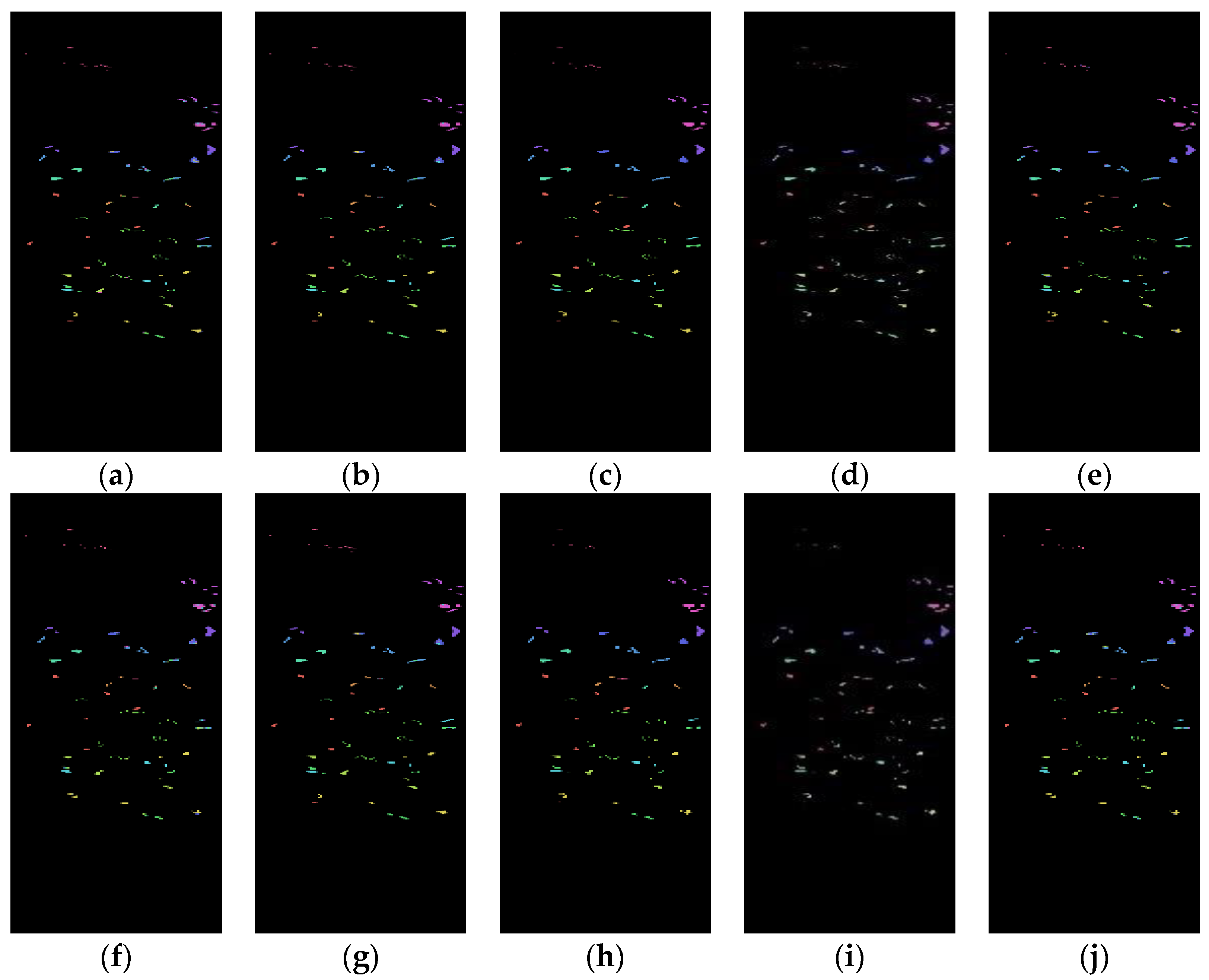
Figure 7 shows the classification results of the Spe and the presented SFD features of the Botswana dataset on five network models under 5% training samples. Through comparison, it can be seen that the classification results of the SFD feature are, generally, better than those of the Spe feature on the five network models, further demonstrating the effectiveness of the SFD feature in terrain classification.
From Table 10, it can be seen that on the Pavia University dataset, the presented SFD feature has higher AOA and average Kappa coefficient compared to the Spe feature, Spe-1st feature, Spe-2nd feature, and SFMF on the five network models at 3%, 5%, and 10% of the training samples. Additionally, the smaller the proportion of training samples, the more significant the improvement in the AOA of the SFD feature on certain models. For example, on 3DCNN, the AOA of the SFD feature increased by 2.98%, 0.95%, and 0.49% compared to Spe feature under 3%, 5%, and 10% training samples, respectively. Meanwhile, the SD values of the SFD feature are also smaller than those of other features, indicating that the presented SFD feature is more stable in the classification compared to other features. In terms of running time, using the 3DCNNPCA model with 5% training samples as an example, the testing times for the Spe feature, Spe-1st feature, Spe-2nd feature, SFMF, and SFD feature are 1.648 s, 1.646 s, 1.647 s, 2.068 s, and 1.634 s, respectively. The result indicates that the extracted SFD feature can effectively improve accuracy while maintaining runtime.
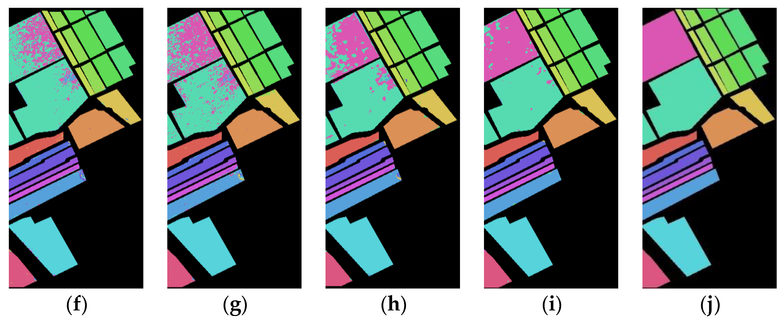
Figure 8 shows the classification maps of the Spe feature and the presented SFD feature on five network models for the Pavia University dataset under 5% training samples. Through comparison, it can be found that the classification results of the SFD feature are, generally, better than those of the Spe feature, which further proves the effectiveness of the extracted SFD feature in terrain classification.
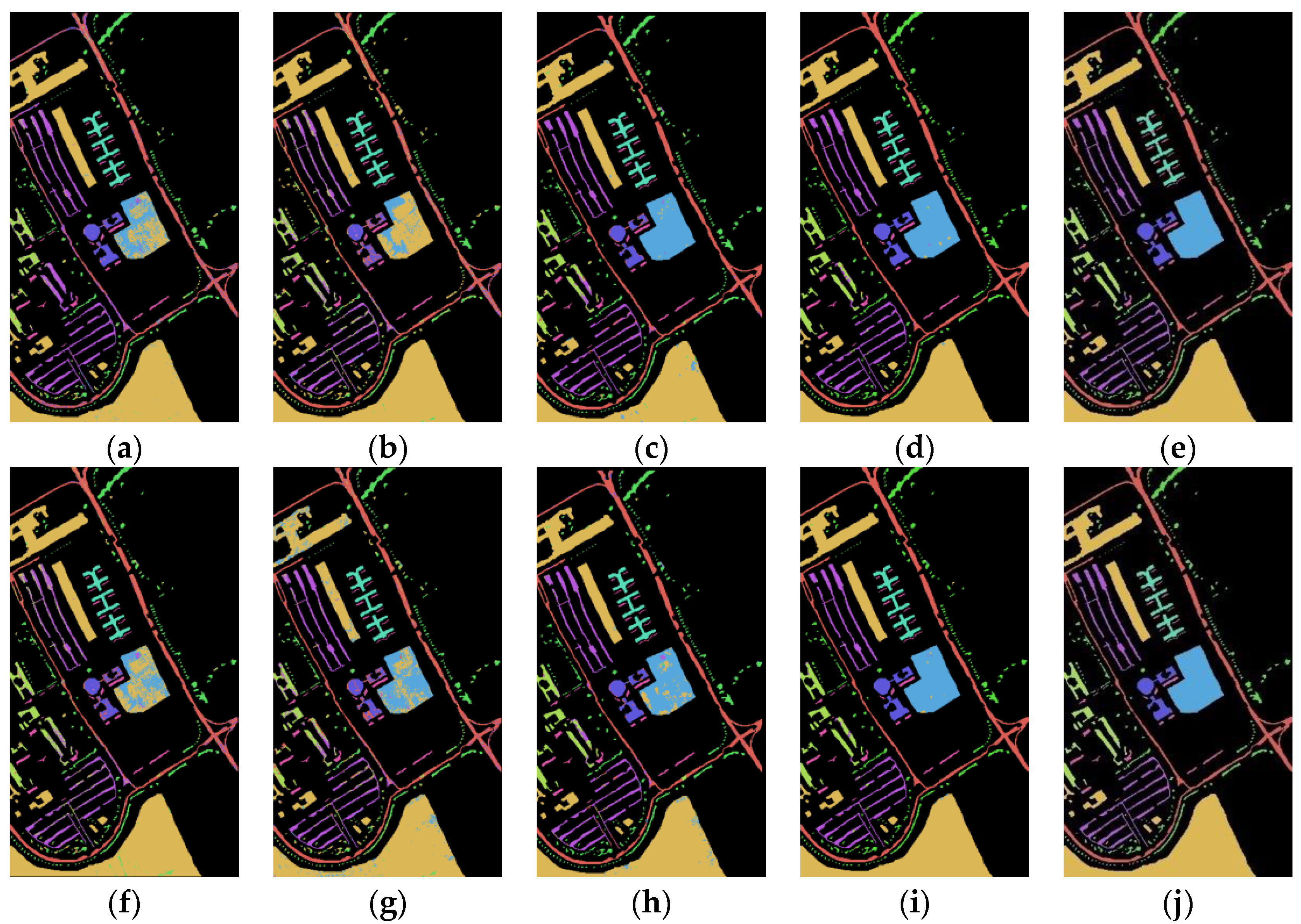
Figure 9 shows the classification maps of the Spe feature and SFD feature of the Salinas dataset on five network models under 5% training samples. It can be found that the classification results of the presented SFD feature are, generally, better than those of the Spe feature on five network models, and the misclassification rate of the SFD feature is lower compared to the Spe feature, indicating that the extracted SFD feature can effectively improve the classification accuracy.
From Table 11, it can be seen that at 3%, 5%, and 10% of the training samples, the SFD feature extracted from the Salinas dataset has a certain improvement in AOA and average Kappa coefficient compared to the Spe feature, Spe-1st feature, Spe-2nd feature, and SFMF on the five network models. Moreover, when the proportion of training samples is small, the AOA of the presented SFD feature is more significantly improved. For example, on the 3DCNN model, when the proportion of training samples is 3%, 5%, and 10%, the AOA of the SFD feature increased by 0.75%, 0.62%, and 0.25% compared to the Spe feature, respectively. In addition, the SD values of the SFD feature are, generally, smaller compared to other features, further indicating that the SFD feature has higher stability in the classification. In terms of running time, using the 3DCNNPCA model with 5% training samples as an example, the testing times for the Spe feature, Spe-1st feature, Spe-2nd feature, SFMF, and SFD feature are 2.021 s, 2.136 s, 2.056 s, 2.499 s, and 2.093 s, respectively. The result indicates that the extracted SFD feature can effectively improve accuracy while maintaining runtime.
Table 12 shows the small-size training samples experiments on the Pavia University and Salinas datasets under the condition of 30 training samples per class, the optimal classification results are shown in bold. From Table 12, it can be concluded that, in the case of small-size training samples, the SFD feature has greater advantages compared to other features on the Pavia University and Salinas datasets.

4.4. Discussion of Classification Results

From the above experimental results, it can be seen that the proposed SFD feature can effectively improve the classification accuracy of HRSIs. In the four HRSI datasets, the SFD feature has improved the accuracy of terrain classification to varying degrees. To demonstrate the effectiveness of the proposed criteria, Table 13 takes the MD classifier as an example and shows the AOA and SD vary with the SFD order v in the range of 0.1 to 0.9 at step 0.1 on four HRSIs datasets. For each dataset, 20% of each class data is randomly selected as a training sample and the rest are testing samples. The best result of each column is shown in bold.
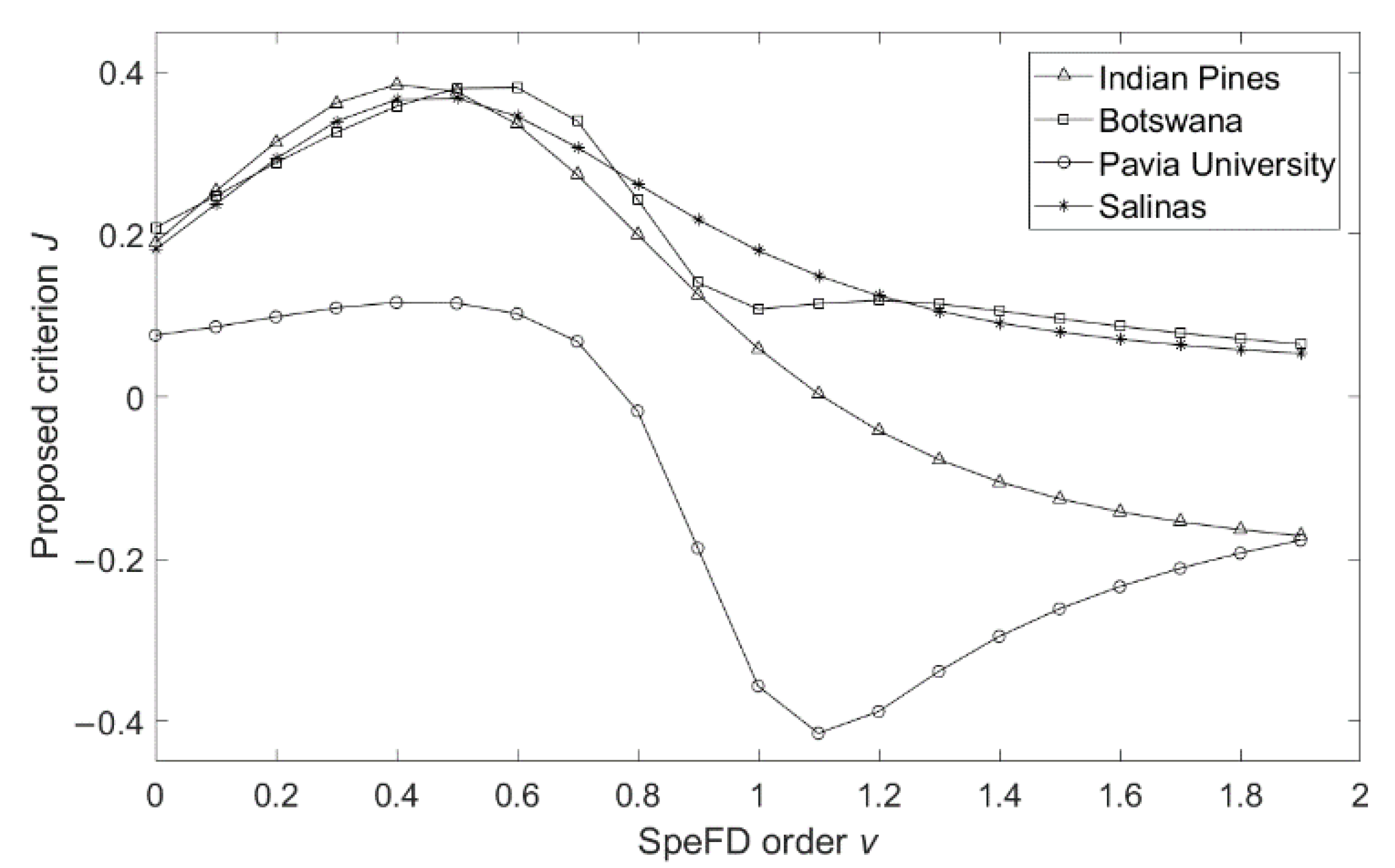
Table 13 shows that the SFD order v corresponding to the highest AOA of each dataset is mainly within the range of the peaks of criterion J in Figure 3. Additionally, the variation trend of classification accuracy with SFD order is also similar to that of criterion J with SFD order, which proves the feasibility of the presented SFD order selection criterion. It can be concluded that the presented criterion J is an effective method to select appropriate SFD order v, and performing fractional differentiation on the pixel spectral curves with the selected order v will achieve the efficient SFD feature that can improve the classification accuracy.
For two classes that are easily misclassified, the SFD feature shows its advantage and can enhance the separability between these two classes. Taking the Salinas dataset as an example, Table 14 shows the classification accuracy of each class and the overall accuracy, the significantly improved class at order 0.5 is shown in bold. It is shown in Table 14 that for most classes, the results of the SFD feature are better or equal to the original spectral feature. Because most classes in the Salinas dataset are vegetation and crops, which leads to different subjects with similar spectra, in this case, the local burrs characteristics of the pixel spectral curves, which correspond to the high-frequency components, contribute most to the identification. The extracted SFD feature can enhance the high-frequency components while sufficiently retaining the low-frequency components of the spectral pixel, thus, the separability of these similar classes will increase and the classification accuracy will be improved, which confirms the results discussed in Section 2.3.
The experimental results have verified the validity of the proposed SFD feature-extraction method. The reason behind the experimental phenomenon is that the presented SFD feature-extraction method uses fractional differentiation to extract both the low-frequency components characteristics and high-frequency components characteristics of the pixel spectral curves of HRSIs, which can preserve both the overall curve shape and local burrs characteristics of the pixel spectral curves of HRSIs. On the other hand, the experimental results also show the effectiveness of the presented criterion for selecting the fractional-differentiation order. The network models perform deep-feature extraction based on importing the SFD feature and, thus, achieve efficient deep features that can further improve terrain classification accuracy. Especially under the condition of small-size training samples, the terrain classification accuracy is improved more significantly.

5. Conclusions

In this paper, a spectral fractional-differentiation (SFD) feature of HRSIs is presented, and a fractional-differentiation order selection criterion is proposed. The MD classifier, SVM classifier, K-NN classifier, and LR classifier are used to evaluate the performance of the presented SFD feature. The obtained SFD feature is sent to the FCN and 1DCNN for deep-feature extraction and classification, and the SFD-Spa feature cube containing spatial information is sent to 3DCNN for deep-feature extraction and classification. The SFD-Spa feature after performing PCA on spectral pixels is directly connected with the first principal component of the original data and sent to 3DCNNPCA and HybridSN models to extract deep features. The experimental results on four real HRSIs show that the extracted SFD feature can effectively improve the accuracy of terrain classification, and sending SFD feature to deep-learning environments can further improve the accuracy of terrain classification for HRSIs, especially in the case of small-size training samples. The presented SFD feature-extraction method has limitations, such as the fact that the fractional-differentiation order needs to be selected, the SFD feature-extraction method cannot reduce the dimensionality of data, and the presented method should be performed on the datum one by one because there is no projection matrix that suits LDA or PCA.

Author Contributions

Conceptualization, Y.L. (Yang Li); formal analysis, Y.L. (Yang Li); funding acquisition, F.Z., Y.L. (Yi Liu), and J.L.; investigation, J.L. and Y.L. (Yang Li); methodology, J.L. and Y.L. (Yang Li); project administration, J.L., Y.L. (Yi Liu), and F.Z.; software, Y.L. (Yang Li); supervision, J.L.; validation, J.L.; visualization, Y.L. (Yang Li); writing—original draft, Y.L. (Yang Li); writing—review and editing, J.L. and Y.L. (Yi Liu). All authors have read and agreed to the published version of the manuscript.

Funding

This work was supported in part by the National Natural Science Foundation of China (no. 62176140, no. 62077038, and no. 61672405) and the Natural Science Foundation of Shaanxi Province of China (no. 2021JM-459).

Acknowledgments

The authors would like to thank the editors and anonymous reviewers who handled our paper.

Conflicts of Interest

The authors declare that there are no conflict of interest regarding the publication of this paper.

References

  1. Alcolea, A.; Paoletti, M.E.; Haut, J.M.; Resano, J.; Plaza, A. Inference in Supervised Spectral Classifiers for On-Board Hyperspectral Imaging: An Overview. Remote Sens. 2020, 12, 534. [Google Scholar] [CrossRef]
  2. Ma, W.; Yang, Q.; Wu, Y.; Zhao, W.; Zhang, X. Double-Branch Multi-Attention Mechanism Network for Hyperspectral Image Classification. Remote Sens. 2019, 11, 1307. [Google Scholar] [CrossRef]
  3. Li, S.; Song, W.; Fang, L.; Chen, Y.; Ghamisi, P.; Benediktsson, J.A. Deep Learning for Hyperspectral Image Classification: An Overview. IEEE Trans. Geosci. Remote Sens. 2019, 57, 6690–6709. [Google Scholar] [CrossRef]
  4. Mei, X.; Pan, E.; Ma, Y.; Dai, X.; Huang, J.; Fan, F.; Du, Q.; Zheng, H.; Ma, J. Spectral-Spatial Attention Networks for Hyperspectral Image Classification. Remote Sens. 2019, 11, 963. [Google Scholar] [CrossRef]
  5. Renard, N.; Bourennane, S.; Blanc-Talon, J. Denoising and Dimensionality Reduction Using Multilinear Tools for Hyperspectral Images. IEEE Geosci. Remote Sens. Lett. 2008, 5, 138–142. [Google Scholar] [CrossRef]
  6. Dong, Y.; Du, B.; Zhang, L.; Zhang, L. Dimensionality Reduction and Classification of Hyperspectral Images Using Ensemble Discriminative Local Metric Learning. IEEE Trans. Geosci. Remote Sens. 2017, 55, 2509–2524. [Google Scholar] [CrossRef]
  7. Li, N.; Zhou, D.; Shi, J.; Wu, T.; Gong, M. Spectral-Locational-Spatial Manifold Learning for Hyperspectral Images Dimensionality Reduction. Remote Sens. 2021, 13, 2752. [Google Scholar] [CrossRef]
  8. Licciardi, G.; Marpu, P.R.; Chanussot, J.; Benediktsson, J.A. Linear Versus Nonlinear PCA for the Classification of Hyperspectral Data Based on the Extended Morphological Profiles. IEEE Geosci. Remote Sens. Lett. 2012, 9, 447–451. [Google Scholar] [CrossRef]
  9. Bandos, T.V.; Bruzzone, L.; Camps-Valls, G. Classification of Hyperspectral Images with Regularized Linear Discriminant Analysis. IEEE Trans. Geosci. Remote Sens. 2009, 47, 862–873. [Google Scholar] [CrossRef]
  10. Bao, J.; Chi, M.; Benediktsson, J.A. Spectral Derivative Features for Classification of Hyperspectral Remote Sensing Images: Experimental Evaluation. IEEE J. Sel. Topics Appl. Earth Observ. Remote Sens. 2013, 6, 594–601. [Google Scholar] [CrossRef]
  11. Ye, Z.; He, M.; Fowler, J.E.; Du, Q. Hyperspectral Image Classification Based on Spectra Derivative Features and Locality Preserving Analysis. In Proceedings of the 2014 IEEE China Summit and International Conference on Signal and Information Processing, Xi’an, China, 4 September 2014; pp. 138–142. [Google Scholar]
  12. Tian, A.; Zhao, J.; Tang, B.; Zhu, D.; Fu, C.; Xiong, H. Hyperspectral Prediction of Soil Total Salt Content by Different Disturbance Degree under a Fractional-Order Differential Model with Differing Spectral Transformations. Remote Sens. 2021, 13, 4283. [Google Scholar] [CrossRef]
  13. Lao, C.; Chen, J.; Zhang, Z.; Chen, Y.; Ma, Y.; Chen, H.; Gu, X.; Ning, J.; Jin, J.; Li, X. Predicting the Contents of Soil Salt and Major Water-soluble Ions with Fractional-order Derivative Spectral Indices and Variable Selection. Comput. Electron. Agric. 2021, 182, 106031. [Google Scholar] [CrossRef]
  14. Hong, Y.; Guo, L.; Chen, S.; Linderman, M.; Mouazen, A.M.; Yu, L.; Chen, Y.; Liu, Y.; Liu, Y.; Chen, H.; et al. Exploring the Potential of Airborne Hyperspectral Image for Estimating Topsoil Organic Carbon: Effects of Fractional-order Derivative and Optimal Band Combination Algorithm. Geoderma 2020, 365, 114228. [Google Scholar] [CrossRef]
  15. Gao, Q.; Lim, S.; Jia, X. Hyperspectral Image Classification Using Convolutional Neural Networks and Multiple Feature Learning. Remote Sens. 2018, 10, 299. [Google Scholar] [CrossRef]
  16. Hu, W.; Huang, Y.; Wei, L.; Zhang, F.; Li, H. Deep Convolutional Neural Networks for Hyperspectral Image Classification. J. Sens. 2015, 2015, 258619. [Google Scholar] [CrossRef]
  17. Xu, Y.; Du, B.; Zhang, F.; Zhang, L. Hyperspectral Image Classification Via a Random Patches Network. ISPRS J. Photogramm. Remote Sens. 2018, 142, 344–357. [Google Scholar] [CrossRef]
  18. Chen, Y.; Jiang, H.; Li, C.; Jia, X.; Ghamisi, P. Deep Feature Extraction and Classification of Hyperspectral Images Based on Convolutional Neural Networks. IEEE Trans. Geosci. Remote Sens. 2016, 54, 6232–6251. [Google Scholar] [CrossRef]
  19. Audebert, N.; Le Saux, B.; Lefevre, S. Deep Learning for Classification of Hyperspectral Data: A Comparative Review. IEEE Geosci. Remote Sens. Mag. 2019, 7, 159–173. [Google Scholar] [CrossRef]
  20. Roy, S.K.; Krishna, G.; Dubey, S.R.; Chaudhuri, B.B. HybridSN: Exploring 3-D–2-D CNN Feature Hierarchy for Hyperspectral Image Classification. IEEE Geosci. Remote Sens. Lett. 2020, 17, 277–281. [Google Scholar] [CrossRef]
  21. Chen, W.; Jia, Z.; Yang, J.; Kasabov, N.K. Multispectral Image Enhancement Based on the Dark Channel Prior and Bilateral Fractional Differential Model. Remote Sens. 2022, 14, 233. [Google Scholar] [CrossRef]
  22. Dong, S.; Quan, Y.; Feng, W.; Dauphin, G.; Gao, L.; Xing, M. A Pixel Cluster CNN and Spectral-Spatial Fusion Algorithm for Hyperspectral Image Classification with Small-Size Training Samples. IEEE J. Sel. Topics Appl. Earth Observ. Remote Sens. 2021, 14, 4101–4114. [Google Scholar] [CrossRef]
  23. Aydemir, M.S.; Bilgin, G. Semisupervised Hyperspectral Image Classification Using Small Sample Sizes. IEEE Geosci. Remote Sens. Lett. 2017, 14, 621–625. [Google Scholar] [CrossRef]
  24. Sun, H.; Chang, A.; Zhang, Y.; Chen, W. A Review on Variable-order Fractional Differential Equations: Mathematical Foundations, Physical Models, Numerical Methods and Applications. Fract. Calc. Appl. Anal. 2019, 22, 27–59. [Google Scholar] [CrossRef]
  25. Podlubny, I. Fractional Differential Equations; Academic Press: San Diego, CA, USA, 1999; pp. 43–48, 203. [Google Scholar]
  26. Pu, Y. Fractional Calculus Approach to Texture of Digital Image. In Proceedings of the 8th International Conference on Signal Processing, Guilin, China, 16 November 2006; pp. 1002–1006. [Google Scholar]
  27. Pu, Y.; Yuan, X.; Liao, K.; Chen, Z.; Zhou, J. Five Numerical Algorithms of Fractional Calculus Applied in Modern Signal Analyzing and Processing. J. Sichuan Univ. Eng. Sci. Ed. 2005, 37, 118–124. [Google Scholar]
  28. Fauvel, M.; Tarabalka, Y.; Benediktsson, J.A.; Chanussot, J.; Tilton, J.C. Advances in Spectral-spatial Classification of Hyperspectral Images. Proc. IEEE 2013, 101, 652–675. [Google Scholar] [CrossRef]
  29. Vali, A.; Comai, S.; Matteucci, M. Deep Learning for Land Use and Land Cover Classification Based on Hyperspectral and Multispectral Earth Observation Data: A Review. Remote Sens. 2020, 12, 2495. [Google Scholar] [CrossRef]
  30. Liu, J.; Yang, Z.; Liu, Y.; Mu, C. Hyperspectral Remote Sensing Images Deep Feature Extraction Based on Mixed Feature and Convolutional Neural Networks. Remote Sens. 2021, 13, 2599. [Google Scholar] [CrossRef]
Disclaimer/Publisher’s Note: The statements, opinions, and data contained in all publications are solely those of the individual author(s) and contributor(s), and not of MDPI and/or the editor(s). MDPI and/or the editor(s) disclaim responsibility for any injury to people or property resulting from any ideas, methods, instructions, or products referred to in the content.
Figure 1. Amplitude spectra of SFDs with different fractional-differentiation orders.
Remotesensing 15 02879 g001
Figure 2. SFD curves of corn-no-till with fractional-differentiation order varying from 0 to 1.9: (a) v = 0~0.4; (b) v = 0.5~0.9; (c) v = 1~1.4; (d) v = 1.5~1.9.
Remotesensing 15 02879 g002
Figure 3. Comparison of variations of J with SFD order v.
Remotesensing 15 02879 g003
Figure 4. The false-color image of four HRSIs datasets: (a) Indian Pines; (b) Botswana; (c) Pavia University; (d) Salinas.
Remotesensing 15 02879 g004
Figure 5. The ground truth of four HRSIs datasets: (a) Indian Pines; (b) Botswana; (c) Pavia University; (d) Salinas.
Remotesensing 15 02879 g005aRemotesensing 15 02879 g005b
Figure 6. Indian Pines dataset classification map: (a) Spe feature in FCN model with 69.36% AOA; (b) Spe feature in 1DCNN model with 77.12% AOA; (c) Spe feature in 3DCNN model with 81.53% AOA; (d) Spe feature in 3DCNNPCA model with 90.77% AOA; (e) Spe feature in HybridSN model with 93.81% AOA; (f) SFD feature in FCN model with 73.88% AOA; (g) SFD feature in 1DCNN model with 79.77% AOA; (h) SFD feature in 3DCNN model with 85.39% AOA; (i) SFD feature in 3DCNNPCA model with 91.44% AOA; (j) SFD feature in HybridSN model with 95.47% AOA.
Remotesensing 15 02879 g006
Figure 7. Botswana dataset classification map: (a) Spe feature in FCN model with 82.48% AOA; (b) Spe feature in 1DCNN model with 82.76% AOA; (c) Spe feature in 3DCNN model with 89.02% AOA; (d) Spe feature in 3DCNNPCA model with 98.57% AOA; (e) Spe feature in HybridSN model with 96.45% AOA; (f) SFD feature in FCN model with 87.37% AOA; (g) SFD feature in 1DCNN model with 84.58% AOA; (h) SFD feature in 3DCNN model with 91.92% AOA; (i) SFD feature in 3DCNNPCA model with 99.16% AOA; (j) SFD feature in HybridSN model with 97.93% AOA.
Remotesensing 15 02879 g007
Figure 8. Pavia University dataset classification map: (a) Spe feature in FCN model with 85.36% AOA; (b) Spe feature in 1DCNN model with 81.66% AOA; (c) Spe feature in 3DCNN model with 93.03% AOA; (d) Spe feature in 3DCNNPCA model with 98.89% AOA; (e) Spe feature in HybridSN model with 99.29% AOA; (f) SFD feature in FCN model with 87.73% AOA; (g) SFD feature in 1DCNN model with 83.39% AOA; (h) SFD feature in 3DCNN model with 94.34% AOA; (i) SFD feature in 3DCNNPCA model with 99.12% AOA; (j) SFD feature in HybridSN model with 99.79% AOA.
Remotesensing 15 02879 g008
Figure 9. Salinas dataset classification map: (a) Spe feature in FCN model with 88.77% AOA; (b) Spe feature in 1DCNN model with 87.14% AOA; (c) Spe feature in 3DCNN model with 91.02% AOA; (d) Spe feature in 3DCNNPCA model with 97.89% AOA; (e) Spe feature in HybridSN model with 99.78% AOA; (f) SFD feature in FCN model with 90.95% AOA; (g) SFD feature in 1DCNN model with 89.35% AOA; (h) SFD feature in 3DCNN model with 92.98% AOA; (i) SFD feature in 3DCNNPCA model with 98.86% AOA; (j) SFD feature in HybridSN model with 99.94% AOA.
Remotesensing 15 02879 g009aRemotesensing 15 02879 g009b
Table 1. Parameter settings for five network models.
FCN1DCNN3DCNN3DCNNPCAHybridSN
I11 × N1 × N1 × N11 × 11 × N25 × 25 × N
Conv2-<1 × N/9>7 × 7 × 33 × 3 × 73 × 3 × 7
Po3-1 × <<N/9>/5>---
Conv4--3 × 3 × 33 × 3 × 53 × 3 × 5
Po5-----
Conv6---3 × 3 × 33 × 3 × 3
Po7-----
Conv8---3 × 3 × 33 × 3
Po9-----
FC1
FC2-
FC3--
FC4----
Table 2. Number of output feature maps for five network models.
FCN1DCNN3DCNN3DCNNPCAHybridSN
I111111
Conv2-20288
Po3-20---
Conv4--41616
Po5-----
Conv6---3232
Po7-----
Conv8---6464
Po9-----
FC12048100C256256
FC24096C-128128
FC32048--CC
FC4C----
Table 3. Category number, name, and sample number of each dataset.
Category NumberCategory
Name
Sample NumberCategory NumberCategory
Name
Sample Number
Indian Pines
1Alfalfa469Oats20
2Corn-notill142810Soybean-notill972
3Corn-mintill83011Soybean-mintill2455
4Corn23712Soybean-clean593
5Grass-pasture48313Wheat205
6Grass-trees73014Woods1265
7Grass-pasture-mowed2815Building-Grass-Trees-Drives386
8Hay-windrowed47816Stone-Steel-Towers93
Botswana
1Water2708Island interior203
2Hippo grass1019Acacia woodlands314
3Floodplain grass125110Acacia shrub lands248
4Floodplain grass221511Acacia grasslands305
5Reeds126912Short mopani181
6Riparian26913Mixed mopani268
7Firescar225914Exposed soils95
Pavia University
1Asphalt66316Bare Soil5029
2Meadows18,6497Bitumen1330
3Gravel20998Self-Blocking Bricks3682
4Tress30649Shadows947
5Painted metal sheets1345
Salinas
1Brocoli_green_weeds_120099Soil_vinyard_develop6203
2Brocoli_green_weeds_2372610Corn_senesced_green_weeds3278
3Fallow197611Lettuce_romaine_4wk1068
4Fallow_rough_plow139412Lettuce_romaine_5wk1927
5Fallow_smooth267813Lettuce_romaine_6wk916
6Stubble395914Lettuce_romaine_7wk1070
7Celery357915Vinyard_untrained7268
8Grapes_untrained11,27116Vinyard_vertical_trellis1807
Table 4. Classification results of the Indian Pines dataset on traditional shallow classifiers.
ClassifierSVMMDK-NNLR
AOA (%) ± SD (%) Average KappaAOA (%) ± SD (%) Average KappaAOA (%) ± SD (%) Average KappaAOA (%) ± SD (%) Average Kappa
Spe82.93 ± 0.360.80546.15 ± 0.890.40477.93 ± 0.440.74856.30 ± 0.790.476
Spe-1st67.54 ± 0.610.62246.02 ± 0.800.40250.41 ± 0.510.43159.62 ± 1.330.523
Spe-2nd54.83 ± 0.340.46839.50 ± 0.850.33239.67 ± 0.370.31051.83 ± 0.670.428
SFD83.55 ± 0.380.81248.95 ± 0.710.43378.37 ± 0.540.75362.89 ± 1.350.562
SpeLDA79.53 ± 0.410.76573.70 ± 0.460.70478.75 ± 0.800.75673.82 ± 0.520.699
Spe-1stLDA79.39 ± 0.400.76473.39 ± 0.650.70078.12 ± 0.690.74973.84 ± 0.600.700
Spe-2ndLDA79.26 ± 0.460.76272.97 ± 0.500.69677.67 ± 0.680.74473.33 ± 0.290.694
SFDLDA79.67 ± 0.430.76774.00 ± 0.510.70778.96 ± 0.870.75973.94 ± 0.410.701
Table 5. Classification results of the Botswana dataset on traditional shallow classifiers.
ClassifierSVMMDK-NNLR
AOA (%) ± SD (%) Average KappaAOA (%) ± SD (%) Average KappaAOA (%) ± SD (%) Average KappaAOA (%) ± SD (%) Average Kappa
Spe91.79 ± 0.540.91180.76 ± 0.680.79390.71 ± 0.380.89987.09 ± 1.200.860
Spe-1st87.22 ± 0.810.86279.69 ± 0.840.78078.26 ± 1.080.76586.13 ± 0.850.850
Spe-2nd74.77 ± 1.130.72665.74 ± 1.170.62955.03 ± 0.740.51571.96 ± 1.170.696
SFD92.55 ± 0.540.91982.01 ± 0.530.80591.69 ± 0.370.91089.57 ± 0.920.887
SpeLDA93.65 ± 0.450.93192.85 ± 0.460.92393.40 ± 0.530.92989.09 ± 0.870.882
Spe-1stLDA93.22 ± 0.520.92792.43 ± 0.580.91892.87 ± 0.530.92387.23 ± 0.570.862
Spe-2ndLDA92.42 ± 0.730.91891.69 ± 0.500.91092.05 ± 0.560.91485.44 ± 0.940.842
SFDLDA93.75 ± 0.440.94493.01 ± 0.430.92493.51 ± 0.460.93089.37 ± 0.660.885
Table 6. Classification results of the Pavia University dataset on traditional shallow classifiers.
ClassifierSVMMDK-NNLR
AOA (%) ± SD (%) Average KappaAOA (%) ± SD (%) Average KappaAOA (%) ± SD (%) Average KappaAOA (%) ± SD (%) Average Kappa
Spe89.96 ± 0.170.86559.54 ± 0.440.50184.77 ± 0.250.79576.82 ± 1.370.681
Spe-1st86.07 ± 0.140.81158.66 ± 0.830.49268.43 ± 0.210.57481.53 ± 0.230.748
Spe-2nd74.42 ± 0.180.64330.82 ± 1.370.23045.48 ± 0.260.24474.62 ± 0.230.651
SFD91.43 ± 0.100.88562.34 ± 0.350.54485.46 ± 0.230.80482.88 ± 0.500.767
SpeLDA88.62 ± 0.300.84871.50 ± 0.340.64387.16 ± 0.410.82781.91 ± 0.390.754
Spe-1stLDA88.71 ± 0.280.84976.54 ± 0.370.69987.54 ± 0.200.83280.14 ± 0.180.729
Spe-2ndLDA87.05 ± 0.110.82773.88 ± 0.470.66985.58 ± 0.170.80679.29 ± 0.150.718
SFDLDA89.49 ± 0.290.85977.52 ± 0.320.71188.25 ± 0.210.84281.97 ± 0.390.755
Table 7. Classification results of the Salinas dataset on traditional shallow classifiers.
ClassifierSVMMDK-NNLR
AOA (%) ± SD (%) Average KappaAOA (%) ± SD (%) Average KappaAOA (%) ± SD (%) Average KappaAOA (%) ± SD (%) Average Kappa
Spe93.62 ± 0.090.92975.57 ± 0.270.72990.53 ± 0.160.89584.51 ± 0.910.826
Spe-1st91.39 ± 0.060.90475.42 ± 0.140.72786.68 ± 0.160.85286.80 ± 0.920.852
Spe-2nd88.16 ± 0.110.86873.29 ± 0.190.70481.71 ± 0.150.79681.96 ± 0.580.797
SFD93.76 ± 0.100.93076.80 ± 0.310.74390.70 ± 0.170.89686.92 ± 0.770.853
SpeLDA94.26 ± 0.080.93691.33 ± 0.090.90393.57 ± 0.090.92891.21 ± 0.080.902
Spe-1stLDA94.37 ± 0.090.93891.34 ± 0.100.90493.58 ± 0.100.92891.22 ± 0.100.902
Spe-2ndLDA94.30 ± 0.080.93791.33 ± 0.100.90393.57 ± 0.080.92891.22 ± 0.090.902
SFDLDA94.39 ± 0.080.93891.35 ± 0.090.90493.59 ± 0.100.92891.24 ± 0.080.902
Table 8. Classification results of the Indian Pines dataset on network models.
ModelFCN1DCNN3DCNN3DCNNPCAHybridSN
AOA (%) ± SD (%) Avg. Kap.AOA (%) ± SD (%) Avg. Kap.AOA (%) ± SD (%) Avg. Kap.AOA (%) ± SD (%) Avg. Kap.AOA (%) ± SD (%) Avg. Kap.
3% training samples
Spe62.15 ± 1.420.56164.17 ± 1.130.58574.12 ± 4.730.70584.61 ± 0.900.82387.57 ± 1.040.858
Spe-1st53.83 ± 2.190.46761.52 ± 1.460.55576.68 ± 2.640.73384.15 ± 0.490.81988.77 ± 0.550.871
Spe-2nd49.61 ± 1.360.41549.33 ± 1.490.41570.16 ± 2.410.65682.86 ± 0.800.80488.64 ± 0.710.870
SFMF61.44 ± 0.920.55568.47 ± 2.050.63773.20 ± 2.280.69384.90 ± 0.640.82587.98 ± 0.860.863
SFD64.58 ± 1.940.58973.10 ± 1.560.69177.61 ± 3.610.74385.74 ± 0.680.83388.95 ± 0.930.874
5% training samples
Spe67.62 ± 2.650.62776.00 ± 1.270.72479.41 ± 4.350.76590.98 ± 0.490.89593.20 ± 1.560.922
Spe-1st59.53 ± 0.370.53165.23 ± 1.120.60181.89 ± 1.460.79489.37 ± 1.050.87994.61 ± 0.820.938
Spe-2nd52.25 ± 1.430.44951.61 ± 0.780.44476.49 ± 1.120.73189.59 ± 0.470.88194.42 ± 0.470.936
SFMF68.28 ± 1.450.63474.24 ± 1.300.70582.72 ± 1.900.80390.86 ± 0.510.89493.86 ± 0.930.927
SFD72.85 ± 1.880.68778.79 ± 1.160.75383.41 ± 2.590.81191.24 ± 0.270.89894.99 ± 0.510.935
10% training samples
Spe73.80 ± 3.950.70076.70 ± 1.430.73387.75 ± 2.320.86195.43 ± 0.550.94398.04 ± 0.260.978
Spe-1st63.61 ± 0.650.58169.54 ± 0.980.65087.46 ± 1.510.85793.31 ± 0.470.92498.15 ± 0.290.979
Spe-2nd55.45 ± 0.520.48753.33 ± 0.800.46481.79 ± 1.180.79292.41 ± 0.460.91398.10 ± 0.190.978
SFMF74.52 ± 1.350.70879.09 ± 0.730.76188.70 ± 1.450.87195.72 ± 0.510.94698.33 ± 0.210.980
SFD77.95 ± 3.190.74981.64 ± 0.920.79089.05 ± 1.650.86996.03 ± 0.370.95098.46 ± 0.190.982
Table 9. Classification results of the Botswana dataset on network models.
ModelFCN1DCNN3DCNN3DCNNPCAHybridSN
AOA (%) ± SD (%) Avg. Kap.AOA (%) ± SD (%) Avg. Kap.AOA (%) ± SD (%) Avg. Kap.AOA (%) ± SD (%) Avg. Kap.AOA (%) ± SD (%) Avg. Kap.
3% training samples
Spe81.19 ± 1.410.79676.26 ± 2.280.74387.32 ± 4.780.86397.14 ± 0.790.96993.23 ± 1.750.927
Spe-1st74.09 ± 2.330.71955.74 ± 3.550.51581.42 ± 6.270.79997.35 ± 0.730.97193.60 ± 2.030.931
Spe-2nd59.89 ± 2.320.56549.14 ± 2.700.44477.73 ± 2.790.75995.91 ± 0.670.95691.73 ± 1.340.910
SFMF82.03 ± 1.800.80571.38 ± 1.550.68988.47 ± 0.970.87597.88 ± 0.820.97493.87 ± 1.420.932
SFD86.44 ± 1.360.85378.13 ± 1.870.76390.24 ± 2.280.89498.36 ± 0.310.98194.33 ± 1.130.939
5% training samples
Spe81.36 ± 2.370.78681.78 ± 1.970.80390.14 ± 4.130.89398.70 ± 0.650.98497.05 ± 1.060.968
Spe-1st77.82 ± 2.100.75979.63 ± 0.890.77989.98 ± 1.610.89197.45 ± 1.160.97297.28 ± 1.020.971
Spe-2nd65.30 ± 1.680.62456.41 ± 2.820.52486.26 ± 1.320.85196.03 ± 0.980.95795.61 ± 1.270.953
SFMF83.22 ± 2.610.81879.38 ± 1.920.77690.16 ± 2.540.89398.52 ± 0.750.98196.41 ± 1.720.965
SFD87.02 ± 0.670.85983.59 ± 1.130.82291.03 ± 1.200.90399.02 ± 0.150.98797.49 ± 0.450.973
10% training samples
Spe86.42 ± 0.830.85386.13 ± 0.730.85093.69 ± 2.800.93299.09 ± 0.350.99099.40 ± 0.580.994
Spe-1st83.83 ± 0.800.82586.55 ± 1.040.85493.59 ± 2.810.93199.01 ± 0.330.98999.50 ± 0.250.995
Spe-2nd73.86 ± 2.080.71776.91 ± 1.460.75092.42 ± 1.280.91898.68 ± 0.220.98699.18 ± 0.550.991
SFMF88.08 ± 1.020.87186.89 ± 1.160.85894.37 ± 1.910.93999.12 ± 0.280.99199.51 ± 0.380.995
SFD89.94 ± 1.000.89187.00 ± 0.760.85995.24 ± 1.100.94899.44 ± 0.110.99399.61 ± 0.280.996
Table 10. Classification results of the Pavia University dataset on network models.
ModelFCN1DCNN3DCNN3DCNNPCAHybridSN
AOA (%) ± SD (%) Avg. Kap.AOA (%) ± SD (%) Avg. Kap.AOA (%) ± SD (%) Avg. Kap.AOA (%) ± SD (%) Avg. Kap.AOA (%) ± SD (%) Avg. Kap.
3% training samples
Spe84.55 ± 1.580.79479.13 ± 0.620.71388.51 ± 5.470.84898.17 ± 0.230.97598.47 ± 0.620.980
Spe-1st79.62 ± 1.270.72772.51 ± 1.870.62688.79 ± 1.890.85398.14 ± 0.360.97599.30 ± 0.210.991
Spe-2nd72.60 ± 1.080.63062.47 ± 0.430.47787.67 ± 4.420.83697.93 ± 0.580.97398.81 ± 0.370.984
SFMF84.54 ± 0.870.79679.22 ± 0.360.72088.59 ± 2.980.85298.21 ± 0.440.97698.71 ± 0.440.983
SFD85.02 ± 1.070.80079.32 ± 1.560.72591.49 ± 1.620.88998.43 ± 0.140.97899.33 ± 0.090.991
5% training samples
Spe86.01 ± 2.500.81582.28 ± 1.000.76092.71 ± 0.910.90499.01 ± 0.220.98599.41 ± 0.130.992
Spe-1st81.85 ± 0.960.75479.30 ± 0.760.72292.93 ± 0.880.90798.46 ± 0.660.97999.55 ± 0.200.994
Spe-2nd73.48 ± 2.840.64568.75 ± 0.820.57692.77 ± 0.750.90598.59 ± 0.130.98199.58 ± 0.100.994
SFMF86.55 ± 1.060.82182.08 ± 0.820.76491.34 ± 2.150.88699.00 ± 0.350.98599.42 ± 0.100.992
SFD87.00 ± 0.810.82682.86 ± 1.020.76593.66 ± 0.790.91799.06 ± 0.060.98599.59 ± 0.210.995
10% training samples
Spe88.73 ± 1.640.85084.90 ± 5.810.80294.82 ± 0.560.93299.43 ± 0.200.99299.69 ± 0.070.996
Spe-1st84.34 ± 2.790.79481.10 ± 4.380.74994.61 ± 0.400.92999.39 ± 0.120.99299.79 ± 0.070.997
Spe-2nd78.11 ± 3.160.71075.22 ± 0.890.66894.92 ± 0.150.93499.31 ± 0.080.99199.79 ± 0.100.997
SFMF89.05 ± 0.810.85486.09 ± 1.060.82194.15 ± 0.250.92499.36 ± 0.090.99299.71 ± 0.040.996
SFD89.13 ± 1.150.85686.63 ± 2.170.82995.31 ± 0.160.93999.44 ± 0.040.99299.81 ± 0.080.998
Table 11. Classification results of the Salinas dataset on network models.
ModelFCN1DCNN3DCNN3DCNNPCAHybridSN
AOA (%) ± SD (%) Avg. Kap.AOA (%) ± SD (%) Avg. Kap.AOA (%) ± SD (%) Avg. Kap.AOA (%) ± SD (%) Avg. Kap.AOA (%) ± SD (%) Avg. Kap.
3% training samples
Spe87.43 ± 1.420.86086.43 ± 1.480.84890.42 ± 1.460.89397.21 ± 0.310.96899.70 ± 0.160.997
Spe-1st87.40 ± 1.390.85987.74 ± 1.290.86390.82 ± 1.510.89897.07 ± 0.550.96799.52 ± 0.120.995
Spe-2nd81.63 ± 1.160.79582.48 ± 0.650.80190.38 ± 2.940.89396.32 ± 0.280.95999.51 ± 0.150.995
SFMF88.93 ± 0.520.87887.94 ± 2.050.86691.02 ± 0.770.90097.27 ± 0.300.96999.70 ± 0.080.997
SFD89.19 ± 0.980.87988.40 ± 1.680.87191.17 ± 1.560.90297.62 ± 0.260.97299.73 ± 0.060.997
5% training samples
Spe88.26 ± 1.200.86988.15 ± 1.260.86891.54 ± 1.450.90698.14 ± 0.300.97999.85 ± 0.080.998
Spe-1st88.81 ± 1.150.87589.64 ± 0.740.88492.00 ± 0.880.91198.59 ± 0.350.98599.83 ± 0.110.998
Spe-2nd83.72 ± 1.650.81984.73 ± 0.890.83091.52 ± 1.810.90698.20 ± 0.230.98099.85 ± 0.070.998
SFMF89.83 ± 1.170.88788.39 ± 2.380.87190.62 ± 2.170.89698.42 ± 0.280.98399.86 ± 0.100.998
SFD90.02 ± 1.180.88988.90 ± 0.780.87692.16 ± 1.370.91398.70 ± 0.180.98699.90 ± 0.040.999
10% training samples
Spe90.67 ± 0.590.89690.58 ± 0.750.89592.94 ± 1.790.92299.63 ± 0.140.99699.97 ± 0.020.999
Spe-1st90.59 ± 0.790.89591.35 ± 0.230.90692.47 ± 2.750.91799.50 ± 0.230.99599.93 ± 0.130.999
Spe-2nd86.37 ± 0.690.84886.99 ± 0.470.85592.96 ± 1.670.92299.48 ± 0.110.99499.92 ± 0.120.999
SFMF91.57 ± 0.840.89791.31 ± 0.360.89693.08 ± 1.500.92299.60 ± 0.100.99699.95 ± 0.060.999
SFD91.68 ± 0.790.90791.58 ± 0.200.90593.19 ± 1.720.92499.64 ± 0.070.99699.97 ± 0.010.999
Table 12. Classification results of Pavia University and Salinas datasets on network models under 30 training samples per class.
ModelFCN1DCNN3DCNN3DCNNPCAHybridSN
AOA (%) ± SD (%) Avg. Kap.AOA (%) ± SD (%) Avg. Kap.AOA (%) ± SD (%) Avg. Kap.AOA (%) ± SD (%) Avg. Kap.AOA (%) ± SD (%) Avg. Kap.
Pavia University
Spe75.01 ± 2.000.65474.86 ± 0.810.65477.23 ± 5.100.70572.63 ± 0.770.61185.65 ± 1.630.817
Spe-1st67.08 ± 1.540.55464.63 ± 1.400.50368.03 ± 3.020.56674.96 ± 1.060.66491.37 ± 1.780.885
Spe-2nd55.05 ± 1.050.35353.17 ± 3.900.27458.33 ± 3.860.40074.39 ± 0.450.66290.70 ± 2.190.876
SFMF76.94 ± 2.240.69573.03 ± 1.700.63279.12 ± 1.460.72071.38 ± 1.120.60987.79 ± 1.060.836
SFD77.28 ± 1.910.69678.02 ± 0.720.70482.04 ± 2.140.76276.34 ± 1.050.68292.81 ± 1.580.904
Salinas
Spe83.10 ± 1.540.81185.05 ± 0.410.83483.16 ± 3.480.81281.69 ± 1.180.79598.92 ± 0.560.988
Spe-1st83.65 ± 0.680.81780.35 ± 3.160.78081.25 ± 3.750.79285.97 ± 0.440.84498.97 ± 0.220.989
Spe-2nd83.46 ± 2.470.80582.43 ± 2.470.80483.59 ± 4.300.81885.09 ± 0.520.83498.87 ± 0.360.987
SFMF83.50 ± 3.180.81784.03 ± 3.350.82283.51 ± 3.200.81679.89 ± 1.240.77498.02 ± 0.750.978
SFD85.02 ± 2.390.83485.78 ± 0.870.84184.44 ± 3.990.82886.93 ± 0.520.85499.02 ± 0.110.989
Table 13. Classification results of MD classifier with SFD order in the range of 0~0.9.
DatasetIndian PinesBotswanaPavia UniversitySalinas
SFD Order vAOA (%) ± SD (%)
046.15 ± 0.8980.76 ± 0.6859.54 ± 0.4475.57 ± 0.27
0.146.60 ± 0.8981.01 ± 0.5859.84 ± 0.3376.13 ± 0.28
0.247.02 ± 0.8281.61 ± 0.6660.35 ± 0.3976.54 ± 0.29
0.347.67 ± 0.8582.01 ± 0.5360.77 ± 0.4276.73 ± 0.35
0.448.29 ± 0.8281.96 ± 0.4761.32 ± 0.4376.80 ± 0.31
0.548.85 ± 0.7581.44 ± 0.4861.86 ± 0.4076.75 ± 0.26
0.648.95 ± 0.7180.49 ± 0.4162.34 ± 0.3576.55 ± 0.23
0.748.56 ± 0.5578.68 ± 0.4761.93 ± 0.4276.32 ± 0.21
0.847.72 ± 0.4876.12 ± 0.6360.16 ± 0.5175.99 ± 0.19
0.946.54 ± 0.5874.25 ± 0.7157.21 ± 0.5475.67 ± 0.15
Table 14. Classification accuracy of each class and overall accuracy of Salinas dataset by MD classifier with SFD order in the range of 0~0.9.
SFD Order v00.10.20.30.40.50.60.70.80.9
Class 198.2098.2698.3298.4498.5798.7698.8298.8298.8899.00
Class 279.4480.4180.8180.6180.6481.0881.1581.0880.9880.68
Class 373.5076.9877.2977.4276.7276.0375.1473.5072.4272.17
Class 498.5798.5798.5798.5798.5798.4898.3998.3098.2198.21
Class 595.3395.4795.6195.8096.1396.5096.6496.7896.7896.73
Class 696.6897.0097.1997.1697.1697.1697.1997.1997.2297.10
Class 798.6498.4698.4698.3998.3698.3698.3298.2998.1197.94
Class 860.6761.1861.5762.0262.1962.3262.3562.3762.2962.07
Class 989.7690.8191.6092.6493.0993.5394.0394.1894.2494.18
Class 1023.1123.4223.2321.8520.9020.0619.0318.3118.1218.12
Class 1180.4581.6282.5583.1484.5486.1886.8986.7787.3587.35
Class 1289.8291.7693.1993.1992.5490.7387.8784.8981.0078.92
Class 1398.5098.5098.5098.5098.5098.5098.3698.5098.3698.36
Class 1488.7988.4388.3288.3288.3288.3288.4388.3288.3288.20
Class 1561.5662.0462.5962.8063.2463.2663.3663.5263.0962.90
Class 1652.3552.4952.9053.4654.2254.5053.5351.1149.3147.51
OA75.1875.8076.1776.3676.4776.5176.3876.1375.8075.54
Disclaimer/Publisher’s Note: The statements, opinions and data contained in all publications are solely those of the individual author(s) and contributor(s) and not of MDPI and/or the editor(s). MDPI and/or the editor(s) disclaim responsibility for any injury to people or property resulting from any ideas, methods, instructions or products referred to in the content.

