Article

Global Analysis of the Cover-Management Factor for Soil Erosion Modeling

1
Key Laboratory of Water Cycle and Related Land Surface Processes, Institute of Geographic Sciences and Natural Resources Research, Chinese Academy of Sciences, Beijing 100101, China
2
College of Resources and Environment, University of Chinese Academy of Sciences, Beijing 100049, China
*
Author to whom correspondence should be addressed.
Remote Sens. 2023, 15(11), 2868; https://doi.org/10.3390/rs15112868
Submission received: 19 April 2023 / Revised: 20 May 2023 / Accepted: 26 May 2023 / Published: 31 May 2023

Abstract

:
Land use and management practices (LUMPs) play a critical role in regulating soil loss. The cover-management factor (C-factor) in Universal Soil Loss Equation (USLE)-type models is an important parameter for quantifying the effects of LUMPs on soil erosion. However, accurately determining the C-factor, particularly for large-scale assessments using USLE-type models, remains challenging. This study aims to address this gap by analyzing and comparing the methods used for C-factor quantification in 946 published articles, providing insights into their strengths and weaknesses. Through our analysis, we identified six main categories of methods for C-factor quantification in USLE-type modeling. Many studies have relied on empirical C-factor values for different land-use types or calculated C-factor values based on vegetation indices (VIs) in large study areas (>100 km2). However, we found that no single method could robustly estimate C-factor values for large-scale studies. For small-scale investigations, conducting experiments or consulting the existing literature proved to be more feasible. In the context of large-scale studies, employing methods based on VIs for C-factor quantification can enhance our understanding of the relationship between vegetation changes and soil erosion potential, particularly when considering spatial and spatiotemporal variations. For the global scale, we recommend the combined use of different equations. We suggest further efforts to develop C-factor datasets at large scales by synthesizing field-level experiment data and combining high-resolution satellite imagery. These efforts will facilitate the development of effective soil conservation practices, ensuring sustainable land use and environmental protection.

1. Introduction

Soil erosion is a pervasive problem that poses a significant threat to regional and national food security, due to its negative effects on soil quality, agricultural productivity [1,2], and food production [3]. Consequently, soil erosion modeling and prediction have garnered increasing attention due to their crucial role in informing policy decisions related to land use [3,4]. Over the past few decades, numerous soil erosion assessments have been conducted [5] to identify areas at high risk of erosion and to understand the underlying drivers of soil erosion [6].
Land use and management practices (LUMPs), including vegetation cover, crop type, and tillage practice, play a crucial role in regulating soil erosion [7]. Therefore, it is essential to quantify the effects of LUMPs for accurate soil erosion assessment [8]. Various soil erosion models, including the USLE/RUSLE [9,10], SEMMED [11], WEEP [12], SWAT [13], InVEST [14], and PESERA [15], widely consider LUMPs. Among these models, the USLE-type models have been the most widely used tools [6,16,17,18]. The effects of LUMPs on soil erosion are often parameterized in the cover-management factor (C-factor) in USLE-type models [7,19].
The C-factor measures the combined effect of all land cover, crops, and crop management practices, and the C-factor value is defined as the ratio of soil loss [10,20]. However, calculating the C-factor value requires detailed information from field experiments, which is not readily available in large geographic areas [7]. Consequently, several alternative approaches have been proposed to quantify the C-factor for large scales [6,16]. Although USLE-type models have been used at various spatial scales (e.g., slope, watershed, region), one C-factor quantification method is usually not applicable for all scales [21]. Moreover, there is a lack of information and guidance on the applicability of various C-factor estimation methods adopted in the literature, and a global benchmarking dataset is not available yet. Therefore, there is a need for a comprehensive comparison of the different C-factor estimation methods used in the literature to facilitate the selection of the most suitable approach for different spatial scales.
In this paper, we reviewed the methods for calculating the C-factor in USLE-type models. We selected 946 published studies that used USLE-type models, collected and analyzed the reported C-factor values, C-factor quantification methods, and the data requirements. This study aims to fill this gap in knowledge by providing a detailed evaluation of the various C-factor estimation methods and their applicability.

2. Data and Methods

2.1. Search Strategy and Selection Criteria

We performed a systematic search of the published literature and developed a database by collecting and compiling C-factor information from published articles. We obtained publications from the Web of Science, Science Direct, and the China National Knowledge Infrastructure using two keywords (i.e., USLE and RUSLE). Studies were included for analysis according to the following criteria: study sites were clearly described, and the C-factor values were reported. In total, we retained 946 studies in the database, including 10 global-scale studies.

2.2. Data Extraction and Analysis

The following information was collected from the 946 studies to develop the C-factor database: (1) study location (coordinates); (2) publication year; (3) size of the study area (km2); (4) land-use types; (5) C-factor values; and (6) C-factor estimation methods. Figure 1 shows the location of the study sites, except for 10 European-scale studies, 22 national-scale studies, and 10 global-scale studies. Most of the studies were located in China (198 studies), India (95 studies), the USA, and some European countries.
There was heterogeneity in the environmental conditions of these studies. Specifically, the size of the study areas varied by thousands of orders of magnitude, and the methods used for calculating the C-factor values were very diverse. In addition, there were different land-use types among studies, including cropland, grassland, shrubland, etc. Below, we analyzed the methods for C-factor estimation.

3. C-Factor Values Based on Field Experiments

The C-factor value could be determined by soil loss ratios (SLRs) in field experiments [10]. The overall C-factor value can be calculated by SLRs, the fraction of the rainfall erosivity (EI) for each time period (i), as Equation (1):
C = i = 1 n SLR i × EI i / EI t
where SLRi is the average value for time period i, EIi is the percentage of EI during the time period i, n is number of periods occurring over the total time t being examined, and EIt is sum of the EI percentages for the entire time period.
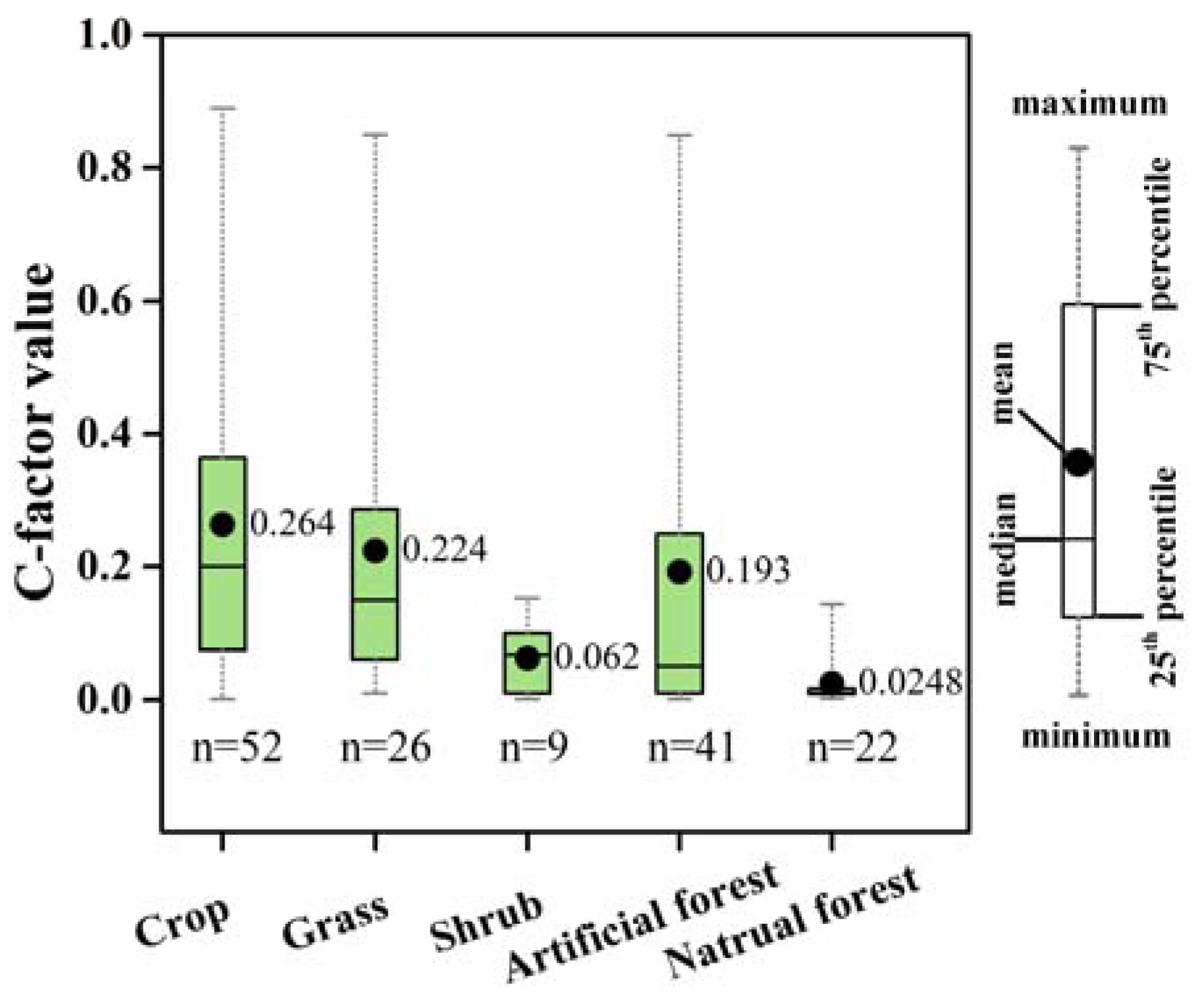
Here, we analyzed the C-factor values measured in field experiments. These field experiments were located in China, the USA, Japan, Portugal, Brazil, Belgium, Tanzania, Greece, and France. The majority of the plots in the field experiments followed the standard of USLE unit plots created by Wischmeier and Smith (1978) [10]. The C-factor values were estimated according to Equation (1). Figure 2 shows the C values derived from existing datasets for crops, grass, shrubs, and forests.
Figure 2 shows that there was a high degree of variability in the measured C-factor values. Specifically, the C-factor values of crops had the widest range, compared to other land-use types. The smallest C-factor value was observed for natural forest (0.0248 ± 0.0367), followed by shrubs (0.0622 ± 0.0525), artificial forest (0.193 ± 0.263), grass (0.224 ± 0.223), and crops (0.264 ± 0.228). The results indicate that natural vegetation was most effective in controlling soil erosion. The C-factor values based on field experiments can provide a valuable reference and benchmarking dataset for C.

4. Quantification of C-Factor for USLE-Type Modeling

4.1. Methods for Quantifying the C-Factor Values

Normally, the C-factor is estimated from long-term field experiments. However, because of the absence of experiments, various methods have been developed to quantify the C-factor for USLE-type modeling in the literature. A simple and widely used method is referencing studies that have reported C-factor values for similar land cover. In addition, many studies have reported various formulas for deriving C-factor values [6,16,19,21,22,23]. In general, the methods for calculating C-factor values can be classified into six categories: (1) C-factor estimated based on subfactors (M1); (2) C-factor estimated according to land cover classifications (M2); (3) C-factor estimated by vegetation indices (VIs) (M3); (4) C-factor estimated by vegetation coverage (VC) (M4); (5) C-factor estimated by spectral mixture analysis (SMA) (M5); and (6) C-factor estimated based on other methods (M6). The six types of methods are described and discussed in detail below.

4.1.1. C-Factor Estimation Based on Subfactors (M1)

Following the RUSLE handbook, the C-factor is computed of five subfactors [9] as following Equation (2):
C = PLU × CC × SC × SR × SM
where PLU is the land-use subfactor, CC is the canopy cover subfactor, SC is the surface cover subfactor, SR is the surface roughness subfactor, and SM is the soil moisture subfactor [9]. Individual subfactors are expressed as functions of more variables, so this method requires details of the cover characteristics including canopy cover, canopy height, and prior cropping [7], which are mainly used in field level investigations [24,25,26]. It is evident that Equation (2) is not feasible for large-scale investigations, because of the data availability [6]. Hence, the C-factor value has been calculated from VC through the CC subfactor for large-scale soil erosion modeling in some studies [27,28,29] as Equation (3):
C = CC = 1 f c × exp 0.0305 × H
where fc is the fraction of the land surface covered by canopy, and H (m) is the distance that raindrops fall after striking the canopy [9].

4.1.2. C-Factor Estimated According to Land Cover Classification (M2)

In most of the previous studies, the C-factor values were determined for each corresponding type of land use, and the values were obtained from available experimental data as tabulated in previous research works [30,31,32,33]. This simplified method assumes that the same land covers have the same values [7], and has been widely applied for large-scale soil erosion modeling, including the country-scale soil erosion assessment in Australia [34,35], South Korea [36], North Korea [37], Hungary [38,39] and even for global-scale modeling [40,41]. In addition, the C-factor values were also assigned to corresponding crop types in certain cases [30,42,43]. For example, Borrelli et al. (2017) determined C-factor values for fourteen crop groups (including 170 crops) according to the literature thresholds [17].
Here, we found 479 out of 946 studies had adopted empirical C-factor values for different land-use types according to previous research works (M2 method). There was a high degree of variability in the reported C-factor values among each type of land use (Figure 3). Specifically, the C-factor values for bare land and urban/village had the widest range (0–1), compared to other land-use types. The smallest C-factor value was observed for natural forest (0.013 ± 0.013), followed by wetlands (0.059 ± 0.105), shrub (0.092 ± 0.140), grass (0.105 ± 0.112), artificial forest (0.113 ± 0.142), sparse vegetation (0.207 ± 0.167), urban or village (0.22 ± 0.335), and crop (0.301 ± 0.114). The mean value reported for bare land was 0.58 (SD = 0.389). The C-factor values generally agree with those from field experiments (Figure 3). The observed smallest and largest C-factor values were associated with different land use types. The smallest C-factor value was found for natural forest. This can be attributed to the dense vegetation cover and complex root systems present in natural forests, which effectively reduce soil erosion. On the other hand, the largest C-factor values were observed for bare land and urban/village. These land use types often have minimal or no vegetation cover, resulting in high vulnerability to erosion processes. Factors such as land management, topography, climate, and conservation measures influence C-factor variations [7]. Moreover, the reported values represent the observed range and may differ based on geography and research methods. Further investigation is needed to understand the specific reasons for C-factor variations within each land use type and their impact on soil erosion processes.
The results indicate that the reported C-factor values generally align with those obtained from field experiments, as depicted in Figure 3. Furthermore, these results highlight the considerable variability in C-factor values across different land-use types and emphasize the need for accurate and context-specific estimations. The agreement between the reported C-factor values and those from field experiments strengthens the reliability of the empirical values used in our study.

4.1.3. C-Factor Estimated by Vegetation Indices (M3)

Previous studies have proposed several empirical equations that relate VIs to C-factor values. The most commonly used VIs was the Normalized Difference Vegetation Index (NDVI) [21,44,45], and linear relations between C-factor value and NDVI were fitted, which had been used in different regions as following equations [46,47,48,49,50,51,52,53]:
C = 0.431 0.805 × N D V I
C = 1.02 1.21 N D V I
C = 1.2079 4.6133 N D V I
C = 0.9167 1.1667 N D V I
C = 1 N D V I / 2
C = 0.407 0.5953 N D V I
C = 1.056 1.612 N D V I
C = 0.1 × 1 N D V I / 2
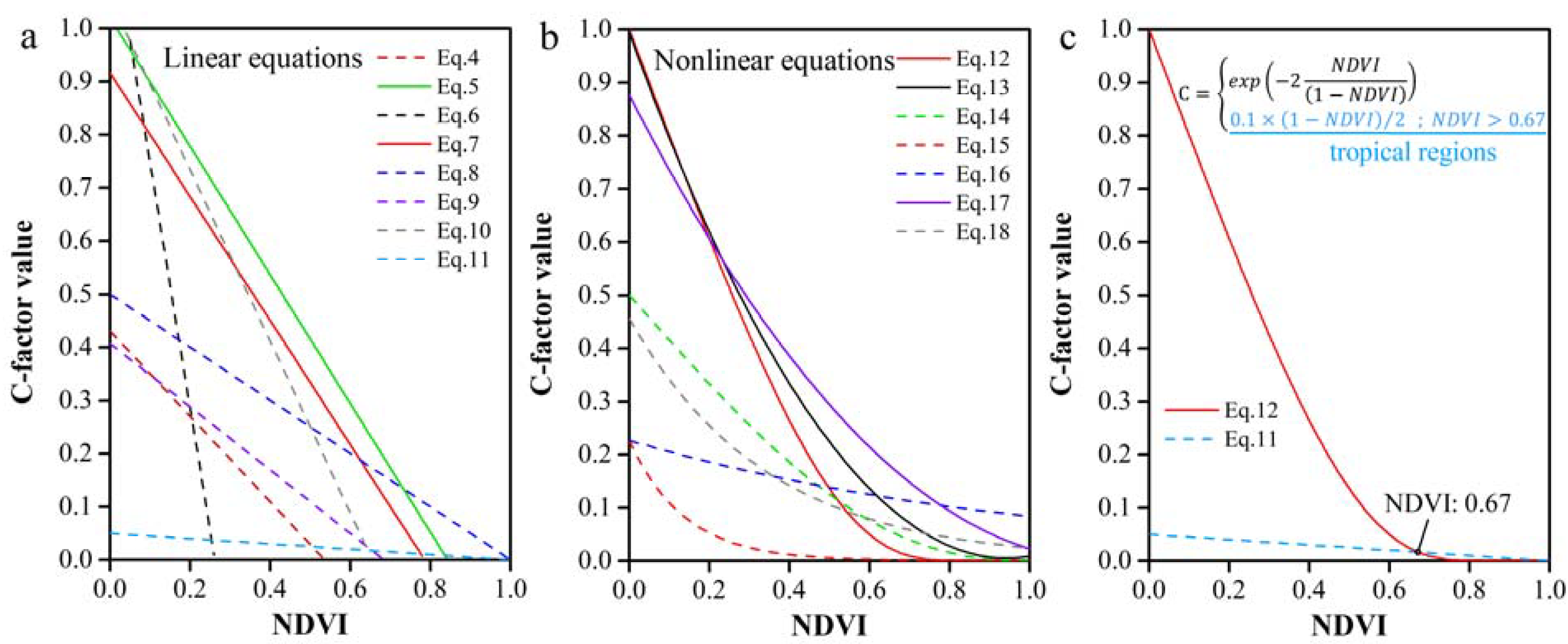
The Equations (4), (8) and (9) only hold valid for photosynthetic and not senescent vegetations [46] and are unable to predict C-factor values over 0.5 (Figure 4a), while Equations (6) and (10) are unable to predict the differences of C-factor values when the NDVI is over 0.26 and 0.68, respectively. The C-factor values calculated by Equations (5) and (7) tend to be larger under natural vegetation conditions with a high NDVI. In 2018,Colman performed a comparison between the C-factor values estimated by NDVI and those computed with experimental plots in Brazil [53,54], and found a 10-fold systematic bias from Equation (8) [50]. Hence, Colman recommended that Equation (11) was suitable in tropical regions [55]. Due to these limitations, the linear equations were used in very limited studies [56,57,58].
There are various nonlinear relationships between the NDVI and the C-factor value have been proposed as following (Figure 4b) [59,60,61,62,63,64,65]:
C = e x p 2 N D V I 1 N D V I
C = 1.1119 N D V I 2 2.0976 N D V I + 0.9944
C = 1 N D V I / 2 1 + N D V I
C = 0.227 e x p 7.337 N D V I
C = 0.227 e x p 0.997 N D V I
C = 0.625 N D V I 2 1.4793 N D V I + 0.8771
C = e x p 2.9298 N D V I 0.7842
Van der Knijff et al. developed Equation (12), which has been widely used to compute C-factor values [59,66,67,68,69,70]. However, the C-factor values calculated by Equation (12) tend to be smaller in tropical climate zones with more intense rainfall [50]. Almagro et al. compared Equations (11) and (12), and found that Equation (12) was not suitable to estimate the C-factor for most land uses, presenting larger values than those from experiments [55]. The C-factor values of polynomial equations (Equations (13) and (17)) indicate an overestimation related to land uses with a relatively high NDVI (Figure 4b). The power equation (Equation (14)) and exponential equations (Equations (15), (16) and (18)) are unable to predict C-factor values over 0.5 (Figure 4b), which means that these equations are limited in land uses with relatively high C-factor values, such as croplands.
The NDVI has a high correlation with the Leaf Area Index (LAI) [71], making it possible to estimate C-factor values through LAI as the flowing equation [72]:
C = 1.005 × e x p 0.426 P V I + 0.012
However, there are some issues associated with the NDVI and the LAI, due to the effects of soil reflectance, the sensitivity to vegetation conditions, etc. [21]. Hence, several alternative VIs have been used to quantify the C-factor [72,73]. For example, Yoshino and Ishioka developed a regression model to estimate C-factor values using the perpendicular vegetation index (PVI) [71]:
C = e x p 7.291 E V I
The enhanced vegetation index (EVI) was also employed to estimate the C-factor value [73], while the transformed soil adjusted vegetation index (TSAVI) has been recommended for use in arid and semi-arid areas [74,75].
C = 0.177 × ln L A I + 0.184
Feng et al. found that the C-factor is sensitive to yellow VIs, such as the normalized difference tillage index (NDTI) and the normalized difference senescent vegetation index (NDSVI) [21]. The normalized bare soil index (NBIL) and the modified soil-adjusted vegetation index (MSAVI) have also been used to calculate the C-factor [76,77].

4.1.4. C-Factor Estimated by Vegetation Coverage (M4)

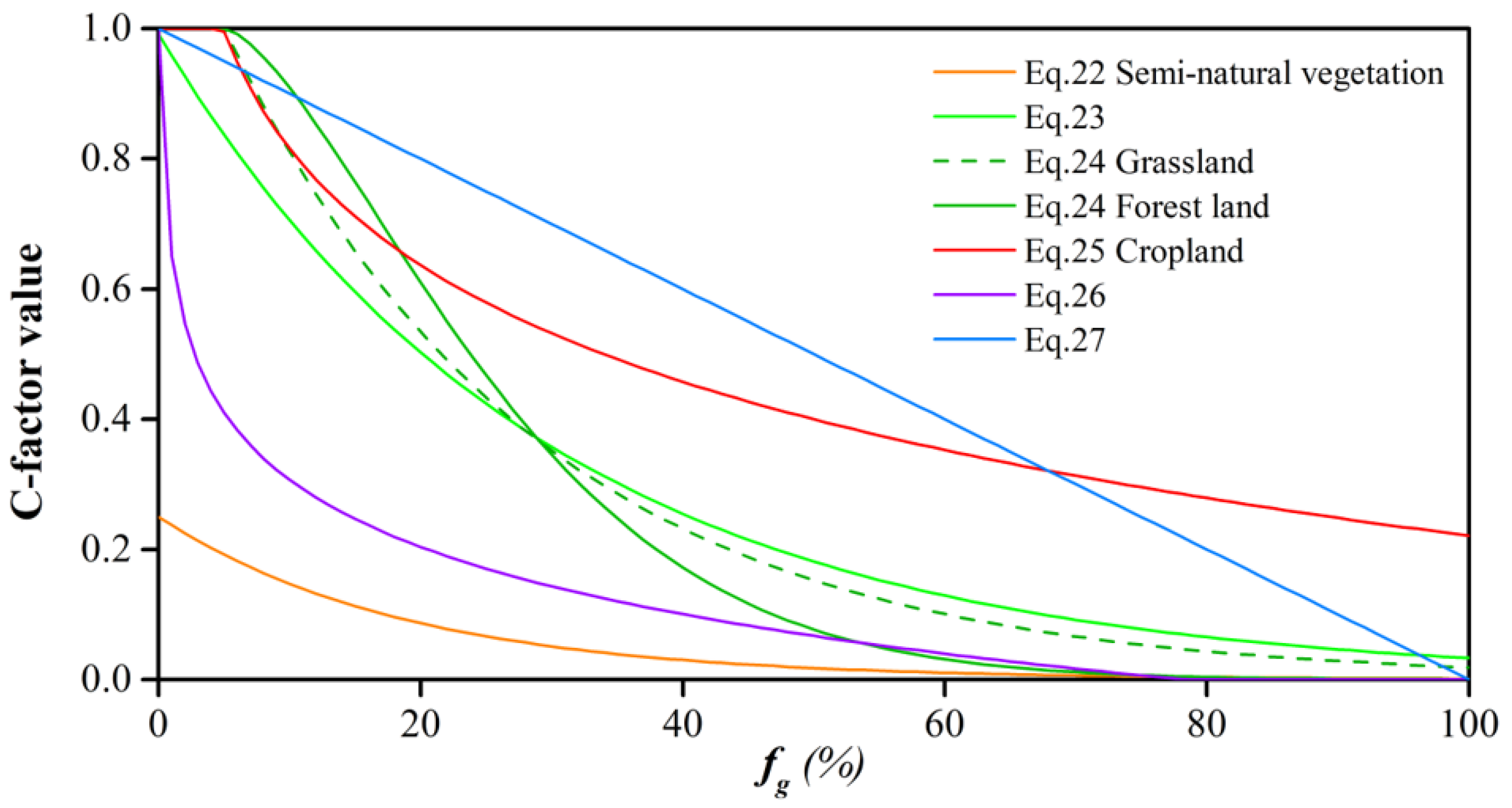
Vegetation coverage (VC) is also a dependable index for estimating the C-factor [78]. Thus, several alternative approaches based on VC have been established to quantify the C-factor as the following equations (Figure 5) [79,80,81,82,83,84]:
C = 0.25 × e x p 0.0529 f g
C = 0.992 × e x p 0.034 f g
C =   e x p 0.0418 f g 5 f g > 5 , Grassland e x p 0.0085 f g 5 1.5 f g > 5 , Forest land 1 f g 5
C = 0.221 0.595 log ( f g / 100 )
C = 1 f g = 0 0.6508 0.3436 lg f g 0 < f g 78.3 0 f g > 78.3
C = 1 0.01 f g
where fg is the VC (%). Among these, Equation (26) developed by Cai et al. has been used to estimate the C-factor values for all land-use types in many studies in China [79,85,86,87,88,89,90]. However, Equation (26) was developed based on runoff plots of croplands and orchards [79], the Equation (22) was developed based on semi natural vegetation [80], the Equation (24) was developed based on grassland and forest land [82], which means the accuracy of the estimated C-factor values for other land-use types cannot be ensured. For large-scale studies, the VC was often calculated using the NDVI derived from the MODIS images:
f g = 100 × N D V I N D V I m i n N D V I m a x N D V I m i n
where fg is the VC (%), NDVImax refers to the regional maximum NDVI, NDVImin is the NDVI of bare soil [91]. In some cases, the cumulative percentages of 5% and 95% were used to determine the corresponding values of NDVImin and NDVImax [21]. In addition, a linear relationship exists between fg and NDVI (Equation (29)) [92], which has also been used for C-factor estimation [88].
f g = 108.49 × NDVI + 0.717

4.1.5. C-Factor Estimated by Spectral Mixture Analysis (M5)

As an alternative to NDVI-based approaches, spectral mixture analysis (SMA) of Landsat ETM data can estimate the fractional abundance of vegetation, and have been used to quantify the C-factor [93,94,95]. Lu et al. developed Equation (30) to estimate the C-factor [96].
C = f s o i l 1 + f g v + f s h a d e + f g v × f s h a d e
where fsoil is the fraction of soil, fgv is the fraction of green vegetation, and fshade is the fraction of shade.
De Asis and Omasa presented a linear SMA (LSMA) to map the C-factor, which used the fractional abundance of bare soil and ground cover to estimate the C-factor on a pixel-by-pixel basis [8]:
C = f s o i l 1 + f g v + f N P M
where fNPM is the fraction of non-photosynthetic materials. De Asis and Omasa compared the C-factor among the LSMA-derived method (Equation (31)), the NDVI-derived method (Equation (4)), and field experiments in the Philippines [8]. The results showed that the LSMA-derived values correlated more strongly with the field-measured values, and the LSMA-derived C-factor showed a more detailed spatial variability, which indicated that this method can generate a more reliable estimate of soil erosion. However, there are some limitations of the SMA-derived C-factor; for example, this method assumes that its value is 0 under densely vegetated areas, which could lead to underestimated soil erosion in those areas [8].

4.1.6. C-Factor Estimation Based on other Methods (M6)

Traditionally, C-factor values are simply determined based on the literature or field data. Such methods assume that the same land-cover class has the same C-factor value [7,96]. However, the C-factor is largely related to vegetation conditions. Panagos et al. proposed a method for C-factor estimation (Equations (32) and (33)), which considers the combined effects of land-use type and VC [7].
C = M i n C l a n d u s e + M a x C l a n d u s e M i n C l a n d u s e × 1 F c o v e r
where Fcover is the percentage of land covered by vegetation; Clanduse is the value of each land-use type according to the literature data. The C-factor reaches its maximum value with Fcover = 0 (i.e., no vegetation), while it reaches its minimum with Fcover = 1 (i.e., land is fully covered by vegetation). However, the Fcover is not appropriate for croplands, as the VC changes during the year. Hence, this method has been used to estimate the C-factor for non-arable lands [7,17,97].
For arable lands, the C values of cropland in each country were calculated using following formula:
C crop = n = 1 14 C cropn ×   % Region Cropn
where Ccropn represents the C-factor of the n-crop and %RegionCropn represents the share of this crop in the agricultural land of the given region [7].
In some cases, the C-factor and P-factor (support practice factor) have been treated together as the CP factor [4,98,99,100,101,102,103,104,105,106,107]. For a managed artificial forest, the C-factor is closely related to the forest’s age [108].

4.2. Application of the Methods for C-Factor Quantification

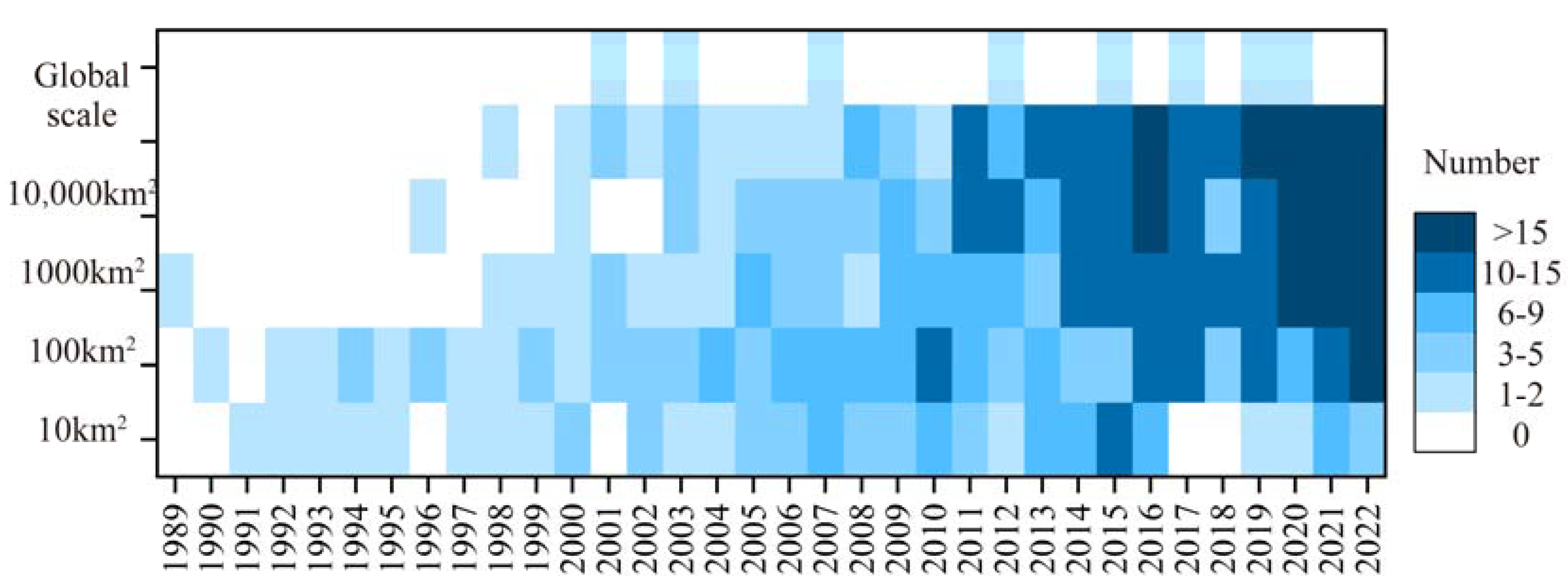
Figure 6 shows the size of the study area and the publication year of the 946 studies. The study areas ranged from plot scale (1–100 m2) to global scale, and there was an increasing trend in the number of studies, with more studies focusing on large-scale assessments in recent years.
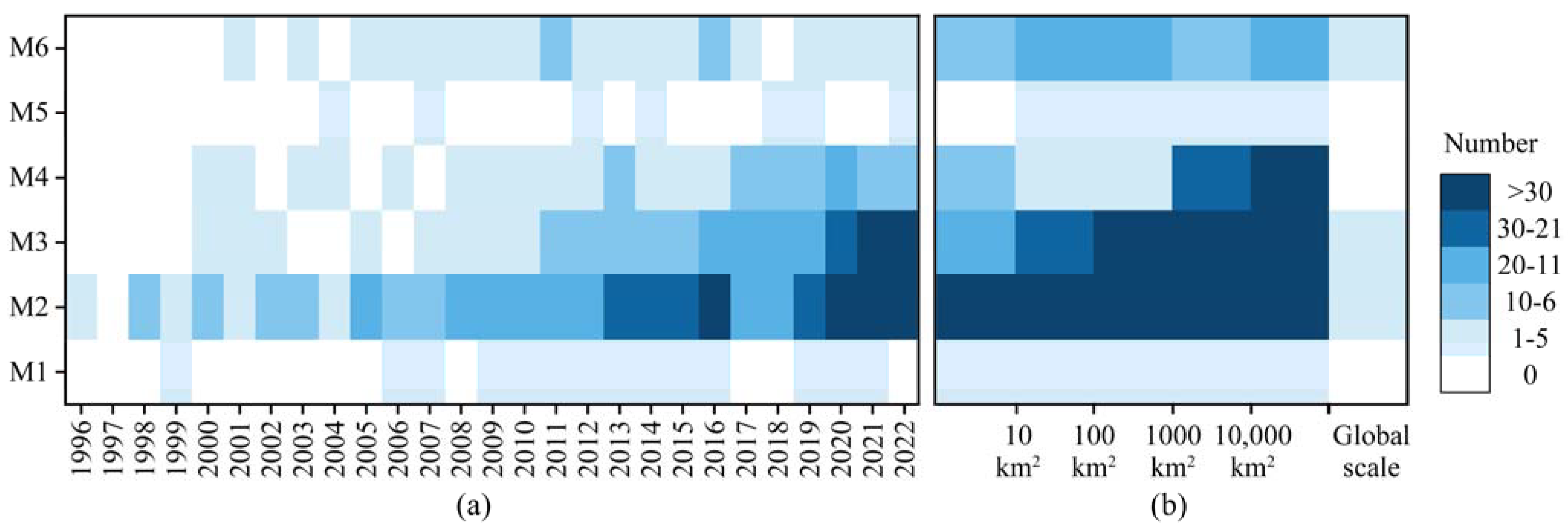
Figure 7a shows the number of studies using different methods for each year. Most studies adopted empirical uniform values for different land uses according to previous studies (M2 method, 478 studies) or calculated the C-factor based on the VIs (M3 method, 254 studies) (Figure 7a). Most of the previous studies using the M2 and M3 methods were conducted in large study areas (>100 km2) (Figure 7b). The M2, M3, and M4 methods are often applied using remote sensing data, such that the seasonal cycle of the C-factor can be determined in large areas, which can help to identify the periods within the year with severe soil erosion (Ferreira and Panagopoulos 2014).

4.3. Comparison of the Methods of C-Factor for Large Study Areas

The M2 and M3 methods have been commonly used in large study areas (Figure 7b); we use the NDVI of the year 2015 from the Global Inventory Modeling and Mapping Studies (GIMMS) NDVI3g data to estimate the global C-factor values according to the equations (Equations (4)–(27)). The half-month NDVI was combined for yearly data (Supplementary Figure S1a) using the maximum value composite method. Additionally, the landcover of the year 2015 from ESA CCI-LC at a 300 m spatial resolution (Supplementary Figure S1b), and crop harvested area data of each country from the FAO database, were used to estimate the C-factor values according to the method of Panagos et al. [7].
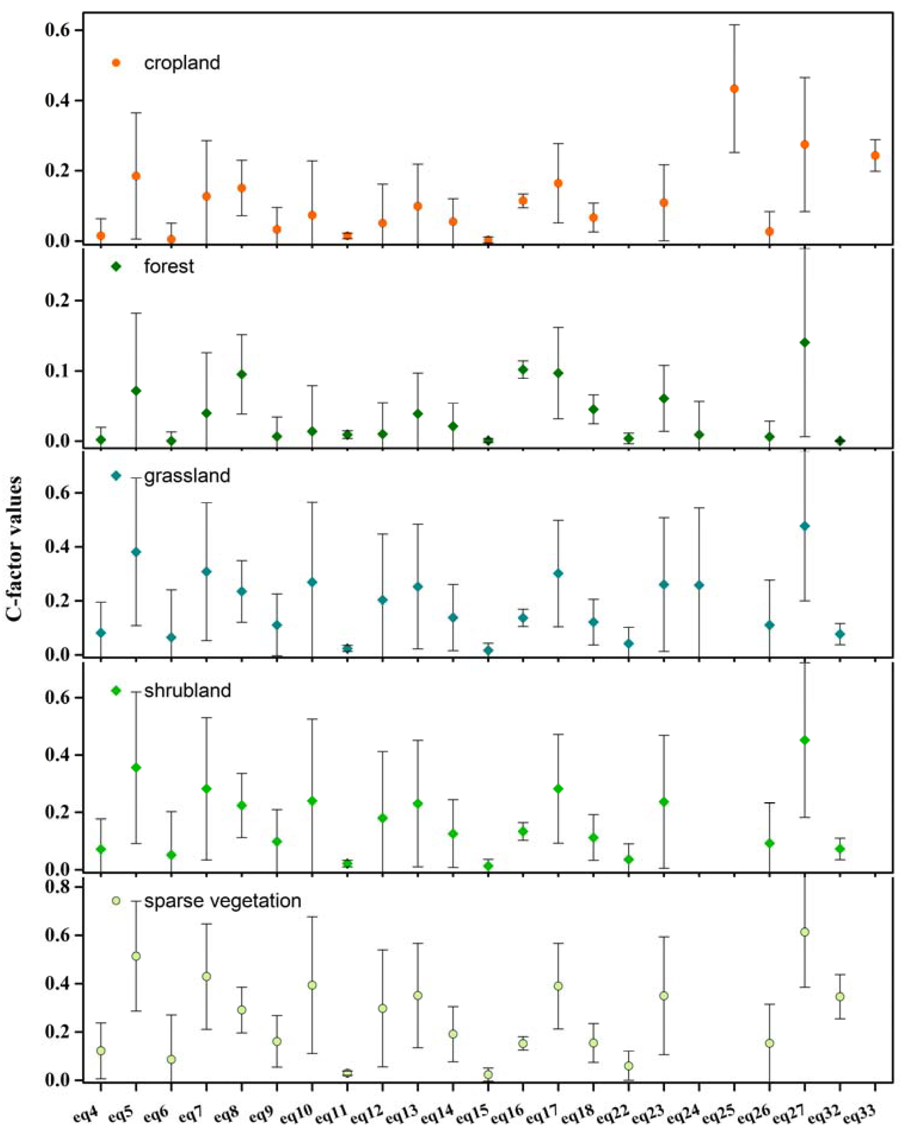
Figure 8 shows the mean and standard deviation for C-factor values of cropland, forest, grassland, shrubland, and sparse vegetation for the year 2015. The data demonstrate a high degree of variation in C-factor values among different land uses (Figure 8 and Figure S2 and Table S1). The mean C-factor value for cropland based on field experiments was found to be 0.264 (SD = 0.228) (Figure 3), which was greater than those obtained from theoretical equations, including Equations (4)–(18), (23), and (26). Additionally, the mean C-factor value for cropland, as estimated by Equation (25), was 0.434 (Figure 8 and Supplementary Table S1), indicating that the aforementioned equations were not effective for estimating the C-factor values of croplands on a large scale. The results of the study indicate that Equations (33) and (27) are suitable for estimating the C-factor values of cropland, as the mean values obtained by these equations were 0.244 (SD = 0.045) and 0.275 (SD = 0.190), respectively, consistent with those derived from field experiments. However, when applied to natural vegetation (such as forest, grassland, and shrubland), the C-factor values calculated using Equation (27) were significantly higher than those reported in the historical literature. Therefore, Equation (27) is considered to be unsuitable for natural vegetation. The other equations employed in the study also exhibited limitations in accurately estimating C-factor values for all land uses. Specifically, the mean C-factor values for grass, shrub, and forest, calculated using Equations (8), (32), and (14), were 0.235 (SD = 0.115), 0.073 (SD = 0.037), and 0.0215 (SD = 0.032), respectively, and were consistent with the results obtained from field experiments. The results suggest that the combined use of Equations (33) or (27) for cropland, Equation (8) for grass, Equation (32) for shrub, and Equation (14) for forest can be applied at a global scale. These results provide valuable insights for researchers and practitioners seeking to estimate C-factor values for large-scale soil erosion assessments.

5. Discussions

Our systematic review summarizes the methods for calculating C-factor values adopted by 946 studies. The C-factor has experienced a process of simplification to assess the potential impact on soil erosion over larger areas [55]. The most widely used methods were the M2 (478 studies), M3 (254 studies), and M4 (101studies) methods.

5.1. Comparison of the Main Methods of C-Factor for USLE-Type Modeling

The M2 method assumes that the same types of land use have an equal C-factor value [7]. Due to its simplicity, it was the most widely used method, given the difficulties in collecting and processing all of the necessary parameters. However, the accuracy of the C-factor values estimated by the M2 method largely depend on the accuracy of land cover classification. In addition, the same type of land use would have different C-factor values, due to the spatial heterogeneity in vegetation density [6,19] or management practices [7] in large geographic areas.
The M3 method uses VIs to assess C-factor values. Despite the fact that this method is generally accepted and has been widely used, some studies found that there were low correlations between VIs and the C-factor [19]. For example, in the regions covered by non-photosynthetic vegetation (NPV), the correlations between VIs and the C-factor value are low [8,19], because dry and dead vegetation could still exert influences on the C-factor [109]. Yang et al. found that incorporating NPV information can significantly improve the accuracy of C-factor estimation for China’s Loess Plateau [110]. Moreover, C-factor estimation only through VIs tends to result in overestimation, because this method ignores the differences in types of land use with the same VIs [44]. Recently, combining different VIs has been proposed as an alternative strategy to address this issue [21,109]. For example, Puente et al. used thirty VIs to identify the reliable relation between VIs and measured C-factor values from long-term experiments in Mexico, and found that the correlation coefficients with conventional VIs (such as NDVI and EVI) were low in general, showing that current VIs could not provide all of the information of the vegetation required by erosion models [109]. Feng et al. compared the estimates of C-factor values based on various VIs in the Loess Plateau of China, and found that a combination of green VIs (NDVI, PVI, TSAVI, and EVI) and yellow VIs (NDTI and NDSVI) could greatly improve the accuracy of C-factor values than those based on a single VI [21].
The M4 method estimates C-factor values based on VC, and the equations have been mainly developed in China. Since the VC has often been represented by the NDVI, the M4 method shares similar weaknesses with the M3 method. Each equation of M3 and M4 (Equations (12)–(27)) may be suitable to estimate the C-factor for some land-use types, but not all land uses. The M5 method has shown promising application, due to its capability for detecting both the healthy (green) and non-photosynthetic (dry and dead) vegetation [111]. However, this method cannot be used in areas completely covered by vegetation [19,111]. Thus, the M5 method has only been adopted by a few studies (seven studies), and was further constrained by its complex calculation procedures [22].
Each method has its own strengths and weaknesses, and no single method can meet all of the requirements. The C-factor values measured on plots under natural rainfall conditions (Figure 2) showed that the same type of land use even with the same VIs or VC could lead to different C-factor values [7,112]. Hence, the use of the M3, M4, and M5 methods, without on-site knowledge, may produce uncertainties that can reduce the accuracy of soil erosion predictions and assessments. Overall, for small-scale studies, it is more feasible to quantify the C-factor through experiments, estimates based on subfactors (M1 method), or obtain values from the literature (M2 method). At large scales, the M3, M4, and M5 methods can contribute to identify the impacts of vegetation change on soil erosion potential, especially when considering sub-monthly, monthly, or yearly vegetation change [6]. Notably, the resolution of satellite images is a common issue that would impair the robustness of the three methods. For example, Meusburger et al. showed that the resolution of a satellite image could affect the derivation of VIs, with subsequent impacts on the estimation of C-factor values and soil erosion [113]. The choice of methods should depend on the scale of the area, the objective of the studies, and the availability of data. For a given large-scale region, it may be better to use different equations for various types of land use than use the same equation for all types.

5.2. C-Factor Estimation for USLE-Type Modeling at Large Scale

In previous studies, the C-factor has been mainly quantified using the M2 method at national or regional scales. However, these studies did not fully consider the C-factor for soil erosion assessment (Table 1), except for the study by Panagos et al. Specifically, Panagos et al. proposed a methodology for estimating the C-factor values using pan-European datasets, biophysical attributes, and census data for arable lands [7]. The C-factor value of arable lands was estimated using crop statistics (% of land per crop) and information on management practices such as conservation tillage and mulching. In non-arable lands, the C-factor was quantified by weighting the literature values according to the fraction of vegetation cover [7]. Borrelli et al. also used this method to calculate the C-factor values at the national scale (Table 1) [114].
In recent years, USLE-type models have been applied for soil erosion assessment on a global scale (Table 1). Pham et al. conducted the first study on global soil erosion estimates using the USLE model, in which uniform C-factor values were applied for different types of land use [40]; this method was also used in the studies by Yang et al. and Ito [41,133]. Scherer and Pfister and Doetterl et al. used a global crop-type abundance map to estimate C-factor values [138,139]. Recently, Naipal et al. calculated the C-factor according to Equation (4) [140], but produced a positive bias in winter. Following previous pan-European studies [7], Borrelli et al. incorporated the types and spatial distribution of global croplands into a global USLE-type model [17,97]. Liu et al. quantified the C-factor according to Equation (12) [141].
Previous studies have shown that there are various crop management practices (CMPs, e.g., mulching, strip-cropping) on arable lands [142] and found that biological techniques can reduce the soil loss rate by around 88% based on a global analysis of runoff plots. Prosdocimi et al. reported the beneficial effects of mulching in reducing soil erosion by up to 90% [143]. Conservation agriculture occupies approximately 15% of global cropland [17], with CMPs widely applied in erosion-sensitive regions. However, the effects of CMPs on soil erosion were not fully considered in existing C-factor estimation methods.

5.3. Limitations and Future Improvements

Determination of the C-factor value is difficult, due to its dependence on many parameters such as the land cover, vegetative canopy cover, soil biomass, and surface roughness [16,19,128]. Our systematic literature review and analysis revealed several limitations in current estimations of C-factor values.
First, no single method is applicable in all regions and meets all of the requirements, especially for global-scale investigations. Second, the effects of CMPs have not been fully considered for croplands in existing C-factor estimation methods. Third, the estimated C-factor values based on VIs (Equations (12)–(21)) and VC (Equations (22)–(27)) were not well validated in field experiments, and each equation based on VIs and VC may be suitable to estimate the C-factor for some land-use types, but not all land uses. Indeed, different types of land use with even the same VIs or VC could have different C-factor values. Fourth, the accuracy of the C-factor value largely depends on the quality of the satellite images, as the land cover classification and VIs were directly derived from satellite images. High-resolution images can offer the advantage of capturing fine-scale details and accurately differentiating between various land cover types and vegetation densities. This allows for a more precise estimation of the C-factor by taking into account variations in vegetation cover. However, coarse spatial resolution satellite images, such as Landsat, are commonly used, as fine-resolution satellite images that can detect conservation practices are not freely available.
Here, we identify four key areas that require further efforts for improving the estimation of C-factor values: (1) Building regional and global scale C-factor databases through the collection and integration of field experiment data; (2) leveraging high-resolution satellite imagery and advanced image processing techniques for C-factor quantification; (3) combining multiple methods to enhance the robustness of soil erosion assessment; (4) strengthening the quantification of the uncertainty of C-factor values.

6. Conclusions

This study contributes a comprehensive database encompassing C-factor values, quantification methods, and study sites derived from an extensive analysis of 946 published articles. The increasing trend in studies focused on soil erosion assessment in recent years and the development of numerous methods to determine C-factor values indicate the importance of this research area. Our findings demonstrate that LUMPs play a significant role in mitigating soil erosion, with natural vegetation emerging as the most effective land use type. Through meticulous examination, we identified six prominent approaches for quantifying C-factor values, each carrying distinct advantages and limitations, indicating that a combination of methods is required for the robust estimation of C-factor values for different land-use types. We recommend the combined use of specific equations for cropland, grass, shrub, and forest to estimate C-factor values at the global scale. Further efforts are necessary to develop C-factor datasets at large scales by synthesizing field-level experiment data and combining high-resolution satellite imagery. The results of this study provide useful implications for C-factor quantification at various spatial scales and significantly improve our understanding of the uncertainties involved in soil erosion assessment using USLE-type models. These findings can inform decision-making processes and provide valuable guidance for soil conservation strategies, contributing to sustainable land use and environmental protection.

Supplementary Materials

The following supporting information can be downloaded at: https://www.mdpi.com/article/10.3390/rs15112868/s1, Figure S1: Spatial distribution of landcover and NDVI of the year 2015; Figure S2: Spatial distribution of C-factor values according to equations; Table S1: Mean and standard deviation (SD) for C-factor value per land use type.

Author Contributions

Conceptualization, M.X.; methodology, M.X.; writing—original draft preparation, M.X.; writing—review and editing, G.L. and Q.T. All authors have read and agreed to the published version of the manuscript.

Funding

This study is supported by the National Natural Science Foundation of China (42201116) and the Third Xinjiang Scientific Expedition and Research (2021xjkk0805).

Institutional Review Board Statement

Not applicable.

Informed Consent Statement

Not applicable.

Data Availability Statement

The data that support the findings of this study are available from the corresponding author upon reasonable request.

Conflicts of Interest

The authors declare no conflict of interest.

References

  1. Borrelli, P.; Panagos, P.; Langhammer, J.; Apostol, B.; Schütt, B. Assessment of the cover changes and the soil loss potential in European forestland: First approach to derive indicators to capture the ecological impacts on soil-related forest ecosystems. Ecol. Indic. 2016, 60, 1208–1220. [Google Scholar] [CrossRef]
  2. García-Ruiz, J.M.; Beguería, S.; Lanarenault, N.; Nadal-Romero, E.; Cerdà, A. Ongoing and Emerging Questions in Water Erosion Studies. Land Degrad. Dev. 2017, 28, 5–21. [Google Scholar] [CrossRef]
  3. Zhang, K.; Yu, Y.; Dong, J.; Yang, Q.; Xu, X. Adapting & testing use of USLE K factor for agricultural soils in China. Agric. Ecosyst. Environ. 2018, 269, 148–155. [Google Scholar] [CrossRef]
  4. Xiong, M.; Sun, R.; Chen, L. Global analysis of support practices in USLE-based soil erosion modeling. Prog. Phys. Geogr. Earth Environ. 2019, 43, 391–409. [Google Scholar] [CrossRef]
  5. Karydas, C.G.; Panagos, P.; Gitas, I.Z. A classification of water erosion models according to their geospatial char-acteristics. Int. J. Digit. Earth 2014, 7, 229–250. [Google Scholar] [CrossRef]
  6. Benavidez, R.; Jackson, B.; Maxwell, D.; Norton, K. A review of the (Revised) Universal Soil Loss Equation ((R)USLE): With a view to increasing its global applicability and improving soil loss estimates. Hydrol. Earth Syst. Sci. 2018, 22, 6059–6086. [Google Scholar] [CrossRef]
  7. Panagos, P.; Borrelli, P.; Meusburger, K.; Alewell, C.; Lugato, E.; Montanarella, L. Estimating the soil erosion cover-management factor at the European scale. Land Use Policy 2015, 48, 38–50. [Google Scholar] [CrossRef]
  8. de Asis, A.M.; Omasa, K. Estimation of vegetation parameter for modeling soil erosion using linear Spectral Mixture Analysis of Landsat ETM data. ISPRS J. Photogramm. Remote Sens. 2007, 62, 309–324. [Google Scholar] [CrossRef]
  9. Renard, K.G.; Foster, G.R.; McCool, W.D.K.; Yoder, D.C. Predicting Soil Erosion by Water: A Guide to Conservation Planning with the Revised Universal Soil Loss Equation; Agricultural Handbook 703; United States Departmetn of Agriculture: Washington, DC, USA, 1997.
  10. Wischmeier, W.H.; Smith, D.D. Predicting Rainfall Erosion Losses: A Guide to Conservation Planning; Agricultural Handbook 537; Science and Education Administration, U.S. Dept. of Agriculture: Washington, DC, USA, 1978. [Google Scholar]
  11. de Jong, S.; Paracchini, M.; Bertolo, F.; Folving, S.; Megier, J.; de Roo, A. Regional assessment of soil erosion using the distributed model SEMMED and remotely sensed data. Catena 1999, 37, 291–308. [Google Scholar] [CrossRef]
  12. NSERL. WEPP User Summary; National Soil Erosion Research Laboratory, US Department of Agriculture: West Lafayette, IN, USA, 1995. [Google Scholar]
  13. Arnold, J.G.; Moriasi, D.N.; Gassman, P.W.; Abbaspour, K.C.; White, M.J. SWAT: Model use, calibration, and vali-dation. Am. Soc. Agric. Biol. Eng. 2012, 55, 1491–1508. [Google Scholar]
  14. Bangash, R.F.; Passuello, A.; Sanchez-Canales, M.; Terrado, M.; López, A.; Elorza, F.J.; Ziv, G.; Acuña, V.; Schuhmacher, M. Ecosystem services in Mediterranean river basin: Climate change impact on water provisioning and erosion control. Sci. Total Environ. 2013, 458–460, 246–255. [Google Scholar] [CrossRef] [PubMed]
  15. Cilek, A.; Berberoglu, S.; Kirkby, M.; Irvine, B.; Donmez, C.; Erdogan, M. Erosion Modelling In A Mediterranean Subcatchment Under Climate Change Scenarios Using Pan-European Soil Erosion Risk Assessment (PESERA). ISPRS Int. Arch. Photogramm. Remote Sens. Spat. Inf. Sci. 2015, XL-7/W3, 359–365. [Google Scholar] [CrossRef]
  16. Alewell, C.; Borrelli, P.; Meusburger, K.; Panagos, P. Using the USLE: Chances, challenges and limitations of soil erosion modelling. Int. Soil Water Conserv. Res. 2019, 7, 203–225. [Google Scholar] [CrossRef]
  17. Borrelli, P.; Robinson, D.A.; Fleischer, L.R.; Lugato, E.; Ballabio, C.; Alewell, C.; Meusburger, K.; Modugno, S.; Schütt, B.; Ferro, V.; et al. An assessment of the global impact of 21st century land use change on soil erosion. Nat. Commun. 2017, 8, 2013. [Google Scholar] [CrossRef]
  18. Panagos, P.; Borrelli, P.; Poesen, J.; Ballabio, C.; Lugato, E.; Meusburger, K.; Montanarella, L.; Alewell, C. The new assessment of soil loss by water erosion in Europe. Environ. Sci. Policy 2015, 54, 438–447. [Google Scholar] [CrossRef]
  19. Phinzi, K.; Ngetar, N.S. The assessment of water-borne erosion at catchment level using GIS-based RUSLE and remote sensing: A review. Int. Soil Water Conserv. Res. 2019, 7, 27–46. [Google Scholar] [CrossRef]
  20. Kinnell, P. Event soil loss, runoff and the Universal Soil Loss Equation family of models: A review. J. Hydrol. 2010, 385, 384–397. [Google Scholar] [CrossRef]
  21. Feng, Q.; Zhao, W.; Ding, J.; Fang, X.; Zhang, X. Estimation of the cover and management factor based on stratified coverage and remote sensing indices: A case study in the Loess Plateau of China. J. Soils Sediments 2018, 18, 775–790. [Google Scholar] [CrossRef]
  22. Feng, Q.; Zhao, W.W. The study on cover-management factor in USLE and RUSLE: A review. Acta Ecol. Sin. 2014, 34, 4461–4472. [Google Scholar]
  23. Vatandaslar, C.; Yavuz, M. Modeling cover management factor of RUSLE using very high-resolution satellite im-agery in a semiarid watershed. Environ. Earth Sci. 2017, 76, 65. [Google Scholar] [CrossRef]
  24. Arnhold, S.; Lindner, S.; Lee, B.; Martin, E.; Kettering, J.; Trung Thanh, N.; Koellner, T.; Ok, Y.S.; Huwe, B. Conven-tional and organic farming: Soil erosion and conservation potential for row crop cultivation. Geoderma 2014, 219, 89–105. [Google Scholar] [CrossRef]
  25. Fernández, C.; Vega, J.A.; Vieira, D. Assessing soil erosion after fire and rehabilitation treatments in NW Spain: Performance of rusle and revised Morgan-Morgan-Finney models. Land Degrad. Dev. 2010, 21, 58–67. [Google Scholar] [CrossRef]
  26. Zhang, H.; Wang, Q.; Dai, L.; Shao, G.; Tang, L.; Wang, S.; Gu, H. Quantifying soil erosion with GIS-based RUSLE under different forest management options in Jianchang Forest Farm. Sci. China Technol. Sci. 2006, 49, 160–166. [Google Scholar] [CrossRef]
  27. Mallick, J.; Alashker, Y.; Mohammad, S.A.-D.; Ahmed, M.; Hasan, M.A. Risk assessment of soil erosion in semi-arid mountainous watershed in Saudi Arabia by RUSLE model coupled with remote sensing and GIS. Geocarto Int. 2014, 29, 915–940. [Google Scholar] [CrossRef]
  28. Naqvi, H.R.; Mallick, J.; Devi, L.M.; Siddiqui, M.A. Multi-temporal annual soil loss risk mapping employing Revised Universal Soil Loss Equation (RUSLE) model in Nun Nadi Watershed, Uttrakhand (India). Arab. J. Geosci. 2012, 6, 4045–4056. [Google Scholar] [CrossRef]
  29. Zhou, P.; Nieminen, J.; Tokola, T.; Luukkanen, O.; Oliver, T. Large scale soil erosion modeling for a mountainous watershed. In Geo-Environment and Landscape Evolution II: Evolution, Monitoring, Simulation, Management and Remediation of the Geological Environment and Landscape; Wit Press: Billerica, MA, USA, 2006; pp. 55–66. [Google Scholar]
  30. Krasa, J.; Dostal, T.; Vrana, K.; Plocek, J. Predicting spatial patterns of sediment delivery and impacts of land-use scenarios on sediment transport in Czech catchments. Land Degrad. Dev. 2009, 21, 367–375. [Google Scholar] [CrossRef]
  31. Latocha, A.; Szymanowski, M.; Jeziorska, J.; Stec, M.; Roszczewska, M. Effects of land abandonment and climate change on soil erosion—An example from depopulated agricultural lands in the Sudetes Mts., SW Poland. Catena 2016, 145, 128–141. [Google Scholar] [CrossRef]
  32. Teng, H.; Liang, Z.; Chen, S.; Liu, Y.; Rossel, R.A.V.; Chappell, A.; Yu, W.; Shi, Z. Current and future assessments of soil erosion by water on the Tibetan Plateau based on RUSLE and CMIP5 climate models. Sci. Total Environ. 2018, 635, 673–686. [Google Scholar] [CrossRef]
  33. Villarreal, M.L.; Webb, R.H.; Norman, L.M.; Psillas, J.L.; Rosenberg, A.S.; Carmichael, S.; Petrakis, R.E.; Sparks, P.E. Modeling Landscape-scale Erosion Potential Related to Vehicle Disturbances Along the USA-Mexico Border. Land Degrad. Dev. 2014, 27, 1106–1121. [Google Scholar] [CrossRef]
  34. Lu, H.; Prosser, I.P.; Moran, C.J.; Gallant, J.C.; Priestley, G.; Stevenson, J.G. Predicting sheetwash and rill erosion over the Australian continent. Soil Res. 2003, 41, 1037–1062. [Google Scholar] [CrossRef]
  35. Teng, H.; Rossel, R.A.V.; Shi, Z.; Behrens, T.; Chappell, A.; Bui, E. Assimilating satellite imagery and visible–near infrared spectroscopy to model and map soil loss by water erosion in Australia. Environ. Model. Softw. 2015, 77, 156–167. [Google Scholar] [CrossRef]
  36. Park, S.; Oh, C.; Jeon, S.; Jung, H.; Choi, C. Soil erosion risk in Korean watersheds, assessed using the revised universal soil loss equation. J. Hydrol. 2011, 399, 263–273. [Google Scholar] [CrossRef]
  37. Lee, E.; Ahn, S.; Im, S. Estimation of soil erosion rate in the Democratic People’s Republic of Korea using the RUSLE model. For. Sci. Technol. 2017, 13, 100–108. [Google Scholar] [CrossRef]
  38. Pasztor, L.; Waltner, I.; Centeri, C.; Belenyesi, M.; Takacs, K. Soil erosion of Hungary assessed by spatially explicit modelling. J. Maps 2016, 12, 407–414. [Google Scholar] [CrossRef]
  39. Waltner, I.; Saeidi, S.; Grósz, J.; Centeri, C.; Laborczi, A.; Pásztor, L. Spatial Assessment of the Effects of Land Cover Change on Soil Erosion in Hungary from 1990 to 2018. ISPRS Int. J. Geo-Inf. 2020, 9, 667. [Google Scholar] [CrossRef]
  40. Pham, T.N.; Yang, D.; Kanae, S.; Oki, T.; Musiake, K. Application of RUSLE Model on Global Soil Erosion Estimate. Proc. Hydraul. Eng. 2001, 45, 811–816. [Google Scholar] [CrossRef]
  41. Yang, D.; Kanae, S.; Oki, T.; Koike, T.; Musiake, K. Global potential soil erosion with reference to land use and climate changes. Hydrol. Process. 2003, 17, 2913–2928. [Google Scholar] [CrossRef]
  42. SooHoo, W.M.; Wang, C.; Li, H. Geospatial assessment of bioenergy land use and its impacts on soil erosion in the U.S. Midwest. J. Environ. Manag. 2017, 190, 188–196. [Google Scholar] [CrossRef]
  43. Wijesundara, N.C.; Abeysingha, N.S.; Dissanayake, D.M.S.L.B. GIS-based soil loss estimation using RUSLE model: A case of Kirindi Oya river basin, Sri Lanka. Model. Earth Syst. Environ. 2018, 4, 251–262. [Google Scholar] [CrossRef]
  44. Yan, H.; Wang, L.; Wang, T.; Wang, Z.; Shi, Z. A synthesized approach for estimating the C-factor of RUSLE for a mixed-landscape watershed: A case study in the Gongshui watershed, southern China. Agric. Ecosyst. Environ. 2020, 301, 107009. [Google Scholar] [CrossRef]
  45. Liu, H.; Zhao, W.; Liu, Y. Assessment on the Soil Retention Service of Water Erosion in the Nile River Basin Considering Vegetation Factor Variance from 1982 to 2013. Water 2020, 12, 2018. [Google Scholar] [CrossRef]
  46. De Jong, S.M.; Brouwer, L.C.; Riezebos, H.T. Erosion Hazard Assessment in the Peyne Catchment, France; Utrecht University: Utrecht, The Netherlands, 1998. [Google Scholar]
  47. Demirci, A.; Karaburun, A. Estimation of soil erosion using RUSLE in a GIS framework: A case study in the Buyukcekmece Lake watershed, northwest Turkey. Environ. Earth Sci. 2011, 66, 903–913. [Google Scholar] [CrossRef]
  48. Jamshidi, R.; Dragovich, D.; Webb, A.A. Native forest C factor determination using satellite imagery in four sub-catchments. In Revisiting Experimental Catchment Studies in Forest Hydrology; IAHS Press: Wallingford, UK, 2012; pp. 64–73. [Google Scholar]
  49. Toumi, S.; Meddi, M.; Mahé, G.; Brou, Y.T. Remote sensing and GIS applied to the mapping of soil loss by erosion in the Wadi Mina catchment. Hydrol. Sci. J. 2013, 58, 1542–1558. [Google Scholar] [CrossRef]
  50. Durigon, V.L.; de Carvalho, D.F.; Antunes, M.A.H.; Oliveira, P.T.; Fernandes, M.M. NDVI time series for monitoring RUSLE cover management factor in a tropical watershed. Int. J. Remote Sens. 2014, 35, 441–453. [Google Scholar] [CrossRef]
  51. Fallah, M.; Kavian, A.; Omidvar, E. Watershed prioritization in order to implement soil and water conservation practices. Environ. Earth Sci. 2016, 75, 1248. [Google Scholar] [CrossRef]
  52. Joshi, V.U. Soil Loss Estimation based on RUSLE along the Central Hunter Valley Region, NSW, Australia. J. Geol. Soc. India 2018, 91, 554–562. [Google Scholar] [CrossRef]
  53. Colman, C.B. Impacts of Climate and Land Use Changes on Soil Erosion in the Upper Paraguay Basin; Federal University of Mato Grosso do Sul: Campo Grande, Brazil, 2018. [Google Scholar]
  54. Oliveira, P.T.S.; Nearing, M.A.; Wendland, E. Orders of magnitude increase in soil erosion associated with land use change from native to cultivated vegetation in a Brazilian savannah environment. Earth Surf. Process. Landforms 2015, 40, 1524–1532. [Google Scholar] [CrossRef]
  55. Almagro, A.; Thomé, T.C.; Colman, C.B.; Pereira, R.B.; Junior, J.M.; Rodrigues, D.B.B.; Oliveira, P.T.S. Improving cover and management factor (C-factor) estimation using remote sensing approaches for tropical regions. Int. Soil Water Conserv. Res. 2019, 7, 325–334. [Google Scholar] [CrossRef]
  56. Erencin, Z. C-Factor Mapping Using Remote Sensing and GIS: A Case Study of Lom Sak/Lom Kao, Thailand; Geographisches Institut der Justus-Liebig-Universität Giessen and Soil Science Division International Institute for Aerospace Survey and Earth Sciences: Enschede, The Netherlands, 2000. [Google Scholar]
  57. Gupita, D.D.; Murti, S.H.B.S. Soil erosion and its correlation with vegetation cover: An assesment using multispectral imagery and pixel-based geographic information system in Gesing Sub-Watershed, Central Java, Indonesia. In Proceedings of the 3rd International Symposium on LAPAN-IPB Satellite for Food Security and Environmental Monitoring 2016, Bogor, Indonesia, 25–26 October 2016; IOP Publishing Ltd.: Bristol, UK, 2017. [Google Scholar]
  58. Uddin, K.; Murthy, M.S.R.; Wahid, S.M.; Matin, M.A. Estimation of Soil Erosion Dynamics in the Koshi Basin Using GIS and Remote Sensing to Assess Priority Areas for Conservation. PLoS ONE 2016, 11, e0150494. [Google Scholar] [CrossRef]
  59. EUR 19022 EN; Soil Erosion Risk Assessment in Italy. European Soil Bureau: Ispra, Italy, 1999.
  60. Lin, C.-Y.; Lin, W.-T.; Chou, W.-C. Soil erosion prediction and sediment yield estimation: The Taiwan experience. Soil Tillage Res. 2002, 68, 143–152. [Google Scholar] [CrossRef]
  61. Mazour, M.; Roose, E. Influence de la couverture végétale sur le ruissellement et l’érosion des sols sur parcelles d’érosion dans des bassins versants du Nord-Ouest de l’Algérie. Bull. Réseau Eros. 2002, 21, 320–330. (In French) [Google Scholar]
  62. Suriyaprasita, M.; Shrestha, D.P. Deriving land use and canopy cover factor from remote sensing and field data in inaccessible mountainous terrain for use in soil erosion modeling. In International Archives of the Photogrammetry, Remote Sensing and Spatial Information Sciences; International Society for Photogrammetry and Remote Sensing: Beijing, China, 2008; pp. 1747–1750. [Google Scholar]
  63. Wickama, J.; Masselink, R.; Sterk, G. The effectiveness of soil conservation measures at a landscape scale in the West Usambara highlands, Tanzania. Geoderma 2015, 241–242, 168–179. [Google Scholar] [CrossRef]
  64. Bahrawi, J.A.; Elhag, M.; Aldhebiani, A.Y.; Galal, H.K.; Hegazy, A.K.; Alghailani, E. Soil Erosion Estimation Using Remote Sensing Techniques in Wadi Yalamlam Basin, Saudi Arabia. Adv. Mater. Sci. Eng. 2016, 2016, 9585962. [Google Scholar] [CrossRef]
  65. Kulikov, M.; Schickhoff, U.; Borchardt, P. Spatial and seasonal dynamics of soil loss ratio in mountain rangelands of south-western Kyrgyzstan. J. Mt. Sci. 2016, 13, 316–329. [Google Scholar] [CrossRef]
  66. Alexakis, D.D.; Hadjimitsis, D.G.; Agapiou, A. Integrated use of remote sensing, GIS and precipitation data for the assessment of soil erosion rate in the catchment area of “Yialias” in Cyprus. Atmos. Res. 2013, 131, 108–124. [Google Scholar] [CrossRef]
  67. Alexandridis, T.; Sotiropoulou, A.M.; Bilas, G.; Karapetsas, N.; Silleos, N.G. The effects of seasonality in estimating the C-factor of soil erosion studies. Land Degrad. Dev. 2015, 26, 596–603. [Google Scholar] [CrossRef]
  68. Guerra, C.A.; Maes, J.; Geijzendorffer, I.; Metzger, M.J. An assessment of soil erosion prevention by vegetation in Mediterranean Europe: Current trends of ecosystem service provision. Ecol. Indic. 2016, 60, 213–222. [Google Scholar] [CrossRef]
  69. Heung, B.; Bakker, L.; Schmidt, M.G.; Dragićević, S. Modelling the dynamics of soil redistribution induced by sheet erosion using the Universal Soil Loss Equation and cellular automata. Geoderma 2013, 202–203, 112–125. [Google Scholar] [CrossRef]
  70. Omuto, C.T.; Vargas, R.R. Combining pedometrics, remote sensing and field observations for assessing soil loss in challenging drylands: A case study of Northwestern Somalia. Land Degrad. Dev. 2008, 20, 101–115. [Google Scholar] [CrossRef]
  71. Yoshino, K.; Ishioka, Y. Guidelines for soil conservation towards integrated basin management for sustainable development: A new approach based on the assessment of soil loss risk using remote sensing and GIS. Paddy Water Environ. 2005, 3, 235–247. [Google Scholar] [CrossRef]
  72. Zhang, H.; Yu, D.; Dong, L.; Shi, X.; Warner, E.; Gu, Z.; Sun, J. Regional soil erosion assessment from remote sensing data in rehabilitated high density canopy forests of southern China. Catena 2014, 123, 106–112. [Google Scholar] [CrossRef]
  73. Kefi, M.; Yoshino, K.; Setiawan, Y. Assessment and mapping of soil erosion risk by water in Tunisia using time series MODIS data. Paddy Water Environ. 2011, 10, 59–73. [Google Scholar] [CrossRef]
  74. Hochschild, V.; Märker, M.; Rodolfi, G.; Staudenrausch, H. Delineation of erosion classes in semi-arid southern African grasslands using vegetation indices from optical remote sensing data. Hydrol. Process. 2003, 17, 917–928. [Google Scholar] [CrossRef]
  75. Kefi, M.; Yoshino, K.; Setiawan, Y.; Zayani, K.; Boufaroua, M. Assessment of the effects of vegetation on soil erosion risk by water: A case of study of the Batta watershed in Tunisia. Environ. Earth Sci. 2010, 64, 707–719. [Google Scholar] [CrossRef]
  76. Pinson, A.O.; AuBuchon, J.S. A new method for calculating C factor when projecting future soil loss using the Revised Universal soil loss equation (RUSLE) in semi-arid environments. Catena 2023, 226, 107067. [Google Scholar] [CrossRef]
  77. Roy, S.; Das, S.; Sengupta, S.; Mistry, S.; Chatterjee, J. Monitoring the temporal dimension of soil erosion in Mayurakshi Basin, India: A novel approach integrating RUSLE, Shannon’s entropy and landscape ecological metrics. J. Earth Syst. Sci. 2022, 131, 249. [Google Scholar] [CrossRef]
  78. Pal, S.C.; Chakrabortty, R. Simulating the impact of climate change on soil erosion in sub-tropical monsoon dom-inated watershed based on RUSLE, SCS runoff and MIROC5 climatic model. Adv. Space Res. 2019, 64, 352–377. [Google Scholar] [CrossRef]
  79. Cai, C.F.; Ding, S.W.; Shi, Z.H.; Huang, L.; Zhang, G.Y. Study of applying USLE and geographical information system IDRISI to predict soil erosion in small watershed. J. Soil Water Conserv. 2000, 14, 19–24. (In Chinese) [Google Scholar]
  80. Hurni, H. Erosion productivity conservation systems in Ethiopia. In Soil Conservation and Productivity, Proceedings of the 4th International Conference on Soil Conservation, Maracay, Venezuela, 3–9 November 1985; Sentis, I.P., Ed.; American Society of Agronomy, Inc.: Madison, WI, USA, 1985; pp. 654–674. [Google Scholar]
  81. Jin, Z.P.; Shi, P.J.; Hou, F.C. Soil Erosion System Model and Its Control Pattern in Huangfuchuan Valley of the Yellow River; The Ocean Press: Beijing, China, 1992. [Google Scholar]
  82. Jiang, Z.S.; Wang, Z.Q.; Liu, Z. Quantitative study on spatial variation of soil erosion in a small watershed in the Loess Hilly region. J. Soil Eros. Soil Conserv. 1996, 2, 2–9. (In Chinese) [Google Scholar]
  83. Liu, B.Z.; Liu, S.H.; Zheng, S.D. Soil conservation and coefficient of soil conservation of crops. Res. Soil Water Conserv. 1999, 6, 32–36. (In Chinese) [Google Scholar]
  84. Xu, L.; Xu, X.; Meng, X. Risk assessment of soil erosion in different rainfall scenarios by RUSLE model coupled with Information Diffusion Model: A case study of Bohai Rim, China. Catena 2013, 100, 74–82. [Google Scholar] [CrossRef]
  85. Shi, Z.H.; Cai, C.F.; Ding, S.W.; Wang, T.W.; Chow, T.L. Soil conservation planning at the small watershed level using RUSLE with GIS: A case study in the Three Gorge Area of China. Catena 2004, 55, 33–48. [Google Scholar] [CrossRef]
  86. Sun, W.; Shao, Q.; Liu, J.; Zhai, J. Assessing the effects of land use and topography on soil erosion on the Loess Plateau in China. Catena 2014, 121, 151–163. [Google Scholar] [CrossRef]
  87. Xiao, L.; Yang, X.; Chen, S.; Cai, H. An assessment of erosivity distribution and its influence on the effectiveness of land use conversion for reducing soil erosion in Jiangxi, China. Catena 2015, 125, 50–60. [Google Scholar] [CrossRef]
  88. Yang, M.; Li, X.; Hu, Y.; He, X. Assessing effects of landscape pattern on sediment yield using sediment delivery distributed model and a landscape indicator. Ecol. Indic. 2012, 22, 38–52. [Google Scholar] [CrossRef]
  89. Yao, H.; Shi, C.; Shao, W.; Bai, J.; Yang, H. Changes and influencing factors of the sediment load in the Xiliugou basin of the upper Yellow River, China. Catena 2016, 142, 1–10. [Google Scholar] [CrossRef]
  90. Zhou, P.; Luukkanen, O.; Tokola, T.; Nieminen, J. Effect of vegetation cover on soil erosion in a mountainous watershed. Catena 2008, 75, 319–325. [Google Scholar] [CrossRef]
  91. Fu, B.; Liu, Y.; Lü, Y.; He, C.; Zeng, Y.; Wu, B. Assessing the soil erosion control service of ecosystems change in the Loess Plateau of China. Ecol. Complex. 2011, 8, 284–293. [Google Scholar] [CrossRef]
  92. Ma, C.F.; Ma, J.W.; Aosaier, B. Quantitative assessment of vegetation coverage factor in USLE model using remote sensing data. Bull. Soil Water Conserv. 2001, 21, 6–9. (In Chinese) [Google Scholar]
  93. Huang, J.; Lu, D.; Li, J.; Wu, J.; Chen, S.; Zhao, W.; Ge, H.; Huang, X.; Yan, X. Integration of Remote Sensing and GIS for Evaluating Soil Erosion Risk in Northwestern Zhejiang, China. Photogramm. Eng. Remote Sens. 2012, 78, 935–946. [Google Scholar] [CrossRef]
  94. Jiang, Z.; Su, S.; Jing, C.; Lin, S.; Fei, X.; Wu, J. Spatiotemporal dynamics of soil erosion risk for Anji County, China. Stoch. Environ. Res. Risk Assess. 2012, 26, 751–763. [Google Scholar] [CrossRef]
  95. Pan, J.; Wen, Y. Estimation of soil erosion using RUSLE in Caijiamiao watershed, China. Nat. Hazards 2013, 71, 2187–2205. [Google Scholar] [CrossRef]
  96. Lu, D.; Li, G.; Valladares, G.S.; Batistella, M. Mapping soil erosion risk in Rondonia, Brazilian Amazonia: Using RULSE, remote sensing and GIS. Land Degrad. Dev. 2004, 15, 499–512. [Google Scholar] [CrossRef]
  97. Borrelli, P.; Robinson, D.A.; Panagos, P.; Lugato, E.; Yang, J.E.; Alewell, C.; Wuepper, D.; Montanarella, L.; Ballabio, C. Land use and climate change impacts on global soil erosion by water (2015–2070). Proc. Natl. Acad. Sci. USA 2020, 117, 21994–22001. [Google Scholar] [CrossRef]
  98. Andriyani, I.; Jourdain, D.; Lidon, B.; Soni, P.; Kartiwa, B. Upland farming system erosion yields and their constraints to change for sustainable agricultural conservation practices: A case study of land use and land cover (LULC) change in In-donesia. Land Degrad. Dev. 2017, 28, 421–430. [Google Scholar] [CrossRef]
  99. Bhandari, K.P.; Aryal, J.; Darnsawasdi, R. A geospatial approach to assessing soil erosion in a watershed by inte-grating socio-economic determinants and the RUSLE model. Nat. Hazards 2015, 75, 321–342. [Google Scholar] [CrossRef]
  100. Dabney, S.M.; McGregor, K.; Wilson, G.; Cullum, R. How Management of Grass Hedges Affects their Erosion Reduction Potential. Soil Sci. Soc. Am. J. 2009, 73, 241–254. [Google Scholar] [CrossRef]
  101. Durães, M.F.; Coelho Filho, J.A.P.; Oliveira, V.A.d. Water erosion vulnerability and sediment delivery rate in upper Iguaçu river basin—Paraná. RBRH 2016, 21, 728–741. [Google Scholar] [CrossRef]
  102. Fujaco, M.A.G.; Leite, M.G.P.; Neves, A.H.C.J. A gis-based tool for estimating soil loss in agricultural river basins. REM—Int. Eng. J. 2016, 69, 417–424. [Google Scholar] [CrossRef]
  103. Lisboa, E.G.; Blanco, C.J.C.; Maia, R.O.P.; Bello, L.A.L. A stochastic estimation of sediment production in an urban catchment using the USLE model. Hydrol. Sci. J. 2017, 62, 2571–2586. [Google Scholar] [CrossRef]
  104. Liu, H.; Blagodatsky, S.; Giese, M.; Liu, F.; Xu, J.; Cadisch, G. Impact of herbicide application on soil erosion and induced carbon loss in a rubber plantation of Southwest China. Catena 2016, 145, 180–192. [Google Scholar] [CrossRef]
  105. Novotny, I.; Zizala, D.; Kapicka, J.; Beitlerova, H.; Mistr, M.; Kristenova, H.; Papaj, V. Adjusting the CPmax factor in the Universal Soil Loss Equation (USLE): Areas in need of soil erosion protection in the Czech Republic. J. Maps 2016, 12, 58–62. [Google Scholar] [CrossRef]
  106. Özhan, S.; Balcı, A.N.; Özyuvaci, N.; Hızal, A.; Gökbulak, F.; Serengil, Y. Cover and management factors for the Universal Soil-Loss Equation for forest ecosystems in the Marmara region, Turkey. For. Ecol. Manag. 2005, 214, 118–123. [Google Scholar] [CrossRef]
  107. Sumarniasih, M.S.; Antara, M. Conservation planning on eroded land based of local wisdom in Kintamani sub-district, province of Bali. In IOP Conference Series: Earth and Environmental Science, Proceedings of the 3rd International Symposium on LAPAN-IPB Satellite for Food Security and Environmental Monitoring 2016, Bogor, Indonesia, 25–26 October 2016; IOP Publishing Ltd.: Bristol, UK, 2017. [Google Scholar]
  108. Ooba, M.; Fujita, T.; Mizuochi, M.; Murakami, S.; Wang, Q.; Kohata, K. Biogeochemical forest model for evaluation of ecosystem services (BGC-ES) and its application in the Ise Bay basin. Procedia Environ. Sci. 2012, 13, 274–287. [Google Scholar] [CrossRef]
  109. Puente, C.; Olague, G.; Smith, S.V.; Bullock, S.H.; Hinojosa-Corona, A.; González-Botello, M.A. A genetic pro-gramming approach to estimate vegetation cover in the context of soil erosion assessment. Photogramm. Eng. Remote Sens. 2011, 77, 363–376. [Google Scholar] [CrossRef]
  110. Yang, X.; Zhang, X.; Lv, D.; Yin, S.; Zhang, M.; Zhu, Q.; Yu, Q.; Liu, B. Remote sensing estimation of the soil erosion cover-management factor for China’s Loess Plateau. Land Degrad. Dev. 2020, 31, 1942–1955. [Google Scholar] [CrossRef]
  111. Jia, K.; Li, Y.; Liang, S.; Wei, X.; Yao, Y. Combining Estimation of Green Vegetation Fraction in an Arid Region from Landsat 7 ETM+ Data. Remote Sens. 2017, 9, 1121. [Google Scholar] [CrossRef]
  112. Panagos, P.; Christos, K.; Cristiano, B.; Ioannis, G. Seasonal monitoring of soil erosion at regional scale: An application of the G2 model in Crete focusing on agricultural land uses. Int. J. Appl. Earth Obs. Geoinf. 2014, 27, 147–155. [Google Scholar] [CrossRef]
  113. Meusburger, K.; Bänninger, D.; Alewell, C. Estimating Vegetation Parameter for Soil Erosion Assessment in an Alpine Catchment by Means of Quickbird Imagery. Int. J. Appl. Earth Observa. Geoinf. 2010, 12, 201–207. [Google Scholar] [CrossRef]
  114. Borrelli, P.; Paustian, K.; Panagos, P.; Jones, A.; Schütt, B.; Lugato, E. Effect of Good Agricultural and Environmental Conditions on erosion and soil organic carbon balance: A national case study. Land Use Policy 2016, 50, 408–421. [Google Scholar] [CrossRef]
  115. EUR 19044 EN; Soil Erosion Risk Assessment in Europe. European Soil Bureau: Ispra, Italy, 2000.
  116. Alexakis, D.D.; Manoudakis, S.; Agapiou, A.; Polykretis, C. Towards the Assessment of Soil-Erosion-Related C-Factor on European Scale Using Google Earth Engine and Sentinel-2 Images. Remote Sens. 2021, 13, 5019. [Google Scholar] [CrossRef]
  117. Grimm, M.; Jones, R.J.A.; Rusco, E.; Montanarella, L. Soil Erosion Risk in Italy: A Revised USLE Approach; European Soil Bureau Research Report No. 11; Office for Official Publications of the European Communities: Luxembourg, 2003. [Google Scholar]
  118. Zhang, M.; Rossel, R.A.V.; Zhu, Q.; Leys, J.; Gray, J.M.; Yu, Q.; Yang, X. Dynamic Modelling of Water and Wind Erosion in Australia over the Past Two Decades. Remote Sens. 2022, 14, 5437. [Google Scholar] [CrossRef]
  119. Le Roux, J.; Morgenthal, T.; Malherbe, J.; Pretorius, D.; Sumner, P. Water erosion prediction at a national scale for South Africa. Water SA 2018, 34, 305. [Google Scholar] [CrossRef]
  120. De Vente, J.; Poesen, J.; Verstraeten, G.; Van Rompaey, A.; Govers, G. Spatially distributed modelling of soil erosion and sediment yield at regional scales in Spain. Glob. Planet. Chang. 2008, 60, 393–415. [Google Scholar] [CrossRef]
  121. Cebecauer, T.; Hofierka, J. The consequences of land-cover changes on soil erosion distribution in Slovakia. Geomorphology 2008, 98, 187–198. [Google Scholar] [CrossRef]
  122. Podmanicky, L.; Balázs, K.; Belényesi, M.; Centeri, C.; Kristóf, D.; Kohlheb, N. Modelling soil quality changes in Europe. An impact assessment of land use change on soil quality in Europe. Ecol. Indic. 2011, 11, 4–15. [Google Scholar] [CrossRef]
  123. Martín-Fernández, L.; Martínez-Núñez, M. An empirical approach to estimate soil erosion risk in Spain. Sci. Total. Environ. 2011, 409, 3114–3123. [Google Scholar] [CrossRef]
  124. Rao, E.; Ouyang, Z.; Yu, X.; Xiao, Y. Spatial patterns and impacts of soil conservation service in China. Geomorphology 2013, 207, 64–70. [Google Scholar] [CrossRef]
  125. Zhuang, H.; Wang, Y.; Liu, H.; Wang, S.; Zhang, W.; Zhang, S.; Dai, Q. Large-Scale Soil Erosion Estimation Considering Vegetation Growth Cycle. Land 2021, 10, 473. [Google Scholar] [CrossRef]
  126. Panagos, P.; Karydas, C.; Borrelli, P.; Ballabio, C.; Meusburger, K. Advances in soil erosion modelling through remote sensing data availability at European scale. In Proceedings of the Second International Conference on Remote Sensing and Geoinformation of the Environment (RSCy2014), Paphos, Cyprus, 7–10 April 2014. [Google Scholar]
  127. Panagos, P.; Meusburger, K.; Van Liedekerke, M.; Alewell, C.; Hiederer, R.; Montanarella, L. Assessing soil erosion in Europe based on data collected through a European network. Soil Sci. Plant Nutr. 2014, 60, 15–29. [Google Scholar] [CrossRef]
  128. Bosco, C.; de Rigo, D.; Dewitte, O.; Poesen, J.; Panagos, P. Modelling soil erosion at European scale: Towards har-monization and reproducibility. Nat. Hazards Earth Syst. Sci. 2015, 15, 225–245. [Google Scholar] [CrossRef]
  129. Panagos, P.; Ballabio, C.; Borrelli, P.; Meusburger, K. Spatio-temporal analysis of rainfall erosivity and erosivity density in Greece. Catena 2016, 137, 161–172. [Google Scholar] [CrossRef]
  130. Karamage, F.; Zhang, C.; Liu, T.; Maganda, A.; Isabwe, A. Soil Erosion Risk Assessment in Uganda. Forests 2017, 8, 52. [Google Scholar] [CrossRef]
  131. Watene, G.; Yu, L.; Nie, Y.; Zhang, Z.; Hategekimana, Y.; Mutua, F.; Ongoma, V.; Ayugi, B. Spatial-Temporal Variability of Future Rainfall Erosivity and Its Impact on Soil Loss Risk in Kenya. Appl. Sci. 2021, 11, 9903. [Google Scholar] [CrossRef]
  132. Borrelli, P.; Panagos, P.; Märker, M.; Modugno, S.; Schütt, B. Assessment of the impacts of clear-cutting on soil loss by water erosion in Italian forests: First comprehensive monitoring and modelling approach. Catena 2017, 149, 770–781. [Google Scholar] [CrossRef]
  133. Ito, A. Simulated impacts of climate and land-cover change on soil erosion and implication for the carbon cycle, 1901 to 2100. Geophys. Res. Lett. 2007, 34. [Google Scholar] [CrossRef]
  134. Qian, K.; Ma, X.; Wang, Y.; Yuan, X.; Yan, W.; Liu, Y.; Yang, X.; Li, J. Effects of Vegetation Change on Soil Erosion by Water in Major Basins, Central Asia. Remote Sens. 2022, 14, 5507. [Google Scholar] [CrossRef]
  135. Yan, X.; Li, L. Spatiotemporal characteristics and influencing factors of ecosystem services in Central Asia. J. Arid. Land 2022, 15, 1–19. [Google Scholar] [CrossRef]
  136. Riquetti, N.; Mello, C.R.; Leandro, D.; Guzman, J.A.; Beskow, S. Assessment of the Soil-Erosion-Sediment for Sustainable Development of South America. J. Environ. Manag. 2022, 321, 115933. [Google Scholar] [CrossRef]
  137. Van Oost, K.; Quine, T.A.; Govers, G.; De Gryze, S.; Six, J.; Harden, J.W.; Ritchie, J.C.; McCarty, G.W.; Heckrath, G.; Kosmas, C.; et al. The Impact of Agricultural Soil Erosion on the Global Carbon Cycle. Science 2007, 318, 626–629. [Google Scholar] [CrossRef]
  138. Doetterl, S.; Van Oost, K.; Six, J. Towards constraining the magnitude of global agricultural sediment and soil organic carbon fluxes. Earth Surf. Process. Landforms 2011, 37, 642–655. [Google Scholar] [CrossRef]
  139. Scherer, L.; Pfister, S. Modelling spatially explicit impacts from phosphorus emissions in agriculture. Int. J. Life Cycle Assess. 2015, 20, 785–795. [Google Scholar] [CrossRef]
  140. Naipal, V.; Reick, C.; Pongratz, J.; Van Oost, K. Improving the global applicability of the RUSLE model—Adjustment of the topographical and rainfall erosivity factors. Geosci. Model Dev. 2015, 8, 2893–2913. [Google Scholar] [CrossRef]
  141. Liu, Y.; Fu, B.; Liu, Y.; Zhao, W.; Wang, S. Vulnerability assessment of the global water erosion tendency: Vegetation greening can partly offset increasing rainfall stress. Land Degrad. Dev. 2019, 30, 1061–1069. [Google Scholar] [CrossRef]
  142. Xiong, M.; Sun, R.; Chen, L. Effects of soil conservation techniques on water erosion control: A global analysis. Sci. Total Environ. 2018, 645, 753–760. [Google Scholar] [CrossRef] [PubMed]
  143. Prosdocimi, M.; Paolo, T.; Artemi, C. Mulching Practices for Reducing Soil Water Erosion: A Review. Earth-Sci. Rev. 2016, 161, 191–203. [Google Scholar] [CrossRef]
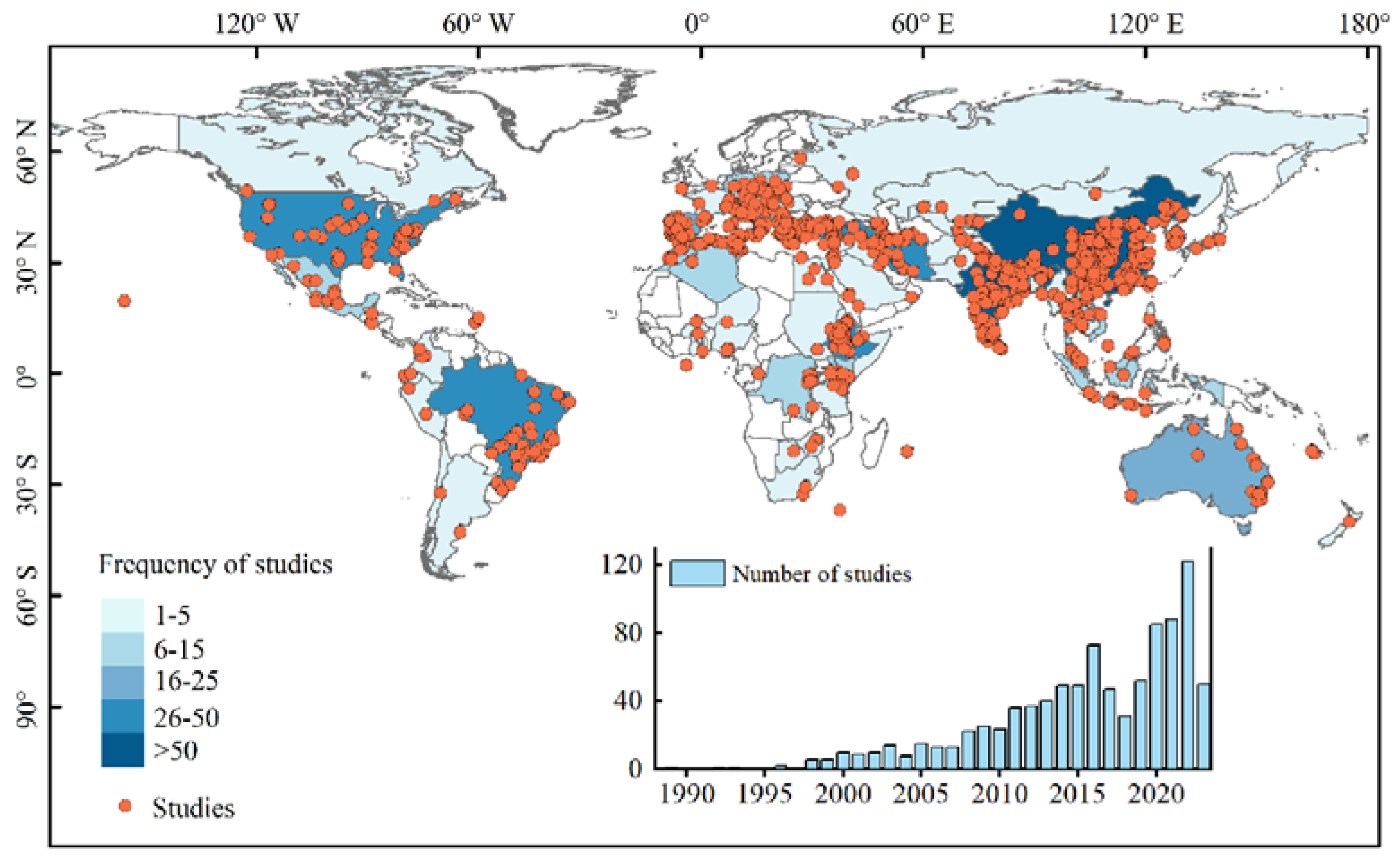
Figure 1. The spatial distribution of the study sites and the number of studies included for analysis for each year.
Remotesensing 15 02868 g001
Figure 2. Boxplots showing the range of C-factor values for main types of land use based on field experiments.
Remotesensing 15 02868 g002
Figure 3. Comparison of measured C-factor values with the literature finding (M2 method).
Remotesensing 15 02868 g003
Figure 4. Regression relationship between NDVI and C-factor value according to the Equations (4)–(12). (a) Linear equations; (b) nonlinear equations; (c) the combined equation based on Equations (11) and (12).
Remotesensing 15 02868 g004
Figure 5. Regression relationship between vegetation coverage (fg, %) and C-factor value according to the Equations (22)–(27).
Remotesensing 15 02868 g005
Figure 6. Changes in the annual number of studies as a function of spatial scales.
Remotesensing 15 02868 g006
Figure 7. Changes in the number of studies using different C-factor methods as a function of (a) the publication year and (b) the study area sizes. M1-6 represent six different categories of the C-factor calculation method.
Remotesensing 15 02868 g007
Figure 8. The mean and standard deviation for C-factor values of each land use.
Remotesensing 15 02868 g008
Table 1. Summary of national and global scale soil erosion assessments using the USLE-type models.
Study AreaC-Factor ValueReferences
EuropeM3: Equation (12)[115,116]
ItalyM3: Equation (12)[59,117]
AustraliaM2[34]
AustraliaM4[118]
South AfricaM2[119]
SpainM2[120]
SlovakiaM2[121]
EuropeM2[122]
South KoreaM2[36]
SpainM6[123]
ChinaM4: Equation (26)[124,125]
EuropeM2[126,127,128]
EuropeM6[1,7,18]
Mediterranean EuropeM3: Equation (12)[68]
AustraliaM2[35]
HungaryM2[38,39]
ItalyM6[114]
GreeceM6[129]
UgandaM3: Equation (12)[130]
KenyaM2[131]
ItalyM6[132]
North KoreaM2[37]
GlobalM2[40,41,133]
Central AsiaM4: Equation (26)[134]
Central AsiaM3: Equation (12)[135]
South AmericaM2[136]
GlobalNo C-factor[137]
GlobalM2[138,139]
GlobalM3: Equation (4)[140]
GlobalM6[17,97]
GlobalM3: Equation (12)[141]
Disclaimer/Publisher’s Note: The statements, opinions and data contained in all publications are solely those of the individual author(s) and contributor(s) and not of MDPI and/or the editor(s). MDPI and/or the editor(s) disclaim responsibility for any injury to people or property resulting from any ideas, methods, instructions or products referred to in the content.