Denoising and Accuracy Evaluation of ICESat-2/ATLAS Photon Data for Nearshore Waters Based on Improved Local Distance Statistics

Abstract

The second-generation spaceborne LiDAR-Ice, Cloud and Land Elevation Satellite-2 (ICESat-2) carries the Advanced Topographic Laser Altimeter System (ATLAS), which can penetrate a certain depth of water, and is one of the important means to obtain the water depth information of nearshore water. However, due to the influence of the atmospheric environment, water quality and color, the system itself and other factors, the photon point cloud introduces survey noise, which restricts the survey accuracy and reliability of nearshore water depth. Therefore, in this study, we presented a photon denoising algorithm for layered processing of submarine surface. Firstly, rough denoising of the original photon data was completed by smoothing filtering. Then, elevation histogram statistics were carried out on the photon data, two peaks of the histogram were fitted by a double Gaussian function, and the intersection of two curves was then taken to separate the water surface and underwater photons. The surface photons were denoised by the DBSCAN clustering algorithm. Then according to the distribution characteristics of underwater signal photons, a single-photon point cloud filtering bathymetric method was proposed based on improved local distance statistics (LDSBM), which was used for fine denoising of underwater point cloud data. Finally, the Gaussian function was used to fit the frequency histogram, and the signal photons were screened to extract the water depth information. In this study, 13 groups of the ATL03 dataset from the Xisha Islands, the St. Thomas and the Acklins Island were used for denoising. The denoising results were compared with the signal photons manually marked and the signal photons extracted by the official built-in method (OM). The experimental results showed that, compared with the official method results of ATL03, the LDSBM had a higher F value (comprehensive evaluation index), with an average of more than 96.70%. In conclusion, the proposed underwater single-photon point cloud filtering bathymetric method was superior to the traditional algorithm and could recover terrain information accurately.

1. Introduction

Nearshore area bathymetric surveys are important for marine surveying and mapping. In the early bathymetry, surveys were completed by manual fieldwork using ship-borne beam bathymeter, which was low in efficiency and unable to meet the dynamic change monitoring needs [1,2]. With the rapid development and progress of remote sensing technology, it had gradually replaced the traditional methods on account of its efficiency and independence of time, climatic conditions and other restrictions. However, this method was extremely limited by the resolution of image data, resulting in low accuracy [3]. On the other hand, Light Detection and Ranging (LiDAR) had been developing rapidly since its emergence and its features, such as high speed, strong anti-interference ability and high accuracy, had brought new breakthroughs to the bathymetric surveys. Nevertheless, this method was neither economical nor feasible for areas in need of periodic monitoring [4].

In 2018, the United States launched the new generation of Ice, Cloud and Land Elevation Satellite-2 (ICESat-2) that carries the Advanced Topographic Laser Altimeter System (ATLAS) with the ability to respond to a single photon that can detect weak signals, greatly improving the detection range and ability. Compared to the Geoscience Laser Altimeter System (GLAS) carried by the first generation of Ice, Cloud and land Elevation Satellite (ICESat), ATLAS was significantly advantageous in low energy, high repetition frequency and narrow pulse, resulting in extremely high accuracy of 3D point cloud data obtained [5]. To be specific, ATLAS laser emits the laser pulses at a frequency of 10 kHz, and can obtain single-photon data with high density and small footprint (the light spot diameter is about 17 m, and the spacing along the same track is about 0.7 m [6]). In addition, ATLAS uses the laser pulse in the green band of 532 nm with a strong penetration ability to a depth at most of 38 m in near-shore waters [7]. Upon emission, the pulse is then divided into six light beams and arrayed into three pairs of light beams. Each pair consists of one strong light beam and one weak light beam, with the light beams about 90 m apart within the beams and the different beams are about 3 km apart. Therefore, ICESat-2/ATLAS has unique advantages and broad application prospects in large-scale lake water level monitoring on account of its small footprint, multi-beam and high-frequency sampling. For example, Xu et al. [8] built a correlation between ICESat-2 laser points for multi-phase Sentinel-2 images on GEE using a linear regression model to generate the shallow water bathymetric chart and verified using LiDAR data, and the results showed RMSE was 1.08 m. Babbel et al. [9] established and tested a standardized method flow of ICESat-2 and satellite image fusion inversion bathymetry, and the RMSE was 0.96 m and 1.54 m upon using Sentinel-2 and Landsat 8 for validation, respectively.

For subsequent use, the currently available product ATL03 in ICESat-2 requires to denoise the data before using photon data due to small photon energy and vulnerability to noise. Neuenschwander et al. [10] proposed a method named Differential, Regressive, and Gaussian Adaptive Nearest Neighbor, (DRAGANN), and according to the feature that the distribution of signal photons distribution was more dense than that of noise photons and was used to generate product ATL08. Chen et al. [11] proposed a method named Adaptive Variable Ellipse Filtering Bathymetric Method (AVEBM) which took the change characteristic of photon density in the water column with the increase of the water depth into account. They used SDB data to verify, and the experiment results showed that the bathymetric accuracy RMSE could reach 0.79 m. However, the AVEBM did not take the neighborhood direction factor into account, leading to discontinuities in the denoising result. Xie et al. [12] had improved the self-adaption Density-Based Spatial Clustering of Applications with Noise (DBSCAN) to extract the signal photon and used the proper outlier detection algorithm to remove the abnormal photon and improved the accuracy. Hsu et al. [13] first obtained the histogram of the elevation distribution of ICESat-2 along the orbit profile, and then used the second-order Gaussian distribution to fit the histogram, so as to separate the sea surface and sea bottom photons. The median filter was used to filter the noise photons iteratively. Finally, the water depth was measured after refraction correction and tide correction. Wang et al. [14] proposed a denoising method based on the adaptive elevation difference threshold (AEDTA). Compared with the clustering method of ordering points to identify the clustering structure (OPTICS), AEDTA extracted more reliable signal photons. Wang et al. [15] utilized interval estimate and modified OPTICS to extract the signal photons, which improved the accuracy of extraction in underwater terrain. Zhang et al. [16] proposed a pre-pruning quadtree isolation (PQI) method with changing threshold, which achieved a 92.71% F1 score.

Since the ICESat-2 laser reaches the water bottom penetrating through the surface, the photon density reflects from the water surface is much greater than that at the bottom. And because of the water quality and environment differences, the water bottom photon conditions in different areas differ. In addition, with the increase of water depth, the density of water bottom photons gradually decreases. There is no obvious rule in the distribution of signal photons so the way to effectively extract water bottom signal photons is the premise of whether ICESat-2/ATLAS data can be used for nearshore bathymetry. In this paper, a water bottom photon filtering bathymetric method based on improved local distance statistics (LDSBM) that was divided into two steps, specifically coarse denoising and fine denoising, to retain as many water bottom signal photons as possible. Taking the islands and reefs of the Xisha Islands in the South China Sea, the St. Thomas and the Acklins Island as the experiment areas, the ways to extract water bottom signal photons were explored and compared to ICESat-2/ATL03 official built-in method (OM) extraction results and manually marked validation photons to verify the accuracy and effectiveness of the algorithm in this paper.

2. Materials and Methods

2.1. Experiment Areas

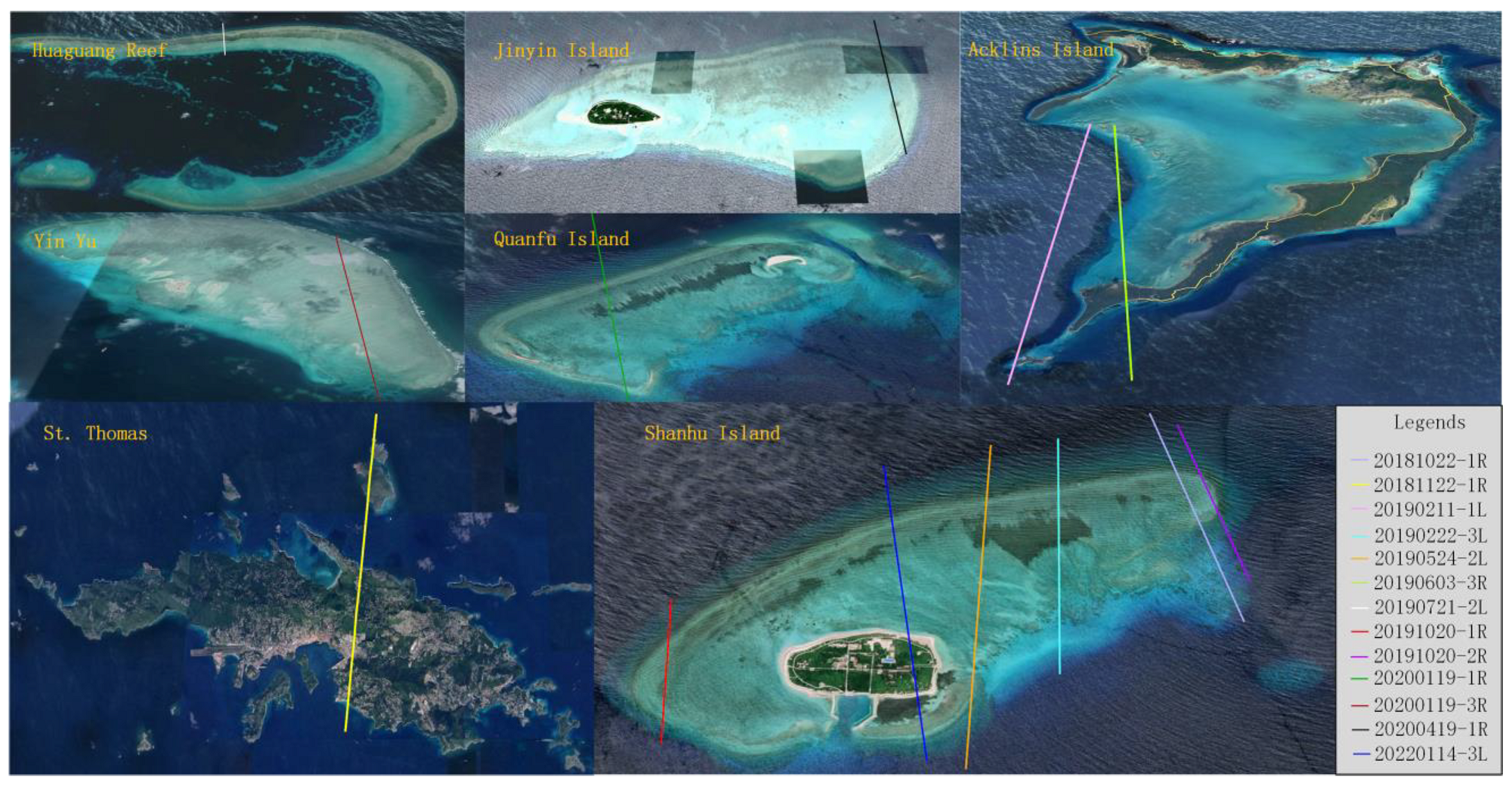
In order to fully verify the accuracy of extracting water bottom photons using the LDSBM, seven islands from three different regions were selected to experiment in this study. As shown in Figure 1a, the first experiment region of this paper is located in Xisha Islands within the South China Sea. The Xisha Islands, with flat terrains and vast sea areas, is the largest archipelago in the South China Sea, consisting of more than 40 islands, islets and reefs. Finally, five islands in the South China Sea (Huaguang Reef, Jinyin Island, Yin Yu, Quanfu Island and Shanhu Island) are selected as the experimental area of this paper. The waters in these areas are clear with low sand contents so the permeability depth of sunlight can at most reach 30 m in such waters, which is suitable for carrying out the experiment of ICESat-2 water bottom denoising and shallow-water optical depth detection. The second region, as Figure 1b shows, is the second-largest island of the US Virgin Islands in the eastern Caribbean Sea. The third region, as Figure 1b shows, is the surrounding waters around the Acklins Island and Long Cay in Southeastern Bahamas.

2.2. ICESat-2 ATL03 Data

The ATL03 photon data track of the experiment areas is shown as Figure 2, and ATL03 data can be downloaded from EarthData (https://search.earthdata.nasa.gov/search, accessed on 10 December 2022). It is the secondary product of the ICESat-2 product and further processes the ATL02 data of the L1 product with the help of accurate pointing and other auxiliary data to generate useful information, including the orbital distance, elevation, longitude, latitude, photon propagation time, and confidence of each photon event. ATL03 dataset contains six beams, including three strong beams and three weak beams whose energy ratio of 4:1 [17], which are labeled as GT1L, GT1R, GT2L, GT2R, GT3L and GT3R, respectively. Photon point cloud data with strong beams usually have high signal-to-noise ratio and sounding ability than with weak beams. In this study, the strong beam data of these thirteen sets of data were used for experiments.

Due to data discontinuity, it was extremely difficult to extract the effective data containing water bottom photons. Therefore, massive land data was ruled out and only the data containing nearshore waters was selected. In the experiment of this paper, thirteen groups of effective ATL03 datasets were eventually selected, with six groups of data crossing Shanhu Island, four groups crossing Huaguang Reef, Jinyin Island, Yin Yu and Quanfu Island, two groups crossing the Acklins Island and one group crossing the St. Thomas respectively.

Table 1. Information of the ATL03 Datasets adopted in this Experiment.

Name of the ATL03 Dataset	Local Acquisition Time	Beam No. Used	Photon Reference
ATL03_20181022073835_03620101_005_01	15:38	GT1R	5,525,850~5,531,700
ATL03_20190222135159_08570207_005_01	21:51	GT3L	611,220~620,235
ATL03_20190524093136_08570307_005_01	17:31	GT2L	9,873,740~9,884,740
ATL03_20190721183749_03620401_005_01	02:37	GT2L	1,169,050~1,171,420
ATL03_20191020141751_03620501_005_01	22:17	GT1R	1,759,220~1,760,930
ATL03_20191020141751_03620501_005_01	22:17	GT2R	1,380,710~1,383,610
ATL03_20200119095733_03620601_005_01	17:57	GT1R	5,316,850~5,328,140
ATL03_20200119095733_03620601_005_01	17:57	GT3R	5,489,800~5,504,320
ATL03_20200419053723_03620701_005_01	13:37	GT1R	11,042,060~11,061,510
ATL03_20220114231625_03621401_005_01	07:20	GT3L	4,621,580~4633590
ATL03_20181122060325_08340107_005_01	14:03	GT1R	1,645,587~1,648,704
ATL03_20190211025118_06820207_005_01	10:51	GT1L	417,804~420,731
ATL03_20190603091752_10100301_005_01	17:17	GT3R	344,236~348,241

lists the thirteen-track dataset information including the name of the ATL03 dataset, local acquisition time, beam num used and photon reference.

3. Research Methods

Because of the characteristic that the photon counting LiDAR system is sensitive to the single photon, it can rapidly collect accurate land data. However, its sensitivity to the single photon will cause various noise effects on the point cloud data [18], which severely affects the subsequent use of ICESat-2 data. Therefore, the key issue to be solved to efficiently and accurately apply the photon counting LiDAR data is the extraction of signal photons.

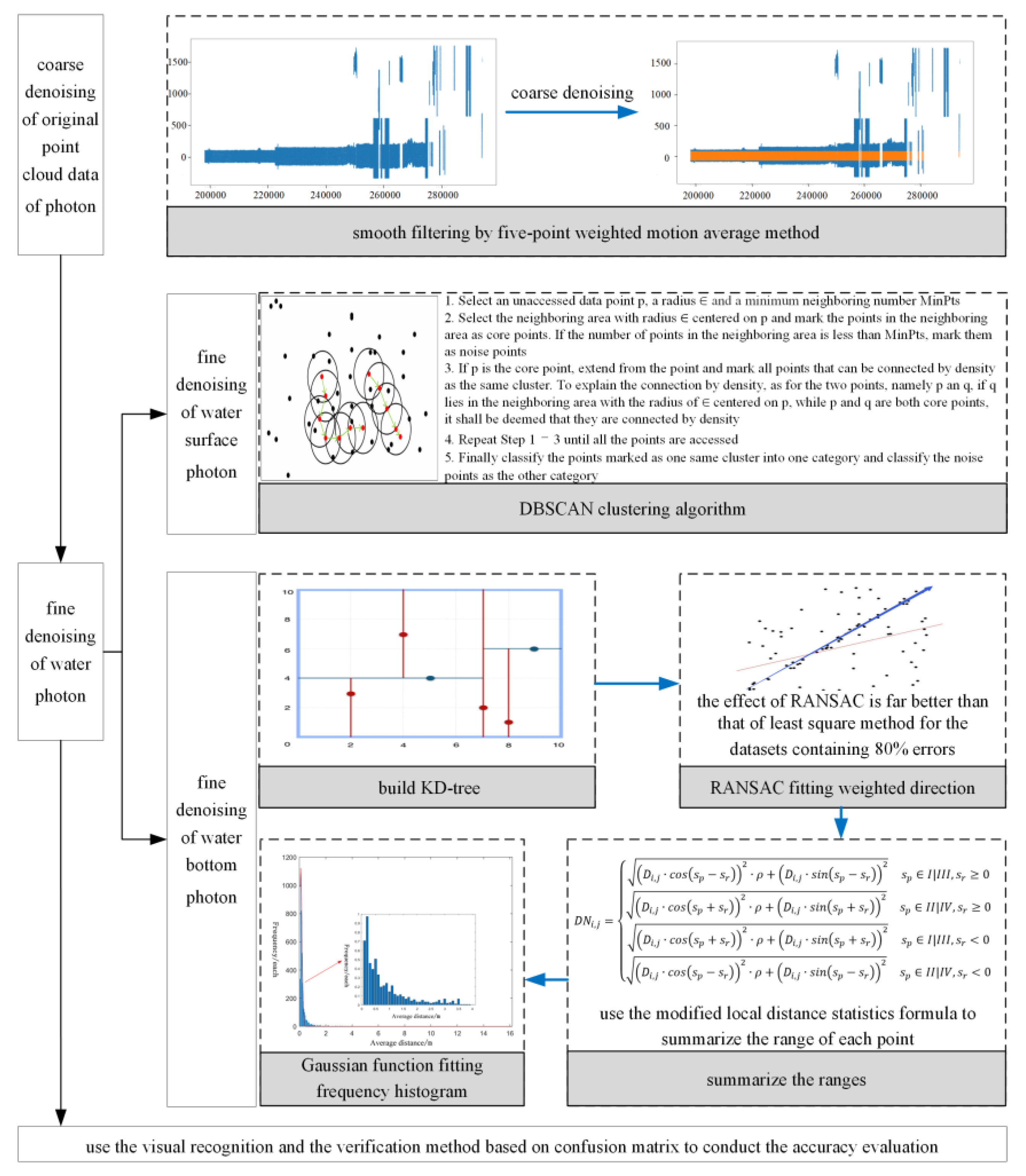
The LDSBM workflow used in this paper is shown in Figure 3. Firstly, the five-point weighted motion average method was used to coarse denoise the original photon data and then divided such data after coarse denoising into water surface photons and water bottom photons for denoising respectively. In addition, the DBSCAN clustering algorithm was used to denoise the water surface photons. In terms of the water bottom photons, the KD tree was firstly built to accelerate the referencing speed and the RANSAC algorithm was next used to fit the weighted direction. Moreover, the local distance statistics formula was improved, weighted in the directions of terrain trend, and then the frequency histogram was conducted with the Gaussian fitting. Accordingly, the thresholds were set to extract the water bottom signal photons. Finally, visual recognition and the verification method based on the confusion matrix conducted the accuracy evaluation.

3.1. Photon Coarse Denoising

In order to reduce data redundancy and improve operational efficiency while reducing the impact of accidental errors, through the elevation histogram statistics of the original single-photon laser point cloud, the motion-weighted average method was adopted to carry out the smooth filtering on the elevation distribution histogram. The filtering formula is shown as below,

$$H_{i,smooth}=a_1\cdot H_{i-2}+a_2\cdot H_{i-1}+a_3\cdot H_i+a_4\cdot H_{i+1}+a_5\cdot H_{i+2}$$

(1)

where $H_{i,smooth}$ refers to the statistical value of the first columnar component of the elevation histogram after smooth filtering. $H_i$ refers to the ith column component in the histogram, where $i\in \left\{1,2,\dots ,N\right\}$. $a_1$, $a_2$, $a_3$, $a_4$ and $a_5$ refer to the five parameters of motion weighted average method, where $a_1=a_5=0.0625$, $a_2=a_4=0.25$ and $a_3=0.375$.

3.2. Photon Fine Denoising

Due to the large difference between the density of water surface photons and water bottom photons, it was required to adopt different denoising methods for the two kinds of photons. The height histogram statistics were carried out for the photon after coarse denoising, and the two peaks of the histogram were fitted with a double Gaussian function. The elevation of the intersection point of the two Gaussian curves was taken as the threshold for the separation of those two kinds of photons. The water surface photons and water bottom photons were denoised separately.

3.2.1. Fine Denoising of Water Surface Photon

In terms of the characteristics of water surface photons, such as large density and concentrated distribution of signal photons, and significant density difference between noise photons and signal photons, the Density-Based Spatial Clustering of Applications with Noise (DBSCAN) clustering method was used for denoising. It was believed in this algorithm that the points connected by density should be classified into one same point set (i.e., cluster) while the outliers not classified should be named as noise points. The DBSCAN clustering algorithm is executed in accordance with the steps provided in Appendix A.

DBSCAN clustering algorithm needs two main parameters, namely the radius (Eps) and the minimum points in the neighboring area (MinPts). The parameter, MinPts, is calculated using the self-adaption formula proposed by Ma et al. [19]. The parameter, Eps, is set with different values according to day and night. The Eps is set to 2 m in the daytime when photon data is dense, and 4 m in the night when photon data is sparse.

$$S{N}_1=\pi R_a{}^2{N}_1/hl$$

(2)

where $N_1$ refers to the total photon number, $h$ refers to the elevation range, and $l$ refers to the range scope along the track.

$$S{N}_2=\pi R_a{}^2{N}_2/h_{2}l$$

(3)

As for the photons with the difference between elevation and minimum elevation not more than 5 m, the expected photon number is of $S{N}_2$ is calculated. In the formula, $N_2$ refers to the photon involved in the calculation and $h_2=5$, and thus the formula to calculate MinPts is shown as below,

$$MinPts=\left(2S{N}_1-S{N}_2\right)/\ln (2S{N}_1/S{N}_2)$$

(4)

If the finally calculated $MinPts$ is less than 3, then $MinPts=3$.

3.2.2. Fine Denoising of Water Bottom Photon

In ICESat-2 single-photon laser point cloud, the density of signal photons in the terrain trend direction, is apparently larger than that in the vertical terrain trend direction. Therefore, in this study, when using local distance statistics as the threshold to distinguish signal photons from noise photons, a weight factor $\rho$ was added in the terrain trend direction to make the photons in the terrain trend direction to be more likely classified as signal photons. The Euclid distance formula is shown as below,

$$D_{i,j}=\sqrt{{\left(x_i-x_j\right)}^2+{\left(y_i-y_j\right)}^2}$$

(5)

where $D_{i,j}$ refers to the Euclid distance between point $i$ and $j$. $i$ and $j$ refer to any two points in the single-photon point cloud. $x_i$ and $x_j$ refer to the distances along track of point $i$ and $j$ in the horizontal direction, respectively. $y_i$ and $y_j$ refer to the elevation values of point $i$ and $j$ in the vertical direction.

The modified distance formula is shown as below,

$$D{N}_{i,j}=\left\{\begin{array}{c}\sqrt{{\left(D_{i,j}·cos\left(s_p-s_r\right)\right)}^2·\rho +{\left(D_{i,j}·sin\left(s_p-s_r\right)\right)}^2}\hspace{1em}{s}_p\in I|III, s_r\ge 0\\ \sqrt{{\left(D_{i,j}·cos\left(s_p+s_r\right)\right)}^2·\rho +{\left(D_{i,j}·sin\left(s_p+s_r\right)\right)}^2}\hspace{1em}{s}_p\in II|IV, s_r\ge 0\\ \sqrt{{\left(D_{i,j}·cos\left(s_p+s_r\right)\right)}^2·\rho +{\left(D_{i,j}·sin\left(s_p+s_r\right)\right)}^2}\hspace{1em}{s}_p\in I|III, s_r<0\\ \sqrt{{\left(D_{i,j}·cos\left(s_p-s_r\right)\right)}^2·\rho +{\left(D_{i,j}·sin\left(s_p-s_r\right)\right)}^2}\hspace{1em}{s}_p\in II|IV, s_r<0\end{array}\right.$$

(6)

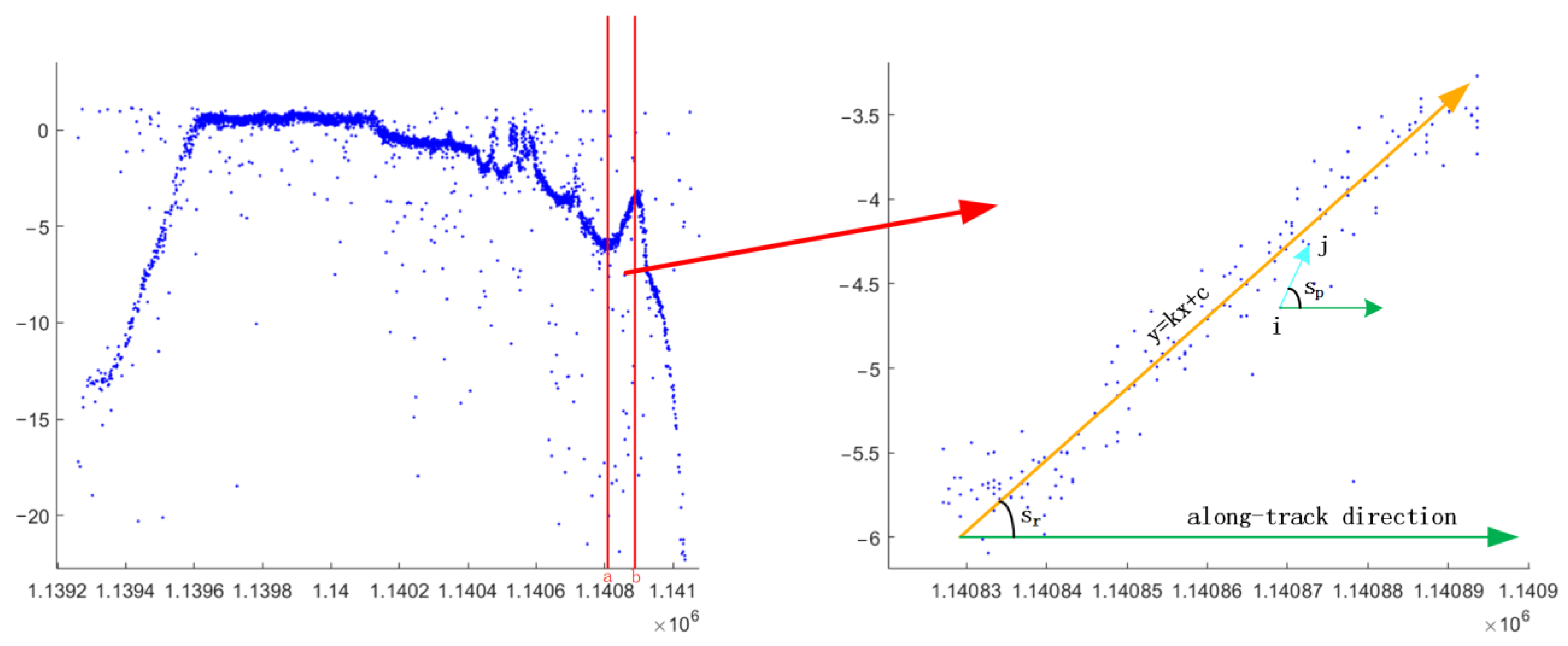
where $D{N}_{i,j}$ refers to the weighted distance value of point $i$ and $j$ in the terrain trend direction. $D_{i,j}$ refers to the Euclid distance between point $i$ and $j$. $\rho$ refers to the weight factor in the terrain trend direction. After the experiment for several times, when $\rho$ is 0.01, the aggregation of point cloud data reaches the peak in the terrain trend direction, and the effect to distinguish noise photon and signal photon is the best. Thus, in this paper, $\rho$ is 0.01. $s_p$ refers to the slope between point $i$ and $j$. $s_r$ refers to the slope of terrain trend direction in the interval where point $i$ and $j$ are located. $\mathit{I}$, $\mathit{II}$, $\mathit{III}$ and $\mathit{IV}$ refer to the quadrants. The definitions of $s_p$ and $s_r$ are shown in Figure 4.

According to the formula above, the steps of ICESat-2 point cloud denoising algorithm are shown as below,

(1)

Build the KD tree indexes for the water bottom photons so as to improve the indexing speed and then search the nearest K points around each point. The KD tree is constructed according to the steps provided in Appendix B.

(2)

Divide the intervals in the along-track direction according to 20 m for the water bottom photons and carry out RANSAC (Random Sample Consensus) straight-line fitting on all the photons in each interval. The basic idea of the RANSAC algorithm is given in Appendix C. The fitted straight line slope is the slope of the terrain trend direction in this interval $s_r$ and it is weighted in this direction.

(3)

According to the modified distance formula, the average values of the local distance sum of the nearest K points from each point $D{M}_i$ are counted.

$$D{M}_i={{\displaystyle \sum }}_{n=1}^{K}D{N}_{i,j}/K$$

(7)

(4)

Because there are many fine sands in the water bottom area near the sea surface, ATL03 single-photon data will penetrate to the bottom through fine sands in this area, with obvious layering. Thus, it is required to remove the water bottom photons in shallow water areas. According to the elevation of water bottom point cloud data, the distribution histogram is built to divide the point cloud data into N intervals according to the equal elevation interval and count the total number of photons in each elevation interval. The average value of the elevation histogram is calculated and then look through the histogram to find the most elevation sections continuously larger than the average value for DBSCAN clustering denoising.

(5)

Conduct the frequency statistics on the average distance $D{M}_i$, and produce the frequency histogram $h_{DM}$ with 0.1 as the spacing. Conduct the Gaussian curve fitting on $h_{DM}$, and search the final elevation section $n$ whose frequency is lower than $\mu /2$ with the peak value of $h_{DM}$ as the average value $\mu$ of the Gaussian curve based on the Gaussian curve half-width and full-height theorem. $sigma$ refers to the difference between the abscissa of the elevation section $n+1$ and the average value $\mu$. The average distance threshold is set to be the sum of the average value $\mu$ and t-fold $sigma$. Those whose average distance is larger than the threshold shall be noise photon while the rest shall be water bottom signal photons.

$$sigma=x_{n+1}-\mu$$

(8)

where $sigma$ refers to the variance of the Gaussian curve. $x_{n+1}$ refers to the abscissa corresponding to the $n+1$ th elevation section. $\mu$ refers to the average value of the Gaussian curve.

3.3. Accuracy Evaluation

Referring to the remote sensing image classification accuracy evaluation method [20], the visual recognition and verification method based on the confusion matrix were used to evaluate the signal photons extracted by the denoising method in this paper. In the visual recognition, whether there was an obvious classification error between water bottom signal photons and noise photons was mainly manually judged. The verification method based on the confusion matrix referred to the evaluation by statistical comparison of attribute information of the labeled water body signal photons and signal photons extracted by the LDSBM using manually labeled water signal photons.

Three quantitative indicators were used to evaluate the denoising accuracy of the LDSBM, namely the recall rate ($R$), precision ($P$) and comprehensive evaluation index ($F$), where $R$ refers to the proportion of the total number of signal photons correctly determined to the original photons. $P$ refers to the ratio of the total number of signal photons correctly determined to the extracted signal photons. $F$ refers to the harmonized average of recall rate and accuracy rate.

$$R=TP/\left(TP+FN\right)$$

(9)

$$P=TP/\left(TP+FP\right)$$

(10)

$$F=2PR/\left(P+R\right)$$

(11)

where $TP$ refers to the total number of photons that the signal photons extracted by the LDSBM and the manually labeled signal photons were all effective water body signal photons. $TN$ refers to the total number of photons that were judged as noise by the LDSBM and by artificial labeling. $FN$ refers to the total number of photons that were judged as noise by the LDSBM and are judged as signals by artificial labelling. $FP$ refers to the total number of photons that were judged as signals by the LDSBM and were judged as noise by manually marked.

4. Data Processing and Results

4.1. Point Cloud Denoising Experiment

In order to understand more clearly how the LDSBM algorithm was conducted with photon separation and threshold selection, and ATL03_20190222135159_08570207_005_01 data is used therein as the example in this section to demonstrate the specific workflow.

4.1.1. Threshold Selection for Photon Separation

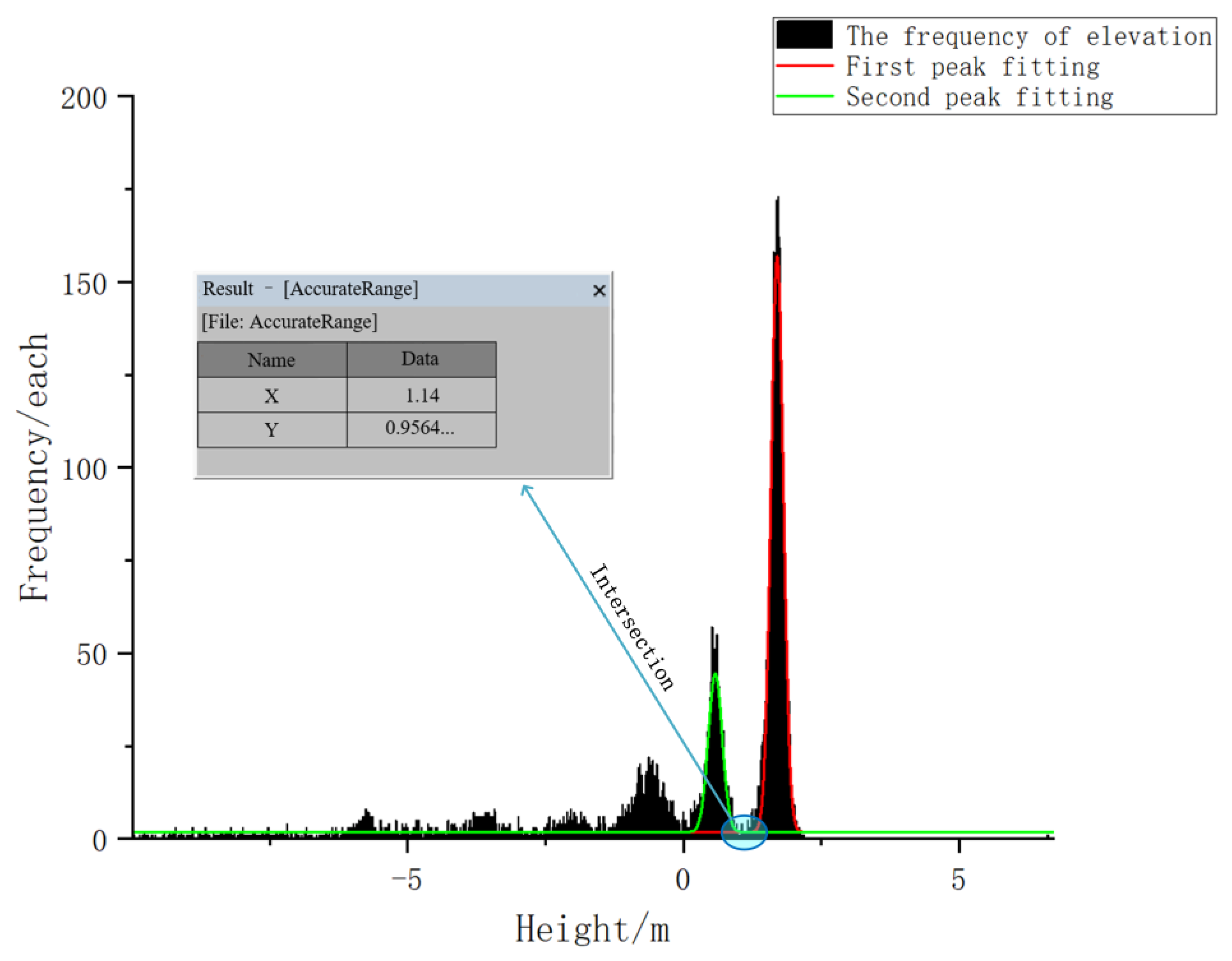
The GT3L beam data of ATL03_20190222135159_08570207_005_01 was screened to intercept the terrain range containing nearshore waters and separate the surface and bottom photons in this part. All photon elevations were statistically generated to generate the frequency histogram, which was fitted by the Gaussian curve twice, and the intersection point of the two curves was taken as the threshold of separation. In this paper, Origin software (https://www.originlab.com/, accessed on 10 December 2022) was used for the Gaussian curve fitting to complete the above operations. The point of intersection of two Gaussian curves is shown in Figure 5.

4.1.2. Threshold Selection for Gaussian Curve Fitting

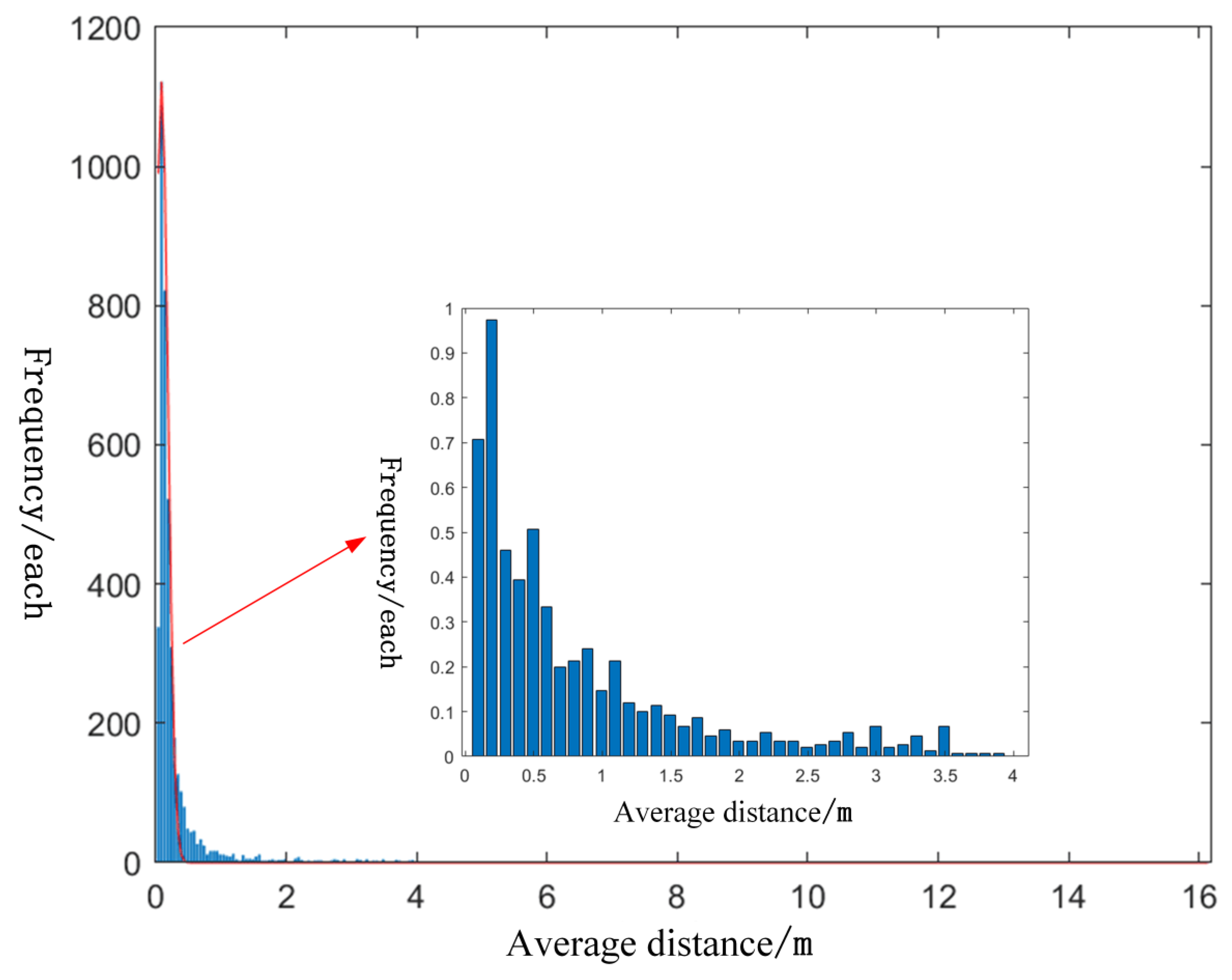
This part explains how to set thresholds to classify photons after counting the improved local distances. K was set as 8 and the intervals were divided equally by 20 m, and the frequency histogram of the average distance $D{M}_i$ is shown as Figure 6. In the figure, the frequency ordinate with an average distance of less than 4 m is scaled down to facilitate the finding of distribution characteristics of frequency. The frequency histogram was generated at an interval of 0.1 m, and the Gaussian curve was used to fit the frequency histogram. With the average distance of 0.0883 m corresponding to the peak value of the histogram as the mean value, the final elevation section whose frequency was below 0.04415 was searched, and the difference between the average distance and mean value of the next elevation section of the aforesaid elevation section was taken as the standard deviation. Thus, the standard deviation of the Gaussian function was 0.1 m and the average distance threshold was the sum of the mean value and t-fold standard deviation. The criterion for setting the parameter t was to retain the signal photon as many as possible. According to the selected ATL03 data, when the parameter t was set as 7, the extraction effect of the signal photons was the best, at which the threshold was 0.7883 m.

4.2. Denoising Results

ATL03 dataset contains not only the exact longitude, latitude and elevation values of photons, but also an important parameter signal_conf_ph. It refers to the confidence parameter for photon classification in the heights dataset. There are five values of each photon in the signal_conf_ph array, which are classified into five categories (land, sea, sea ice, land ice and inland water). The confidence value ranges from 0 to 4. The higher the value is, the more accurate the classification is. Therefore, the photon data of signal_conf_ph ≥ 3 [21,22] was selected in this paper as the signal photon background classification threshold.

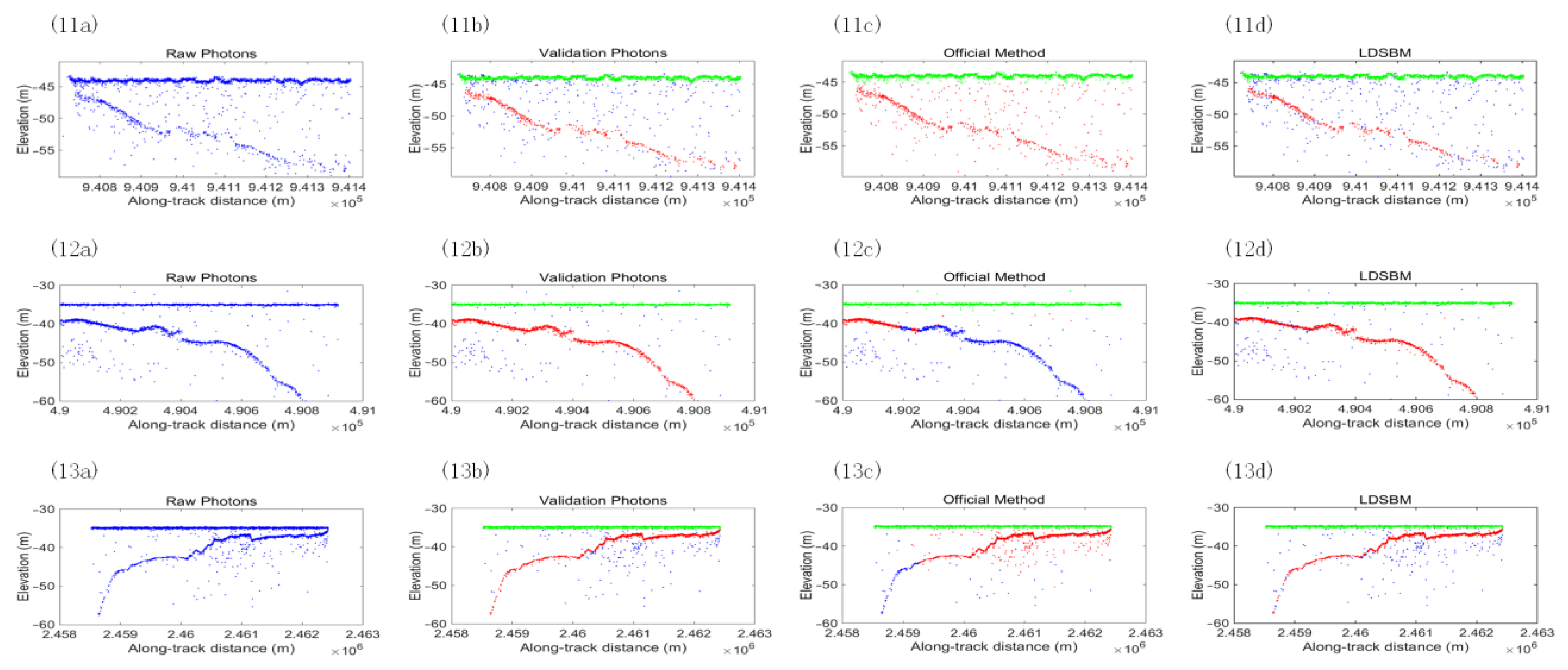
The first column data is the water bottom original photons, the second column data is manually marked signal photons, the third column data is signal photons extracted by the official built-in denoising method and the fourth column data is the signal photons extracted by the LDSBM are displayed in Figure 7 and Figure 8, respectively. In the figure, green dots are water surface photons, red dots are signal photons extracted by various methods, and blue dots are original photons. It can be seen from the figure that the official built-in denoising method can extract flat shallow signal photons. However, with the constant change of water depth, it is difficult to extract signal photons from the water bottom by official method, and it may even identify the noise photons as signal photons, which severely affects the data use. The LDSBM is weighted in the terrain trend direction, making the photons in the terrain trend direction more aggregated and more inclined to be identified as signal photons. The LDSBM can accurately extract the signal photons at different depths. In the thirteen groups of data, the shallow photon data can be correctly extracted by both the LDSBM and the OM. As for deep data, the LDSBM can extract the signal photons more comprehensively and accurately by the LDSBM compared to the official method.

In Figure 7 and Figure 8, the order from 1 to 13 is shown according to the sequence of ATL03 datasets in Table 1. In terms of the data of groups 2, 3, 6, 7, 8, 9 and 10, because there are many fine sands in the shallow water and the soil is loose, the 532 nm laser will penetrate into the deeper water through the fine sand gaps, forming obvious layering, and the area within this range needs to be processed according to step (4) of the LDSBM. Among the seven groups of data, the official method is unable to process the layering data (which is defined as two layers in this paper, including the upper layer data of real terrain and the lower layer data of virtual terrain), the lower layer noise photons are identified as signal photons by mistake. Meanwhile, the LDSBM conducts special processing on the layering data, and the lower layer photons are identified as noise photons. However, in the data of groups 3, 8 and 10, the LDSBM is faced with the problem of determining a small number of signal photons as noise photons for the part with the lowest elevation in the upper layer data, ensuring that the signal photons extracted by the LDSBM are consistent with the manually labeled signal photons to the maximum extent. The existence of some water surface photons in the data of groups 1, 2, 3, 7, 9, 10 and 13, is because when separating water surface and water bottom photons, some photons are at the junction of the threshold and are not completely distinguished. However, such existence does not affect the denoising processing of water bottom photons.

5. Discussion

5.1. Global Precision Discussion

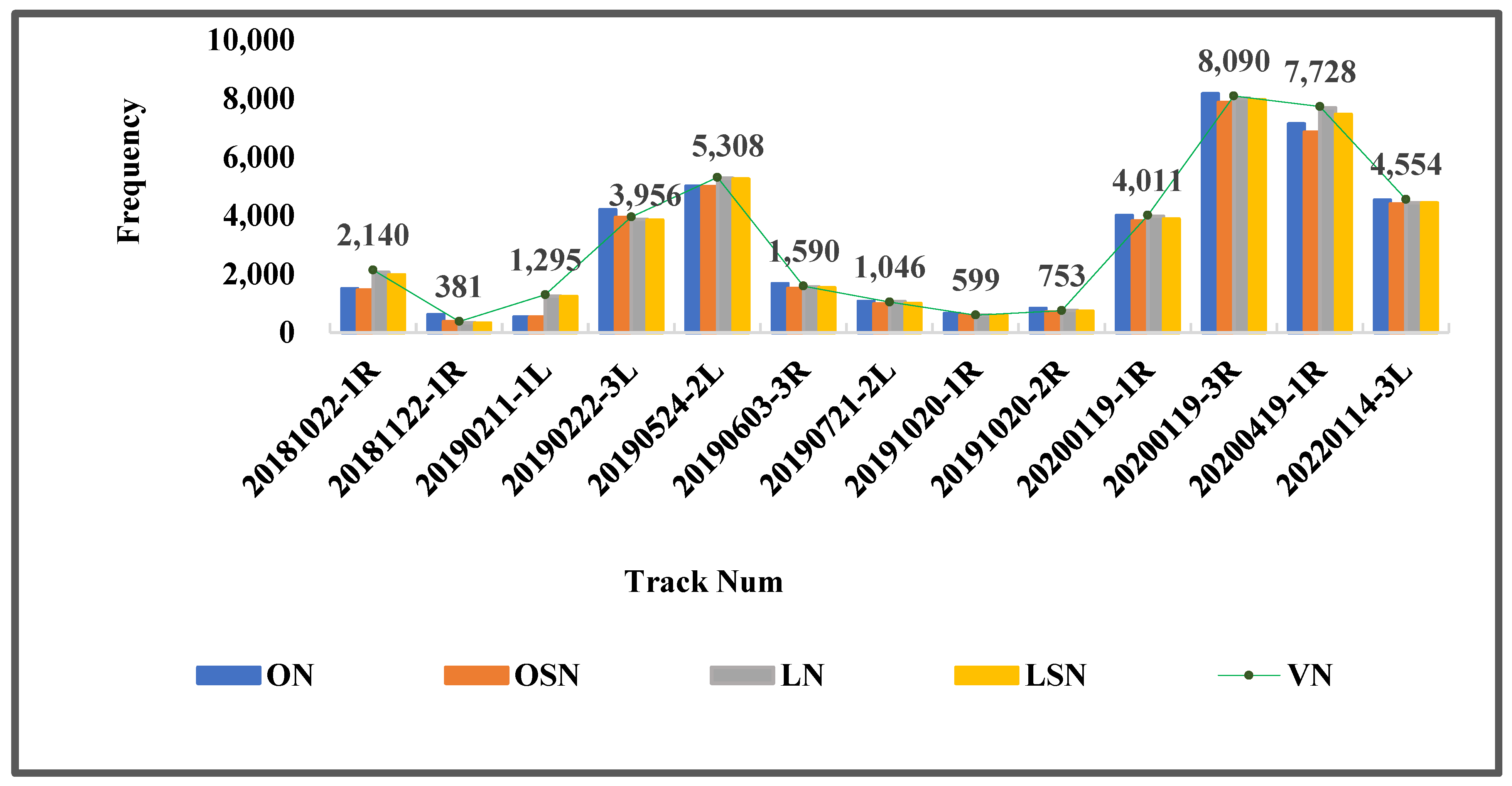
In order to evaluate the performance of the LDSBM in extracting water bottom signal photons, qualitative and quantitative methods are used to evaluate the denoising results of experimental data. In the qualitative evaluation, visual recognition is mainly adopted to subjectively determine whether the signal photons are obviously classified by error. In the quantitative evaluation, the quantitative indicators, including the precision ($P$), the recall rate ($R$) and the comprehensive evaluation index ($F$), are used, leading to more intuitive and accurate evaluation results. The visual recognition can easily and intuitively identify large differences, but is unable to measure the tiny differences. And consequently, F needs to be introduced for quantitative analysis (

Table 2. Statistical information of water bottom signal photon extraction.

ATL03	ON	OSN	LN	LSN	VN	RN
20181022-1R	1505	1456	2064	1974	2140	3045
20181122-1R	612	381	338	330	381	622
20190211-1L	542	532	1248	1236	1295	1408
20190222-3L	4202	3945	3876	3845	3956	4242
20190524-2L	5007	4987	5273	5249	5308	6018
20190603-3R	1671	1506	1560	1537	1590	1784
20190721-2L	1064	986	1061	998	1046	1199
20191020-1R	653	593	601	581	599	665
20191020-2R	826	708	754	728	753	937
20200119-1R	4000	3818	3973	3883	4011	4948
20200119-3R	8164	7867	8015	7957	8090	8850
20200419-1R	7134	6851	7682	7461	7728	10,650
20220114-3L	4531	4401	4437	4433	4554	5122

). The photons extracted by the official built-in denoising method and the LDSBM are mapped to manually labeled signal photons and the number of effective signal photons extracted by the two methods, respectively, is obtained. The number of manually labeled signal photons (VN) refers to the number of photons that are manually identified as the category of signal photons. The total number of signal photons extracted by the official built-in denoising method (ON) refers to the number of photons whose confidence is greater than 2. The number of effective signal photons extracted by the official built-in denoising method (OSN) refers to the number of photons in the intersection of the ON and the VN. The total number of signal photons extracted by the LDSBM (LN) refers to the number of photons that are judged as signal photons in the LDSBM algorithm. The number of effective signal photons extracted by the LDSBM (LSN) refers to the number of photons in the intersection of the LN and the VN. The number of original photons (RN) refers to the total number of photons in the original data.

It can be seen from Figure 9 that, in terms of the data of groups 20181022-1R, 20190211-1L, 20190524-2L and 20200419-1R, LN is more than the ON. In terms of other data, the LN is less than the ON. In terms of the data of the aforesaid four groups, the OSN is far less than the LSN. In terms of the data of the remaining nine groups, the OSN is also less than the LSN, proving that the LDSBM extracts signal photons better than the official built-in method. In addition, the LSN is close to the VN in each group, indicating that the signal photons extracted by the LDSBM are very close to the results of manual labeling with extremely few misextracted photons.

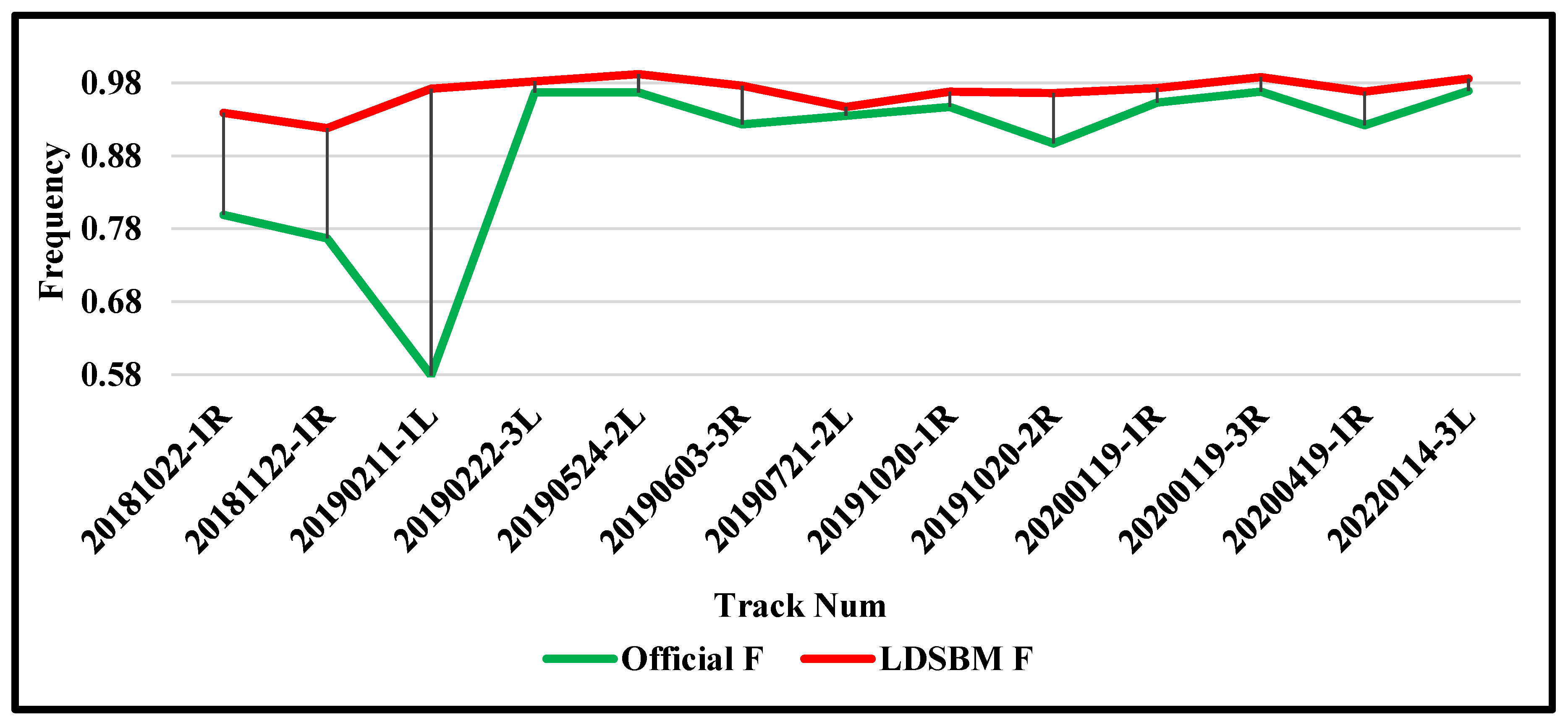
Through further quantitative analysis (

Table 3. Accuracy evaluation information of water bottom signal photons.

ATL03	OM			LDSBM
	R	P	F	R	P	F
20181022-1R	0.680	0.967	0.799	0.922	0.956	0.939
20181122-1R	1.000	0.623	0.767	0.866	0.976	0.918
20190211-1L	0.411	0.982	0.579	0.954	0.990	0.972
20190222-3L	0.997	0.939	0.967	0.972	0.992	0.982
20190524-2L	0.940	0.996	0.967	0.989	0.995	0.992
20190603-3R	0.947	0.901	0.923	0.967	0.985	0.976
20190721-2L	0.943	0.927	0.935	0.954	0.941	0.947
20191020-1R	0.990	0.908	0.947	0.970	0.967	0.968
20191020-2R	0.940	0.857	0.897	0.967	0.966	0.966
20200119-1R	0.952	0.955	0.953	0.968	0.977	0.973
20200119-3R	0.972	0.964	0.968	0.984	0.993	0.988
20200419-1R	0.887	0.960	0.922	0.965	0.971	0.968
20220114-3L	0.972	0.971	0.969	0.973	0.999	0.986

), the water bottom signal photon extracted by the LDSBM can obtain a higher F value with an average of 96.73%. The F value of OM is 89.18%, which is improved by about 7.55%. As for 20181022-1R, 20181122-1R and 20190721-2L, the effect of F after the LDSBM denoising is relatively worse. 20181022-1R is worse in effect because the underwater terrain is complex and the noise photon in some parts are relatively dense and are easy to be extracted by mistake. 20181122-1R and 20190721-2L are worse in denoising effect because the total number of photons in this group of data is very small with a low signal-to-noise ratio and difficulty in denoising. The three groups of data with the largest difference between the official algorithm and the LDSBM harmonic average are 20181022-1R, 20181122-1R and 20190211-1L. It can be seen from Figure 7 and Figure 8 that the official algorithm cannot extract the photon in the relatively deep water bottom, resulting in insufficient extraction accuracy and incomplete information. On the other hand, there is the most similar F value by the official algorithm and the LDSBM algorithm in group 20190721-2L because the data is high in signal-to-noise ratio. Most photons are concentrated within −10 m and the noise photons are distributed uniformly and sparsely, showing a significant difference in density compared to signal photons and easy extraction. The signal photons are extracted from the original photons in the nearshore waters to the maximum, and the noise photons are removed. Compared to the local distance statistics, this algorithm solves the problem that photons are only more concentrated along the track direction, and cannot be applied to complex terrain environment areas. Under good data conditions, the official built-in denoising algorithm can effectively extract signal photons, but may easily classify the noise photons with a large density as signal photons by mistake. The algorithm in this paper was weighted in the terrain trend direction, successfully distinguishing the noise photons and signal photons with high outlier density. This algorithm can process the data with different signal-to-noise ratios, and the experiment results prove the stability and accuracy of signal photons extracted by this algorithm and the F value of most of the study areas can finally reach 95% (Figure 10) and above.

5.2. Delamination Precision Discussion

In this paper, the water bottom signal photons were divided into two categories for evaluation, namely the shallow photons (water bottom photons whose elevation difference from the surface photons are greater than −2.5 m) and the deep photons (water bottom photons whose elevation difference from the surface photons are smaller than −2.5 m). In Figure 11a, the F value of shallow photons by the LDSBM is higher than that by the OM. However, there is only a greater difference in the data of groups 1, 9 and 12, as the shallow photon are relatively aggregated with slightly smaller density than the water surface photons but far larger density than the water bottom photons, resulting in them being extracted easily. Moreover, the signal photons of the official algorithm adopted in this paper are photons whose confidence is greater than or equal to 3. In the official file, 3 is the medium confidence and the official algorithm extracts more photons but erroneously identifies more noise photons as the signal photons. It can be seen from Figure 7 and Figure 8 that the misidentification is heavier. In Figure 11b, most F values of deep photons by the LDSBM are far higher than the F values by the OM. Even as for the data of groups 5, 7 and 12, the official algorithm cannot extract the signal photon, because the density difference between signal photon and noise photon in the three groups of deep photon data is small with scatter distribution and difficult extraction. In conclusion, in the water bottom photon, the LDSBM algorithm is better than the OM algorithm and can accurately restore the terrain information.

6. Conclusions

Targeting at the difficulty in photon extraction from LiDAR signal of spaceborne photon technology, a filtering bathymetric method based on improved local distance statistics to extract the signal photon in nearshore waters was proposed in this paper, namely LDSBM. Using ATL03 data crossing the South China Sea, the St. Thomas and the Acklins Island for the experiment, a relatively good extraction effect of water bottom signal photons was achieved. In this paper, the LDSBM algorithm was used for water bottom signal photons extraction, which increased the weight of water bottom photons in the terrain trend direction to improve the point cloud aggregation in the terrain trend direction and improved the extraction accuracy of signal photons in waters with complex water bottom terrains. In the denoising experiment process, combined with the actual distribution characteristics of point cloud data, some empirical values were reasonably adopted and the setting of such parameter values needed to be reasonably made according to the characteristics of selected data. Considering that the water quality in most shallow water areas is turbid, ICESat-2 data cannot detect the water bottom terrains penetrating through the surface well, so the adaptability of this algorithm remains to be further studied, which is also the difficulty in spaceborne photon counting radar sounding at present. Meanwhile, when fitting the Gaussian curve with the distribution histogram, the parameters cannot be set the automatically, requiring further improvement in automation of this algorithm.

References

1. Westaway, R.M.; Lane, S.N.; Hicks, D.M. Remote sensing of clear-water, shallow, gravel-bed rivers using digital photogrammetry. Photogramm. Eng. Remote Sens. 2001, 67, 1271–1282. [Google Scholar]
2. Brown, C.J.; Beaudoin, J.; Brissette, M.; Gazzola, V. Multispectral multibeam echo sounder backscatter as a tool for improved seafloor characterization. Geosciences 2019, 9, 126. [Google Scholar] [CrossRef]
3. Hua, L.W.; Bi, Y.L.; Hao, L. The research of artificial shoreline extraction based on airborne LIDAR data. J. Phys. Conf. Ser. 2021, 2006, 012048. [Google Scholar] [CrossRef]
4. Paravolidakis, V.; Ragia, L.; Moirogiorgou, K.; Zervakis, M.E. Automatic coastline extraction using edge detection and optimization procedures. Geosciences 2018, 8, 407. [Google Scholar] [CrossRef]
5. Xu, N.; Ma, Y.; Zhang, W.; Wang, X.H.; Yang, F.; Su, D. Monitoring Annual Changes of Lake Water Levels and Volumes over 1984–2018 Using Landsat Imagery and ICESat-2 Data. Remote Sens. 2020, 12, 4004. [Google Scholar] [CrossRef]
6. Abdalati, W.; Zwally, H.J.; Bindschadler, R.; Csatho, B.; Farrell, S.L.; Fricker, H.A.; Harding, D.; Kwok, R.; Lefsky, M.; Markus, T.; et al. The ICESat-2 laser altimetry mission. Proc. IEEE 2010, 98, 735–751. [Google Scholar] [CrossRef]
7. Parrish, C.E.; Magruder, L.A.; Neuenschwander, A.L.; Forfinski-Sarkozi, N.; Alonzo, M.; Jasinski, M. Validation of ICESat-2 ATLAS bathymetry and analysis of ATLAS’s bathymetric mapping performance. Remote Sens. 2019, 11, 1634. [Google Scholar] [CrossRef]
8. Xu, N.; Ma, X.; Ma, Y.; Zhao, P.; Yang, J.; Wang, X.H. Deriving Highly Accurate Shallow Water Bathymetry from Sentinel-2 and ICESat-2 Datasets by a Multitemporal Stacking Method. IEEE J. Sel. Top. Appl. Earth Obs. Remote Sens. 2021, 14, 6677–6685. [Google Scholar] [CrossRef]
9. Babbel, B.J.; Parrish, C.E.; Magruder, L.A. ICESat-2 elevation retrievals in support of satellite-derived bathymetry for global science applications. Geophys. Res. Lett. 2021, 48, e2020GL090629. [Google Scholar] [CrossRef]
10. Neuenschwander, A.; Pitts, K. The ATL08 land and vegetation product for the ICESat-2 Mission. Remote Sens. Environ. 2019, 221, 247–259. [Google Scholar] [CrossRef]
11. Chen, Y.; Le, Y.; Zhang, D.; Wang, Y.; Qiu, Z.; Wang, L. A photon-counting LiDAR bathymetric method based on adaptive variable ellipse filtering. Remote Sens. Environ. 2021, 256, 112326. [Google Scholar] [CrossRef]
12. Xie, C.; Chen, P.; Pan, D.; Zhong, C.; Zhang, Z. Improved Filtering of ICESat-2 Lidar Data for Nearshore Bathymetry Estimation Using Sentinel-2 Imagery. Remote Sens. 2021, 13, 4303. [Google Scholar] [CrossRef]
13. Hsu, H.-J.; Huang, C.-Y.; Jasinski, M.; Li, Y.; Gao, H.; Yamanokuchi, T.; Wang, C.-G.; Chang, T.-M.; Ren, H.; Kuo, C.-Y.; et al. A semi-empirical scheme for bathymetric mapping in shallow water by ICESat-2 and Sentinel-2: A case study in the South China Sea. ISPRS J. Photogramm. Remote Sens. 2021, 178, 1–19. [Google Scholar] [CrossRef]
14. Wang, B.; Ma, Y.; Zhang, J.; Zhang, H.; Zhu, H.; Leng, Z.; Zhang, X.; Cui, A. A noise removal algorithm based on adaptive elevation difference thresholding for ICESat-2 photon-counting data. Int. J. Appl. Earth Obs. Geoinf. 2023, 117, 103207. [Google Scholar] [CrossRef]
15. Wang, Z.; Xi, X.; Nie, S.; Wang, C. Bathymetric Method of Nearshore Based on ICESat-2/ATLAS Data—A Case Study of the Islands and Reefs in The South China Sea. In Proceedings of the IGARSS 2022-2022 IEEE International Geoscience and Remote Sensing Symposium, Kuala Lumpur, Malaysia, 17–22 July 2022; IEEE: Piscataway Township, NJ, USA, 2022; pp. 2868–2871. [Google Scholar]
16. Zhang, G.; Xing, S.; Xu, Q.; Li, P.; Wang, D. A Pre-Pruning Quadtree Isolation Method with Changing Threshold for ICESat-2 Bathymetric Photon Extraction. Remote Sens. 2023, 15, 1629. [Google Scholar] [CrossRef]
17. Magruder, L.; Brunt, K.; Neumann, T.; Klotz, B.; Alonzo, M. Passive ground-based optical techniques for monitoring the on-orbit ICESat-2 altimeter geolocation and footprint diameter. Earth Space Sci. 2021, 8, e2020EA001414. [Google Scholar] [CrossRef]
18. Le, Y.; Hu, M.; Chen, Y.; Yan, Q.; Zhang, D.; Li, S.; Zhang, X.; Wang, L. Investigating the Shallow-Water Bathymetric Capability of Zhuhai-1 Spaceborne Hyperspectral Images Based on ICESat-2 Data and Empirical Approaches: A Case Study in the South China Sea. Remote Sens. 2022, 14, 3406. [Google Scholar] [CrossRef]
19. Ma, Y.; Xu, N.; Liu, Z.; Yang, B.; Yang, F.; Wang, X.H.; Li, S. Satellite-derived bathymetry using the ICESat-2 lidar and Sentinel-2 imagery datasets. Remote Sens. Environ. 2020, 250, 112047. [Google Scholar] [CrossRef]
20. Koblinsky, C.J.; Clarke, R.T.; Brenner, A.C.; Frey, H. Measurement of river level variations with satellite altimetry. Water Resour. Res. 1993, 29, 1839–1848. [Google Scholar] [CrossRef]
21. Ye, J.; Qiang, Y.; Zhang, R.; Liu, X.; Deng, Y.; Zhang, J. High-precision digital surface model extraction from satellite stereo images fused with ICESat-2 data. Remote Sens. 2021, 14, 142. [Google Scholar] [CrossRef]
22. Li, R.; Li, H.; Hao, T.; Qiao, G.; Cui, H.; He, Y.; Hai, G.; Xie, H.; Cheng, Y.; Li, B. Assessment of ICESat-2 ice surface elevations over the Chinese Antarctic Research Expedition (CHINARE) route, East Antarctica, based on coordinated multi-sensor observations. Cryosphere 2021, 15, 3083–3099. [Google Scholar] [CrossRef]
Figure 1. Geographic Location of the Experiment Areas. (The locations of the Xisha Islands are shown in (a), and the locations of the Acklins Island and the St. Thomas are shown in (b).
Remotesensing 15 02828 g001
Figure 2. Laser Track Map of the Experiment Areas.
Remotesensing 15 02828 g002
Figure 3. Method Flow Chart.
Remotesensing 15 02828 g003
Figure 4. Slope definition diagram. The point i and point j are located in the [a, b] range, the yellow arrow refers to the straight line direction obtained by using the RANSAC method to fit all points in the [a, b] range, the green arrow refers to the along-track direction, and the blue arrow refers to the direction from point i to point j. s r is the angle between the yellow arrow and the green arrow, and s p is the angle between the blue arrow and the green arrow.
Remotesensing 15 02828 g004
Figure 5. Gaussian curve fitting.
Remotesensing 15 02828 g005
Figure 6. Frequency histogram of average distance of each point.
Remotesensing 15 02828 g006
Figure 7. Comparison of fine denoising results of the Xisha Islands (the green points refer to water surface photons, the red points refer to signal photons extracted by all methods, blue points refer to the original photons).
Remotesensing 15 02828 g007
Figure 8. Comparison of fine denoising results of the St. Thomas and the Acklins Island (the green points refer to water surface photons, the red points refer to signal photons extracted by all methods, blue points refer to the original photons).
Remotesensing 15 02828 g008
Figure 9. Statistical information chart.
Remotesensing 15 02828 g009
Figure 10. Accuracy evaluation chart.
Remotesensing 15 02828 g010
Figure 11. Laying accuracy evaluation chart (comparison of shallow signal photon extraction is shown as (a) and comparison of deep signal photon extraction is shown as (b)).
Remotesensing 15 02828 g011