A Novel Fast Sparse Bayesian Learning STAP Algorithm for Conformal Array Radar

Abstract

Space-time adaptive processing (STAP) is an important method of clutter suppression that requires adequate training samples. For an airborne conformal array radar, conventional STAP methods do not have enough training samples to acquire good performance due to the range dependent clutter caused by geometry and the problem of polarization. Sparse-recovery-based STAP (SR-STAP) methods have garnered significant attention in the past few decades because they only require a small number of training samples. Sparse Bayesian Learning (SBL) methods have seen increasing amounts of development due to its robust, self-regularizing nature and because it is not sensitive to user parameters, but it converges slowly. In this paper, a novel fast SBL (NFSBL) method is put forward to increase the rate of convergence. To minimize the SBL penalty function, the proposed method introduces the conjugate function to construct a surrogate function. Additional solution sparsity will be achieved through iteratively minimizing the surrogate function. Then, from the proposed method, we could obtain a more accurate clutter plus noise covariance matrix. Numerical simulation results express that this method could acquire better performance of STAP and improvement in convergence and computational complexity for a conformal array.

1. Introduction

Conformal array radar has attracted extensive attention because of the advantages which contain the underlying larger effective aperture, minimum payload weight, rise scanning range without cumbersome mechanical couplings and avoiding signal modulation from rotary antenna [1].

Space-time adaptive processing (STAP) is a meaningful method because of its excellent clutter suppression performance [2]. The optimum weight vector aims to maximize the output signal-interference-noise-ratio (SINR) [3]. Usually, the clutter plus noise covariance matrix (CNCM) should be obtained by using the training samples with the adjacent to range cell under test (CUT) to estimate [4]. The Reed–Mallett–Brennan rule (RMB) [5] shows that the training samples must fulfill these conditions to maintain a 3 dB output SINR loss: (a) it should be independent and identically distributed (IID); (b) it is required to have no target; (c) the number is required to be more than twice the degrees of freedom. However, in the complex structures, such as conformal arrays, there is nonlinearity and range-dependence between the Doppler frequencies and spatial frequencies. Meanwhile, clutter has no stationarity over the range [6]. For conformal arrays, it is more difficult to acquire the needed IID training samples.

In order to deal with influence caused by range dependence, many methods based on compensation have been proposed. The angle-Doppler compensation method (ADC) [7] deterministically aligns maximum angle-Doppler responses over a range to improve the training set. However, the deterministic compensation needs a certain degree of prior information. The adaptive angle-Doppler compensation method (A² DC) [8,9] adaptively estimates features of dominant subspace from data and aligns range-varying responses to CUT. Some related methods [10,11] intend to apply compensation algorithms to the conformal array or other geometry. The methods mentioned above make the angle-Doppler characteristic of training samples similar to CUT. However, these methods are only suitable for antenna beam-patterns with high directivity [12].

In the last few decades, to decrease the requirement of the IID secondary samples and obtain an excellent clutter suppression performance, different effective methods have been represented. The reduced-dimension methods (RD) attempt to introduce a reduced dimension matrix to decrease the requirements of IID training samples [13,14,15]. The reduced-rank (RR) methods try to decrease the number of needed training samples by using a data-dependent transformation matrix [16]. However, the training samples needed by these methods is still hard to satisfy in a nonhomogeneous environment. The named direct data domain STAP method [17] solves the shortcoming of inadequate training samples by using the CUT only. Unfortunately, the DDD method introduces the cost of the decreased degrees of freedom, which causes STAP performance degradation. Recently, the knowledge-aided (KA) methods have been introduced in the STAP methods [18,19] to enhance the clutter suppression performance in nonhomogeneous environments, which utilize the prior information of the array geometry, array system parameters, or measured data to obtain a relatively accurate CNCM. However, when errors exist in the prior knowledge, the KA-STAP methods will result in significant performance loss.

With the progress of compressed sensing technology, sparse recovery (SR) methods have been introduced into STAP methods and obtained good development [20,21]. SR-STAP methods aim to acquire the precise recovery of the clutter spectrum by exploiting the clutter sparse property. These methods can estimate an accurate CNCM with a few training samples by making use of the sparse property of the clutter spectrum [22,23]. Unfortunately, these SR-STAP methods are sensitive to user parameters or have high computational burden. A sparse representation RBC method (SR-RBC) was represented to further obtain an excellent STAP performance of conformal array [24] that uses the more accurate CNCM estimated by SR method to design the transform matrix by making the training samples more stationary, but the performance of SR-RBC method is still influenced by the number of training samples. KA sparse iterative covariance-based estimation method (KASPICE) has been proposed [25] with exploiting the aided knowledge of the clutter spectrum and covariance fitting criteria, which can acquire excellent performance, and it will not be affected by user parameters. The KASPICE method requires accurate prior knowledge because it utilizes the idea of KA. A sparse Bayesian learning (SBL) algorithm for the single measurement vectors case (SMV) [26] and the algorithm for the multiple measurement vectors case (MMV) [27] was proposed due to its excellent robustness and performance. However, SBL has heavy computational complexity and converges slowly. A SBL with the fast-convergence method (FCSBL) is proposed [28] to increase the convergence speed with the same framework but start with a modified signal model.

In this work, a novel fast SBL-STAP method is proposed. The proposed method creates a novel surrogate function for the SBL cost function. Then, the surrogate function will be iteratively minimized and the updated formula for the SMV condition will be obtained. The extension to the MMV condition is straightforward. Finally, the proposed method improves the sparsity of the solution and estimates the clutter power, which calculates a relatively accurate CNCM. This method also resolves the drawbacks mentioned above and has the lower computational complexity than the SBL method and FCSBL method. The proposed method can provide satisfactory performance.

The main contributions are listed as:

(1)

The concept of conjugate function will be introduced to make up a surrogate function for the SBL cost function. The STAP performance is similar to the conventional SBL method, and converges faster. Meanwhile, the proposed method has lower computational burden than the SBL and FCSBL methods.

(2)

The proposed method obtains the hyper-parameter by iteratively minimizing the surrogate function. For each minimizing step, a close-form solution can be achieved, which will guarantee the convergence.

(3)

The extension of the novel SBL method to the multiple measurement vector (MMV) condition is rather straightforward.

(4)

Detailed comparison of clutter suppression performance and Capon spectrum between the proposed method and other STAP algorithms are expressed.

The remaining section is as follows. In Section 2, the clutter signal model and SR-STAP based on conformal array are introduced. In Section 3, the proposed method is expressed. In Section 4, the performance of the various methods will be evaluated with simulated data. In Section 5, the conclusions are given.

Notations: Vector, matrix and scalar quantity are represented by boldface lower case, boldface upper case and italic typeface. The matrix inverse, transpose and conjugate transpose are represented by ${[\cdot ]}^{-1}$ ${[\cdot ]}^T$ and ${[\cdot ]}^H$ respectively. ${‖\cdot ‖}_0$ is the $l_0$ norm. $|\cdot |$ represents the absolute value. ${‖\cdot ‖}_1$ expresses the $l_1$ norm. ${‖\cdot ‖}_2$ stands for $l_2$ norm or $l_F$ norm. $\odot$ expresses the Hadamard product. $\otimes$ represents the Kronecker product. $Diag\left(\cdot \right)$ denotes transforming a vector into a diagonal. $I_N$ is an identity matrix with $N\times N$. $\mathcal{C}\mathcal{N}\left(\mu ,\sigma \right)$ represents the complex Gaussian distribution where $\mu$ denotes mean and $\sigma$ stands for covariance.

2. Signal Model and SR-STAP Model and Principle

2.1. Signal Model

The signal model of conformal array which considers polarization has been proposed in our previous work [29]. In this section, the signal model is to be expressed briefly. The radar system is shown in Figure 1. The $v$ can be expressed as

$$v=[v\cos \psi ,v\sin \psi ,0{]}^T$$

(1)

where $v$ represents the platform velocity and $\psi$ stands for crab angle.

The unit vector $k\left(\phi ,\theta \right)$ points to propagate direction and could be expressed as

$$k\left(\phi ,\theta \right)=[\cos \phi \cos \theta ,\sin \phi \cos \theta ,\sin \theta ]$$

(2)

where $\phi$ stands for the azimuth angle and $\theta$ represents elevation angle.

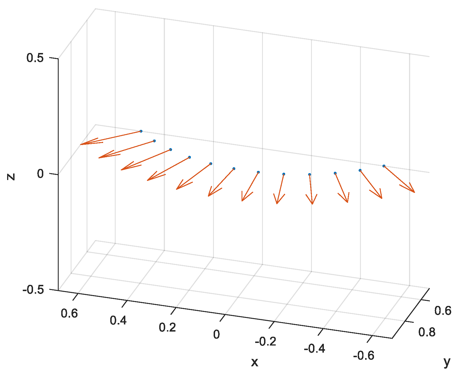
Figure 2 exhibits the configuration of a circular arc array. The conformal array has $N$ elements. Wavelength is denoted by $\lambda$. The element spacing is $\lambda /2$. The direction vector to the $i$th element is expressed by $r_i={[x_i,y_i,z_i]}^T$.

The normalized array factor from $\left(\phi ,\theta \right)$ can be written as

$$s_0\left(\phi ,\theta \right)={[e^{j\frac{2\pi }{\lambda }k\cdot r_1},e^{j\frac{2\pi }{\lambda }k\cdot r_2},\cdots ,e^{j\frac{2\pi }{\lambda }k\cdot r_N}]}^T$$

(3)

In this work, consider the individually-polarized dipole conformal array to be placed tangentially to circumference. $g_i$ represents the element factor of the $i$th element and could be divided into two polarizations which are mutually orthogonal

$$g_i=g_{i\stackrel{\rightharpoonup }{\phi }}\left(\phi ,\theta \right)\overrightarrow{\phi }+g_{i\stackrel{\rightharpoonup }{\theta }}\left(\phi ,\theta \right)\overrightarrow{\theta }$$

(4)

where $g_{i\stackrel{\rightharpoonup }{\phi }}\left(\phi ,\theta \right)$ and $g_{i\stackrel{\rightharpoonup }{\theta }}\left(\phi ,\theta \right)$ stand for the $\overrightarrow{\phi }$ polarized component and $\overrightarrow{\theta }$ polarized component, respectively.

Element factor is expressed in the local coordinate, and ${\tilde{g}}_i\left(\tilde{x},\tilde{y},\tilde{z}\right)$ is known. The accurate formula of the conformal array space steering vector in global coordinates should be obtained. For this purpose, the Euler rotation matrix [30,31] would be used as the transformed tool between the local coordinate system and the global coordinate system for the element factor.

The transformation matrix $\left(x,y,z\right)\Rightarrow \left(\tilde{x},\tilde{y},\tilde{z}\right)$ could be expressed as $T=T_x{T}_y{T}_z$, where

$$T_x=\left[\begin{array}{ccc}1& 0& 0\\ 0& \cos {\sigma }_x& -\sin {\sigma }_x\\ 0& \sin {\sigma }_x& \cos {\sigma }_x\end{array}\right]$$

(5)

$$T_y=\left[\begin{array}{ccc}\cos {\sigma }_y& 0& \sin {\sigma }_y\\ 0& 1& 0\\ -\sin {\sigma }_y& 0& \cos {\sigma }_y\end{array}\right]$$

(6)

$$T_z=\left[\begin{array}{ccc}\cos {\sigma }_z& -\sin {\sigma }_z& 0\\ \sin {\sigma }_z& \cos {\sigma }_z& 0\\ 0& 0& 1\end{array}\right]$$

(7)

Utilizing the transformation matrix, the following could be obtained

$${\tilde{g}}_i\left(\tilde{x},\tilde{y},\tilde{z}\right)=T\cdot g_i\left(x,y,z\right)$$

(8)

Then, the coordinate transformation could be written as

$$g_i\left(x,y,z\right)=T^{-1}\cdot {\tilde{g}}_i\left(\tilde{x},\tilde{y},\tilde{z}\right)$$

(9)

The expression of $g_i$ in the spherical coordinate system $g_{i\stackrel{\rightharpoonup }{\phi }}\left(\phi ,\theta \right)$ and $g_{i\stackrel{\rightharpoonup }{\theta }}\left(\phi ,\theta \right)$ could be obtained using the Cartesian coordinate system by means of the following transformation formula

$$\left[\begin{array}{c}\stackrel{\rightharpoonup }{\phi }\\ \stackrel{\rightharpoonup }{\theta }\end{array}\right]=\left[\begin{array}{ccc}\begin{array}{c}-\sin \phi \\ \sin \theta \cos \phi \end{array}& \begin{array}{c}\cos \phi \\ \sin \theta \sin \phi \end{array}& \begin{array}{c}0\\ -\cos \theta \end{array}\end{array}\right]\left[\begin{array}{c}\stackrel{\rightharpoonup }{x}\\ \stackrel{\rightharpoonup }{y}\\ \stackrel{\rightharpoonup }{z}\end{array}\right]$$

(10)

Now, the conformal array exact space steering vector could be written as follows

$$S_s\left(\phi ,\theta \right)=[G_{\phi }\left(\phi ,\theta \right)\odot s_0\left(\phi ,\theta \right),G_{\theta }\left(\phi ,\theta \right)\odot s_0\left(\phi ,\theta \right)],S_s\in {ℂ}^{N\times 2}$$

(11)

where

$$G_{\phi }\left(\phi ,\theta \right)={[g_{1\stackrel{\rightharpoonup }{\phi }}\left(\phi ,\theta \right),g_{2\stackrel{\rightharpoonup }{\phi }}\left(\phi ,\theta \right),\cdots ,g_{N\stackrel{\rightharpoonup }{\phi }}\left(\phi ,\theta \right)]}^T$$

(12)

$$G_{\theta }\left(\phi ,\theta \right)={[g_{1\stackrel{\rightharpoonup }{\theta }}\left(\phi ,\theta \right),g_{2\stackrel{\rightharpoonup }{\theta }}\left(\phi ,\theta \right),\cdots ,g_{N\stackrel{\rightharpoonup }{\theta }}\left(\phi ,\theta \right)]}^T$$

(13)

It is assumed that the array emits $M$ pulses. $f_r$ stands for pulse repetition frequency. The temporal steering vector could be represented as

$$s_d\left(\phi ,\theta \right)={[1,e^{j\frac{2\pi }{\lambda f_r}2k\cdot v},\cdots ,e^{j\frac{2\pi }{\lambda f_r}2k\cdot v\left(M-1\right)}]}^T$$

(14)

Then, the space-time steering vector for conformal array could be represented by

$$S_{st}\left(\phi ,\theta \right)=s_d\left(\phi ,\theta \right)\otimes S_s\left(\phi ,\theta \right),S_{st}\in {ℂ}^{NM\times 2}$$

(15)

In this paper, it is supposed that the wave is the completely polarized wave. The Jones vector is used to denote the completely polarized wave, and it can be written as

$$e_p=\left[\begin{array}{c}\cos \mu \\ \sin \mu e^{j\beta }\end{array}\right]$$

(16)

where $\mu \in \left[0,\pi /2\right]$ denotes the polarization angle and $\beta \in \left[-\pi ,\pi \right]$ is the polarization phase difference [32].

Finally, the clutter data $c\in {ℂ}^{NM\times 1}$ from $\left(\phi ,\theta \right)$ can be represented as

$$c=\alpha S_{st}\left(\phi ,\theta \right)\cdot e_p=\alpha s\left(\phi ,\theta \right)$$

(17)

where $e_p$ expresses the polarized state of the echo and $\alpha$ denotes the complex amplitude of the clutter scatter.

The received data from the CUT could be denoted as

$$x={\displaystyle \sum _{l=1}^{N_l}{\displaystyle \sum _{c=1}^{N_c}{\alpha }_{l,c}{s}_{l,c}}}+n$$

(18)

where $N_l$ stands for the number of ambiguous range cells and $s_{l,c}=S_{st}\left({\phi }_c,{\theta }_l\right)\cdot e_{p,\left(l,c\right)}$. A clutter range gate could be considered as a superposition of $N_c$ clutter scatters. $n\in {ℂ}^{NM\times 1}$ represents the Gaussian noise vector.

It is supposed that clutter scatters are mutually independent. The ideal CNCM $R\in {ℂ}^{NM\times NM}$ could be written as

$$R={\displaystyle \sum _{l=1}^{N_l}{\displaystyle \sum _{c=1}^{N_c}{\sigma }_{{}_{l,c}}^2{s}_{l,c}}}\cdot s_{l,c}{}^H+{\sigma }_n^2{I}_{NM}$$

(19)

where ${\sigma }_{l,c}^2$ and ${\sigma }_n^2$ represent the power of the $l,c$th clutter scatter and the noise power, respectively.

The STAP weight vector could be acquired through the linearly constrained minimum variance criterion:

$$w=\frac{R_{}^{-1}{s}_t}{s_t^H{R}_{}^{-1}{s}_t}$$

(20)

where the target space-time steering vector could be denoted by $s_t=S_{st}\left({\phi }_0,{\theta }_0\right)\cdot e_{p,t}$.

Due to the unknown interference environment, the CNCM should be estimated from IID training samples, i.e., $\widehat{R}=\frac{1}{L}{\displaystyle \sum _l^L{x}_l{x}_l^H}$, where $L$ stands for the number of the IID training samples. It is often difficult to acquire enough IID training samples, leading to bad STAP performance.

2.2. SR-STAP Formulation

In conventional SR-STAP methods, the angle-Doppler plane is often uniformly divided into $K=N_s{N}_f$ grid points, and $N_f={\rho }_{f}M\left({\rho }_f>1\right)$, $N_s={\rho }_{s}N\left({\rho }_s>1\right)$ denotes the number of normalized Doppler frequencies grids and normalized spatial frequencies grids, respectively. The space-time steering vector from these grid points form the dictionary matrix. However, in the case of conformal array, the formula of the spatial steering vector is different from the planar array. It cannot be expressed in terms of spatial frequency. Thus, the form of the dictionary matrix for conformal array is also different.

The spatial steering vectors of the conformal array are decided by azimuth angle $\phi$, essentially due to the fixed elevation angle $\theta$ within a certain range cell. Therefore, we could divide the azimuth angle to produce spatial grids. In this paper, the angle and Doppler frequencies are also divided into $K=N_s{N}_d$ grids. Let ${\phi }_i=2\pi i/N_s\left(1\le i\le N_s\right)$ and $f_{d,j}=j/N_d\left(-N_d/2\le j\le N_d/2\right)$ represent the uniformly divided azimuth angle and Doppler frequency, respectively. The corresponding time steering vector is

$$s_d\left(f_{d,j}\right)={[1,e^{j2\pi f_{d,j}},\cdots ,e^{j\left(M-1\right)2\pi f_{d,j}}]}^T$$

(21)

The SR-STAP formulation for the SMV condition could be

$$x=Dy+n$$

(22)

where $D$ has following formula:

$$\begin{array}{ll}\hfill D=& \left[s_d\left(f_{d,1}\right)\otimes S_s\left({\phi }_1,{\theta }_k\right),\cdots ,s_d\left(f_{d,1}\right)\otimes S_s\left({\phi }_{N_s},{\theta }_k\right)\right.,\hfill \\ \hfill & \left.\cdots ,s_d\left(f_{d,N_d}\right)\otimes S_s\left({\phi }_{N_s},{\theta }_k\right)\right]\hspace{1em}{ℂ}^{NM\times 2N_s{N}_d}\hfill \end{array}$$

(23)

$y\in {ℂ}^{2N_s{N}_d\times 1}$ can be written as

$$y={\left[{\alpha }_1\cos {\mu }_1,{\alpha }_1\sin {\mu }_1{e}^{j{\beta }_1},\cdots ,{\alpha }_{N_s{N}_d}\cos {\mu }_{N_s{N}_d},{\alpha }_{N_s{N}_d}\sin {\mu }_{N_s{N}_d}{e}^{j{\beta }_{N_s{N}_d}}\right]}^T$$

(24)

Here, $D$ is a dictionary matrix including space-time steering vectors from all grid points. $y$ denotes sparse coefficient vector

In following subsection, we remark that $K=2N_s{N}_d$.

In sparse recovery methods, the SR-STAP problem could be solved by the following

$$\widehat{y}=\underset{y}{\arg \min }{‖y‖}_0, \mathrm{s}.\mathrm{t}. ‖x-Dy‖\le {\epsilon }_1$$

(25)

where ${\epsilon }_1$ represents the fitting error tolerance. We cannot solve (25) directly due to the NP-hard problem. Hence, $l_1$ norm were used in SR-STAP problem.

$$\widehat{y}=\underset{y}{\arg \min }{‖y‖}_1, \mathrm{s}.\mathrm{t}. ‖x-Dy‖\le {\epsilon }_2$$

(26)

where ${\epsilon }_2$ is a user parameter.

3. The Proposed Method

3.1. Derivation of the Proposed Method

In this framework, we adopt the Bayesian perspective to address the linear problem [26]. This will determine the likelihood function of the complex data $x$ and the posterior distribution function of the complex amplitude $y$.

If it is supposed that $n$ in (22) denotes a complex Gaussian vector, the likelihood function of the received data $x$ could be represented as

$$p\left(x|y,\eta \right)=\frac{1}{{\left(\pi \eta \right)}^{NM}}{e}^{-\frac{1}{\eta }{‖x-Dy‖}^2}$$

(27)

Assuming that $y$ is considered to subject to a zeros-mean complex Gaussian prior distribution,

$$y\sim \mathcal{C}\mathcal{N}\left(0,\Gamma \right)$$

(28)

where $\Gamma =\mathrm{Diag}\left(\gamma \right)$. $\gamma ={\left({\gamma }_1,{\gamma }_2,\cdots ,{\gamma }_K\right)}^T$ is a variance vector.

The following is the formula for $y$:

$$p\left(y\left|\Gamma \right.\right)={\pi }^{-K}{\left|\Gamma \right|}^{-1}{e}^{-y^H{\Gamma }^{-1}y}$$

(29)

Given the likelihood for the radar array received data $x$ (27) and the prior (29), the posterior probability density function (PDF) of the complex amplitude $y$ could be expressed as following based on the Bayesian rule:

$$p\left(y\left|x,\Gamma ,\eta \right.\right)=\frac{p\left(x\left|y,\eta \right.\right)p\left(y\left|\Gamma \right.\right)}{{\displaystyle \int p\left(x\left|y,\eta \right.\right)p\left(y\left|\Gamma \right.\right)dy}}$$

(30)

Assuming that the ${\gamma }^{\left(t\right)}$ and ${\eta }^{\left(t\right)}$ are known in the $t$th iteration step, the PDF of $y$ in the $\left(t+1\right)$th iteration could be further represented as:

$$\begin{array}{cc}\hfill p\left(y^{\left(t+1\right)}\left|x,{\Gamma }^{\left(t\right)},{\eta }^{\left(t\right)}\right.\right)& =\frac{p\left(x,y^{\left(t+1\right)}\left|{\Gamma }^{\left(t\right)},\right.{\eta }^{\left(t\right)}\right)}{p\left(x,\left|{\Gamma }^{\left(t\right)},\right.{\eta }^{\left(t\right)}\right)}\hfill \\ \hfill & ={\pi }^{-K}{\left|{\Sigma }^{\left(t+1\right)}\right|}^{-1}{e}^{-{\left(y^{\left(t+1\right)}-{\mu }^{\left(t+1\right)}\right)}^H{\left|{\Sigma }^{\left(t+1\right)}\right|}^{-1}\left(y^{\left(t+1\right)}-{\mu }^{\left(t+1\right)}\right)}\hfill \end{array}$$

(31)

where

$${\mu }^{\left(t+1\right)}={\Gamma }^{\left(t\right)}{D}^H{\Lambda }^{-1}x$$

(32)

$${\Sigma }^{\left(t+1\right)}={\Gamma }^{\left(t\right)}-{\Gamma }^{\left(t\right)}{D}^H{\Lambda }^{-1}D{\Gamma }^{\left(t\right)}$$

(33)

where

$$\Lambda =D{\Gamma }^{\left(t\right)}{D}^H+{\eta }^{\left(t\right)}I$$

(34)

The ${\gamma }^{\left(t\right)}$ could be estimated by a type-II maximum likelihood, which stands for maximizing the marginal likelihood function or other form of it with regard to $\gamma$. The function is the product of (27) and (29) integrated over the complex amplitudes of $y$

$$\begin{array}{cc}\hfill p\left(x\left|\Gamma ,\eta \right.\right)& ={\displaystyle \int p\left(x\left|y,\eta \right.\right)p\left(y\left|\Gamma \right.\right)dy}\hfill \\ \hfill & ={\pi }^{-NM}{\left|C\right|}^{-1}{e}^{-x^H{C}^{-1}x}\hfill \end{array}$$

(35)

The marginal log-likelihood function is

$$\begin{array}{cc}\hfill \mathcal{R}\left(\gamma \right)& =\ln p\left(x\left|\Gamma ,\eta \right.\right)\hfill \\ \hfill & =-\ln \left|C\right|-x^H{C}^{-1}x+\mathrm{constant}\hfill \end{array}$$

(36)

where

$$C=D\Gamma D^H+\eta I$$

(37)

The hyper-parameters $\gamma$ will be obtained by maximizing the log function.

$$\begin{array}{cc}\hfill \widehat{\gamma }& =\underset{\gamma }{\arg \max }\mathcal{R}\left(\gamma \right)\hfill \\ \hfill & =\underset{\gamma }{\arg \min }\mathcal{L}\left(\gamma \right)\triangleq \ln \left|C\right|+x^H{C}^{-1}x\hfill \end{array}$$

(38)

Next, considering that the log-determinant in (38) is concave, a continuous surrogate function will be constructed as the cost function of the optimization problem and the closed solution will be obtained.

The log-determinant term $\ln \left|C\right|$ of $\mathcal{L}\left(\gamma \right)$

$$\ln \left|C\right|=\ln \left|D\Gamma D^H+\eta I\right|=\ln \left|Ddiag\left(\gamma \right)D^H+\eta I\right|$$

(39)

By defining new variables ${\tau }_i=\ln \left({\gamma }_i\right)$ for $i=1,2,\cdots ,K$, the non-convex term $\ln \left|Ddiag\left(\gamma \right)D^H+\eta I\right|$ can be written as

$$\begin{array}{cc}\hfill \ln \left|Ddiag\left(\gamma \right)D^H+\eta I\right|& =\ln \left|{\displaystyle \sum _{i=1}^K{\gamma }_i{d}_i{d}_i{}^H}+\eta I\right|\hfill \\ \hfill & =\ln \left|{\displaystyle \sum _{i=1}^K{e}^{{\tau }_i}{d}_i{d}_i{}^H}+\eta I\right|\hfill \end{array}$$

(40)

where $d_i$ stands for the $i$th column of $D$.

So, utilizing the concept of the conjugate function, the conjugate function of $\ln \left|C\right|$ can be obtained by

$$h^{*}\left(z\right)=\underset{\tau }{\sup }{z}^H\tau -\ln \left|C\right|$$

(41)

Then, based on Fenchel inequality, the following can be obtained

$$\ln \left|C\right|+h^{*}\left(z\right)\ge z^H\tau$$

(42)

With the above, the (38) can be expressed as

$$\widehat{\gamma }=\underset{\gamma }{\min } \underset{\mathbf{z}>0}{\max }{\mathbf{z}}^H\tau -h^{*}(\mathbf{z})+{\mathbf{x}}^H{\mathbf{C}}^{-1}\mathbf{x}$$

(43)

From [26], it can be known that the $\mu$ and $\Sigma$ can also be expressed as

$$\Sigma ={\left({\eta }^{-1}{D}^{H}D+{\Gamma }^{-1}\right)}^{-1}$$

(44)

$$\mu ={\eta }^{-1}\Sigma D^{H}x$$

(45)

Based on matrix inversion lemma and (44) and (45), the following formula can be obtained

$$\begin{array}{cc}\hfill C^{-1}& ={\left(\eta I+D\Gamma D^H\right)}^{-1}\hfill \\ \hfill & ={\eta }^{-1}I-{\eta }^{-1}ID{\left({\Gamma }^{-1}+{\eta }^{-1}{D}^{H}D\right)}^{-1}{D}^H{\eta }^{-1}I\hfill \\ \hfill & ={\eta }^{-1}I-{\eta }^{-1}D\Sigma D^H{\eta }^{-1}\hfill \end{array}$$

(46)

The second term of (38) can be further derived

$$\begin{array}{cc}\hfill x^H{C}^{-1}x& ={\eta }^{-1}{x}^{H}x-{\eta }^{-1}{x}^{H}D\Sigma D^H{\eta }^{-1}x\hfill \\ \hfill & ={\eta }^{-1}{x}^H\left(x-D\mu \right)\hfill \\ \hfill & \begin{array}{l}={\eta }^{-1}{‖x-D\mu ‖}_2^2+{\eta }^{-1}{\mu }^H{D}^H\left(x-D\mu \right)\\ ={\eta }^{-1}{‖x-D\mu ‖}_2^2+{\mu }^H{\Gamma }^{-1}\mu \end{array}\hfill \end{array}$$

(47)

With (43), and discarding irrelevant items, the following expression can be obtained

$$\widehat{\gamma }=\underset{\gamma }{\min } \underset{\mathbf{z}>0}{\max }{\mathbf{z}}^H\tau -h^{*}(\mathbf{z})+{\displaystyle \sum _{i=1}^K\frac{{\left|{\mu }_i\right|}^2}{{\gamma }_i}}$$

(48)

It leads to a so-called iterative min–max process. The lower-bounding is repeatedly minimized, which then tightens the bound. For any fixed ${\tau }^{*}$, given the property of the conjugate function, the ‘=’ of the (42) will be true when $z$ satisfies the following formula.

$$z_i^{\left(t+1\right)}={\left.\frac{\partial \ln \left|C\right|}{\partial {\tau }_i}\right|}_{{\tau }_i^{*}}$$

(49)

The following expression can be obtained

$$\begin{array}{cc}\hfill \frac{\partial \ln \left|C\right|}{\partial {\gamma }_i}& =\frac{\partial \ln \left|C\right|}{\partial \ln \left({\gamma }_i\right)}\frac{\partial \ln \left({\gamma }_i\right)}{\partial {\gamma }_i}\hfill \\ \hfill & \begin{array}{l}=d_i^H{\left(C\right)}^{-1}{d}_i\\ =d_i^H{\left(Ddiag\left(\gamma \right)D^H+\eta I\right)}^{-1}{d}_i\end{array}\hfill \end{array}$$

(50)

Let ${\gamma }_i^{(t)}$ denote the value of ${\gamma }_i$ in the $t$th iteration. With (49) and (50), we can obtain the $z$ in the $t+1$th iteration

$$z_i^{\left(t+1\right)}={\left.\frac{\partial \ln \left|C\right|}{\partial {\tau }_i}\right|}_{{\tau }_i^{\left(t\right)}}={\left.\frac{\partial \ln \left|C\right|}{\partial \ln \left({\gamma }_i\right)}\right|}_{{\gamma }_i^{\left(t\right)}}={\gamma }_i^{\left(t\right)}{d}_i^H{\left(Ddiag\left({\gamma }^{\left(t\right)}\right)D^H+{\eta }^{\left(t\right)}I\right)}^{-1}{d}_i$$

(51)

Then, for the fixed $z^{\left(t+1\right)}$, the (48) can be written as

$$\begin{array}{cc}\hfill \widehat{\gamma }& =\underset{\gamma }{\min } {\left({\mathbf{z}}^{(t+1)}\right)}^H\mathbf{\tau }-h^{*}\left({\mathbf{z}}^{(t+1)}\right)+{\displaystyle \sum _{i=1}^K}\frac{{\left|{\mu }_i\right|}^2}{{\gamma }_i}\hfill \\ \hfill & =\underset{\gamma }{\min } {\left({\mathbf{z}}^{(t+1)}\right)}^H\ln \left(\gamma \right)-h^{*}\left({\mathbf{z}}^{(t+1)}\right)+{\displaystyle \sum _{i=1}^K}\frac{{\left|{\mu }_i\right|}^2}{{\gamma }_i}\hfill \end{array}$$

(52)

The derivative of (52) with respect to ${\gamma }_i$ can be obtained by

$$\frac{\partial \left({\left(z^{\left(t+1\right)}\right)}^H\ln \left(\gamma \right)-h^{*}\left(z^{\left(t+1\right)}\right)+{\displaystyle \sum _{i=1}^K\frac{{\left|{\mu }_i\right|}^2}{{\gamma }_i}}\right)}{\partial {\gamma }_i}=\frac{z_i^{\left(t+1\right)}}{{\gamma }_i}-\frac{{\left|{\mu }_i\right|}^2}{{\gamma }_i^2}$$

(53)

Set (53) to zero, and the following update rule can be acquired

$${\gamma }_i^{\left(t+1\right)}={\left(z_i^{\left(t+1\right)}\right)}^{-1}{\left|{\mu }_i^{\left(t+1\right)}\right|}^2$$

(54)

3.2. The Estimation of $\eta$

In the above, the value of $\eta$ is assumed to be known; here, we need to estimate $\eta$. This procedure has been researched in previous work [28]. For convenience, the final result will be presented directly. In each iteration, $\eta$ is updated by

$${\eta }^{(t+1)}=\frac{{‖x-D{\mu }^{(t+1)}‖}_2^2+{\eta }^{(t)}{\displaystyle \sum _{i=1}^K{\gamma }_i^{\left(t\right)}}{d}_i^H{\left(C^{\left(t\right)}\right)}^{-1}{d}_i}{NM}$$

(55)

Since the proposed method is an iterative process, initializing the hyper-parameter ${\gamma }_i^{\left(0\right)}={\left|d_i^{H}x\right|}^2/{\left|d_i^H{d}_i\right|}^2$, for $i=1,2,\cdots ,K$, and $\eta$ could be initialized with a positive scalar. We use ${\eta }^{\left(0\right)}=1$.

The convergence criterion of the iteration is followed

• The number of iterations reaches the upper limit.
• The estimate of hyper-parameter $\gamma$ meet ${‖{\gamma }^{(t)}-{\gamma }^{(t-1)}‖}_2/{‖{\gamma }^{(t)}‖}_2<\delta$, where $\delta$ is a small positive number.

By the proposed method, the relatively precise estimate of $\mathsf{\mu }$ and $\eta$ can be obtained. The estimated CNCM expresses as follows:

$$R={\displaystyle \sum _{i=1}^K\left({\left|{\mu }_i\right|}^2\right)d_i{d}_i^{\mathrm{H}}}+\eta I$$

(56)

The pseudo-code for the NFSBL method is given in Algorithm 1.

Algorithm 1: NFSBL Method
Step 1	Input data $x$ and dictionary matrix $D$
Step 2	Initialize $\gamma$ and $\eta$
Step 3	Update the mean vector $\mathsf{\mu }$ using (32)
Step 4	Update $\gamma$ and $\eta$ using (54) and (55), respectively
Step 5	Repeat step 3–4 until the convergence criterion is met
Step 6	Calculate CNCM $R={\displaystyle \sum _{i=1}^K\left({\left|{\mu }_i\right|}^2\right)d_i{d}_i^{\mathrm{H}}}+\eta I$
Step 7	Compute STAP weight $w$

3.3. Extension to the MMV Case

With above discussion, it has been known that the (23) is the dictionary matrix which contains the steering vectors of $k$th range cell. By carrying out some calculations, a conclusion can be drawn that the elevation angle from the neighboring range cells are only slightly different from the elevation angle of $k$th range cell. In this work, the proposed method can approximatively consider that the dictionary matrix in (23) also contains the steering vectors of neighboring range cells. Then, the proposed method could be developed to the MMV case.

The SR formulation for MMV case is

$$X=DY+N$$

(57)

where $X=\left[x_1,x_2,\cdots ,x_L\right]$ and $Y,N$ have similar structures.

In the MMV case, the estimate of the $Y$ is denoted by the matrix form of (32).

$${\Psi }^{\left(t+1\right)}={\Gamma }^{\left(t\right)}{D}^H{\Lambda }^{-1}X$$

(58)

where $\Psi =\left[{\mu }_1,{\mu }_2,\cdots ,{\mu }_L\right]$.

Similarly, (54) and (55) could be directly developed to the MMV case and the following can be obtained

$${\gamma }_i^{\left(t+1\right)}={\left(z_i^{\left(t+1\right)}\right)}^{-1}\frac{1}{L}{\displaystyle \sum _{l=1}^L{\left|{\mu }_{l,i}^{\left(t+1\right)}\right|}^2}$$

(59)

$${\eta }^{(t+1)}=\frac{\frac{1}{L}{\displaystyle \sum _{l=1}^L{‖x-D{\mu }_l^{\left(t+1\right)}‖}_2^2}}{NM-{\displaystyle \sum _{i=1}^K{\gamma }_i^{\left(t\right)}}{d}_i^H{\left(C^{\left(t\right)}\right)}^{-1}{d}_i}$$

(60)

The hyper-parameter $\gamma$ could be initialized as ${\gamma }_i^{\left(0\right)}=\frac{1}{L}{\displaystyle \sum _{l=1}^L{\left|d_i^H{x}_l\right|}^2/{\left|d_i^H{d}_i\right|}^2}$.

The estimated CNCM expresses as follows

$$R=\frac{1}{L}{\displaystyle \sum _{l=1}^L{\displaystyle \sum _{i=1}^K\left({\left|{\mu }_{l,i}\right|}^2\right)d_i{d}_i^{\mathrm{H}}}+\eta I}$$

(61)

The proposed method is summarized in Algorithm 2.

Algorithm 2: M-NFSBL Method
Step 1	Input data $X$ and dictionary matrix $D$
Step 2	Initialize $\gamma$ and $\eta$
Step 3	Update the mean matrix $\Psi$ using (58)
Step 4	Update $\gamma$ and $\eta$ using (59) and (60), respectively
Step 5	Repeat steps 3–4 until the convergence criterion is met
Step 6	Calculate CNCM $R=\frac{1}{L}{\displaystyle \sum _{l=1}^L{\displaystyle \sum _{i=1}^K\left({\left|{\mu }_{l,i}\right|}^2\right)d_i{d}_i^{\mathrm{H}}}+\eta I}$
Step 7	Compute STAP weight $w$

4. Discussion

4.1. Complexity Analysis

In this work, the computational complexity will be researched in the MMV condition. In order to obtain better readability, some definitions of important parameters will be re-emphasized here. $K$ is the number of the space-time vector of the dictionary matrix. $L$ stands for the number of IID training samples. $M$ represents the pulse number and $N$ expresses the element number. The number of complex multiplications is used as the evaluation metric of the computational complexity. For convenience, we ignore the low-order multiplications. From the above analysis, the proposed method contains the calculation of $\Psi$, $\gamma$, and $\eta$ in an iteration. Therefore, it is found that the computational complexity of M-NFSBL method can be denoted as $o\left(KL+\left(3K+2KL+L\right)MN+3K{\left(MN\right)}^2+{\left(MN\right)}^3\right)$. The computational complexity of other SR methods are shown in

Table 1. The computational complexity of various methods.

Algorithm	Computational Load for an Iteration
M-CVX	$o\left({\left(KL\right)}^3\right)$
M-SBL	$o\left(K+K^2+KL+\left(2K+2KL+K^2+L\right)MN+2K{\left(MN\right)}^2+{\left(MN\right)}^3\right)$
M-FCSBL	$o\left(\left(4K+2KL+L\right)MN+5K{\left(MN\right)}^2+{\left(MN\right)}^3\right)$
M-NFSBL	$o\left(KL+\left(3K+2KL+L\right)MN+3K{\left(MN\right)}^2+{\left(MN\right)}^3\right)$

.

Computational complexity could be viewed as a function of the number of pulses. Figure 3 express the computational complexity of the various methods. If it is supposed that $K=1600$, $N=8$, and $L=5$, it is concluded that the computational complexity of the M-NFSBL method is more advantageous.

4.2. Convergence Analysis

The above discussion shows that the cost function could be written as $\mathcal{L}\left(\gamma \right)={\left(z\right)}^H\ln \left(\gamma \right)-h^{*}\left(z\right)+x^H{C}^{-1}x$ in the every iteration so long as $z$ satisfied the (51), which is a function with respect to $\gamma$. We could obtain that $\mathcal{L}\left({\gamma }^{\left(t+1\right)}\right)\le \mathcal{L}\left({\gamma }^{\left(t\right)}\right)$ from (53) and (54). According to [33], we know that $\mathcal{L}\left(\gamma \right)$ has a bound. It is therefore a monotonically decreasing function and indicates that the proposed method converges.

The following simulation experiments demonstrate that the proposed method converges faster than SBL.

5. Simulation Results

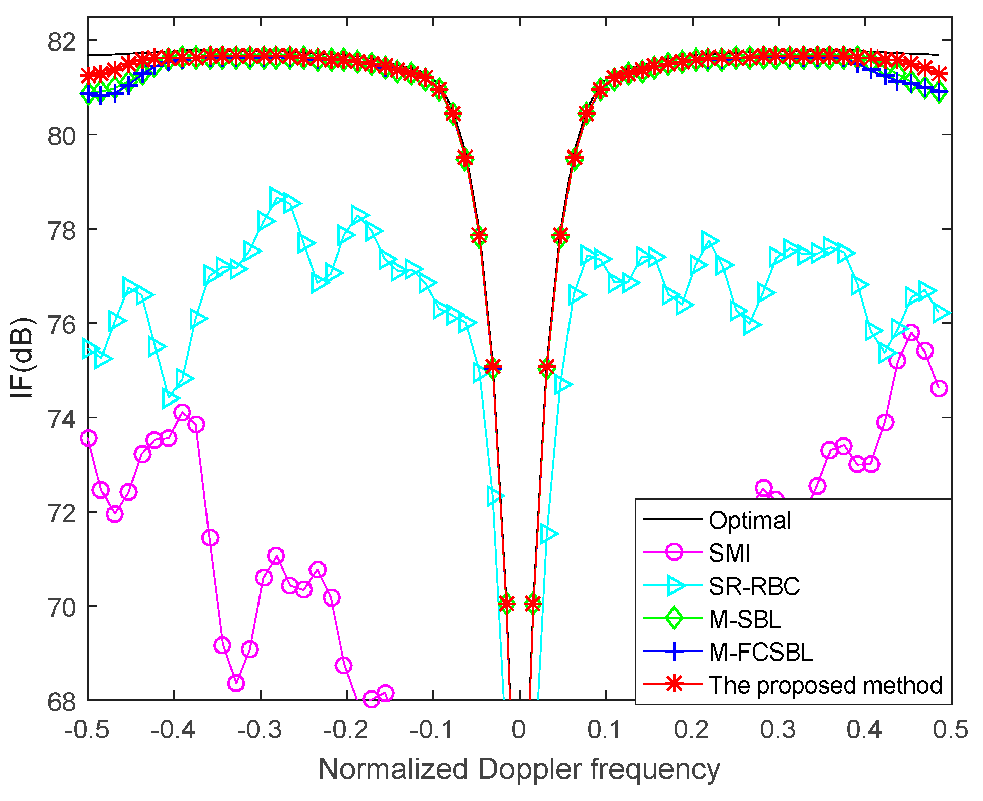
The STAP performance of the proposed method will be assessed in this section. Given a side-looking conformal array radar, such as shown in Figure 2, the direction of the desired signal is ${\phi }_0={90}^{\mathrm{o}}$, ${\theta }_0=0^{\mathrm{o}}$ and the polarization angle and polarization phase difference of the desired signal are $\mu =\pi /2$ and $\beta =0$. The relevant radar system parameters are provided in

Table 2. Radar parameters.

Parameter	Value	Unit
Pulse number	16	-
Element number	12	-
Platform velocity	200	m/s
Wavelength	0.2	m
Bandwidth	5	MHz
CNR	60	dB
Distance between elements	0.1	m
Pulse repetition frequency	5000	Hz
Platform height	3000	m

. The 300th range cell has been selected to be CUT. Then, the IF is used as the evaluation metric of STAP performance:

$$\mathrm{IF}=\frac{{\left|w^{\mathrm{H}}s\right|}^2}{w^{\mathrm{H}}Rw}\frac{\mathrm{tr}\left(R\right)}{s^{\mathrm{H}}s}$$

(62)

where $R$ represents the ideal CNCM.

As mentioned in Section 3.3, the elevation angle corresponding to the neighboring range cells are only slightly different from the elevation angle of the $k$th range cell. So, in the MMV case, a small number of range cells are used as the data for multiple snapshots, and the number is set as $L=5$.

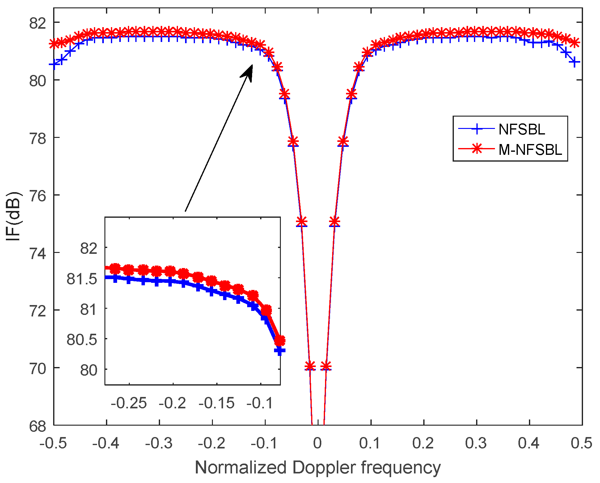
Figure 4 illustrates the IF curves of the proposed method in the SMV condition and the MMV condition. It has been shown that the M-NFSBL method has slight advantage (about 0.2 dB). When the Doppler frequency is close to $\pm 0.5$ Hz, the M-NFSBL method shows obvious superior performance.

So, in the following discussion, the simulation experiments exhibit the performance with different methods in the MMV case. These methods include the sample matrix inversion method (SMI), the registration-based compensation method with sparse recovery (SR-RBC), a multiple sparse Bayesian learning with fast-convergence method (M-FCSBL), and a multiple sparse Bayesian learning method (M-SBL), and the proposed method will be evaluated with the simulated data in the ideal and non-ideal cases.

The cost function $\ln \left|C\right|+\mathrm{Tr}\left(C^{-1}{R}_{ML}\right)$ will be utilized to assess the convergence performance of different methods. $R_{ML}=X{X}^H/L$. Three methods will be considered here: M-SBL, M-FCSBL, and the proposed method.

As shown in Figure 5, it could be found that the M-FCSBL and the proposed method converge faster and need about 20 iterations to obtain a steady state. The M-SBL need more iterations to converge to the steady state.

5.1. Ideal Condition

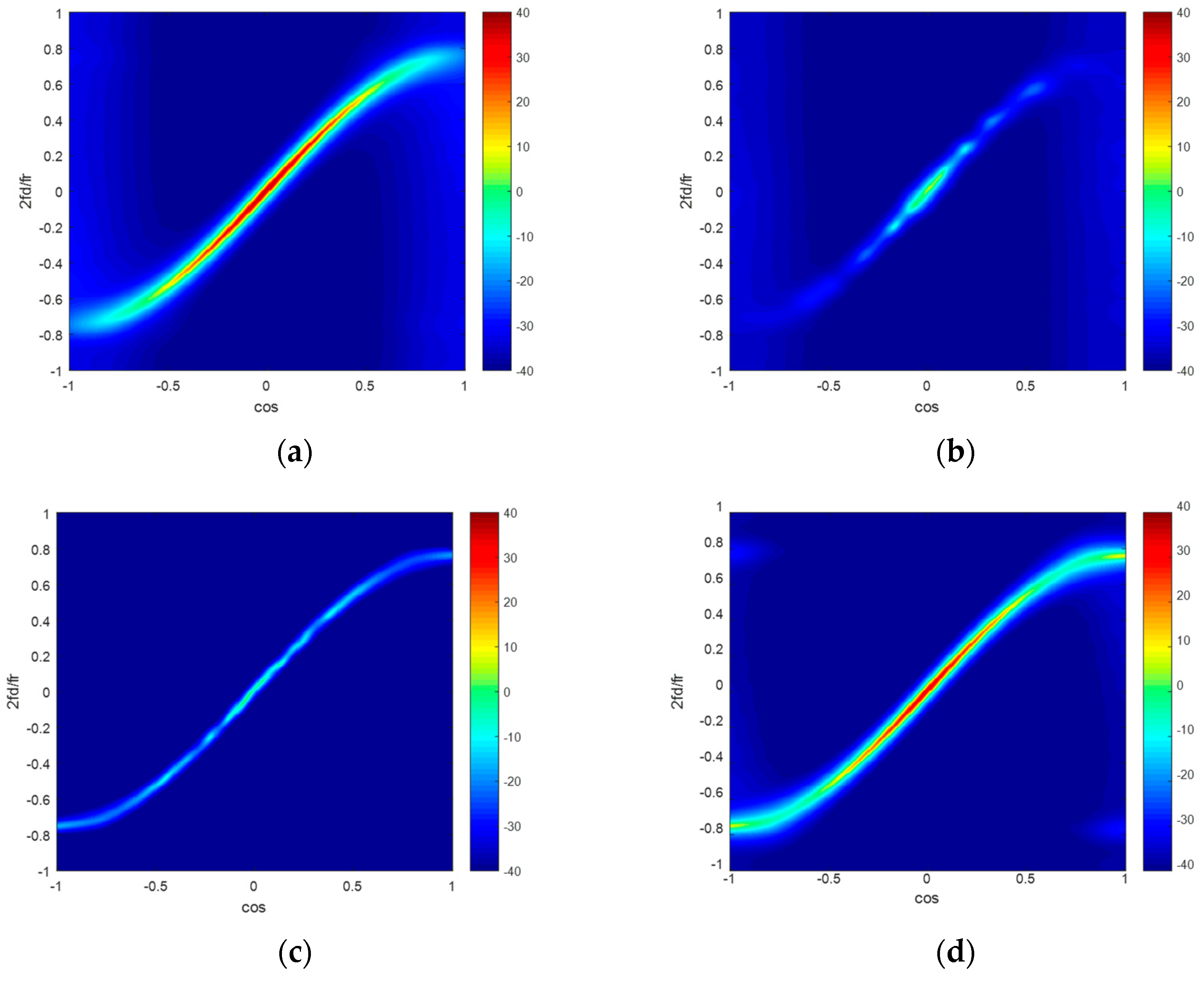
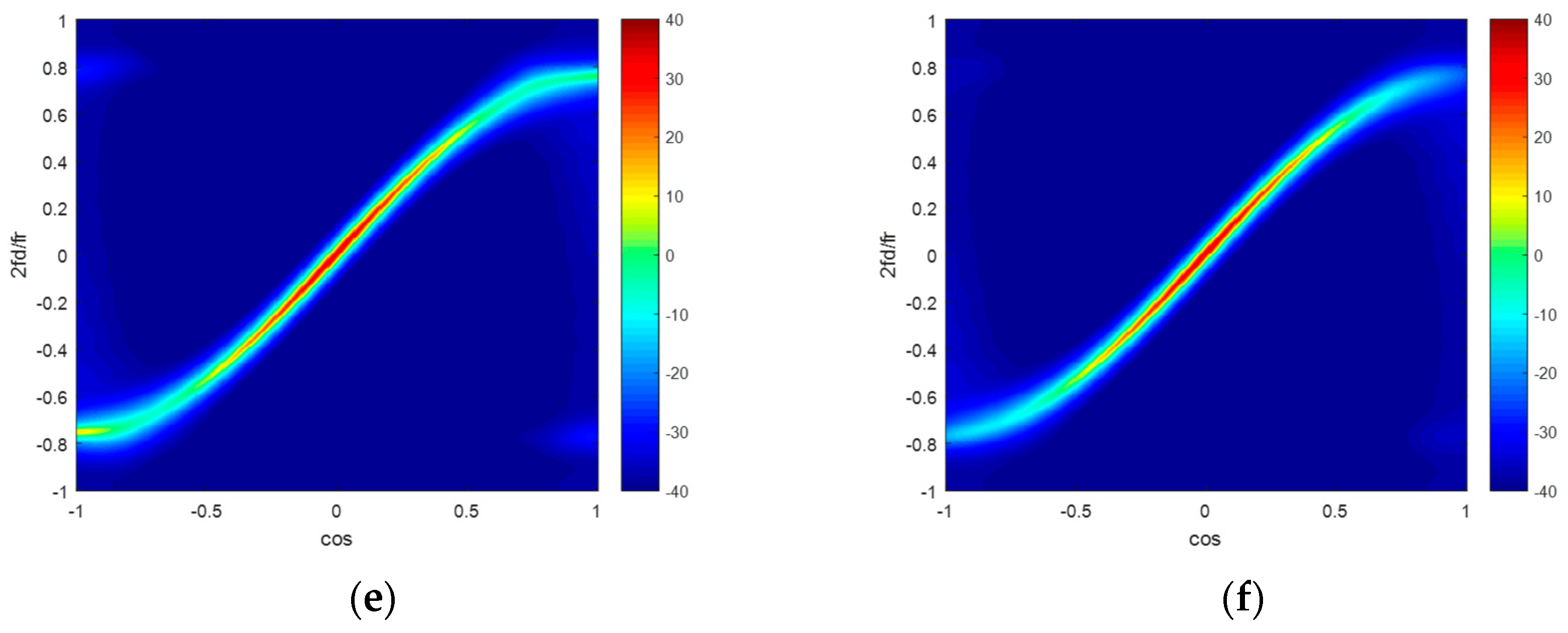
In this subsection, the clutter Capon spectrums of various methods have been given. In order to avoid the matrix singularity caused by inadequate training samples, the diagonal load method has been applied in the SMI and SR-RBC methods. From Figure 6a–f, we can know that the recovered clutter spectrums of the SMI method and the SR-RBC method are disappointing due to the inadequate training samples. It can be known that the more accurate Capon spectrums are acquired by the M-SBL method, the M-FCSBL method, and the proposed method.

Figure 7 depicts the IF comparison by different methods. It can be observed that excellent performance could be acquired by the M-SBL method, the M-FCSBL method, and the proposed method. This further indicates that the proposed method does not change the clutter suppression performance of the original M-SBL method with the faster converge rate and lower computational complexity.

5.2. Non-Ideal Condition

In this subsection, a non-ideal condition with the presence of gain and phase error will be taken into account. This will lead to mismatch between the dictionary matrix and the real space-time steering vector. The estimated CNCM will be inaccurate.

As shown in Figure 8, the non-ideal case is introduced with 0.02 gain error and 0.2° phase error in these methods. From Figure 8a–f, it can also be found that the estimated clutter Capon spectrums from the M-SBL method, the M-FCSBL method, and the proposed method are more similar to the Capon spectrum estimated by exact CNCM.

Figure 9 expresses the IF comparison by different methods with gain and phase error. Compared with the optimal IF curve, the M-SBL method, the M-FCSBL method, and the proposed method have little performance degradation and the main lobe notch has been slightly widened. However, the performance of these methods is still superior to other traditional methods.

6. Conclusions

In this paper, a novel fast sparse Bayesian learning method named NFSBL was presented with the goal of improving the performance of suppressing clutter for conformal arrays. The novel method introduces the concept of the conjugate function to construct a surrogate function for the SBL cost function. This method improves the convergence speed of the SBL method. The proposed NFSBL method in the MMV condition has also been developed; it expresses a lower computational load compared with other SR-STAP methods. All of the simulation experiments have demonstrated that the M-NFSBL method has a superior performance in STAP.

References

1. Hersey, R.K.; Melvin, W.L.; McClellan, J.H.; Culpepper, E. Adaptive ground clutter suppression for conformal array radar systems. IET Radar Sonar Navig. 2009, 3, 357–372. [Google Scholar] [CrossRef]
2. Ward, J. Space-Time Adaptive Processing for Airborne Radar; Technical Report, 1015; MIT Lincoln Laboratory: Lexington, MA, USA, 1994. [Google Scholar]
3. Klemm, R. Principles of Space-Time Adaptive Processing, 3rd ed.; IET: London, UK, 2006. [Google Scholar]
4. Wu, Y.F.; Wang, T.; Wu, J.X. Robust training samples selection algorithm based on spectral similarity for space-time adaptive processing in heterogeneous interference environments. IET Radar Sonar Navig. 2015, 9, 778–782. [Google Scholar]
5. Reed, I.S.; Mallett, J.D.; Brennan, L.E. Rapid convergence rate in adaptive arrays. IEEE Trans. Aerosp. Electron. Syst. 1974, 10, 853–863. [Google Scholar] [CrossRef]
6. Klemm, R. The Applications of Space-Time Adaptive Processing, 2nd ed.; IEE Press: Stevenage, UK, 2004. [Google Scholar]
7. Himed, B.; Zhang, Y.; Hajjari, A. STAP with angle-Doppler compensation for bistatic airborne radars. In Proceedings of the IEEE National Radar Conference, Long Beach, CA, USA, 25 April 2002. [Google Scholar]
8. Melvin, W.; Himed, B.; Davis, M. Doubly adaptive bistatic clutter filtering. In Proceedings of the IEEE National Radar Conference, Hunstville, AL, USA, 8 May 2003. [Google Scholar]
9. Melvin, W.; Davis, M. Adaptive cancellation method for geometry-induced nonstationary bistatic clutter environment. IEEE Trans. Aerosp. Electron. Syst. 2007, 43, 651–672. [Google Scholar] [CrossRef]
10. Han, X.; Luo, T.; Yu, W.; Wu, M. Space-time adaptive processing for airborne radar with conformal array. In Proceedings of the IET International Radar Conference, Hangzhou, China, 14–16 October 2015; pp. 5–10. [Google Scholar]
11. Varadarajan, V.; Krolik, J.L. Joint space-time interpolation for distorted linear and bistatic array geometries. IEEE Trans. Signal Process. 2006, 56, 848–860. [Google Scholar] [CrossRef]
12. Ries, P.; Lapierre, F.D.; Verly, J.G. Geometry-induced range-dependence compensation for bistatic STAP with conformal arrays. IEEE Trans. Aerosp. Electron. Syst. 2011, 47, 275–294. [Google Scholar] [CrossRef]
13. Klemm, R. Adaptive airborne MTI: An auxiliary channel approach. IEEE Proc. F Commun. Radar Signal Process. 1987, 134, 269–276. [Google Scholar] [CrossRef]
14. Wang, Y.X.; Li, X.M.; Gao, W. Dimension-reduced bi-iterative space-time adaptive processing method for airborne radar. J. Eng. 2019, 2019, 8138–8141. [Google Scholar] [CrossRef]
15. Wang, X.; Yang, Z.; Yang, J.X. Reduced-dimension space-time adaptive processing for airborne radar with co-prime array. J. Eng. 2019, 2019, 5971–5974. [Google Scholar] [CrossRef]
16. Hua, Y.; Nikpour, M.; Stoica, P. Optimal reduced rank estimation and filtering. IEEE Trans. Signal Process. 2001, 49, 457–469. [Google Scholar]
17. Sarkar, T.K. A deterministic least-squares approach to space-time adaptive processing (STAP). IEEE Trans. Antennas Propag. 2001, 49, 91–103. [Google Scholar] [CrossRef]
18. Melvin, W.L.; Showman, G.A. An approach to knowledge-aided covariance estimation. IEEE Trans. Aerosp. Electron. Syst. 2006, 42, 1021–1042. [Google Scholar] [CrossRef]
19. Wicks, M.C.; Rangaswamy, M.; Adve, R.; Hale, T.B. Space-time adaptive processing: A knowledge-based perspective for airborne radar. IEEE Signal Process. Mag. 2006, 23, 51–65. [Google Scholar] [CrossRef]
20. Yang, Z.C.; Li, X.; Wang, H.Q.; Jiang, W.D. On clutter sparsity analysis in space-time adaptive processing airborne radar. IEEE Geosci. Remote Sens. Lett. 2013, 10, 1215–1218. [Google Scholar]
21. Sen, S. Low-rank matrix decomposition and spatio-temporal sparse recovery for STAP radar. IEEE J. Sel. Top. Signal Process. 2015, 9, 1510–1523. [Google Scholar] [CrossRef]
22. Tibshirani, R. Regression shrinkage and selection via the lasso. J. R. Stat. Soc. 1996, 58, 267–288. [Google Scholar] [CrossRef]
23. Candés, E. The restricted isometry property and its implications for compressed sensing. Comptes Rendus Math. 2008, 346, 589–592. [Google Scholar] [CrossRef]
24. Sun, K.; Meng, H.D.; Fabian, D.L. Registration-based compensation using sparse representation in conformal-array STAP. Signal Process. 2011, 91, 2268–2276. [Google Scholar] [CrossRef]
25. Tao, F.Y.; Wang, T.; Wu, J.X.; Su, Y.Y. A knowledge aided SPICE space time adaptive processing method for airborne radar with conformal array. Signal Process. 2018, 152, 54–62. [Google Scholar] [CrossRef]
26. Tipping, M.E. Sparse Bayesian learning and the relevance vector machine. J. Mach. Learn. 2001, 1, 211–244. [Google Scholar]
27. Wipf, D.P.; Rao, B.D. An empirical Bayesian strategy for solving the simultaneous sparse approximation problem. IEEE Trans. Signal Process. 2007, 55, 3704–3716. [Google Scholar] [CrossRef]
28. Wang, Z.T.; Xie, W.C.; Duan, K.Q.; Wang, Y.L. Clutter suppression algorithm based on fast converging sparse Bayesian learning for airborne radar. Signal Process. 2017, 130, 159–168. [Google Scholar] [CrossRef]
29. Ren, B.; Wang, T. Space-time adaptive processing based on modified sparse learning via iterative minimization for conformal array radar. Sensors 2022, 22, 6917. [Google Scholar] [CrossRef] [PubMed]
30. Burger, H.A. Use of Euler-Rotation angles for generating antenna patterns. IEEE Antennas Propag. Mag. 1995, 37, 56–63. [Google Scholar] [CrossRef]
31. Milligan, T. More applications of Euler rotation angles. IEEE Antennas Propag. Mag. 1999, 41, 78–83. [Google Scholar] [CrossRef]
32. Zhuang, Z.W. Radar Polarization Information Processing and Application, 1st ed.; National Defense Industrial Press: Beijing, China, 1999. [Google Scholar]
33. Wipf, D.; Nagarajan, S. A new view of automatic relevance determination. In Advances in Neural Information Processing Systems 20; MIT Press: New York, NY, USA, 2008. [Google Scholar]
Figure 1. Abridged general view of airborne radar system.
Remotesensing 15 02824 g001
Figure 2. Geometry configuration.
Remotesensing 15 02824 g002
Figure 3. Computational complexity of different methods.
Remotesensing 15 02824 g003
Figure 4. IF curves with SMV and MMV.
Remotesensing 15 02824 g004
Figure 5. Value of the cost function.
Remotesensing 15 02824 g005
Figure 6. Clutter Capon spectrums of various methods: (a) exact CNCM; (b) SMI; (c) SR-RBC; (d) M-SBL; (e) M-FCSBL; (f) the proposed method.
Remotesensing 15 02824 g006aRemotesensing 15 02824 g006b
Figure 7. The IF comparison of different methods in ideal condition.
Remotesensing 15 02824 g007
Figure 8. Clutter Capon spectrums of various methods with gain and phase error: (a) exact CNCM; (b) SMI; (c) SR-RBC; (d) M-SBL; (e) M-FCSBL; (f) the proposed method.
Remotesensing 15 02824 g008
Figure 9. The IF comparison of different methods in non-ideal condition.
Remotesensing 15 02824 g009