CALIOP-Based Evaluation of Dust Emissions and Long-Range Transport of the Dust from the Aral−Caspian Arid Region by 3D-Source Potential Impact (3D-SPI) Method

Abstract

The average monthly profiles of the dust extinction coefficient (ε) were analyzed according to the CALIOP lidar data from 2006–2021 for 24 cells (size of 2° × 5°) in the Aral-Caspian arid region (ACAR; 38–48°N, 50–70°E). Using the NOAA HYSPLIT_4 trajectory model and the NCEP GDAS1 gridded (resolution of 1° × 1°) archive of meteorological data, the array of >1 million 10-day forward trajectories (FTs) of air particles that started from the centers of the ACAR cells was calculated. On the basis of the FT array, the average seasonal heights of the mixed layer (ML) for the ACAR cells were reconstructed. Estimates of the average seasonal dust optical depth (DOD) were obtained for ACAR’s lower troposphere, for ACAR’s ML (“dust emission layer” (EL)), and for the lower troposphere above the ML (“dust transit layer” (TL)) above each of the ACAR cells. Using the example of ACAR, it is shown that the analysis of DOD for the EL, TL and the surface layer (SL; the first 200 m AGL) makes it possible to identify dusty surfaces that are not detected on DOD diagrams for the entire atmospheric column, as well as regions where the regular transport of aged dust from remote sources can generate false sources. Based on FT array, the fields of the potential contribution of both the ACAR’s dust transit and the ACAR’s dust emission layers as well as of the entire ACAR’s lower troposphere into the DOD of the surrounding and remote regions are retrieved using the original method of potential impact of a three-dimensional source (3D-PSI). It has been found out that ACAR dust spreads over almost the entire Northern Hemisphere; the south and southeast regions of the ACAR are subject to the maximum impact of the ACAR dust. Quantitative estimates of the potential contribution of ACAR dust to the regional DODs are given for a number of control sites in the Northern Hemisphere. The results could be useful for climatological studies.

1. Introduction

Atmospheric aerosols, including dust, affect air quality, human and animal health [1,2,3,4], vegetation productivity [5,6], solar and thermal radiation balance and climate [7,8,9,10,11,12], ice composition and glaciers [13,14,15], and snow cover [16,17,18,19]. Dust is the largest contributor to global atmospheric aerosol mass [8,20,21,22,23], and in the 20th century, according to the estimates of [3], the global dust content in the atmosphere more than doubled. The main dust source is the surface of arid regions of the desert belt of North Africa, the Middle East, and Central Asia [24,25,26]. The main mechanism of desert dust emission is wind removal of mineral particles from the underlying surface [27,28]. Under weak wind conditions, convective processes (including vortexes) become significant drivers of dust emissions, which was found numerically [29,30,31,32] and confirmed experimentally [33,34,35,36,37].

Dust impacts greatly on the environment in the same regions where it is emitted from the underlying surface and in surrounding areas (see, for example, [38]). At the same time, because of the relatively small particle size of transported dust particles (median aerodynamic diameter in the range of 3–7 µm according to [39]), they are carried out by turbulent and convective flows from the near-surface layer to the atmospheric boundary layer (ABL). Subsequently, dust is transported by winds over intercontinental distances, affecting the troposphere and the objects at the underlying surface of a significant part, if not all, of the Northern Hemisphere [26,40,41]. According to [42], Saharan dust is found over the tropical waters of the Atlantic Ocean at a distance of 3500–4000 km from the African coast. Dust reaches the western (through the Pacific Ocean; ~19,000 km en route [43]) and eastern (through the Atlantic Ocean) coasts of North America, in the Yucatan Peninsula [44]. It is found near the Caribbean Islands and the Amazon Basin [39,45,46,47,48] and over Europe [49]. Dust from the deserts of Central Asia reaches North America (through the Pacific Ocean [50] and through the Arctic [51]), Russian and North American Arctic regions [51,52], European [53,54] and Asian [52,53] territories of Russia and affects large areas of Southeast Asia [52,55]. According to [56], backward trajectories for cases of extreme contents of chemical elements characteristic of mineral dust (Al, Fe, Mn, Ti, Cr, and V) indicate that the Svalbard glaciers are exposed to the dust from Eurasia, including from Kazakhstan. According to [57], dust transported from Central Asia (Taklimakan Desert) is indicated as one of the likely reasons for pollution of the Greenland glaciers.

The long-range dust transport from the desert belt to the territory of Russia has not been studied enough; less than 1000 km from the southern borders of Russia is the Aral−Caspian Arid Region (ACAR), which includes vast dust sources, from the deserts of Karakum, Kyzylkum, and Aralkum, the desert on the site of Aral Sea’s dried bottom [58,59]. The purpose of this work is to assess the dust transported from ACAR to the surrounding and remote territories in the last two decades. ACAR’s “sphere of influence” in terms of [60] is reconstructed based on both the modeling of Lagrangian trajectories of air particles and the vertical profiles of the tropospheric dust extinction coefficient by CALIOP lidar sounding data from the NASA/CNES CALIPSO satellite that are conjoined in the original three-dimensional source potential impact (3D-SPI) method.

2. Materials and Methods

2.1. The Region under Study

The studied region and source of the dust, namely ACAR, occupies ~1.8 million km² in the west of Central Asia in an area approximated by rectangle of 37–49°N, 50–70°E (1332 × 1623 km²; see Figure 1).

This is a predominantly flat territory; highlands are only near the ACAR’s southern (cell 2; north of Iranian Highlands) and southeastern (cells 4 and 8; Fann Mountains and Pamir Alai) borders. As can be seen from Figure 1, the ACAR territory is located mainly (~95%) in Kazakhstan, Uzbekistan, and Turkmenistan; the rest covers the west of Tajikistan and northern parts of Iran and Afghanistan. The sandy deserts of Karakum and Kyzylkum; the sandy-salt Aralkum Desert; the stony-clayey Ustyurt Plateau, Solonchaks, and Takyrs; and semi-arid steppes cover about ~80% of ACAR territory. The first three deserts are considered in [38] as the main dust sources of the region, among which, according to [62], Aralkum Desert dominates. The Karakum and Kyzylkum Deserts are “aged” deserts, and it can be expected that most of the dust capable of long-range transport has already left the deserts’ surfaces, while a significant part of the south and east of the Aralkum Desert is formed by vast alluvial deposits in the former estuaries of the Amu Darya and Syr Darya Rivers, which have been experienced erosion relatively recently. According to [63], the density of point dust emission sources (dust hotspots) in the south and east of the Aralkum Desert is one of the highest in the ACAR and in Central Asia. Based on the average annual runoff and water turbidity [64], the average solid runoff of the Amu Darya and Syr Darya Rivers in the first half of the 20th century has been estimated as ~100 × 10⁶ and ~12 × 10⁶ tons per year, respectively (see, e.g., [65]), of clayey matter washed off in the upper parts of these rivers. If the past solid runoff was comparable with the estimates, it can be expected that over the last centuries, the bottom of the Aral Sea near the rivers’ estuaries has accumulated tens, if not hundreds, of billions of tons of particulate matter. In addition, Aral Sea salt deposits, according to [66], can reach up to 6 × 10⁹ tons. With an average annual dust removal of 150 × 10⁶ tons per year [67,68], these alluvial deposits can emit dust at the same intensity now for decades.

The stony-argillaceous Ustyurt Plateau in [63] is considered to be predominantly a dust sink, while [60] the dust emission in spring and summer is significant here as it is in the Karakum Desert. The steppes of northern and western Kazakhstan may also be a dust source, especially in dry years.

Regular study of dust emissions in ACAR deserts is difficult because of their difficult accessibility and extreme conditions throughout the year. In the recent decades, episodic and sporadic field studies have been carried out on the distribution function, chemical composition, and optical parameters of aerosol in the surface layer and in the atmospheric column in Tajikistan [69,70,71,72,73], as well as the optical and microphysical characteristics of dust in the Aralkum Desert [74]; dust deposition at various sites of the ACAR [38,75]; horizontal flows dust, sand, and salt from Aralkum Desert [62]; lidar-derived parameters of aerosol (including dust) in the atmosphere in Tajikistan [76,77]; fine aerosol emission under convective conditions in Aralkum Desert [78]; and vertical mass fluxes and size distributions of dust particles during wind and convective/vortex dust emissions from Aralkum Desert [35,79]. The only station of AERONET (AErosol RObotic NETwork [80]) is located in Dushanbe (Tajikistan; see [81]) on the southeastern periphery of ACAR. Therefore, only satellites can provide regular experimental data on aerosol parameters in the troposphere of the entire ACAR.

The most detailed time (daily data) and space (resolution of up to 1 × 1 km²) modern data on the aerosol optical depth (AOD) of the total aerosol comes from the MODIS (MODerate resolution Infrared Spectroradiometer) instrument mounted at the Terra (since 2000) and Aqua (since 2002) satellites [82]. Because of the lack of information on the vertical aerosol profile and the proportion of dust in AOD, MODIS-based dust outputs from the surface may be overestimated [63]. Moreover, according to [63], there is not correct AOD retrieval for an ephemeral water body such as the Aral Sea. The second longest operating data source is the CALIOP lidar installed on the NASA/CNES CALIPSO satellite [83], which, since June 2006, has been providing instantaneous vertical profiles of the extinction coefficient of total aerosols and its components including dust, but with a lower resolution in time and space than that of MODIS.

2.2. Satellite Data

CALIOP (Cloud-Aerosol LIdar with Orthogonal Polarization; see [83]) measures the vertical profiles of the aerosol extinction coefficient, ε [km⁻¹], at a frequency of ~20 Hz at wavelengths of 532 and 1064 nm. ε profiles are retrieved for the total tropospheric (and stratospheric) aerosols, as well as for tropospheric aerosol fractions (dust, smoke, polluted dust, etc.). The CALIPSO satellite flies in a sun-synchronous orbit (inclination of 98.05°) at an altitude of ~700 km, crossing the Equator around 13:30 p.m. and 01:30 a.m. local solar time (LST) on daytime “ascending” (from south to north) and nighttime “descending” (north-south) parts of the orbit, respectively. The satellite performs 14.6 turns per day (period of ~98 min; offset between orbits in longitude of ~24.6°), moving along the orbit at an angular velocity of ~3.6°/min and crossing ACAR’s average latitude (43°N) by ~12 min after (before) the Equator in the daytime (nighttime) segments of the orbit. Similarly, each of the 14 turns in this new day are shifted relative to the corresponding turns of the previous day. Thus, the satellite flies over ACAR (longitude range of 20°) almost every day. The parameters of the CALIPSO satellite orbit, and the equipment and sounding techniques are described in detail in [84]. The type of aerosols, including dust, in a layer at a certain altitude is determined by comparing the integrated backscatter coefficient, γ’, and volume depolarization ratio, δ, within this layer measured by CALIOP, with known γ’ and δ for dust (as well as for smoke, salt, and some other aerosol). Then, knowing the type of aerosols, and from literature ratio of the aerosol extinction coefficient to the lidar backscattering coefficient (lidar ratio) for this type of aerosol, the aerosol extinction coefficient for this layer was calculated. The aerosol type detection technique is described in details in [85].

CALIOP data are widely used to study aerosols on a global scale (see, for example, [86,87,88]). The transport of Saharan dust was identified over the Atlantic Ocean [89], which reached the islands of the Caribbean Sea [39,45,47,48,90] and moved towards Europe [49]. According to the CALIOP data, Asian dust transported from the Taklimakan Desert to the Tibetan Plateau was found in [91]; from the Gobi Desert to Taiwan [92], Japan, and the North Pacific [93]; from the Gobi/Taklimakan Deserts to Southeast Asia [52,55,94] and North America (Rocky Mountains; see [50]); from the Gobi/Taklimakan Deserts to eastern Siberia and the Arctic [51,52]; from the arid regions of Mongolia and Taklimakan Desert to the east coast of China [52,95]; and the Japanese Islands [52,96,97]. In the work of [53], according to the CALIOP data, the frequencies of detection for various types of dust in the Aral Sea region were analyzed. According to [41], based on the CALIOP retrievals and modeling of the 10-day backward trajectories of air particles, the “dust belt” was studied in the upper troposphere. In the work of [55], based on the CALIOP datasets and average monthly wind speeds from the MERRA-2 [98] reanalysis using the method described in [99], the average seasonal fields of horizontal dust flux for Central Asia in the area of 25–55°N, 45–95°E were reconstructed.

Instantaneous and monthly profiles of ε for the indicated types of aerosols, obtained from night and day sounding separately under cloudless, broken cloud, and overcast conditions, were accumulated in the NASA archive [100]. Monthly tropospheric profiles of dust ε (CALIOP level 3 aerosol profile product version; see [101]) reconstructed from daytime sounding in cloudless conditions at a wavelength of 532 nm were used in this work. Initially, we also used the nighttime CALIOP-profiles conjugated to the nighttime trajectories. However, based on the analysis of 1 million nighttime trajectories, only about 20% of all nighttime data showed a pronounced mixed layer above the ACAR, while in daytime conditions it was present in more than 98% of cases. Thus, the goals and methodology of the work were based on the analysis of the section of profiles (see below) within the mixed layer, which were most consistent with daytime data. The tropospheric profiles refer to the altitude range of 0.04–12.02 km (hereinafter ASL, unless otherwise noted) with an altitude resolution of 60 m. Monthly profiles were related to a 2° × 5° (latitude × longitude) cell spanning area of 222 km × 406 km for the cells at the middle latitude (43°N) of ACAR, which covered 24 cells (see Figure 1). Thus, each monthly profile was the average of all instantaneous profiles obtained under cloudless conditions along all satellite tracks that crossed the 2° × 5° cell in that month. The number of days of cloudless sounding per season, depending on the season and latitude of the cell, is given in

Table A1. Number of CALIPSO sounding days by cell (centered with the longitude and the latitude) and by season in 2006–2021: I—winter (DJF); II—spring (MAM); III—summer (JJA); IV—autumn (SON).

	52.5°E				57.5°E				62.5°E				67.5°E
	I	II	III	IV	I	II	III	IV	I	II	III	IV	I	II	III	IV
48°N	9	12	16	13	11	13	18	14	12	14	18	16	10	13	17	13
46°N	11	14	18	15	9	10	15	14	11	12	16	13	11	14	18	15
44°N	11	12	17	15	12	14	19	17	12	14	20	17	10	12	15	14
42°N	11	13	18	16	10	11	15	15	12	13	19	17	12	13	19	16
40°N	12	13	19	17	14	14	19	18	12	13	19	17	9	10	15	13
38°N	11	11	15	14	12	12	16	14	14	14	20	18	12	13	19	17

(see Appendix A). As an example, average dust extinction profiles in April 2021 for eight central ACAR cells are shown in Figure A1 in Appendix A. Taking into account the lidar sounding frequency and the time of the satellite movement over the cell (~33 s), each monthly profile was the average of up to hundreds, if not thousands, of instantaneous profiles. The dates of all tracks for all cells stored in the archive were subsequently used as the start dates of the forward trajectories of air particles (see below). To reduce the trajectory calculations, the profiles used were in the range of 0.04–5.02 km, i.e., for the lower troposphere (LT), for all ACAR’s cells and seasons, ~97% (in the range of 90–99%) of the total tropospheric dust ε was present in this range.

It should be noted that according to the modeling data of dust emissions from Central Asia for 2015–2016 [60], up to two thirds of all of the strongest dust storms in the region were initiated by winds at the periphery of cold atmospheric fronts, which were accompanied by dense clouds or even overcast, limiting sufficient satellite sensing.

2.3. Lagrangian Trajectories Modelling

Forward trajectories (FTs) of air particles (elementary air masses) were simulated using the NOAA HYSPLIT_4 (HYbrib Single Particle Lagrangian Integrated Trajectory model; see [102,103]) and gridded (resolution of 1° × 1°) global archive of meteorological data NCEP (National Center for Environmental Prediction) GDAS1 (Global Data Assimilation System [104]) from the NOAA archive in [105]. The HYSPLIT model is widely used to estimate the long-range transport of gaseous and aerosol atmospheric admixtures [53,54,106,107,108,109,110,111,112,113,114,115], including Aralkum Desert dust. For example, in the work of [53], the area of potential dust transport to the surrounding areas was reconstructed based on the modeling of three-day FTs for several dust storms in the Aralkum Desert.

In this work, the FTs were launched over the centers of the ACAR cells (for example, for cell 1, over the point 38°N, 52.5°E; see Figure 1) at 30 altitudes in the range [0.04 km … 1.78 km] and 27 altitudes in the range (1.78 km … 5.02 km]. In the first range, each step in the altitude was 60 m, while in the second one, the step was increased to 120 m to reduce the FT calculations. Thus, the most detailed modeling was performed for the first range covering most of the mixed layer (ML) in the region during the entire year (see below). The CALIPSO satellite flows over the ACAR at ~LST 13:42 p.m., and taking into account the shift in LST relative to UTC for the ACAR cells in the ranges of 50–55°E (UTC+3:30), 55–60°E (UTC+3:50), 60–65°E (UTC+4:20), and 65–70°E (UTC+4:40), FTs started at UTC 10:12 a.m., 09:52 a.m., 09:32 a.m., and 09:12 a.m., respectively. For all FT points (time interval of 1 h), HYSPLIT retrieved the altitude of the air particle, h [km]; the height (AGL) of the upper boundary of the mixed layer (ML), H [m]; the flight time from the starting point, T [days]; and the relative air humidity, r [%]. Note that, according to [116], under convective conditions, the ML (i.e., air layer within which air temperature, air humidity, and concentration of air pollutants are quite homogenous) was practically equal to ABL. According to [102], H was assumed as the height at which the potential temperature first exceeded the value at the ground by 2 K. Average seasonal H for all the ACAR cells are given in

Table A2. Daytime upper height (m, AGL) of mean mixed layer by cell (centered with the longitude and the latitude) and by season in in 2006–2021: I—winter (DJF); II—spring (MAM); III—summer (JJA); IV—autumn (SON).

	52.5E				57.5E				62.5E				67.5E
	I	II	III	IV	I	II	III	IV	I	II	III	IV	I	II	III	IV
48N	173	678	1278	470	114	629	1316	444	111	669	1332	460	106	616	1259	452
46N	240	523	854	456	241	606	1081	489	225	670	1036	466	141	738	1303	484
44N	281	721	1043	513	309	673	986	502	249	786	1112	478	178	783	1207	456
42N	455	539	667	544	234	865	1239	482	235	911	1224	473	229	813	1177	479
40N	539	404	452	534	289	872	1187	500	281	908	1175	492	238	740	948	486
38N	576	367	443	607	324	812	1033	524	357	959	1098	521	272	836	1011	542
mean	377	539	790	521	252	743	1140	490	243	817	1163	482	194	754	1151	483

in Appendix A.

2.4. Trajectory Duration

The duration of the FTs, T₀ [days], was chosen from the following considerations. The aerosol lifetime in the lower troposphere was mainly limited by gravitational settling and wet deposition [7,21,22,117]. The steady rate of gravitational settling of a particle is usually estimated by the Stokes formula [118], for example, according to [27], dust particles (without specifying the sphericity and density of its substance) with a diameter of 10 μm fall in the air at a steady speed of ~10 mm/s, i.e., over ~1.2 days from a height of 1 km. However, in [119], it was found out that even giant (>75 μm) mineral particles (quartz grains) could be transported for many days at distances >10,000 km from their sources, although the fallout time of such particles from any height of the lower troposphere (<5 km), according to [27], should not exceed a few hours. Moreover, Sahara dust particles with a size of hundreds of microns have been found over Europe [120] at distances of the order of 4000 km north of the Sahara Desert and over the Atlantic 3500–4000 km west of Africa [42,46]. In the work of [121], the ultra-long-range transport of giant particles is explained by the rise in particles to high altitudes, where horizontal winds are very strong, and by the electric charge of the particles, which significantly compensates for gravity in the Earth’s electric field (for the charge of the same sign).

From measurements of the distribution of the aerodynamic diameter (i.e., diameter determined via particle mass rather than its optical characteristics) of dust particles in various geographic and climatic conditions over oceans [122]; coastal areas of the Atlantic near the Canary Islands [123] and over the islands of the Caribbean Sea [39,124]; and over arid regions of Africa [125,126], the Middle East [127,128], Central Asia [72,129], and North America [130,131], the main mode of distribution function of transported dust is in the diameter range of 3–7 µm. Even if giant particles can fly in the air for several days, then it should be expected that the dust of this main mode can stay in the troposphere many times (if not orders of magnitude) longer than giant particles, i.e., weeks. In addition, the Stokes formula is hardly applicable to dust, as mineral particles are rarely spherical. For example, using electron microscopy, the authors of [45] found particles of Saharan dust with sizes of 10–20 µm in the form of plates and aggregates in airborne aerosol samples collected in the Saharan Aerosol Layer (SAL) [39,132] at an altitude of 3–4 km above the Puerto Rico Island (Caribbean Sea). In the samples, >50% of the particles were aggregates while the proportion of particles with a size ratio of >1.75 was >70% of all (>19,000) of the identified particles [45]. A similar aggregated aerosol structure was observed using electron microscopy for the aerosol particles of tens of microns in size collected in the altitude range of 3–5 km above southwestern Siberia [133]. After analyzing 10 days of backward trajectories starting from the altitude layer, it was found that the particles probably originated from North Africa [133].

The following estimates of the dust transport duration were found in the literature, and were obtained on the basis of the analysis of backward trajectories. For Saharan dust, 6 days [90] and 7 days [48] were found for the dust transported across the Atlantic to the Caribbean Islands, and 14 days were found when the dust moved across Eurasia and the Pacific Ocean to Vancouver (western Canada; see [43]); meanwhile, 10–12 days were found from the Caribbean Islands and the basin of Amazon River [47]. For Central Asian dust, in [56], it was revealed that the transport of dust to Svalbard was 10 days; the authors of work [51] studied the transport of dust to the Arctic Canada and found it to be within 7–8 days; in the work of [41], the transport of dust in the upper troposphere (“dust belt”) was found to be a duration of 10 days. The authors of [134] reported a “full circuit of the Central Asian dust cloud around the globe” (within the Northern Hemisphere) in 13 days. In the work of [50], aerosol clouds that started in the Gobi and Taklimakan Deserts were transported across the Pacific Ocean to the Rocky Mountains (North America) in 10 days.

Thus, both the vast experimental data and the modeling of dust trajectories to different regions indicate that in the case of transported dust with particle sizes of <10 μm, we neglected gravitational settling calculating trajectories with a duration of at least 10 days, while for particles of a submicron fraction, this could possibly be several weeks.

2.5. Accounting for Relative Humidity in the Transport Area

Although the methods of trajectory statistics (e.g., [106]) do not estimate the effect of air moisture on admixture transport duration, we tried to take into account the relative humidity of air along the trajectory. In the lower troposphere, the propagation of coarsely dispersed aerosols lasts 1–2 weeks depending on the geography of the aerosol transport [21,117,135]. Obviously, in the case of dust transport in very humid air, T₀ is only a few hours—to the nearest water vapor saturation zone (r > 98%), where the probability of wet deposition is high. Because of water vapor condensation on particles, which is most intense when approaching r = 100%, the number and mass concentration of particles decreases in the saturation zone at a rate that depends, among other parameters, on the particle size [136]. The scavenging coefficient is S_C [h⁻¹] = 1/Δt × (C₁ − C₂)/C₁ [137], where C₁ and C₂ are aerosol count (or mass) concentrations at times t₁ and t₂, Δt = t₂ − t₁, t₂ > t₁. According to [136], for particles with a diameter of 3–7 µm, S_C in the case of most probable warm low clouds is in the range of 0.6–0.8 h⁻¹. At Δt = 1 h and S_C = 0.7 h⁻¹, the concentration will decrease to C₂ = 0.3 × C₁, i.e., by 70%. As applied to the analysis of trajectories, this means that after the air particles have been in the saturation zone for Δt = 1 h, the weight of the trajectory (proportional to the content of particles with a size of 3–7 microns, which account for the bulk of the transported aerosols) will be 30% of the weight up until entering this (1 h) zone. When an air particle is in the saturation zone for n hours (consequently or totally), the weight of the trajectory at the end of the nth hour will be 0.3ⁿ of the initial one (at the moment of launch over ACAR). For example, after 4 h in the saturation zone, the weight of the trajectory will decrease by ~123 times.

2.6. Dust Emission Detection Technique

The authors of [63] pointed out that the use of a constant criterion, such as AOD > 0.2 [24,25], to identify dust emitting areas by satellite data can lead to false dust sources that are actually produced by high-altitude clouds of aged dust transported from remote sources. Located in the desert belt, ACAR is both a donor and a recipient of dust, so the dust load of ACAR’s lower troposphere depends both on emissions from local sources and on advection from remote sources. The use of dust profiles makes it possible to cut off dust clouds and discover dusty surfaces in the following way. From general considerations, it can be expected that with a decrease in the thickness of the air layer above a dusting surface within a certain cell, the effect of the dust emission from this surface on the total dust ε of this thinning layer will grow, while the influence of dust advection to the cell will decrease. Near dusting surfaces, dust is transported first in the surface layer (SL) of 100–200 m depth, and then in the ABL [74], i.e., after transit to the SL above a dusting surface, its dust load will be dominated by emissions from the surface.

Over and in the immediate vicinity of a dusting surface, it can be expected that the dust optical depth (DOD) in ML, DOD_ML, due to convective and/or turbulent mixing, will be higher than over a non-dusting surface. In this case, one can also expect a uniform distribution of dust along the height in ML. Thus, dust emissions are most likely to be attributed to those cells where the DODs within SL, DOD_SL, are disproportionately higher than the DOD_ML share attributable to SL (i.e., to the first 200 m AGL). This seasonal fraction can be calculated as the seasonal ML heights are known (see Section 2.3). Note that, in all cases, some aerosol layers from distant sources can be located above ML, which can be identified by the difference between the DOD of the lower troposphere (in our case, <5.02 km), DOD_LT, and DOD_ML.

For all cells and seasons, DOD_LT, DOD_ML, and DOD_SL are calculated using dust ε profiles by the method described in [138] and the percentages of DOD_LT attributable to the ML, α = $\frac{{\mathrm{D}\mathrm{O}\mathrm{D}}_{\mathrm{M}\mathrm{L}}}{{\mathrm{D}\mathrm{O}\mathrm{D}}_{\mathrm{L}\mathrm{T}}}$ × 100%, and to the SL (i.e., to the first 200 m AGL), β = $\frac{{\mathrm{D}\mathrm{O}\mathrm{D}}_{\mathrm{S}\mathrm{L}}}{{\mathrm{D}\mathrm{O}\mathrm{D}}_{\mathrm{L}\mathrm{T}}}$ × 100%. By interpolating DOD_ML (taking into account H) onto the SL, we obtain the expected DOD′_SL = DOD_ML × 200/H and the expected β′ = $\frac{{\mathrm{D}\mathrm{O}\mathrm{D}\prime }_{\mathrm{S}\mathrm{L}}}{{\mathrm{D}\mathrm{O}\mathrm{D}}_{\mathrm{L}\mathrm{T}}}$ × 100%. Then, the cells where β > β′ are likely to be dust sources.

2.7. Air Transport Repeatability Calculation Technique

The seasonal repeatability of air particle transport to the [ij] cell (i and j are numbers in latitude and longitude) from the ACAR cell with number k, F_ijk [days/season], was determined as the average seasonal number of independent days of air transport to the [ij] cell in 2006–2021. The F_ijk value characterizes the average total duration of the seasonal impact (“exposure”) of the ACAR k cell onto the spatial [ij] cell. Note the k cell and the [ij] cells are not necessarily equal in size. When adding the sum of the total k = 1, …, 24 (excluding coinciding days of transfer from different cells), the average repeatability of air transport to a [ij] cell from the entire ACAR is calculated as follows:

$${F_{ij}}_{ }=\sum F_{ijk}$$

(1)

Note that F_ij is an exposure estimate according to the CALIOP data, which are not performed daily for an individual cell (see Table A1 in Appendix A), but for the entire ACAR as a whole almost every day (see Section 2.2). The F_ij value is calculated (and displayed) for all [ij] (hereinafter size of 2° × 2°) that was crossed with ≥1 FTs.

2.8. Three Dimensional Source Potential Influence (3D-SPI) Method

The CWT (concentration weighted trajectory; [106]) method is widely used to calculate the field of potential sources of an atmospheric admixture from single-point measurements of the admixture and backward trajectories (BTs) of air particles arriving to the recipient point. According to this method, the average contribution of a [ij] cell to the admixture concentration at the recipient point, C_ij, is determined as follows [106]:

$$C_{ij}=\frac{\sum c_n\times t_{ijn}}{\sum t_{ijn}}$$

(2)

where c_n is the admixture concentration at the moment of arrival for the nth air particle at the observation point, t_ijn is the residence time of the n^th air particle in [ij], with the sum of all n = 1, …, N. It is important that C_ij is not an estimate of the true concentration of the admixture in the [ij] cell, as the CWT method does not take into account the admixture transformation during the admixture transport, but allows (for sufficiently large N) for estimating and comparing the influence (contribution) of remote regions on the admixture content at the recipient point in terms of the quantity being measured. Admixture sources identified by the CWT method are considered “potential”, and set C_ij is considered a “field of potential sources”. Later, in [139], the CWT method was modified to reconstruct the distribution of potential aerosol sources for the atmospheric column (i.e., for a linear one-dimensional recipient) by the data on the integral volume aerosol concentration in the atmospheric column at the AERONET station in Tomsk (Western Siberia) for seasonal and aerosol backscattering coefficient profiles measured in the same place.

As the direction of time is not included in Formula (2), the CWT method can be reversed by transiting from backward trajectories to forward ones. In this case, the measurement point becomes the virtual source of the admixture, [ij] cells become recipients of the admixture transported from this source, and the C_ij value acquires the value of the average impact (contribution) of the point source (point-source potential influence (PSPI)) on the admixture concentration (or content) in the [ij] cell. As the admixture transformation processes are also not taken into account in this case, C_ij characterizes the “potential impact” (“potential contribution”) of a point source on the [ij] cell, and the totality of all C_ij become the “field of potential impact” of this virtual source on the surrounding and remote regions.

As the profile of dust ε can be considered as a vertically distributed set of point sources, the average contribution of this line source (line-source potential impact (LSPI)) to the dust extinction coefficient in the troposphere above some [ij] cells, E_ij [km⁻¹] can be obtained by averaging all of the contributions from the point sources calculated by Formula (2) for all altitudes m = 1,…, M:

$$E_{ij}=\frac{1}{M}{\sum }_m{{\rm E}}_{ij}\left(m\right)=\frac{1}{M}{\sum }_m\frac{\sum _{l\left(m\right)}({\epsilon }_{ijl\left(m\right)}\times t_{ijl\left(m\right)})}{\sum _{l\left(m\right)}{t}_{ijl\left(m\right)}}$$

(3)

where all quantities on the right side of the equation (after the operator of summation over m) are similar to the quantities from (2), but are defined for a point source ε at an altitude of m; the summation for all FTs l(m) from the array is 1, …, N(m), which starts at m.

Similarly (bypassing an intuitively understandable case of a two-dimensional source), in the case of transport from the entire set of ACAR cells, we transited to a two-dimensional distribution of dust ε profiles, i.e., to a three-dimensional dust source (to a tropospheric layer above ACAR), the average potential contribution of which to Ε_ij (the three-dimensional source potential impact (3D-SPI)) can be reconstructed as follows:

$$E_{ij}=\frac{1}{M\times K}{\sum }_k{\sum }_m{{\rm E}}_{ij}(m,k)=\frac{1}{M\times K}{\sum }_k{\sum }_m\frac{\sum _{l(m,k)}({\epsilon }_{ijl(m,k)}\times t_{ijl(m,k)})}{\sum _{l(m,k)}{t}_{ijl(m,k)}}$$

(4)

where the sum of all FTs is l(m, k) = 1, …, N(m,k), starting at altitudes m = 1, …, M over cells k = 1, …, K (note K = 24 for ACAR).

With the seasonal DOD estimates for the entire ACAR, as well as for its individual cells (see Section 2.6) obtained from the CALIOP profiles of dust ε, it would be more interesting to estimate the potential effect of an air layer over ACAR on the surrounding and remote territories not in units of Ε_ij, but for the potential DOD over [ij] cell, DOD’_ij. The latter assessment is more suitable for practical purposes, for example, if estimating the potential radiation force on ACAR dust in a particular remote recipient region is investigated. For example, the average seasonal regional DOD’ of 0.1, 0.01, and 0.001 means that, according to the Beer−Lambert law [140], the average seasonal potential decreases in a downward flux of short-wave solar radiation to the surface of this region by ~10%, ~1%, and ~0.1%, respectively.

The transition from Ε_ij to DOD’_ij can be performed as follows. Air particles that started over ACAR at different altitudes arrive into the troposphere above the [ij] cell at different altitudes, and not necessarily at the same ones as at the starting point. By calculating the average weight (i.e., average ε) of all FTs that crossed a unitary layer of air with a thickness of d [km] at an altitude m’ above the [ij] cell, ε_ijm’ [km⁻¹], one can obtain the DOD of this single layer as DOD_ijm’ = d × ε_ijm’. Note that the weight of the trajectory is corrected (according technique described in Section 2.5) when the air particle moves into the area of saturated water vapor. The sum DOD_ijm’ over all m’ within the selected altitude range (i.e., within an air layer) is an estimate of the DOD’_ij of this layer above the [ij] cell, because of the transport from the studied three-dimensional source (i.e., from the ACAR) to this layer. The distribution of ε_ijm’ over the [ij] cell is a “potential profile” of dust ε over the [ij] cell, i.e., profile, due to the dust transport from the ACAR only. The potential profiles were calculated for the selected sites (see below), but are not analyzed in this article.

Seasonal arrays of DOD’_ij were calculated for (a) the sections of profiles related to the lower troposphere above ACAR (≤5.02 km; M = 57 for all seasons and cells) and (b) sections of profiles for the altitude range of the lower troposphere of ACAR above ML and (c) within the ML of ACAR. The number of levels M in the latter cases depends on the height of the upper boundary of ML. In the first case, dust transport of the first type from the lower troposphere over the ACAR is studied, i.e., the synergistic effect of dust emitted from the ACAR surface and dust passing in the troposphere above ACAR (“transit dust”) from remote sources outside the latter. In the second case, the (second type) transport of predominantly transit dust is studied, so this layer will be designated as the “transit layer” (TL). In the third case, only (the third type) transport from the ACAR ML, which is strongly affected by local dust emissions, is studied. We designated this layer as the “emission layer” (EL). In addition, seasonal fields DOD’_ij were calculated for the case of (the forth type) transport from EL to ML over surrounding and remote areas, where dust comes into direct contact with the underlying surface, people, animals, plants, and so on. For this, only those sections of FTs from EL that fell into the ML over regions outside the ACAR were taken into account. In all cases, DOD’_ij was displayed only for those [ij] cells that crossed (in the troposphere or in the ML) with ≥50 FTs.

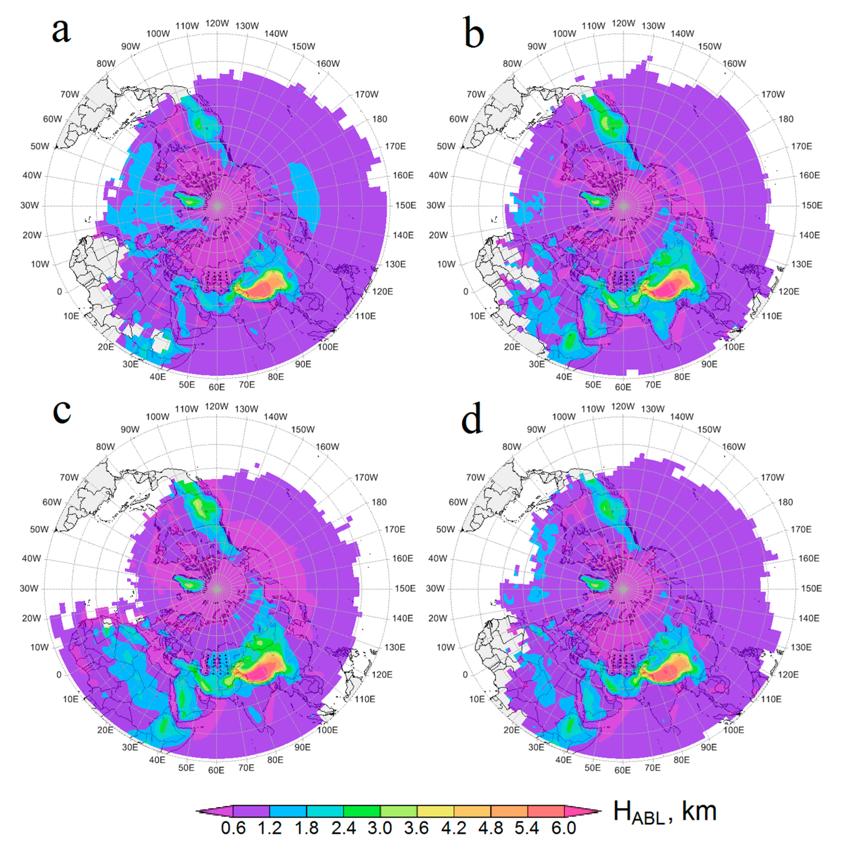
2.9. The Estimation of Average Travel Time, Average Transfer Altitude, and Average Relative Humidity in the Dust Transport Area

The mean seasonal fields T_ij, h_ij, and r_ij were reconstructed by simple averaging of the air particle flight time from the starting point to [ij] cell, the altitude of the air particle over [ij], and the relative humidity of air above [ij] cell over all FTs that crossed [ij], respectively. The averages are displayed only for the [ij] cells crossed with ≥1FTs.

3. Results and Discussion

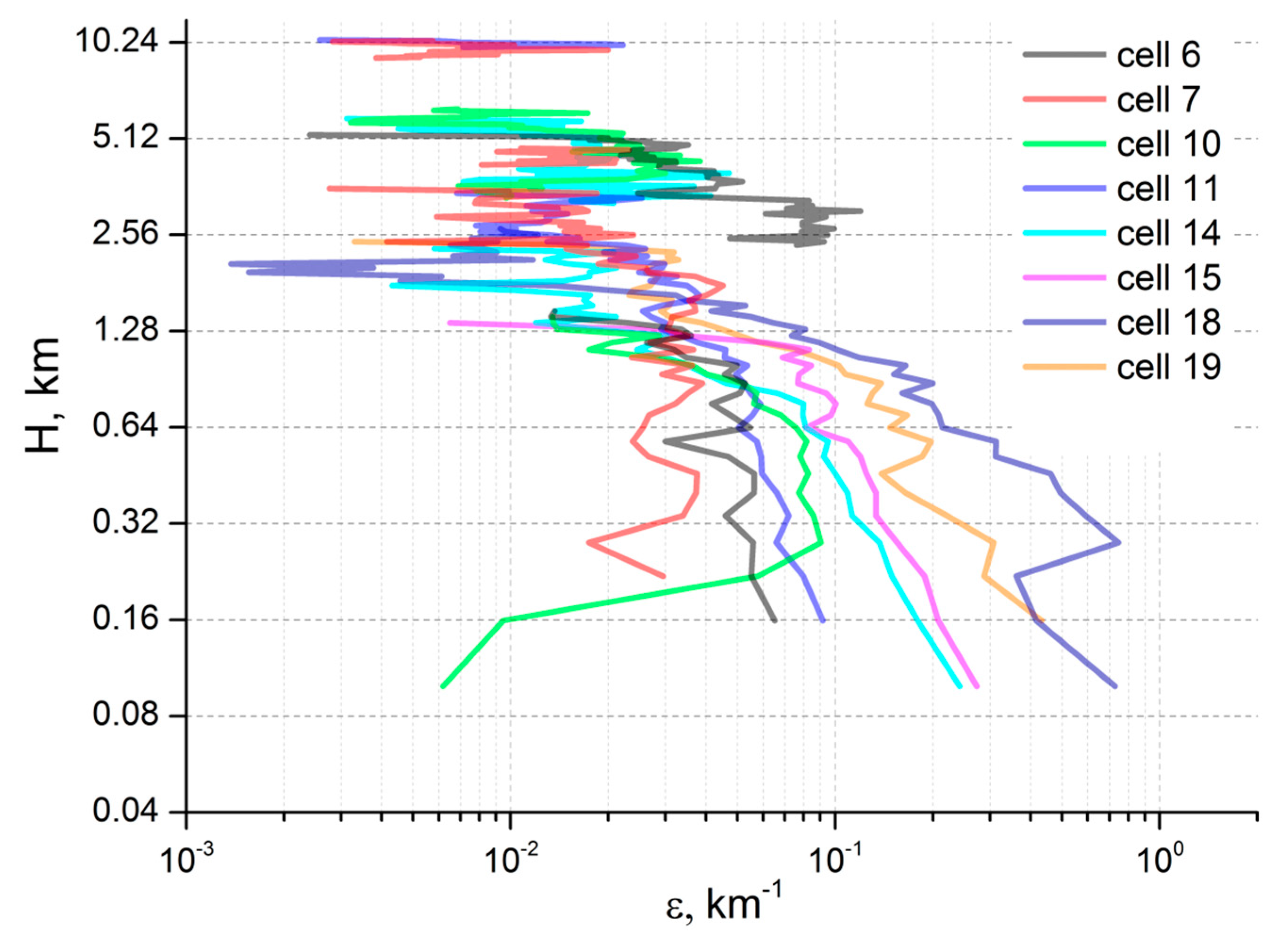
3.1. The Vertical Profiles of the Tropospheric Dust Extinction Coefficient in ACAR

The average seasonal profiles of dust ε in 2006−2021 for all ACAR cells are shown in Figure 2. The lower boundary of the profiles for different cells depends on the average cell’s surface elevation and increases from 40 m (the lower boundary of profile recovery) for the Caspian cells (1, 5, 9, 13, 17, and 21; see Figure 1) to 200–300 m near the eastern boundary of ACAR. Note that in the mountainous southeastern part of ACAR (see Figure 1), where northern Afghanistan borders Turkmenistan, Uzbekistan, and Tajikistan (cell 4; “Afghan cell”), as well as in cells 2 (north of Iranian Highlands), the average height is rather arbitrary because of the rugged relief there. In addition, the average seasonal elevations (m ASL) of the ML upper boundary, obtained by summing H from Table A2 in Appendix A and the surface elevation, are shown. As can be seen from Figure 2, the dust content in ML over some cells depends non-univocally on the season and the geographic location of the cell, as it is determined by many factors, including the type of underlying surface, seasonality of wind impact and precipitation, and the type of prevailing atmospheric circulation. For example, the dust content in ML in summer is minimal over the northern Caspian (cells 13, 17, and 21 in Figure 1 and Figure 2), when the Caspian spur of the Azores High is located above the west of the sea [141], which contributes to the transport of more clean air from the upper troposphere and/or from more northerly (and thus less arid) latitudes. At the same time, the south of ACAR is affected by the summer Iranian-Afghan minimum [141]. According to [142,143], strong dust storms on the Iranian−Afghan border in the Sistan Region are associated with an anticyclone over the northern Caspian, which probably contributes to the intensification of northern winds, as well as an increase in dust content in ML in the south of ACAR (cells 1–8 in Figure 1 and Figure 2). According to [60], this anticyclone, combined with frequent baric depression in southern Afghanistan, favors an increase in surface wind at the north of Iran and Afghanistan (i.e., in south ACAR). A detailed analysis of the factors that determine the seasonal and spatial variability of dust ε profiles is beyond the scope of this article.

The maximum average ε in ACAR were observed in spring in SL in cells 14–15–18–19 (“Aral cells”), within which the entire remains of the Aral Sea and Aralkum Desert are located, as well as the northern Kyzylkum Desert (cell 15) and most of the Ustyurt Plateau (cells 14 and 18). Large near-surface values of ε were probably determined by the high density of dust emission hotspots in the south and east of the Aralkum Desert [63]. For neighboring cells 20 and 16, and 10 and 11, far to the east and south of the Aralkum Desert, the dust emissions in spring were much lower. Note that in all seasons (except winter) in the southeast of the Ustyurt Plateau (cell 10), dust ε increased with the height decreasing up to the surface, which indicates dust emission and is consistent with the conclusions of [63] about a significant amount of sources of dust emissions in this cell near the Sarygamysh Lake.

We also note the high autumn and winter values of dust ε in the surface layer of the Afghan cell. In the north of Afghanistan (the Balkh Province), in the upper part of the Amu Darya River, there is a sandy-argillaceous southeastern spur in the Karakum Desert and, to the south of the Afghan cell (i.e., outside the ACAR), alluvial deposits in the estuary of the Balkh River, where, according to [63], the density of dusty hotspots is very high. This region is a source of dust storms; in autumn these are especially strong (due to orography) in west Tajikistan, and are known there as “Afghanets” (means “Afghan” in Russian; see [69]). Apparently, in the last two decades, Afghanets dust storms have become frequent in the winter season as well.

3.2. The Spatial Variability of Dust Optical Depth in the ACAR

The CALIOP DOD for ACAR in the layer of ≤5.02 km (lower troposphere), DOD_LT, in different seasons (see Figure 3a,d,g,j) was in good agreement with the DOD estimates for the entire atmospheric column obtained earlier for this region (see, for example, [88]). The average DOD_LT in the ACAR was ~0.022 (winter), ~0.059 (spring), ~0.055 (summer), and ~0.047 (autumn). In general, in all seasons, with the increase in ACAR latitude, DOD_LT decreased; near the southern and northern boundaries of ACAR, DOD_LT differed significantly, and the greatest zonal contrast was typical for summer and autumn. The maximum average DOD_LT values in winter (0.06), spring (0.15), summer, and autumn (0.2) were observed near the southern border of ACAR in the range of 37–39°N. Taking into account the standard deviation of DOD, which was close to 100% on average for all seasons for ACAR, the maximum DOD_LT with a high probability reached twice the average values, ~0.4 (summer and autumn), ~0.3 (spring), and ~0.1 (winter).

The average DOD_LT over four dusty (estimated using the corresponding dust ε profiles in Figure 2) Aral cells was ~0.011 (winter), ~0.069 (spring), ~0.035 (summer), and ~0.035 (autumn). Thus, considering only DOD_LT (almost equal to the DOD of the troposphere), we conclude that only in spring does the Aralkum Desert surface emit more dust than the average for the entire ACAR (see the average DOD_LT for ACAR in the previous paragraph). At the same time, cell 1 appears to have the most dust in spring, while most of the cell’s area is occupied by the Caspian Sea surface (see Figure 1). In fact, when considering the seasonal share of DOD_LT attributable only to ML over ACAR (α [%]; see Figure 3b,e,h,k), it turns out that the average α for the Aral cells of the Aralkum Desert was 38% (in winter), 57% (in spring), 56% (summer), and 44% (autumn). At the same time, the average α for the entire ACAR was 35% (in winter), 37% (in spring), 38% (in summer), and 32% (in autumn). This means that in all seasons, the relative dust content of the Aralkum Desert’s ML was higher than over the entire ACAR. We also note that in all seasons, the transit layer contained a significant amount of lower tropospheric dust: 59% (in autumn-winter) and 43% (in spring-summer), which, apparently, masked the dust-emitting cells of ACAR. As for cell 1, its ML contained only 10–15% of the lower tropospheric dust (Figure 3k), i.e., the high DOD_LT values in this cell (Figure 3j) were 85–90% because of the transport of dust clouds in the transit layer over the cell from sources apparently outside ACAR.

When considering parameter β (the proportion of DOD_LT in the lower 200 m AGL), for the Aral cells, the average β was ~37% (in winter), ~37% (spring), ~29% (summer), and ~28% (autumn). At the same time, the average β for the entire ACAR in the same seasons was ~34%, ~17%, ~13%, and ~19%. In other words, when considering thinner layers of the ACAR lower troposphere, the contrast between the dust emitting cells and the whole ACAR increased, which is reflected in Figure 3. The layer-by-layer analysis of DOD showed that in all seasons, ML and SL over the Aralkum Desert were dustier on average than the layers over the entire ACAR, i.e., apparently there is an almost year-round average dust emissions from the surface of the Aralkum Desert. This is consistent with the conclusions of [60], where modeling of the dust emissions in Central Asia for one year (March 2015–March 2016) revealed that the Aralkum Desert likely generated dust in all of the seasons. It should be noted that in almost all seasons, in most ACAR cells β > β’, and in spring and summer in the southeast of the Aralkum Desert (cell 15), these differed multiple times. In Figure 3, non-emitting (on average) dust cells are marked with an asterisk; cells are shaded where H < 200 m (i.e., non-applicable for the calculation of the β’ parameter).

In winter, the maximum DOD_LT values were realized near the southern border of ACAR, over the Afghan cell and over the south of Turkmenistan (cells 3–4). At the same time, α and β were higher in cell 4 than in cell 3, which indicates a greater dust emitting surface in cell 4, which was probably the source of dust for ML and for the lower troposphere above both cells.

In spring, DOD_LT was at a maximum over all of the cells of the southern Caspian (1, 5 and 9); however, α was minimal in this part of ACAR, i.e., the vast majority of dust was in the transition layer over the cells. It is most likely that the large DOD_LT values in spring over the southern Caspian were due to transport from distant sources. Given the prevailing eastward winds in the region during this season (see [55,138]), these sources were likely to be from the deserts of the Middle East.

In summer, the lower troposphere was maximally dusty above the Afghan cell, and the second highest DOD_LT value occurred on the south of the Caspian Sea (cell 1). At the same time, most of the dust was related to the transit layer over it, possibly for the same reason as in spring (transport from distant sources above the ML). By estimating the values of α and β, which did not have a maximum above the Afghan cell, the large DOD_LT above it could be associated with dust sources south of the Afghan cell, where most of the southeastern spur of the Karakum Desert and Balkh River’s estuary are located.

In autumn, DOD_LT was maximal over the Afghan cell. There were also local maxima for α and β, which indicates dust emissions from the surface in cell 4 and possibly to the south of it (in the Balkh River’s estuary), which were associated with the Afghanets dust storms at this time of year [69]. According to [60], dust emission within the Afghan cell occurred in all seasons, but maximum dust emissions (as well as modeled DOD) were related to spring and summer.

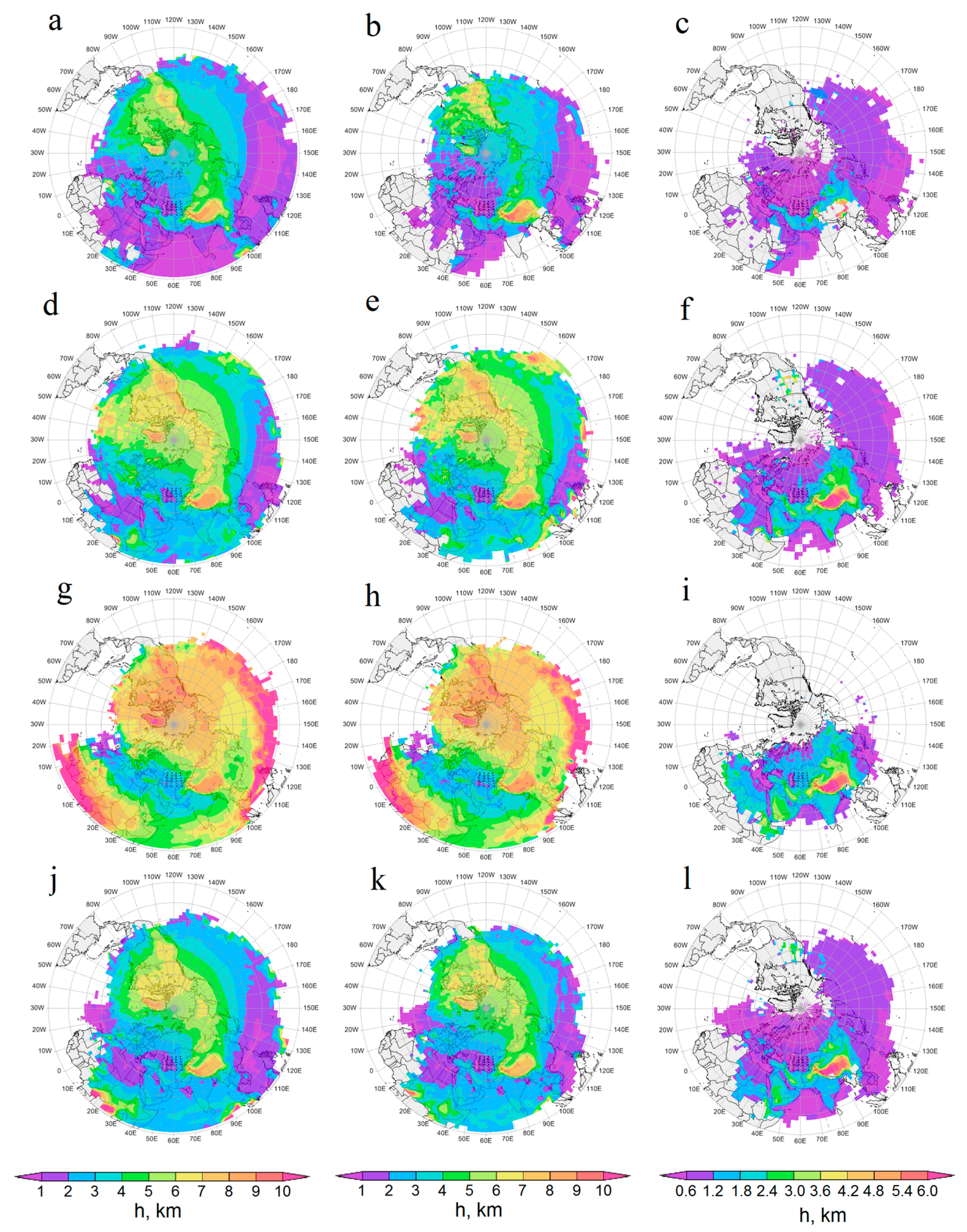
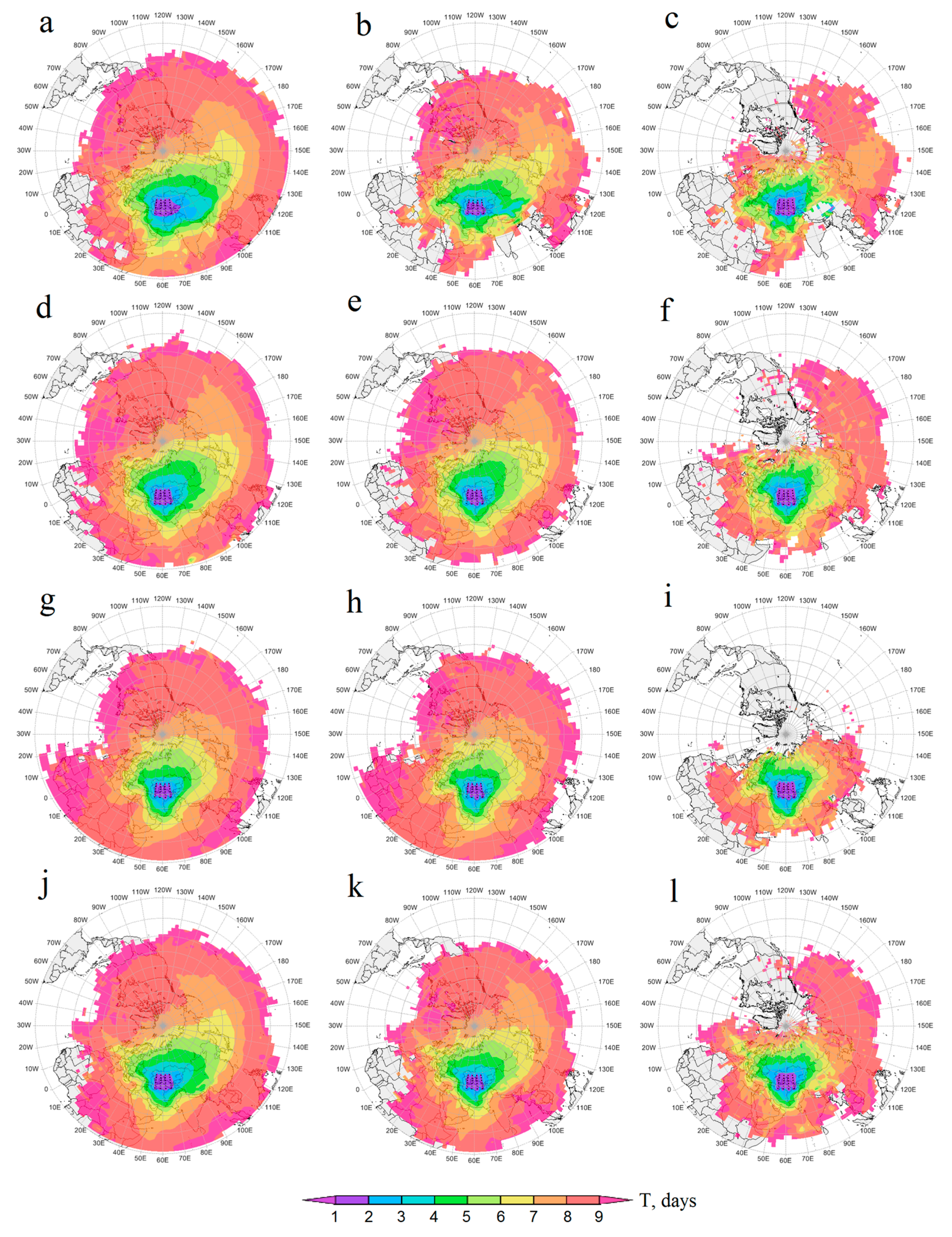
3.3. The Average Seasonal Repeatability of Air Transport from ACAR to Remote Areas

In total, ~1.01 million FTs were simulated, of which ~400,000 started in the emission layer, with the rest from the transit layer. Figure 4 displays the fields for the average seasonal repeatability of air particle transport, F [days/season], from ACAR as a whole. Everywhere below, when mentioning a geographical region, indicates parts located in the Northern Hemisphere. Depending on the season, the maximum achievable F is in the range of 90–92 days/season; if F < 1, the air transport did not happen every year. For convenience, we denoted the repeatability of ≥64 days/season as almost daily, with 32–63 meaning very often, 16–31 often, 8–15 non-rarely, 1–7 rarely, and <1 not every year. In

Table 1. Seasonal repeatability [days/season] of air transport from the layers of the ACAR lower troposphere to the troposphere in some control areas of the Northern Hemisphere. Here and after in the tables, seasons are marked as follows: I—winter (DJF), II—spring (MAM), III—summer (JJA), and IV—autumn (SON). The following repeatability ranges are highlighted in color: ≥64 (dark red), 32–63 (red), 16–31 (orange), 8–15 (yellow), 1–7 (green), and <1 (blue).

Site	$\mathbf{ACAR}’\mathbf{s} \mathbf{Low} \mathbf{Troposphere} \Rightarrow$ Regional Troposphere				$\mathbf{ACAR}’\mathbf{s} \mathbf{Dust} \mathbf{Transit} \mathbf{layer} \Rightarrow$ Regional Troposphere				$\mathbf{ACAR}’\mathbf{s} \mathbf{Dust} \mathbf{Emission} \mathbf{Layer} \Rightarrow$ Regional Troposphere
	I	II	III	IV	I	II	III	IV	I	II	III	IV
Moscow region	23	23	23	24	20	18	16	19	11	18	19	18
Volga region	39	42	37	38	36	35	29	32	19	32	30	29
Southern Urals	52	53	49	49	48	46	38	42	25	41	41	36
South-western Siberia	59	63	62	61	57	56	51	55	25	48	52	44
Baikal Region	56	63	65	65	54	56	55	60	19	46	53	44
Amur Region	42	55	56	61	40	48	45	55	14	38	42	38
Prymorie region	53	66	57	70	52	59	46	66	16	45	41	42
Black Sea−Caspian	28	34	44	35	24	27	35	27	18	27	37	29
Northwest Russia	25	22	23	24	23	17	17	19	11	16	19	18
Northern Urals	39	39	35	36	36	31	27	29	17	30	29	27
West Siberia	45	44	46	46	41	36	35	38	20	34	38	34
Yakutia	30	42	50	44	28	34	38	37	10	29	38	27
Chukotka	24	31	30	38	23	25	21	34	3	16	21	16
Barents Sea	18	16	14	17	16	11	9	12	6	11	11	11
Kara Sea	27	25	23	26	25	18	16	20	10	18	18	17
Laptev Sea	25	29	30	31	23	22	21	25	7	19	23	19
East Siberian Sea	20	25	23	29	18	19	15	24	4	14	16	14
West Iran	7	11	38	14	6	8	27	10	3	7	30	9
East Iran	24	39	81	52	20	31	72	43	12	27	73	37
Central Iran	7	14	59	23	6	10	48	18	3	9	49	14
South Iran	5	8	58	18	4	5	47	15	1	5	47	10
West China	24	39	55	39	23	33	42	35	3	21	41	16
North India	7	18	47	19	7	14	34	16	1	10	34	6
Southeast Asia	10	8	5	9	10	7	3	8	1	4	3	2
Mesopotamia	4	6	13	5	3	4	8	3	1	4	8	3
Arabian Peninsula	2	2	20	6	2	1	14	5	<1	1	13	2
Northeast Africa	1	2	8	2	1	1	5	1	<1	1	5	1
Northwest Africa	-	<1	<1	-	<1	<1	<1	<1	-	-	<1	-
North America (USA)	11	17	9	17	10	14	6	16	1	6	4	4
East Europe (outside Russia)	6	7	7	6	5	5	5	4	2	4	6	5
West Europe	3	4	2	3	3	3	1	2	1	3	1	2
North Pole region	10	11	8	11	9	8	5	8	2	6	5	6

and

Table 2. Seasonal (I—winter, II—spring, III—summer, IV—autumn) repeatability [days/season] of air transport from the ACAR’s emission layer to the mixed layer over the selected sites of the Northern Hemisphere. The following repeatability ranges are highlighted in color:, 32–63 (red), 16–31 (orange), 8–15 (yellow), 1–7 (green), and <1 (blue).

Site	I	II	III	IV
Moscow Region	3	5	5	5
Volga Region	4	9	8	8
Southern Urals	7	10	8	9
South-western Siberia	4	8	8	8
Baikal Region	1	5	4	3
Amur Region	-	2	1	1
Prymorie Region	2	2	<1	4
Black Sea−Caspian	10	14	21	19
Northwest Russia	2	2	2	3
Northern Urals	2	2	2	3
West Siberia	1	1	2	2
Yakutia	-	-	1	1
Chukotka	-	-	-	-
Barents Sea	3	1	<1	-
Kara Sea	1	1	-	1
Laptev Sea	<1	<1	-	1
East Siberian Sea	<1	-	-	<1
West Iran	2	4	19	6
East Iran	8	22	63	30
Central Iran	2	7	38	11
South Iran	1	3	23	6
West China	1	7	19	5
North India	<1	6	10	3
Southeast Asia	<1	1	-	1
Mesopotamia	1	2	5	2
Arabian Peninsula	-	1	7	2
Northeast Africa	<1	1	3	1
Northwest Africa	-	-	-	-
North America (USA)	-	-	-	-
East Europe (outside Russia)	1	1	1	2
West Europe	<1	<1	-	1
North Pole Region	-	-	-	-

, the values of F are given for a number of small control sites, whose titles reflect the geographical region where the sites are located. The boundaries of these regions are given in

Table A3. Titles, latitudes, and longitudes of the control sites used for estimating the mean seasonal repeatability of the air transport from ACAR. Each site is titled as the geographical region where the area is included.

Site	Latitude Range	Longitude Range
Moscow region	53N … 58N	32E … 42E
Volga region	53N … 58N	47E … 57E
Southern Urals	55N … 60N	65E … 75E
South-Western Siberia	53N … 58N	80E … 90E
Baikal region	52N … 57N	105E … 115E
Amur region	54N … 59N	125E … 135E
Prymorie region	44N … 50N	135E … 140E
Black Sea−Caspian	44N … 50N	40E … 46E
Northwest Russia	62N … 67N	35E … 55E
Northern Urals	63N … 68N	65E … 75E
West Siberia	63N … 68N	80E … 90E
Yakutia	63N … 68N	120E … 140E
Chukotka	63N … 68N	170E … 180E
Barents Sea	73N … 78N	35E … 55E
Kara Sea	73N … 78N	65E … 95E
Laptev Sea	73N … 78N	105E … 140E
East Siberian Sea	73N … 78N	150E … 180E
West Iran	34N … 39N	45E … 50E
East Iran	34N … 38N	53E … 60E
Central Iran	30N … 34N	48E … 60E
South Iran	26N … 30N	50E … 60E
West China	35N … 41N	78E … 88E
North India	23N … 28N	73E … 80E
Southeast Asia	10N … 30N	100E … 120E
Mesopotamia	31N … 36N	35E … 45E
Arabian Peninsula	22N … 27N	42E … 47E
Northeast Africa	20N … 30N	20E … 30E
Northwest Africa	20N … 30N	10W… 0E
North America (USA)	43N … 53N	95W … 115W
East Europe (outside Russia)	42N … 52N	14E … 24E
West Europe	42N … 52N	0E … 10E
North Pole region	80N … 90N	180W … 180E

in Appendix A. The seasonal patterns of transport from the ACAR lower troposphere (ACAR-LT), from the ACAR dust transit layer (ACAR-TL), and from the ACAR dust emission layer (ACAR-EL) were similar to each other. At the same time, they were all very different from the corresponding seasonal patterns of transport from ACAR-EL to the regional mixed layer, so this case is analyzed in a separate Section 3.3.2. On the territory of ACAR itself, F (as DOD’) could be reconstructed incorrectly, thus the ACAR values of F were not analyzed.

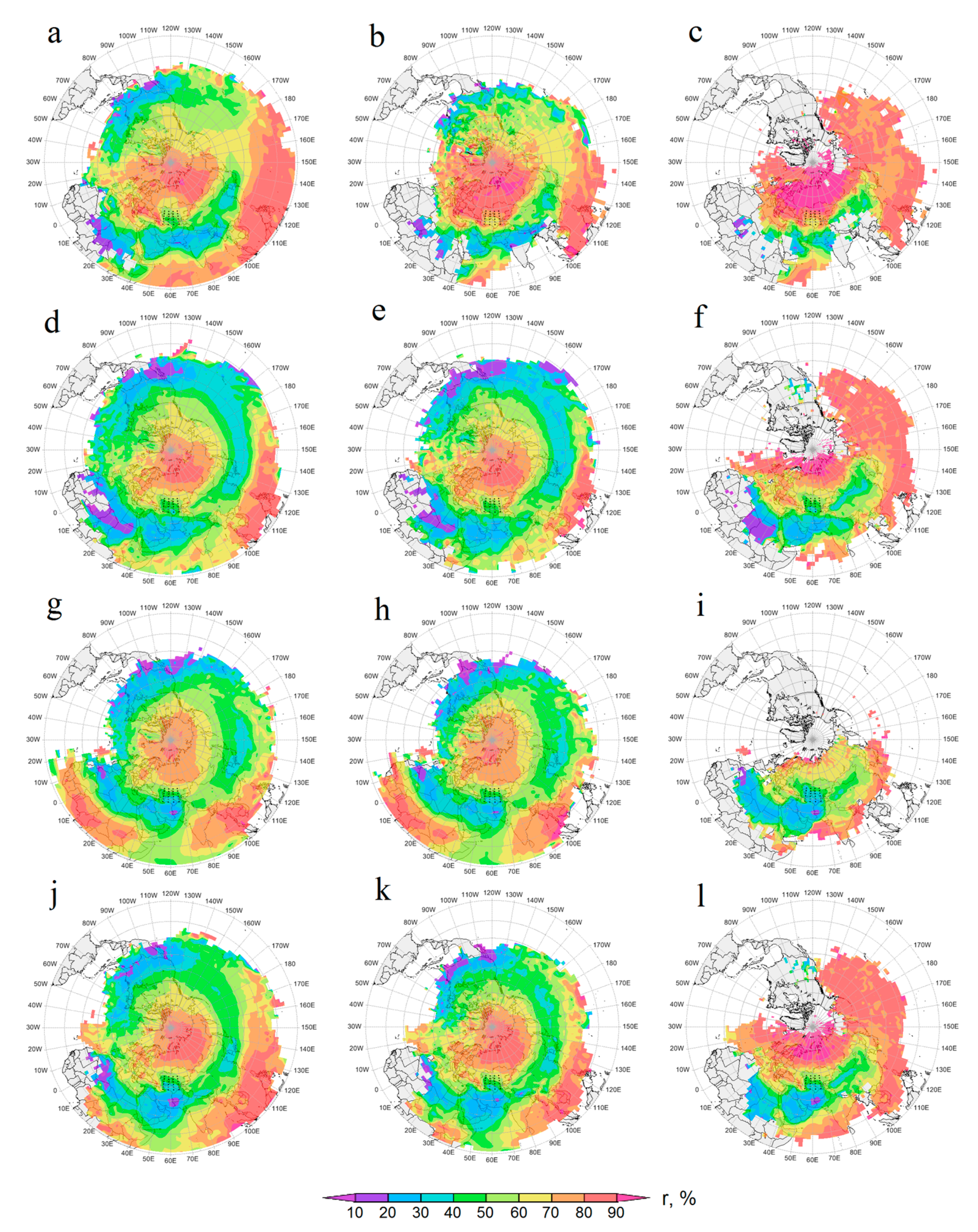
3.3.1. The Repeatability of Air Transport from the ACAR Lower Troposphere Layers

In general, air transport from the entire ACAR-LT (Figure 4a,e,l,m) was due to large-scale atmospheric circulation, which is formed by the permanent and seasonal atmospheric centers of action in the Northern Hemisphere, polar vortex, Icelandic Low, Siberian (Asian) and Azores Highs, etc., as well as synoptic scale eddies, cyclones, and anticyclones. Together, they cause a very complex configuration both of individual FT and the patterns of air transport from the ACAR as a whole. Consequently, in all seasons, air from ACAR spread for 10 days over most of the Northern Hemisphere (see Figure 4). The long range of air particle propagation was facilitated by a rapid increase in the transport height east of the ACAR to the altitudes above the lower troposphere (see Figure A2 in Appendix A), where the influence of the polar vortex dominated for most of the year. According to [50,93], in May 2007, dusty air in the immediate vicinity of ACAR (Tian Shan Mountains) ascended up to the tropopause, where the dust cloud was carried away by the polar jet stream and, according to [134], performed one full circuit in 13 days around a globe in the Northern Hemisphere. The authors of [41] explained the spring and winter rise of dust from North Africa and the Arabian Peninsula to the upper troposphere during dust eastward transport by the influence of mountain systems in the west of Central Asia. ACAR is closer to these mountains than the Middle Eastern and African dust sources, so this lifting mechanism was probably likely for ACAR dust as well. As can be seen from Figure A2 in Appendix A, in all seasons, the average transport altitude increased abruptly to 5–6 km above the mountain systems to the east (Tian Shan and Altai Mountains) and to the southeast (Pamir Mountains) of ACAR, and further east in the same latitude range the average did not decrease. Even in winter, the air that started in ACAR-EL reached altitudes of ~5 km over eastern Siberia and 6–7 km over North America. In winter, the average ML depth above ACAR was ~267 m AGL (standard deviation of 91 m) and did not exceed 600 m AGL, even over the warm southern part of the Caspian Sea (see Table A2 in Appendix A and Figure 2). In general, in winter, the average altitude in the air transport area was less than in other seasons; therefore, in this season compared with the others, the propagation distance and, accordingly, F, decreased faster as it moved further from ACAR. Unexpectedly (and currently inexplicably), regardless of the starting layer (ACAR-LT, ACAR-EL, or ACAR-TL) and direction of transport, after ~4 days, the average altitudes of air particles were approximately equal (compare Figure A2 and Figure A3 in Appendix A).

With greater or lesser repeatability, the air from all of the studied layers spread to the whole of Europe, Asia, and the Arctic, and reached North America (up to the territory of Mexico), most of the Pacific Ocean (especially in winter), and a significant part (entire in summer) of Africa, southeastern Asia, the Indian Ocean, and the North Atlantic. At the same time, for all seasons, transport to the Atlantic south of 25°N, including the region near the Caribbean Islands as well as to the American continent south of 20°N, was very low in probability. It can be argued that the dust from ACAR could likely not contribute significantly to the aerosol load within SAL.

Greenland occupies a special position in the air transport patterns. For all seasons, air transport to the island (especially to its southern part) from ACAR was difficult, despite Greenland’s relative proximity to the ACAR in comparison, for example, with North America. Air transport along the shortest northwestern (through Europe) or northern (through the Barents Sea) route was relatively rare on average, even in summer (when meridional air transport was most likely) due to the dominance of westerly winds in the mid-latitudes of the Northern Hemisphere. The eastward transport (through Asia, the Pacific Ocean, and North America) seemed to last longer than 10 days on average (see Figure A3 in Appendix A), so only the fastest and rarest (as in the case described in [134]) air particles could reach Greenland via this route. Based on 7-day trajectories for 131 dust episodes over Japan in 2001–2010, the authors of [52] identified the route of dust transport from Central Asia to the Arctic through the Chukchi Sea. From [51], it can be seen that this route can cross the Arctic Ocean and reach the Nunavut Region of Arctic Canada in the immediate vicinity of Greenland. It is possible that dust from the Taklimakan Desert identified in the Greenland aerosol samples [57] and possibly dust from the ACAR entered the air over island in this way.

For all of the seasons, the dominance of eastward air transport in the Northern Hemisphere mid-latitudes (where most of ACAR is located) determined the highest F for the territories to the east and southeast of ACAR. The repeatability patterns for the transport from ACAR’s lower troposphere were qualitatively similar to the results from [55] for the seasonal horizontal dust flux in the troposphere throughout Central Asia, which is dominantly eastward in winter, spring, and autumn, and mainly southward in summer due to the influence of the eastern periphery of the Caspian anticyclone, where the air moves from north to south.

In winter, the zone of almost daily air transport from ACAR’s lower troposphere (see Figure 4a) was the least compared with in other seasons (see Figure 4f,i,m), possibly due to the collision of the dominant eastward airflow over central Eurasia driven by the Icelandic Low and the polar vortex (strongest in this season) and oncoming air currents generated at the southwestern periphery of the Asian (Siberian) anticyclone, which was also maximum in winter. The superposition of these factors, probably, also determined the minimum area of the zone of frequent and very frequent air transport from ACAR-EL (Figure 4c), which only reached the Japan Islands in winter, while in other seasons it extended up to the western coast of North America (Figure 4g,k,o). Generally, in winter, air transport from the entire ACAR lower troposphere was determined by transport from ACAR-TL (Figure 4b).

In the transitional seasons (Figure 4e,m), when the Siberian anticyclone weakened (in spring) or only intensified (in autumn), the zone of almost daily air transport from the ACAR lower troposphere extended maximally to the east, reaching the Pacific Ocean south of the Aleutian Islands in a latitude range of 30–50°N in spring (Figure 4e) and 40–50°N in autumn (Figure 4m). During these seasons, air masses from ACAR’s lower troposphere were often reached, even the central regions of North America. The contribution of the air transport from ACAR-EL to the air transport from the entire ACAR lower troposphere in spring and autumn was much higher than in winter.

In summer (Figure 4d), the contribution of air transport from ACAR-EL to the air transport from the entire lower troposphere of ACAR was maximal, as the average ML depth above ACAR was the highest. In this season, the meridional component of air transport intensified due to a decrease in the zonal temperature contrast in the Northern Hemisphere and, as a result, a weakening in the polar vortex. In ACAR, this meridional component was driven, probably, by the eastern spur of the Azores High. Regardless of FT’s starting layer, air particles moving to the west of the ACAR were, on average, at a much lower altitude (2–3 km) than for FTs moving to the east (Figure A2i–k; see Appendix A). At the same time, the zone of almost daily air transport bifurcated into the eastern spur, reaching only the eastern border of Mongolia, and the southern spur, extending to the Arabian Sea.

For all of the seasons, the air from ACAR’s lower troposphere was often or very often transported to almost the entire territory of Russia (see Table 1 and Figure 4). The zone of almost daily air transport covered the Baikal Region (in summer and autumn) and Primorye Region (in spring and autumn). During the entire year, the air transport was repeated very often or often over the Urals; western Siberia; the Amur, Baikal, and Primorye Regions; and the Black Sea−Caspian Region of Russia. In every season, the densely populated north-west of the Russian Federation, including the Moscow Region, as well as the Kara, Laptev, and East Siberian Seas, were often exposed to air intrusions from ACAR.

In summer, the air transport was repeated very often to the entire territory of Iran, and almost daily to the east and south of the country. Thermal low-pressure systems over low topographic areas and the high-pressure Caspian Sea, along with intense surface winds over the dust sources caused the dust outbreaks and transport over Iran in summer [145]. Many dust storms in west, SW, and NW Iran were driven by the Shamal wind in summer [146] and frontal system in winter [147,148,149]. In other seasons, the east (Khorasan Province) and west (Western Azerbaijan Province; see [145]) of Iran were very often subject to the influence of ACAR air.

3.3.2. The Repeatability of Air Transport from ACAR to the Regional Atmospheric Mixed Layer

The duration and range of propagation of air particles in ML (as part of ABL) were strongly influenced by ML depth, as well as synoptic-scale eddies, cyclones, and anticyclones. The former contributed to the movement of air particles from ABL into the free troposphere, i.e., a decrease in the transport distance in ML, and the latter, on the contrary, favored the preservation of an air particle in ABL, i.e., an increase in the air transport area within ABL. In this section, we discussed the recurrence of the transport of air particles that started in the ACAR-EL and moved into the ML outside ACAR. In this case, the same air particle in some regions could move into ML (and would be taken into account in them) in others regions it could move above ML (it would not be taken into account).

In winter, the only zone of often air transport from ACAR-EL to regional ML was located over the Caspian Sea (Figure 4d). In this season, the transport was repeated non-rarely to ML over the Russian Black Sea and Caspian territories, as well as over the northeast of Kazakhstan and the northeast of Iran. The dominant wind direction was southwesterly over the Urmia Lake and NW Iran [138,150], so saline dust from the dried lake bed mostly affected the Caspian Sea area. For most of the European territory of Russia (ETR) and the Barents Sea, the transport was non-rare. Over western Siberia and Mongolia, there was a zone of rare or non-annual transport. The decrease in F for these regions could be explained by the presence of a barrier to the movement of air particles in ML in the form of counter descending air flows on the western and southwestern periphery of the Siberian (Asian) High. In addition, under the conditions of the winter anticyclone, ML could decrease even in the daytime, until its disappearance [116]. From the east coast of China, the zone of often transported from ACAR-EL to the regional ML again started extending to almost 180°E (Figure 4d). This area, apparently, was formed by those air particles that started in the ACAR-EL and passed around the air barrier over western Siberia and Mongolia, moving either much higher or to the south of it. The average altitude of air particle transport from ACAR-EL (see Figure A2d in Appendix A) over western Siberia and Mongolia was ~4 km but over the Pacific Ocean, east of the Japan Islands, it was ~1.5 km, while in winter, the average ML depth in this transport area was also ~1.5 km (see Figure A5 in Appendix A). It should be noted that according to [97], in February 2009, samples of surface layer aerosols in Japan included Central Asian dust from the territories east of Japan. Based on the analysis of 3-day backward trajectories, this dust was associated with transport from Mongolia (Gobi Desert), although the use of longer trajectories could indicate more western dust sources.

During the transitional seasons (Figure 4h,p), patterns of this type of air transport had many common features. The zone of often transported extended to the Caspian territories of Russia, the north-west of Kazakhstan (outside the ACAR), and almost the entire east of Iran. In spring and autumn, the transport repeated non-rarely to the southern Volga region and the southern Urals, as well as northwestern China, Pakistan, and Afghanistan. In spring, in contrast with autumn, transport to Mongolia and northern India was non-rare. The transport was rare to the ML of the Moscow Region, as well as to the northwestern and western regions of the Russian Federation and most of the Asian territory of Russia (ATR). ML over the Russian Arctic Seas was intruded as non-annual with air from ACAR-EL.

The summer bifurcation of the zone of maximal F into the eastern and southern spurs manifested itself in the patterns of F for the regional ML (Figure 4h). During this season, transport to the Black Sea and Caspian territories of Russia was realized often; for the rest of the Russian territory, the transport pattern was the same as for the transitional seasons. Air transport to the greater territory of Kazakhstan (outside the ACAR) and northwest China also happened often. The highest F was characteristic for ML throughout the territory of Iran, to which ACAR-EL air was transported very often, while to the north-east of the country (to Khorasan Province) it was almost daily.

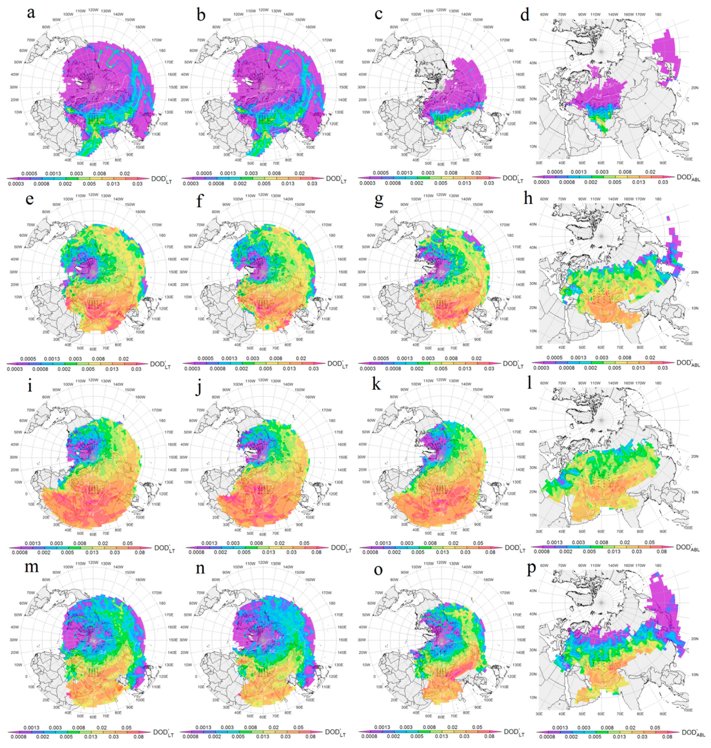
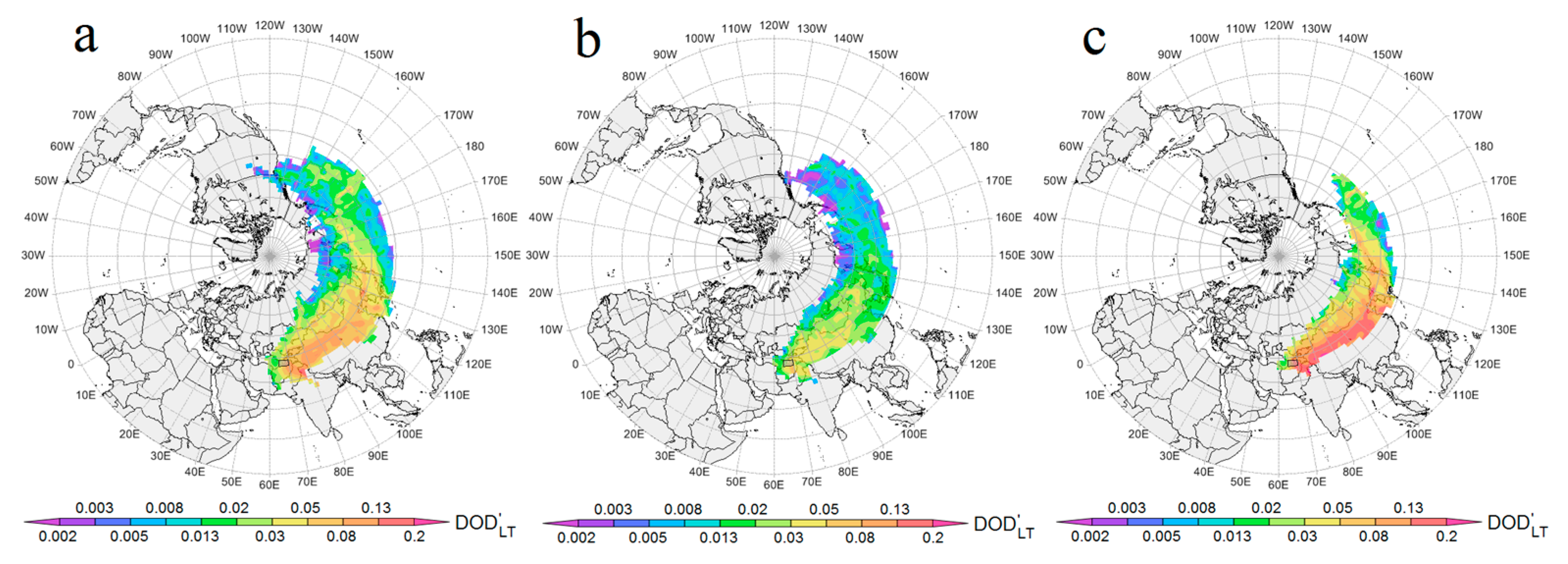
3.4. Potential Impact of the ACAR Dust on Regional DOD

Figure 5 displays the average seasonal contribution of ACAR’s dust emission layer to the regional tropospheric DOD, DOD’_LT, (the first column from the left), the average seasonal contribution of the ACAR’s dust transit layer to DOD’_LT (the second one), and the ACAR’s dust emission layer to DOD’_LT, (the third one), as well as the average seasonal contribution of ACAR-EL to the DOD of the regional ML outside ACAR, DOD’_ML (fourth column). Only the [ij] cells crossed with ≥50 air particles are shown. Note that a very low (or very high) contribution to the regional DOD’ does not mean that there could not have been individual outbreaks of extremely dusty (or extremely clean) air from ACAR during this season. Seasonal mean DOD’ × 10³ (i.e., 50 represents DOD’ = 0.05) over the selected control sites (see Table A3 in Appendix A), characterizing large geographic regions of the Northern Hemisphere, are given in

Table 3. Seasonal (I—winter, II—spring, III—summer, and IV—autumn) regional dust optical depth (DOD’ × 10³) due to air transport from ACAR’s dust emission layer into the regional troposphere over the control sites. DOD’ × 10³ ranges are highlighted in color: ≥50 (red), 30–49 (orange), 10–29 (yellow), 1–9 (green), and <1 (blue). An asterisk (*) indicates statistically insignificant DODs.

Site	$\mathbf{ACAR}’\mathbf{s} \mathbf{Low} \mathbf{Troposphere} \Rightarrow$ Regional Troposphere				$\mathbf{ACAR}’\mathbf{s} \mathbf{Low} \mathbf{Troposphere} \Rightarrow$ Regional Troposphere				$\mathbf{ACAR}’\mathbf{s} \mathbf{Low} \mathbf{Troposphere} \Rightarrow$ Regional Troposphere
	I	II	III	IV	I	II	III	IV	I	II	III	IV
Moscow Region	<1	11	29	10	<1	13	34	10	<1	8	23	9
Volga region	1	13	32	11	1	13	38	6	1	11	22	14
Southern Urals	<1	15	22	7	<1	17	24	6	<1	10	20	8
South-western Siberia	1	10	16	8	1	8	16	5	1	12	16	12
Baikal Region	<1	7	16	9	<1	6	16	6	<1	7	16	15
Amur Region	1	4	13	4	<1	4	12	3	<1	3	14	5
Prymorie Region	<1	5	19	8	<1	5	15	7	<1	5	23	13
Black Sea−Caspian	1	16	52	18	<1	19	71	15	1	11	36	21
Northwest Russia	<1	6	22	4	<1	7	27	4	<1	4	17	4
Northern Urals	<1	7	15	5	<1	8	17	6	<1	5	15	5
West Siberia	<1	6	10	3	<1	6	10	2	<1	6	10	4
Yakutia	<1	4	12	4	<1	4	13	4	<1	4	12	5
Chukotka	<1	2	8	1	<1	2	6	1	<1	3	9	1
Barents Sea	<1	2	14	3	<1	2	13	3	<1	2	12	3
Kara Sea	<1	4	11	2	<1	4	13	2	<1	3	11	2
Laptev Sea	<1	3	11	2	<1	3	12	2	<1	3	9	2
East Siberian Sea	<1	3	9	4	<1	3	11	2	<1	2	7	7
West Iran	2	23	76	33	1	26	83	27	3	20	65	37
East Iran	4	35	71	37	2	41	77	33	7	29	65	45
Central Iran	3	28	67	39	3	29	75	35	5	26	54	44
South Iran	2	28	103	43	2	22	99	36	4	32	105	51
West China	2	25	58	49	2	25	50	28	5 *	25	64	107
North India	1	30	65	20	<1	14	63	16	<1 *	37	69	31
Southeast Asia	3	14	36	17	3	13	36	15	4 *	16	37	30
Mesopotamia	<1	8	68	21	<1	10	75	19	1 *	6	47	19
Arabian Peninsula	1	4	61	48	1	1	53	36	<1 *	7 *	62	64
Northeast Africa	1 *	30 *	71	22	1	13	98	13	1 *	38 *	47	27 *
Northwest Africa	<1 *	8 *	12 *	9 *	-	6	4	<1	<1 *	10 *	13 *	9 *
North America (USA)	<1	3	6	3	<1	2	6	2	<1 *	3	6	10
East Europe (outside Russia)	2	7	26	20	2	6	39	34	1 *	8	17	7
West Europe	1	9	12 *	11	<1	10	22	23	<1 *	7	7 *	3
North Pole Region	<1	1	7	4	<1	2	7	2	<1 *	1	6	4

(for 1one to three types of transport) and in

Table 4. Seasonal regional dust optical depth (DOD’ × 10³) due to air transport from the ACAR dust emission layer into the mixed layer over the control sites. DOD’ × 10³ ranges are highlighted in color: ≥50 (red), 30–49 (orange), 10–29 (yellow), 1–9 (green), and <1 (blue). An asterisk (*) indicates statistically insignificant DOD.

Site	I	II	III	IV
Moscow Region	<1 *	5	13	6
Volga Region	<1	5	8	2
Southern Urals	<1	7	12	4
South-western Siberia	<1 *	4	9	5
Baikal Region	<1 *	4 *	11 *	5 *
Amur Region	<1 *	<1	4 *	<1 *
Prymorie Region	<1 *	2 *	4 *	1 *
Black Sea−Caspian	<1	6	15	7
Northwest Russia	<1 *	3 *	9	1
Northern Urals	<1	1	5	1
West Siberia	<1 *	<1 *	8 *	1 *
Yakutia	<1 *	1 *	3 *	<1 *
Chukotka	<1 *	<1 *	<1 *	<1 *
Barents Sea	<1	<1 *	<1 *	<1 *
Kara Sea	<1 *	<1 *	2 *	<1 *
Laptev Sea	<1 *	<1 *	3 *	<1 *
East Siberian Sea	<1 *	<1 *	<1 *	<1 *
West Iran	3 *	19	33	41
East Iran	6	20	38	38
Central Iran	3 *	19	43	44
South Iran	3 *	17	39	38
West China	<1 *	13	59	73
North India	<1 *	17	26	24
Southeast Asia	4 *	6 *	22 *	11 *
Mesopotamia	1 *	7	23	15
Arabian Peninsula	<1 *	11 *	23	45 *
Northeast Africa	1 *	35 *	49	8 *
Northwest Africa	<1 *	3 *	7 *	6 *
North America (USA)	<1 *	<1 *	<1 *	<1 *
East Europe (outside Russia)	<1 *	5	8	8
West Europe	<1 *	<1 *	<1 *	1 *
North Pole Region	<1 *	<1 *	<1 *	<1 *

(for transport of type 4). An asterisk indicates DOD’ values for the sites where all or most of the [ij] cells were crossed with <50 air particles.

As shown above, in spring, summer, and autumn, ACAR-EL and ACAR-TL each contained (in average by entire ACAR) 45–55% of tropospheric dust (see Section 3.2), and far away from ACAR, air transport from both its layers occurred, on average, at approximately the same altitudes (see Figure A2 in Appendix A). This led to an approximately equal contribution of both layers to DOD’_LT for most remote regions, so over them, the impact of the two layers was not summed, but averaged. DOD’_LT for the region adjoined immediately to ACAR was most dependent on the DOD of ACAR cells that were the nearest to the region.

3.4.1. The Potential Impact of the ACAR Lower Tropospheric Layers on the Regional DOD

Previously (see Section 3.2), it was found out that DOD_LT was minimal in winter, both within the entire ACAR and within its individual cells (see Figure 3a). In addition, in this season, the probability of an air particle entering the cloud layer was high near ACAR, as evidenced by the field of average r in the air transport area (see Figure A4 in Appendix A). These factors could explain the relatively low regional winter DOD_’LT, even near ACAR (Figure 5a–c), compared with other seasons. DOD’_LT reached its maximum values (0.003–0.005) south of ACAR, near the Iran−Afghan border (near Hamun Lake, which is a major source of dust storms at the eastern border of Iran), over the Arabian Sea, as well as over the Tibetan Plateau, southeast China, southern Europe, and the Balkan and Apennine Peninsulas (Figure 5a). As can be seen from the comparison in Figure 5a–c, a large air transport area over the Arabian Sea was formed by dusty air transported from ACAR-TL, while dust from ACAR-EL (i.e., dust most likely from the surface of the ACAR itself) was transported to northeast Iran (Figure 5c). Such phenomena happened before and dust emissions from the ACAR region were transported to NE Iran [145]. The transport zone from ACAR-EL was significantly smaller than that for ACAR-TL; therefore, in winter, ACAR-EL most strongly affected the surrounding territories near ACAR, in northeast Iran (0.005–0.008), Tajikistan, and Kyrgyzstan (0.008–0.013), as well as some areas in west and east China (up to 0.02).

In winter, throughout Russia, DOD’_LT ≤ 0.001, and DOD’_LT reached its maximum values (0.001) over the Caspian−Black Sea Region, the southern Volga Region, the southern Urals, and the south of western Siberia (Figure 5a–c). The dust transport to the territory of Russia was likely prevented by a barrier from the zone of high r surrounding ACAR from the north and extending over the whole of Russia (see Figure A4a–c in Appendix A). In Iran in winter, DOD’_LT reached its maximum values (~0.003) over the territories bordering Afghanistan in the Hamun Lake dust source. In the remaining territory of Iran, DOD’_LT was in the range of 0.008–0.012, excluding the Urmia Lake Region, where DOD’_LT < 0.001 in winter month.

In spring, the average ML depth in ACAR was significantly higher (see Table A2 in Appendix A), while the average r in the transport area was noticeably lower than in winter (Figure A4e–g; see Appendix A); therefore (ceteris paribus), ACAR dust could spread to larger areas. This also applied to summer and autumn dust transport patterns. In spring, F for all layers above ACAR was maximum for the zone to the east of ACAR, in the same range of latitudes (see Figure 4e–g), where ACAR itself was located. One could also expect the maximum average DOD’_LT for all layers for this zone, given that in spring, ACAR-TL contained ~43% of tropospheric dust (see Section 3.2); however, the average contribution of ACAR here was high (0.013–0.02), but not maximal (Figure 5e–g). On average, the regions located to the south in a wide latitude, ranging from the southern border of ACAR to the Mediterranean Sea in the west, the Arabian Sea in the south, and the Bay of Bengal in the southeast, were subject to the greatest potential impact from both layers of ACAR’s lower troposphere (Figure 5e–g). Apparently, in spring, a zone of high pressure started to develop over the Caspian Sea, supporting dust transport to the south of ACAR at relatively low transport altitudes. In the pointed latitudinal zone, air particles moved at altitudes in the range of 2 to 3 km for all of the layers studied (Figure A2 in Appendix A). ACAR-EL and ACAR-TL contributed approximately equally (0.02–0.03) to DOD’_LT in the northeast of Iran, Afghanistan, Tajikistan, and Kyrgyzstan. The impact of ACAR-EL extended over the territories of Pakistan (0.02–0.03) and northern India (>0.03), while ACAR-TL impacted the northwest of the Bay of Bengal more. Although in spring, the main dust transport was southward, the ACAR dust plume spread eastward as far as North America (0.002–0.005), including the Rocky Mountain Region. In some cases (see [134]), a dusty cloud moving along this route could circumnavigate the entire globe. Backward trajectory modeling for 131 dusty episodes recorded over Japan in 2001–2010 indicated transport from the arid Central Asian regions west of Japan [52]. The eastward dust transport is also confirmed by observations of dust clouds in the lower troposphere over Japan [50].

In the Russian territory, the maximum spring values of DOD’_LT (0.02–0.03) were realized in the Caspian regions (in Dagestan and Kalmykia) because of the impact of the dust transit layer (compare Figure 5a,b). The other Russian regions were affected approximately equally by both the emission and transit layers, and larger mean DOD’s were realized for ETR (0.008–0.02) than for ATR (0.002–0.008). In the Moscow Region, DOD’_LT was about 0.008. The authors of [151] found out that during the warm season (April–September), extreme volume concentrations of aerosols in the range of 2.5–5 µm (typical for dust) in the atmosphere above Moscow (according to the data of Moscow AERONET site in 2001–2018) were associated with air transport from ML over the Turan Lowland in the immediate vicinity of the Aralkum Desert. The impact of ACAR on the content of silicates (one of the markers of dust) in the surface layer samples of aerosols in the range of >2 µm taken using a cascade impactor in the western Moscow Region was also confirmed in [54].

In summer (Figure 5i–k), the impact of ACAR on the regions to the southeast, south, and southwest of it increased by an average of ~2.5 times compared with spring, and the area of impact of ACAR-EL and ACAR-TL expanded almost to the Equator. The height of ML’s upper boundary in summer exceeded 1 km in most ACAR cells (see Table A2 in Appendix A), so the transport patterns from ACAR-EL and ACAR-TL were almost identical in geographic coverage, but not in DOD’_LT distribution. The maximum dust impact (>0.08) was exerted by ACAR-TL on the Caspian territories of Russia, over the African continent, and near the southern boundary of the Arabian Sea (Figure 5j). At the same time, the emission layer had a maximum contribution (>0.08) in the southern part of Iran (maybe added with dust outbreak from the dust sources in SW Iran and northern border of the Persian Gulf; see [147,152]) and in the eastern part of the Arabian Peninsula (Oman). The impact of the emission layer (Figure 5k) of 0.05–0.08 affected the regions of Iran south of the Caspian Sea, northern India, southwest China, southeast Saudi Arabia, the Arabian Sea, and some regions in the eastern part of Africa. ACAR-TL made a comparable contribution (Figure 5j) throughout the entire Black Sea−Caspian territory of Russia, throughout Iran, in northwestern India, in most of the Arabian Sea, and in central Africa (the Bodele region). The eastward plume contributed more to DOD’_LT over SE Asia and the Pacific in summer than in spring, but its impact over North America in summer was generally weaker than in spring.

On ETR, the summer contribution of both studied ACAR layers increased by a factor of 3–4 (from ~0.008 to ~0.03) compared with spring, while on ATR, a similar increase was only ~60% (from ~0.01 to ~0.016). In general, in summer, DOD’_LT for ETP and ATP differed by two to three times. This difference could be explained by a decrease in the air particle flight time to ETR (and an increase to the ATR) in view of the summer increase in the meridional component of the large-scale atmospheric circulation.

In autumn (Figure 5m–o), the main feature of potential dust transport was the drastic contrast between the impact patterns for ACAR-EL and ACAR-TL. The impact of the first layer was maximum (~0.09) near ACAR, in the territory of Tajikistan, in the north-west of Afghanistan and Pakistan, in the north of India, and in the west of China, while the influence of ACAR-TL (Figure 5n) in the same regions was weaker by two to three times and reached maximum values (0.03–0.05) south of ACAR and over southern Europe (Apennine Peninsula and the Balkans). The high DOD’_LT values from ACAR-EL were probably due (Figure 5o) to the high dust load of the surface layer within the Afghan cell (see Figure 2 and Figure 3j), i.e., the impact of the Afghanets dust storms in this season. If there was no air transport from other, less dusty, ACAR cells in autumn, then the average impact of the emission layer of one Afghan cell onto the regions to the east of it would be in the range of 0.13–0.2 (see Figure A6 in Appendix A), i.e., 1.5–2 times higher than from the entire ACAR (~0.09). However, as there was also air transport from other ACAR cells, and on average at the same altitudes, then due to “dilution” of Afghan cell air with more clean air from others cells, the average DOD’_LT to the southeast of the ACAR decreased. During a strong Afghanets dust storm in September 1989, the average daily AOD in Dushanbe (Tajikistan), according to [71], reached 0.7. The authors of [77], based on the data of lidar sounding (at 532 nm) of aerosols in Dushanbe City in March 2015–August 2016, found out that during dust outbreaks intrusions to the city, the values of lidar-derived DOD were over 0.5 (maximum of ~3.2). Note that the DOD’_LT field in Figure 5o was obtained by averaging, firstly, over the three months of autumn and, secondly, over the entire period of 2006–2021. For some autumn months in some years, the contribution of the Afghan cell to the regional DOD to the east of it was significantly higher than the average DOD’_LT. In addition, our work did not take into account the dust transport from the Balkh River’s estuary (south of the Afghan cell, i.e., beyond ACAR), where, according to [63], most of the dust hotspots revealed for this region of Afghanistan were concentrated. Note that according [153], in autumn, other dust sources of ACAR can greatly affect west Tajikistan.

The impact of ACAR-TL and ACAR-EL on the area south of ACAR was approximately the same (~0.03–0.05), and this area itself was much less extensive, apparently due to a decrease in the repeatability of meridional air transport during the transition from summer to autumn.

In the territory of Russia, the effect of ACAR-TL in autumn was minimal (<0.005) compared with spring (~0.008) and summer (0.02). The exception was Russian Caspian territories, where the impact of ACAR-EL was in the range of 0.02–0.03, and of ACAR-TL it was in the range of 0.013–0.02. Note that according to [154], in autumn arid territories in the Caspian regions of Russia (Kalmykia) were sources of mineral particles reaching the Moscow Region. Thus, the dust arriving into the Moscow Region from Kalmykia in autumn may have included dust particles from ACAR-EL transited over the Caspian region of Russia.

Another difference in the dust transport patterns of the two ACAR layers was the relatively high impact of ACAR-TL over southern Europe (Figure 5n). In the territory of Iran, the autumn contribution of ACAR-EL was quite uniform (0.03–0.05), while the impact of ACAR-TL was higher in the western and southern parts of the country (0.03–0.05) compared with the east and north of Iran (0.02–0.03). In addition, the authors of [146] showed dust storms mostly occurred from April to August and weakened after August in south, SW, and west of Iran. In addition, 84% of these areas were affected by dust storms from the Tigris–Euphrates plain in Iran and Syria, and internal dust sources had a smaller role in these hazards.

3.4.2. The Potential Impact of ACAR’s Dust Emission Layer on the Regional Mixed Layer

In winter, ACAR-EL mainly affected the ML over Russia, Kazakhstan, and Iran (Figure 5d). This impact was maximum in the north-east of Iran (0.005–0.008); in the territory of Russia (and Kazakhstan), the influence of ACAR-EL was minimal (<0.0003), except for the Caspian territories of Russia (0.0013).

In spring, the maximum DOD’_ML values (over Iran) were about twice as high as in winter (compare Figure 5d,h). The direct impact of ACAR dust on ML extended to most of ETR and the south of Western Siberia in ATR, Kazakhstan, Mongolia, and Northern China (0.005 each), as well as almost the entire territory of Iran and Afghanistan (0.0013–0.02), Pakistan, and northern India (0.0013). In spring, dust transport to both the Primorye Region of Russia and to the Japanese Islands was maximal (0.0013–0.002). This was consistent with the data of [96] for their observation in April 2007 in Japan on episodes of rising ground PM₁₀ in response to dust storms in Central Asia.

In summer, the probability of potential dust transport to the west increased, and decreased to the east (Figure 5l). During this season, the influence of a high probability of ACAR-EL extended to the ML on the Arabian Peninsula (0.02–0.03) and in the east of Africa. The maximum contribution (0.03–0.05) of ACAR-EL was reached in central Iran and in the territory southeast of the ACAR, in Tajikistan, in northern Afghanistan and Pakistan, and in western China.

In the territory of Russia, the maximum DOD’_ML values (0.013–0.02) were realized in the ML on the entire western outskirts of ETR from Kalmykia and Astrakhan Region in the south to the Leningrad Region in the north. Apparently, this arc of relatively high DOD’_ML values was formed by the regular clockwise dust outbreaks from ACAR in the northwest and north directions, which indicates air movement along the western periphery of the anticyclone. This was consistent with the conclusions of [151], that the episodes of extreme loads of aerosols in the range 2.5–5 μm in the atmospheric column over the Moscow Region were associated with the western periphery of the area of the anticyclonic geopotential anomaly at a level of 850 mb with the center over the Volga Region, which favored aerosol transport from the Aral Sea Region. For the rest of ETP, DOD’_ML values were in the range of 0.005–0.008, on ATP it was in the range of 0.003–0.005.

In autumn, the ACAR-EL contributed maximally to the ML of Tajikistan and Kyrgyzstan (0.03–0.05) and the west of China. The pattern of potential dust impact over the entire territory of Iran was similar to the summer pattern, and both patterns were close each other in terms of the average contribution (~0.03). In the territory of Russia, the maximum DOD’_ML values were realized in the Caspian regions (Kalmykia and Astrakhan Oblast). Throughout the rest of ETR, as in ATR (represented only by western Siberia), the contribution of ACAR-EL was on average close to 0.002. Note that, in all seasons, dust transport from the ACAR-EL into the ML over the Russian Arctic Seas and over Eastern Siberia and the Russian Far East was unlikely.

4. Conclusions

Layer-by-layer analysis of the average seasonal profiles of the dust extinction coefficient, ε, according to CALIOP data and taking into account the average seasonal heights of the mixed layer (ML), made it possible to identify areas where the dust optical depth (DOD) was maximum in the ML and in the surface layer (SL) due to the emission of local dust from the underlying surface. At the same time, the territories where DOD was maximum in the troposphere layer above the ML were rather a zone of dust transit from remote sources. Thus, ML can be considered as a “dust emission layer” (EP) from local sources, and the troposphere above the PS can be considered as a “dust transit layer” (TL) from remote sources.

The average seasonal DOD for the ACAR’s SE and ST of 24 cells (2° × 5° in size) within the Aral−Caspian Arid Region (ACAR; 38–48°N, 50–70°E) was analyzed according to CALIOP data from 2006–2021. In spring, summer, and autumn, most of the ACAR territory was a source of dust emissions. Throughout the year, the Aralkum Desert emitted more dust than the entire ACAR on average, i.e., the Aralkum Desert, according to CALIOP, is the most powerful source of dust in ACAR.

A method for reconstructing the potential impact of a three-dimensional source (3D-PSI) is proposed. Using data on the content of atmospheric admixture in a three-dimensional layer and modeled forward trajectories of air particles starting in the layer, the method allows for retrieving the field of the average potential contribution of this 3D layer to the content of atmospheric admixture in the surrounding and remote regions.

Based on the array of 1 million of 10-day forward trajectories of air particles starting from ACAR lower troposphere in 2006–2021, it was found out that air from the ACAR’s lower troposphere was transported to the troposphere of almost the entire Northern Hemisphere. In all seasons except summer, western air transport dominated. In summer, air transport to the east and south of the ACAR was approximately equally probable.

Using the 3D-SPI method, ACAR’s monthly averaged profiles of ε and the array of 1 million of forward trajectories, the fields of the average potential impact of the entire ACAR’s lower troposphere, of the ACAR’s dust emission layer, and of the ACAR’s dust transit layer onto the tropospheric DOD of surrounding and remote regions were reconstructed. The maximum potential impact ACAR was contributed to the regions to the south and southeast. In summer and autumn, the potential dust impact of the ACAR to the regional DOD for some regions of Central Asia (south of Iran) could reach 0.1. The Caspian Regions of Russia (Dagestan, Kalmykia, and Astrakhan Oblast) were subject to the maximum potential impact of ACAR on the territory of Russia, where the contribution of ACAR to DOD could reach 0.05-0.08. In all seasons (especially in summer), the dust impact of ACAR on the European Territory of Russia was on average higher than on the Asian one.

References

1. Davidson, C.I.; Phalen, R.F.; Solomon, P.A. Airborne particulate matter and human health: A review. Aerosol Sci. Technol. 2005, 39, 737–749. [Google Scholar] [CrossRef]
2. Zhang, R.-J.; Ho, K.-F.; Shen, Z.-X. The role of aerosol in climate change, the environment, and human health. Atmos. Ocean. Sci. Lett. 2012, 5, 156–161. [Google Scholar] [CrossRef]
3. Mahowald, N.M.; Kloster, S.; Engelstaedter, S.; Moore, J.K.; Mukhopadhyay, S.; McConnell, J.R.; Albani, S.; Doney, S.C.; Bhattacharya, A.; Curran, M.A.J.; et al. Observed 20th century desert dust variability: Impact on climate and biogeochemistry. Atmos. Chem. Phys. 2010, 10, 10875–10893. [Google Scholar] [CrossRef]
4. Oh, H.J.; Ma, Y.; Kim, J. Human inhalation exposure to aerosol and health effect: Aerosol monitoring and modelling regional deposited doses. Int. J. Environ. Res. Publ. Health 2020, 17, 1923–1941. [Google Scholar] [CrossRef] [PubMed]
5. Naji, H.; Taherpour, M. The effect of simulated dust storm on wood development and leaf stomata in Quercus brantii L. Desert 2019, 24, 43–49. [Google Scholar] [CrossRef]
6. Evans, S.; Malyshev, S.; Ginoux, P.; Shevliakova, E. The impacts of the dust radiative effect on vegetation growth in the Sahel. Glob. Biogeochem. Cycles 2019, 33, 1582–1593. [Google Scholar] [CrossRef]
7. Kondratyev, K.Y.; Grigoryev, A.A.; Pokrovsky, P.M. The effect of aerosols on climate and aerosol climatology on the basis of observations from space. Adv. Space Res. 1982, 2, 3–10. [Google Scholar] [CrossRef]
8. Duce, R. Sources, distributions, and fluxes of mineral aerosols and their relationship to climate. In Aerosol Forcing of Climate; Charlson, R.J., Heintzenberg, J., Eds.; John Wiley: Chichester, UK, 1995; pp. 43–72. [Google Scholar]
9. Kondratyev, K.Y.; Ivlev, L.S.; Krapivin, V.; Varotsos, C.A. Aerosol radiative forcing and climate. In Atmospheric Aerosol Properties; Mason, J., Ed.; Springer: Berlin/Heidelberg, Germany, 2006; pp. 507–566. [Google Scholar] [CrossRef]
10. Ginzburg, A.S.; Gubanova, D.P.; Minashkin, V.M. Influence of natural and anthropogenic aerosols on global and regional climate. Russ. J. General Chem. 2009, 79, 2062–2070. [Google Scholar] [CrossRef]
11. Alizadeh, O.; Zawar-Reza, P.; Sturman, A. The global distribution of mineral dust and its impacts on the climate system: A review. Atmos. Res. 2014, 138, 152–165. [Google Scholar] [CrossRef]
12. Zhang, B. The effect of aerosols to climate change and society. J. Geosci. Environ. Protect. 2020, 8, 55–78. [Google Scholar] [CrossRef]
13. Kutuzov, S.; Legrand, M.; Preunkert, S.; Ginot, P.; Mikhalenko, V.; Shukurov, K.; Poliukhov, A.; Toropov, P. The Elbrus (Caucasus, Russia) ice core record—Part 2: History of desert dust deposition. Atmos. Chem. Phys. 2019, 19, 14133–14148. [Google Scholar] [CrossRef]
14. Hugonnet, R.; McNabb, R.; Berthier, E.; Menounos, B.; Nuth, C.; Girod, L.; Farinotti, D.; Huss, M.; Dussaillant, I.; Brun, F.; et al. Accelerated global glacier mass loss in the early twenty-first century. Nature 2021, 592, 726–731. [Google Scholar] [CrossRef] [PubMed]
15. Williamson, S.; Menounos, B. The influence of forest fires aerosol and air temperature on glacier albedo, western North America. Rem. Sens. Environ. 2021, 267, 112732. [Google Scholar] [CrossRef]
16. Aoki, T.; Motoyoshi, H.; Kodama, Y.; Yasunari, T.J.; Sugiura, K.; Kobayashi, H. Atmospheric aerosol deposition on snow surfaces and its effect on albedo. SOLA 2006, 2, 13–16. [Google Scholar] [CrossRef]
17. Painter, T.H.; Bryant, A.C.; Skiles, S.M. Radiative forcing by light absorbing impurities in snow from MODIS surface reflectance data. Geophys. Res. Lett. 2012, 39, L17502. [Google Scholar] [CrossRef]
18. Skiles, S.M.; Painter, T.H.; Belnap, J.; Holland, L.; Reynolds, R.L.; Goldstein, H.L.; Lin, J. Regional variability in dust-on-snow 30 processes and impacts in the Upper Colorado River Basin. Hydrol. Proc. 2015, 29, 5397–5413. [Google Scholar] [CrossRef]
19. Tentyukov, M.P.; Belan, B.D.; Lyutoev, V.P.; Shukurov, K.A.; Ivlev, G.A.; Simonenkov, D.V.; Arshinov, M.Y.; Fofonov, A.V.; Mikhailov, V.I.; Buchelnikov, V.S. Geochemical activity of snow and layer-by-layer variability of the isotope ratio (δ18O) in the snow mass under conditions of the different surface atmosphere dustiness. Vestnik Geosci. 2022, 10, 49–62. [Google Scholar] [CrossRef]
20. Golitsyn, G.S. Complex Soviet-American dust experiment. In Joint Soviet-American Experiment on Arid Aerosol; Golitsyn, G.S., Gillette, D.A., Jonson, T., Ivanov, V.N., Kolomiets, S.M., Smirnov, V.V., Eds.; Hydrometeoizdat: St. Peterburg, Russia, 1993; pp. 3–6. [Google Scholar]
21. Ivlev, L.S.; Dovgalyuk, Y.A. Physics of Atmospheric Aerosol Systems; NIIKh SPbGU: St. Petersburg, Russia, 1999; pp. 5–33. Available online: https://www.rfbr.ru/rffi/ru/books/o_65830#9 (accessed on 11 March 2023). (In Russian)
22. Penner, J.E.; Andreae, M.; Annegarn, H.; Barrie, L.; Feichter, J.; Hegg, D.; Jayaraman, A.; Leaitch, R.; Murphy, D.; Nganga, J.; et al. Aerosols, their direct and indirect effects. In Intergovernmental Panel on Climate Change, Report to IPCC from the Scientific Assessment Working Group (WGI); Houghton, J.T., Ding, Y., Griggs, D.J., Noguer, M., van der Linden, P.J., Dai, X., Maskell, K., Johnson, C.A., Eds.; Cambridge University Press: Cambridge, UK, 2001; pp. 291–336. Available online: https://www.ipcc.ch/site/assets/uploads/2018/03/TAR-05.pdf (accessed on 11 March 2023).
23. Textor, C.; Schulz, M.; Guibert, S.; Kinne, S.; Balkanski, Y.; Bauer, S.; Berntsen, T.; Berglen, T.; Boucher, O.; Chin, M.; et al. Analysis and quantification of the diversities of aerosol life cycles within Aerocom. Atmos. Chem. Phys. 2006, 6, 1777–1813. [Google Scholar] [CrossRef]
24. Prospero, J.; Ginoux, P.; Torres, O.; Nicholson, S.; Gill, T. Environmental characterization of global sources of atmospheric soil dust identified with the Nimbus 7 Total Ozone Mapping Spectrometer (TOMS) absorbing aerosol product. Rev. Geophys. 2002, 40, 1002–1032. [Google Scholar] [CrossRef]
25. Ginoux, P.A.; Prospero, J.M.; Gill, T.E.; Hsu, C.; Zhao, M. Global-scale attribution of anthropogenic and natural dust sources and their emission rates based on MODIS Deep Blue aerosol products. Rev. Geophys. 2012, 50, RG3005. [Google Scholar] [CrossRef]
26. Choobari, O.A.; Sturman, A.; Zawar-Reza, P. A global satellite view of the seasonal distribution of mineral dust and its correlation with atmospheric circulation. Dynam. Atmos. Oceans 2014, 68, 20–34. [Google Scholar] [CrossRef]
27. Bagnold, R.A. The Physics of Blown Sand and Desert Dunes; Methuen & Co.: London, UK, 1941; pp. 1–2. Available online: https://archive.org/details/in.ernet.dli.2015.220669/page/n27/mode/2up (accessed on 2 February 2023).
28. Gillette, D.A.; Passi, R. Modeling, dust, caused by wind erosion. J. Geophys. Res. 1998, 93, 14233–14242. [Google Scholar] [CrossRef]
29. Ponomarev, V.M. Micro-scale modelling of pollution dispersion in atmospheric boundary layer. Syst. Anal. Model. Simul. 1998, 30, 39–44. [Google Scholar] [CrossRef]
30. Cakmur, R.V.; Miller, R.L.; Torres, O. Incorporating the effect of small-scale circulations upon dust emission in an atmospheric general circulation model. J. Geophys. Res. 2004, 109, D07201. [Google Scholar] [CrossRef]
31. Takemi, T.; Yasui, M.; Zhou, J.; Lichao Liu, L. Role of boundary layer and cumulus convection on dust emission and transport over a midlatitude desert area. J. Geophys. Res. 2006, 111, D11203–D11219. [Google Scholar] [CrossRef]
32. Klose, M.; Shao, Y. Stochastic parameterization of dust emission and application to convective atmospheric conditions. Atmos. Chem. Phys. 2012, 12, 7309–7320. [Google Scholar] [CrossRef]
33. Sinclair, P.C. General characteristics of dust devils. J. Appl. Met. 1969, 8, 32–45. [Google Scholar] [CrossRef]
34. Sinclair, P.C. Vertical transport of desert particulates by dust devils and clear thermal. In Atmosphere-surface Exchange of Particulates and Gaseous Pollutants; Engelman, R., Sehmel, G., Eds.; ERDA: Oak Ridge, Tennessee, 1974; pp. 497–527. [Google Scholar]
35. Gorchakov, G.I.; Koprov, B.M.; Shukurov, K.A. Arid submicron aerosol transport by vortices. Izv. Atmos. Ocean. Phys. 2003, 39, 536–547. Available online: https://www.researchgate.net/publication/287056137_Arid_submicron_aerosol_transport_by_vortices (accessed on 2 February 2023).
36. Marsham, J.H.; Parker, D.J.; Grams, C.M.; Johnson, B.T.; Grey, W.M.F.; Ross, A.N. Observations of mesoscale and boundary-layer scale circulations affecting dust transport and uplift over the Sahara. Atmos. Chem. Phys. 2008, 8, 6979–6993. [Google Scholar] [CrossRef]
37. Chkhetiani, O.G.; Gledzer, E.B.; Artamonova, M.S.; Iordanskii, M.A. Dust resuspension under weak wind conditions: Direct observations and model. Atmos. Chem. Phys. 2012, 12, 5147–5162. [Google Scholar] [CrossRef]
38. Groll, M.; Opp, C.; Aslanov, I. Spatial and temporal distribution of the dust deposition in central Asia–results from a long term monitoring program. Aeol. Res. 2013, 9, 49–62. [Google Scholar] [CrossRef]
39. Reid, J.S.; Jonsson, H.H.; Maring, H.B.; Smirnov, A.; Savoie, D.L.; Cliff, S.S.; Reid, E.A.; Livingston, J.M.; Meier, M.M.; Dubovik, O.; et al. Comparison of size and morphological measurements of coarse mode dust particles from Africa. J. Geophys. Res. 2003, 108, 8593. [Google Scholar] [CrossRef]
40. Di Biagio, C.; Banks, J.R.; Gaetani, M. Dust Atmospheric Transport over Long Distances. Reference Module in Earth Systems and Environmental Sciences. 2021. Available online: https://hal.science/hal-03330916/file/Dust_transport_preview_DiBiagio_2021.pdf (accessed on 2 February 2023).
41. Yang, K.; Wang, Z.; Luo, T.; Liu, X.; Mingxuan, W. Upper troposphere dust belt formation processes vary seasonally and spatially in the Northern Hemisphere. Comm. Earth Environ. 2022, 3, 24. [Google Scholar] [CrossRef]
42. van der Does, M.; Brummer, G.-J.A.; Korte, L.F.; Stuut, J.-B.W. Seasonality in Saharan dust across the Atlantic Ocean: From atmospheric transport to seafloor deposition. J. Geophys. Res. Atmos. 2021, 126, e2021JD034614. [Google Scholar] [CrossRef]
43. McKendry, I.G.; Strawbridge, K.B.; O’Neill, N.T.; Macdonald, A.M.; Liu, P.S.K.; Leaitch, W.R.; Anlauf, K.G.; Jaegle, L.; Fairlie, T.D.; Westphal, D.L. Trans-Pacific transport of Saharan dust to western North America: A case study. J. Geophys. Res. 2007, 112, D01103–D01116. [Google Scholar] [CrossRef]
44. Das, R.; Evan, A.; Lawrence, D. Contributions of long-distance dust transport to atmospheric inputs in the Yucatan Peninsula. Glob. Biogeochem. Cycl. 2013, 27, 167–175. [Google Scholar] [CrossRef]
45. Reid, E.A.; Reid, J.S.; Meier, M.M.; Dunlap, M.R.; Cliff, S.S.; Broumas, A.; Perry, K.; Maring, H. Characterization of African dust transported to Puerto Rico by individual particle and size segregated bulk analysis. J. Geophys. Res. 2003, 108, 8591–8612. [Google Scholar] [CrossRef]
46. van der Does, M.; Korte, L.F.; Munday, C.I.; Brummer, G.-J.A.; Stuut, J.-B.W. Particle size traces modern Saharan dust transport and deposition across the equatorial North Atlantic. Atmos. Chem. Phys. 2016, 16, 13697–13710. [Google Scholar] [CrossRef]
47. Gläser, G.; Wernli, H.; Kerkweg, A.; Teubler, F. The transatlantic dust transport from North Africa to the Americas—Its characteristics and source regions. J. Geophys. Res. Atmos. 2015, 120, 231–252. [Google Scholar] [CrossRef]
48. Gutleben, M.; Groß, S.; Heske, C.; Wirth, M. Wintertime Saharan dust transport towards the Caribbean: An airborne lidar case study during EUREC4A. Atmos. Chem. Phys. 2022, 22, 7319–7330. [Google Scholar] [CrossRef]
49. Marinou, E.; Amiridis, V.; Binietoglou, I.; Tsikerdekis, A.; Solomos, S.; Proestakis, E.; Konsta, D.; Papagiannopoulos, N.; Tsekeri, A.; Vlastou, G.; et al. Three-dimensional evolution of Saharan dust transport towards Europe based on a 9-year EARLINET-optimized CALIPSO dataset. Atmos. Chem. Phys. 2017, 17, 5893–5919. [Google Scholar] [CrossRef]
50. Eguchi, K.; Uno, I.; Yumimoto, K.; Takemura, T.; Shimizu, A.; Sugimoto, N.; Liu, Z. Transpacific dust transport: Integrated analysis of NASA/CALIPSO and a global aerosol transport model. Atmos. Chem. Phys. 2009, 9, 3137–3145. [Google Scholar] [CrossRef]
51. Zhao, X.; Huang, K.; Fu, J.S.; Abdullaev, S.F. Long-range transport of Asian dust to the Arctic: Identification of transport pathways, evolution of aerosol optical properties, and impact assessment on surface albedo changes. Atmos. Chem. Phys. 2022, 22, 10389–10407. [Google Scholar] [CrossRef]
52. Huang, Z.; Huang, J.; Hayasaka, T.; Wang, S.; Zhou, T.; Jin, H. Short-cut transport path for Asian dust directly to the Arctic: A case study. Environ. Res. Lett. 2015, 10, 114018. [Google Scholar] [CrossRef]
53. Wu, N.; Ge, Y.; Abuduwaili, J.; Issanova, G.; Saparov, G. Insights into variations and potential long-range transport of atmospheric aerosols from the Aral Sea basin in Central Asia. Rem. Sens. 2022, 14, 3201. [Google Scholar] [CrossRef]
54. Shukurov, K.A.; Shukurova, L.M. Source regions of ammonium nitrate, ammonium sulfate, and natural silicates in the surface aerosols of Moscow oblast. Izv. Atmos. Ocean. Phys. 2017, 53, 316–325. [Google Scholar] [CrossRef]
55. Han, Y.; Wang, T.; Tan, R.; Tang, J.; Wang, C.; He, S.; Dong, Y.; Huang, Z.; Bi, J. CALIOP-based quantification of Central Asian dust transport. Rem. Sens. 2022, 14, 1416–1431. [Google Scholar] [CrossRef]
56. Crocchianti, S.; Moroni, B.; Waldhauserová, P.D.; Becagli, S.; Severi, M.; Traversi, R.; Cappelletti, D. Potential source contribution function analysis of high latitude dust sources over the arctic: Preliminary results and prospects. Atmosphere 2021, 12, 347. [Google Scholar] [CrossRef]
57. Újvári, G.; Klötzli, U.; Stevens, T.; Svensson, A.; Ludwig, P.; Vennemann, T.; Gier, S.; Horschinegg, M.; Palcsu, L.; Hippler, D.; et al. Greenland ice core record of last glacial dust sources and atmospheric circulation. J. Geophys. Res. Atmos. 2022, 127, e2022JD036597. [Google Scholar] [CrossRef]
58. Opp, C.; Darmstadt, A. Vom Aralsee zur Aralkum: Ursachen, Wirkungen und Folgen des Aralsee-Syndroms (From the Aral Sea to the Aral Kum: Causes and Consequences of the Aral Sea Syndrome). In Asien; Glaser, R., Kremb, K., Eds.; WBG: Darmstadt, Germany, 2007; pp. 90–100. Available online: https://www.researchgate.net/publication/303244563_Vom_Aralsee_zur_Aralkum_Ursachen_Wirkungen_und_Folgen_des_Aralsee-Syndroms (accessed on 2 February 2023).
59. Breckle, S.-W.; Wucherer, W. The Aralkum, a man-made desert on the desiccated floor of the Aral Sea (Central Asia): General introduction and aims of the book. In Aralkum—A Man-Made Desert: The Desiccated Floor of the Aral Sea (Central Asia); Breckle, S.-W., Wucherer, W., Dimeyeva, L.A., Ogar, N.P., Eds.; Springer: Heidelberg, Germany; New York, NY, USA, 2012; pp. 1–9. [Google Scholar] [CrossRef]
60. Banks, J.R.; Heinold, B.; Schepanski, K. Impacts of the desiccation of the Aral Sea on the Central Asian dust life-cycle. J. Geophys. Res. Atmos. 2022, 127, e2022JD036618. [Google Scholar] [CrossRef]
61. EOS DIS. Available online: https://worldview.earthdata.nasa.gov (accessed on 12 March 2023).
62. Issanova, G.; Abuduwaili, J.; Galayeva, O.; Semenov, O.; Bazarbayeva, T. Aeolian transportation of sand and dust in the Aral Sea region. Int. J. Environ. Sci. Technol. 2015, 12, 3213–3224. [Google Scholar] [CrossRef]
63. Nobakht, M.; Shahgedanova, M.; White, K. New inventory of dust emission sources in Central Asia and northwestern China derived from MODIS imagery using dust enhancement technique. J. Geophys. Res. Atmos. 2021, 126, e2020JD033382. [Google Scholar] [CrossRef]
64. Schultz, V.L. Rivers of Central Asia, Parts I–II; Gidrometeoizdat: Leningrad, Russia, 1965; pp. 59–294. Available online: http://www.cawater-info.net/library/rus/hist/shultz2/pages/002.htm (accessed on 2 February 2023).
65. Narbayep, M.; Pavlova, V. The Aral Sea, Central Asian Countries and Climate Change in the 21st Century; United Nations ESCAP, IDD: Bangkok, Thailand, 2022; Available online: https://www.unescap.org/kp/2022/aral-sea-central-asian-countries-and-climate-change-21st-century (accessed on 2 February 2023).
66. Létolle, R.; Aladin, N.; Filipov, I.; Boroffka, N.G.O. The future chemical evolution of the Aral Sea from 2000 to the years 2050. Mitig. Adapt. Strateg. Glob. Chang. 2005, 10, 51–70. [Google Scholar] [CrossRef]
67. Glazovskiy, N.F. The Aral Crisis: Causative Factors and Means of Solution; Nauka: Moscow, Russia, 1990; pp. 20–23. (In Russian) [Google Scholar]
68. Micklin, P.P. The past, present, and future Aral Sea. Lakes Reserv. Res. Manag. 2010, 15, 193–213. [Google Scholar] [CrossRef]
69. Golitsyn, G.S.; Gillette, D.A. Introduction: A joint Soviet-American experiment for the study of Asian desert dust and its impact on local meteorological conditions and climate. Atmos. Environ. 1993, 27A, 2467–2470. [Google Scholar] [CrossRef]
70. Hansen, D.A.; Kapustin, V.N.; Kopeikin, V.M.; Gillette, D.A.; Bodhaine, B.A. Optical absorption by aerosol black carbon and dust in a desert region of Central Asia. Atmos. Environ. 1993, 27A, 2527–2531. [Google Scholar] [CrossRef]
71. Panchenko, M.V.; Terpugova, S.A.; Bodhaine, B.A.; Isakov, A.A.; Sviridenkov, M.A.; Sokolik, I.N.; Romashova, E.V.; Nazarov, B.I.; Shukurov, A.K.; Chistyakova, I.; et al. Optical investigations of dust storms during USSR-US experiments in Tadjikistan, 1989. Atmos. Environ. 1993, 27A, 2503–2508. [Google Scholar] [CrossRef]
72. Sviridenkov, M.A.; Gillette, D.A.; Isakov, A.A.; Sokolik, I.N.; Smirnov, V.V.; Belan, B.D.; Panchenko, M.V.; Andronova, A.V.; Kolomiets, S.M.; Zhukov, V.M.; et al. Size distributions of dust aerosol measured during the Soviet-American Experiment in Tadzhikistan, 1989. Atmos. Environ. 1993, 27A, 2481–2486. [Google Scholar] [CrossRef]
73. Shukurov, A.K.; Nazarov, B.I.; Abdulaev, S.F.; Pirogov, S.M. On optical depth ratios of dust aerosol in visible and infrared spectral regions. In Joint Soviet-American Experiment on Arid Aerosol; Golitsyn, G.S., Gillette, D.A., Jonson, T., Ivanov, V.N., Kolomiets, S.M., Smirnov, V.V., Eds.; Hydrometeoizdat: St. Peterburg, Russia, 1993; pp. 135–146. [Google Scholar]
74. Semenov, O.E. Dust storms and sandstorms and aerosol long-distance transport. In Aralkum—A Man-Made Desert: The Desiccated Floor of the Aral Sea (Central Asia); Breckle, S.-W., Wucherer, W., Dimeyeva, L.A., Ogar, N.P., Eds.; Springer: Berlin/Heidelberg, Germany, 2012; pp. 73–82. [Google Scholar] [CrossRef]
75. Opp, C.; Groll, M.; Aslanov, I.; Lotz, T.; Vereshagina, N. Aeolian dust deposition in the Southern Aral Sea region (Uzbekistan)—Ground-based monitoring results from the LUCA project. Quat. Int. 2016, 429, 86–99. [Google Scholar] [CrossRef]
76. Hofer, J.; Althausen, D.; Abdullaev, S.F.; Makhmudov, A.N.; Nazarov, B.I.; Schettler, G.; Engelmann, R.; Baars, H.; Fomba, K.; Müller, K.; et al. Long-term profiling of mineral dust and pollution aerosol with multiwavelength polarization Raman Lidar at the Central Asian site of Dushanbe, Tajikistan: Case studies. Atmos. Chem. Phys. 2017, 17, 14559–14577. [Google Scholar] [CrossRef]
77. Hofer, J.; Ansmann, A.; Althausen, D.; Engelmann, R.; Baars, H.; Abdullaev, S.F.; Makhmudov, A.N. Long-term profiling of aerosol light extinction, particle mass, cloud condensation nuclei, and ice-nucleating particle concentration over Dushanbe, Tajikistan, in Central Asia. Atmos. Chem. Phys. 2020, 20, 4695–4711. [Google Scholar] [CrossRef]
78. Golitsyn, G.S.; Granberg, I.G.; Andronova, A.V.; Ponomarev, V.M.; Zilitinkevich, S.S.; Smirnov, V.V.; Yablokov, M.Y. Investigation of boundary layer fine structure in arid regions: Injection of fine dust into the atmosphere. Water Air Soil Pollut. 2003, 3, 245–257. [Google Scholar] [CrossRef]
79. Gorchakov, G.I.; Koprov, B.M.; Shukurov, K.A. Wind effect on aerosol transport from the underlying surface. Izv. Atmos. Ocean. Phys. 2004, 40, 679–694. Available online: https://www.researchgate.net/publication/286981084_Wind_effect_on_aerosol_transport_from_the_underlying_surface (accessed on 2 February 2023).
80. Holben, B.N.; Eck, T.F.; Slutsker, I.; Tanre, D.; Buis, J.P.; Setzer, A.; Vermote, E.; Reagan, J.A.; Kaufman, Y.J.; Nakajima, T.; et al. AERONET—A federated instrument network and data archive for aerosol characterization. Remote Sens. Environ. 1998, 66, 1–16. [Google Scholar] [CrossRef]
81. Rupakheti, D.; Rupakheti, M.; Abdullaev, S.F.; Yin, X.; Kang, S. Columnar aerosol properties and radiative effects over Dushanbe, Tajikistan in Central Asia. Environ. Poll. 2020, 265, 114872–114883. [Google Scholar] [CrossRef] [PubMed]
82. Justice, C.O.; Townshend, J.R.G.; Vermote, E.F.; Masuoka, E.; Wolfe, R.E.; Saleous, N.; Roy, D.P.; Morisette, J.T. An overview of MODIS Land data processing and product status. Remote Sens. Environ. 2002, 83, 3–15. [Google Scholar] [CrossRef]
83. Winker, D.M.; Pelon, J.; McCormick, M.P. The CALIPSO mission: Spaceborne lidar for observation of aerosols and clouds. In Proceedings of the SPIE 4893, Third International Asia-Pacific Environmental Remote Sensing: Remote Sensing of the Atmosphere, Ocean, Environment, and Space, Hangzhou, China, 21 March 2003. [Google Scholar] [CrossRef]
84. Winker, D.M.; Vaughan, M.A.; Omar, A.H.; Hu, Y.; Powell, K.A.; Liu, Z.; Hunt, W.H.; Young, S.A. Overview of the CALIPSO mission and CALIOP data processing algorithms. J. Atmos. Ocean. Technol. 2009, 26, 2310–2323. [Google Scholar] [CrossRef]
85. Omar, A.H.; Winker, D.M.; Kittaka, C.; Vaughan, M.A.; Liu, Z.; Hu, Y.; Trepte, C.R.; Rogers, R.R.; Ferrare, R.A.; Lee, K.P.; et al. The CALIPSO automated aerosol classification and lidar ratio selection algorithm. J. Atmos. Ocean. Technol. 2009, 26, 1994–2014. [Google Scholar] [CrossRef]
86. Proestakis, E.; Amiridis, V.; Marinou, E.; Georgoulias, A.K.; Solomos, S.; Kazadzis, S.; Chimot, J.; Che, H.; Alexandri, G.; Binietoglou, I.; et al. Nine-year spatial and temporal evolution of desert dust aerosols over South and East Asia as revealed by CALIOP. Atmos. Chem. Phys. 2018, 18, 1337–1362. [Google Scholar] [CrossRef]
87. Ma, X.; Huang, Z.; Qi, S.; Huang, J.; Zhang, S.; Dong, Q.; Wang, X. Ten-year global particulate mass concentration derived from space-borne CALIPSO lidar observations. Sci. Total Environ. 2020, 721, 137699–137711. [Google Scholar] [CrossRef]
88. Song, Q.; Zhang, Z.; Yu, H.; Ginoux, P.; Shen, J. Global dust optical depth climatology derived from CALIOP and MODIS aerosol retrievals on decadal timescales: Regional and interannual variability. Atmos. Chem. Phys. 2021, 21, 13369–13395. [Google Scholar] [CrossRef]
89. Yang, W.; Marshak, A.; Várnai, T.; Kalashnikova, O.V.; Kostinski, A.B. CALIPSO observations of transatlantic dust: Vertical stratification and effect of clouds. Atmos. Chem. Phys. 2012, 12, 11339–11354. [Google Scholar] [CrossRef]
90. Petit, R.H.; Legrand, M.; Jankowiak, I.; Molinie, J.; Asselin de Beauville, C.; Marion, G.; Mansot, J.L. Transport of Saharan dust over the Caribbean Islands: Study of an event. J. Geophys. Res. 2005, 110, D18S09–D18S28. [Google Scholar] [CrossRef]
91. Huang, J.; Minnis, P.; Yi, Y.; Tang, Q.; Wang, X.; Hu, Y.; Liu, Z.; Ayers, K.; Trepte, C.; Winker, D. Summer dust aerosols detected from CALIPSO over the Tibetan Plateau. Geophys. Res. Lett. 2007, 34, L18805–L18809. [Google Scholar] [CrossRef]
92. Lin, C.-Y.; Wang, Z.; Chen, W.-N.; Chang, S.-Y.; Chou, C.C.K.; Sugimoto, N.; Zhao, X. Long-range transport of Asian dust and air pollutants to Taiwan: Observed evidence and model simulation. Atmos. Chem. Phys. 2007, 7, 423–434. [Google Scholar] [CrossRef]
93. Uno, I.; Yumimoto, K.; Shimizu, A.; Hara, Y.; Sugimoto, N.; Wang, Z.; Liu, Z.; Winker, D.M. 3D structure of Asian dust transport revealed by CALIPSO lidar and a 4DVAR dust model. Geophys. Res. Lett. 2008, 35, L06803–L06809. [Google Scholar] [CrossRef]
94. Huang, J.; Minnis, P.; Chen, B.; Huang, Z.; Liu, Z.; Zhao, Q.; Yi, Y.; Ayers, J.K. Long-range transport and vertical structure of Asian dust from CALIPSO and surface measurements during PACDEX. J. Geophys. Res. 2008, 13, D23212–D23224. [Google Scholar] [CrossRef]
95. Zhao, S.; Yin, D.; Qu, J. Identifying sources of dust based on CALIPSO, MODIS satellite data and backward trajectory model. Atmos. Poll. Res. 2015, 6, 36–44. [Google Scholar] [CrossRef]
96. Hayasaki, M.; Yamamoto, M.K.; Higuchi, A.; Shimizu, A.; Mori, I.; Nishikawa, M.; Takasuga, T. Asian dust transport to Kanto by flow around Japan’s Central Mountains. SOLA 2011, 7A, 032–035. [Google Scholar] [CrossRef]
97. Onishi, K.; Kurosaki, Y.; Otani, S.; Yoshida, A.; Sugimoto, N.; Kurozawa, Y. Atmospheric transport route determines components of Asian dust and health effects in Japan. Atmos. Environ. 2012, 49, 94–102. [Google Scholar] [CrossRef]
98. Gelaro, R.; McCarty, W.; Suárez, M.J.; Todling, R.; Molod, A.; Takacs, L.; Randles, C.; Darmenov, A.; Bosilovich, M.G.; Reichle, R.; et al. The Modern-Era Retrospective Analysis for Research and Applications, Version 2 (MERRA-2). J. Clim. 2017, 30, 5419–5454. [Google Scholar] [CrossRef]
99. Han, Y.; Wang, T.; Tang, J.; Wang, C.; Jian, B.; Huang, Z.; Huang, J. New insights into the Asian dust cycle derived from CALIPSO lidar measurements. Remote Sens. Environ. 2022, 272, 112906–112921. [Google Scholar] [CrossRef]
100. NASA OPeNDAP. Content of CALIPSO. Available online: https://opendap.larc.nasa.gov/opendap/CALIPSO (accessed on 13 March 2023).
101. Tackett, J.L.; Winker, D.M.; Getzewich, B.J.; Vaughan, M.A.; Young, S.A.; Kar, J. CALIPSO lidar level 3 aerosol profile product: Version 3 algorithm design. Atmos. Meas. Technol. 2018, 11, 4129–4152. [Google Scholar] [CrossRef] [PubMed]
102. Draxler, R.R.; Hess, G.D. An overview of the HYSPLIT_4 modelling system for trajectories, dispersion and deposition. Austral. Meteorol. Mag. 1998, 47, 295–308. [Google Scholar]
103. Stein, A.; Draxler, R.R.; Rolph, G.D.; Stunder, B.J.; Cohen, M.; Ngan, F. NOAA’s HYSPLIT atmospheric transport and dispersion modeling system. Bull. Am. Met. Soc. 2015, 96, 2059–2077. [Google Scholar] [CrossRef]
104. Kleist, D.; Parrish, D.F.; Derber, J.C.; Treadon, R.; Wu, W.-S.; Lord, S. Introduction of the GSI into the NCPE global data assimilation system. Weather Forecast 2009, 24, 1691–1705. [Google Scholar] [CrossRef]
105. Global Data Assimilation System (GDAS1) Archive Information. Available online: https://www.ready.noaa.gov/gdas1.php (accessed on 12 March 2023).
106. Hsu, Y.-K.; Holsen, T.; Hopke, P. Comparison of hybrid receptor models to locate PCB sources in Chicago. Atmos. Environ. 2003, 37, 545–562. [Google Scholar] [CrossRef]
107. Fleming, Z.L.; Monks, P.S.; Manning, A.J. Review: Untangling the influence of air-mass history in interpreting observed atmospheric composition. Atmos. Res. 2012, 104–105, 1–39. [Google Scholar] [CrossRef]
108. Vinogradova, A.A.; Veremeichik, A.O. Potential sources of aerosol pollution of the atmosphere near the Nenetsky Nature Reserve. Atmos. Ocean. Opt. 2013, 26, 118–125. [Google Scholar] [CrossRef]
109. Riuttanen, L.; Hullkonen, M.; Dal Maso, M.; Junninen, H.; Kulmala, M. Trajectory analysis of atmospheric transport of fine particles, SO2, NOx and O3 to the SMEAR II station in Finland in 1996–2008. Atmos. Chem. Phys. 2013, 13, 2153–2164. [Google Scholar] [CrossRef]
110. Kabashnikov, V.; Milinevsky, G.; Chaikovsky, A.; Miatselskaya, N.; Danylevsky, V.; Aculinin, A.; Kalinskaya, D.; Korchemkina, E.; Bovchaliuk, A.; Pietruczuk, A.; et al. Localization of aerosol sources in East-European region by back-trajectory statistics. Int. J. Remote Sens. 2014, 35, 6993–7006. [Google Scholar] [CrossRef]
111. Osada, K.; Ura, S.; Kagawa, M.; Mikami, M.; Tanaka, T.Y.; Matoba, S.; Aoki, K.; Shinoda, M.; Kurosaki, Y.; Hayashi, M.; et al. Wet and dry deposition of mineral dust particles in Japan: Factors related to temporal variation and spatial distribution. Atmos. Chem. Phys. 2014, 14, 1107–1121. [Google Scholar] [CrossRef]
112. Golitsyn, G.S.; Grechko, E.I.; Wang, G.; Wang, P.; Dzhola, A.V.; Emilenko, A.S.; Kopeikin, V.M.; Rakitin, V.S.; Safronov, A.N.; Fokeeva, E.V. Studying the pollution of Moscow and Beijing atmospheres with carbon monoxide and aerosol. Izv. Atmos. Ocean. Phys. 2015, 51, 1–11. [Google Scholar] [CrossRef]
113. Bullard, J.E.; Mockford, T. Seasonal and decadal variability of dust observations in the Kangerlussuaq area, west Greenland. Arct. Antarct. Alp. Res. 2018, 50, S100011. [Google Scholar] [CrossRef]
114. Li, C.; Dai, Z.; Liu, X.; Wu, P. Transport pathways and potential source region contributions of PM2.5 in Weifang: Seasonal variations. Appl. Sci. 2020, 10, 2835–2851. [Google Scholar] [CrossRef]
115. Poddubny, V.A.; Nagovitsyna, E.S.; Markelov, Y.I.; Buevich, A.G.; Antonov, K.L.; Omel’kova, E.V.; Manzhurov, I.L. Estimation of the spatial distribution of methane concentration in the area of the Barents and Kara Seas in summer 2016-2017. Russ. Meteorol. Hydrol. 2020, 45, 193–200. [Google Scholar] [CrossRef]
116. Stull, R.B. An Introduction to Boundary Layer Meteorology; Kluwer Academic Publishers: Dordrecht, The Netherlands; Boston, MA, USA; London, UK, 1988; pp. 441–497. [Google Scholar] [CrossRef]
117. Mahowald, N.; Albani, S.; Kok, J.F.; Engelstaeder, S.; Scanza, R.; Ward, D.S.; Flanner, M.G. The size distribution of desert dust aerosols and its impact on the Earth system. Aeol. Res. 2014, 15, 53–71. [Google Scholar] [CrossRef]
118. Stokes, G.G. On the effect of internal friction of fluids on the motion of pendulums. Trans. Cambr. Philosoph. Soc. 1851, 9, 8–106. [Google Scholar] [CrossRef]
119. Betzer, P.R.; Carder, K.L.; Duce, R.A.; Merrill, J.T.; Tindale, N.W.; Uematsu, M.; Costello, D.K.; Young, R.W.; Feely, R.A.; Breland, J.A.; et al. Long-range transport of giant mineral aerosol particles. Nature 1988, 336, 568–571. [Google Scholar] [CrossRef]
120. Middleton, N.J.; Betzer, P.R.; Bull, P.A. Long-range transport of ’giant’ aeolian quartz grains: Linkage with discrete sedimentary sources and implications for protective particle transfer. Marine Geol. 2001, 177, 411–417. [Google Scholar] [CrossRef]
121. van der Does, M.; Knippertz, P.; Zschenderlein, P.; Harrison, R.G.; Stuut, J.-B.W. The mysterious long-range transport of giant mineral dust particles. Sci. Adv. 2018, 4, eaau2768. [Google Scholar] [CrossRef] [PubMed]
122. Arimoto, R.; Ray, B.J.; Lewis, N.F.; Tomza, U.; Duce, R.A. Mass-particle size distributions of atmospheric dust to the remote ocean. J. Geophys. Res. 1997, 102, 15867–15874. [Google Scholar] [CrossRef]
123. Maring, H.B.; Savoie, D.L.; Izaguirre, M.A.; McCormick, C.; Arimoto, R.; Prospero, J.M.; Pilinis, C. Aerosol physical and optical properties and their relationship to aerosol composition in the free troposphere at Izania, Tenerife, Canary Islands, during July 1995. J. Geophys. Res. 2000, 105, 14677–14700. [Google Scholar] [CrossRef]
124. Talbot, R.W.; Harris, R.C.; Browell, E.V.; Gregory, G.L.; Sebacher, D.I.; Beck, S.M. Distribution and geochemistry in the tropical North Atlantic Troposphere: Relationship to dust. J. Geophys. Res. 1986, 91, 5173–5182. [Google Scholar] [CrossRef]
125. D’Almeida, G.A. On the variability of desert aerosol radiative characteristics. J. Geophys. Res. 1987, 92, 3017–3026. [Google Scholar] [CrossRef]
126. Gomes, L.; Bergametti, G.; Coude-Gaussen, G.; Rognon, P. Sub-micron desert dusts: A sandblasting process. J. Geophys. Res. 1990, 95, 13927–13935. [Google Scholar] [CrossRef]
127. Gullu, G.H.; Olmez, I.; Tuncel, G. Chemical concentrations and elements size distributions of aerosols in the eastern Mediterranean during strong dust storms. In The Impacts of Desert Dust Across the Mediterranean; Guerzoni, S., Chester, R., Eds.; Kluwer Academic: Norwell, MA, USA, 1996; pp. 339–347. [Google Scholar] [CrossRef]
128. Maenhaut, W.; Ptasinki, J.; Cafmeyer, J. Detailed mass size distributions of atmospheric aerosol species in the Negev Desert, Israel, during ARACHNE-96. Nucl. Instrum. Methods Phys. Res. 1999, 150, 422–427. [Google Scholar] [CrossRef]
129. Gomes, L.; Gillette, D.A. A comparison of characteristics of aerosol from dust storms in central Asia with soil derived dust from other regions. Atmos. Environ. 1993, 27A, 2539–2544. [Google Scholar] [CrossRef]
130. Patterson, E.M.; Gillette, D.A. Commonalties in measured size distribution for aerosol having a soil-derived component. J. Geophys. Res. 1977, 82, 2074–2082. [Google Scholar] [CrossRef]
131. Reid, J.S.; Flocchini, R.G.; Cahill, T.A.; Ruth, R.S.; Salgado, D.P. Local meteorological, transport, and source aerosol characteristics of late Autumn Owens Lake (dry) dust storms. Atmos. Environ. 1994, 28, 1699–1706. [Google Scholar] [CrossRef]
132. Carlson, T.N.; Prospero, J.M. The large scale movement of Saharan air outbreaks over the northern equatorial Atlantic. J. Appl. Met. 1972, 16, 1368–1371. [Google Scholar] [CrossRef]
133. Simonenkov, D.V.; (V.E. Zuev Institute of Atmospheric Optics, Tomsk, Russia). Personal communication, 2023.
134. Uno, I.; Eguchi, K.; Yumimoto, K.; Takemura, T.; Shimizu, A.; Uematsu, M.; Liu, Z.; Wang, Z.; Hara, Y.; Sugimoto, N. Asian dust transported one full circuit around the globe. Nat. Geosci. 2009, 2, 557–560. [Google Scholar] [CrossRef]
135. Balkanski, Y.J.; Jacob, D.J.; Gardner, G.M.; Graustein, W.C.; Turekian, K.K. Transport and residence times of tropospheric aerosols inferred from a global three-dimensional simulation of 210Pb. J. Geophys. Res. 1993, 98, 573–586. [Google Scholar] [CrossRef]
136. Zhang, L.; Michelangeli, D.V.; Taylor, P.A. Numerical studies of aerosol scavenging by low-level, warm stratiform clouds and precipitation. Atmos. Environ. 2004, 38, 4653–4665. [Google Scholar] [CrossRef]
137. Seinfeld, J.H.; Pandis, S.N. Atmospheric Chemistry and Physics: From Air Pollution to Global Change; Wiley: New York, NY, USA, 1997; pp. 829–890. [Google Scholar]
138. Abadi, A.R.S.; Hamzeh, N.H.; Shukurov, K.; Opp, C.; Dumka, U.C. Long-term investigation of aerosols in the Urmia Lake region in the Middle East by ground-based and satellite data in 2000–2021. Remote Sens. 2022, 14, 3827–3844. [Google Scholar] [CrossRef]
139. Shukurov, K.A.; Shukurova, L.M. Potential sources of Southern Siberia aerosols by data of AERONET site in Tomsk, Russia. In Proceedings of the SPIE, XXIII International Symposium on Atmospheric and Oceanic Optics: Atmospheric and Oceanic Physics, Irkutsk, Russia, 3–7 July 2017; p. 104663W. [Google Scholar] [CrossRef]
140. Swinehart, D.F. The Beer-Lambert law. J. Chem. Educ. 1962, 39, 333. [Google Scholar] [CrossRef]
141. Evseeva, L.S.; Kuznetsova, L.P. Climatic characteristic. In The Caspian Sea: Hydrology and Hydrochemistry; Baidin, S.S., Kosarev, A.N., Eds.; Nauka: Moscow, Russia, 1986; pp. 19–28. (In Russian) [Google Scholar]
142. Kaskaoutis, D.G.; Rashki, A.; Houssos, E.E.; Mofid, A.; Goto, D.; Bartzokas, A.; Francois, P.; Legrand, M. Meteorological aspects associated with dust storms in the Sistan region, southeastern Iran. Clim. Dyn. 2015, 45, 407–424. [Google Scholar] [CrossRef]
143. Kaskaoutis, D.G.; Houssos, E.E.; Rashki, A.; Francois, P.; Legrand, M.; Goto, D.; Bartzokas, A.; Kambezidis, H.D.; Takemura, T. The Caspian Sea—Hindu Kush index (CasHKI): A regulatory factor for dust activity over southwest Asia. Glob. Planet. Chang. 2016, 137, 10–23. [Google Scholar] [CrossRef]
144. Wang, Y.Q. MeteoInfo: GIS software for meteorological data visualization and analysis. Met. Appl. 2014, 21, 360–368. [Google Scholar] [CrossRef]
145. Karami, S.; Hamzeh, N.H.; Kaskaoutis, D.G.; Rashki, A.; Alam, K.; Ranjbar, A. Numerical simulations of dust storms originated from dried lakes in central and southwest Asia: The case of Aral Sea and Sistan Basin. Aeol. Res. 2021, 50, 100679–100695. [Google Scholar] [CrossRef]
146. Abadi, A.R.S.; Hamzeh, N.H.; Chel Gee Ooi, M.; Kong, S.S.K.; Opp, C. Investigation of Two Severe Shamal Dust Storms and the Highest Dust Frequencies in the South and Southwest of Iran. Atmosphere 2022, 13, 1990–2011. [Google Scholar] [CrossRef]
147. Karami, S.; Hamzeh, N.H.; Abadi, A.R.S.; Madhavan, B.L. Investigation of a severe frontal dust storm over the Persian Gulf in February 2020 by CAMS model. Arab. J. Geosci. 2021, 14, 1–12. [Google Scholar] [CrossRef]
148. Karami, S.; Hamzeh, N.H.; Alam, K.; Ranjbar, A. The study of a rare frontal dust storm with snow and rain fall: Model results and ground measurements. J. Atmos. Sol. Terr. Phys. 2020, 197, 105149–105161. [Google Scholar] [CrossRef]
149. Hamzeh, N.H.; Karami, S.; Kaskaoutis, D.G.; Tegen, I.; Moradi, M.; Opp, C. Atmospheric dynamics and numerical simulations of six frontal dust storms in the Middle East region. Atmosphere 2021, 12, 125–151. [Google Scholar] [CrossRef]
150. Hamzeh, N.H.; Ranjbar Saadat Abadi, A.; Ooi, M.C.G.; Habibi, M.; Schöner, W. Analyses of a Lake Dust Source in the Middle East through Models Performance. Remote Sens. 2022, 14, 2145–2168. [Google Scholar] [CrossRef]
151. Shukurov, K.A.; Shukurova, L.M. Aral’s potential source of dust for Moscow region. E3S Web Conf. 2019, 99, 02015–02019. [Google Scholar] [CrossRef]
152. Hamzeh, N.H.; Kaskaoutis, D.G.; Rashki, A.; Mohammadpour, K. Long-term variability of dust events in southwestern Iran and its relationship with the drought. Atmosphere 2021, 12, 1350–1370. [Google Scholar] [CrossRef]
153. Broomandi, P.; Mohammadpour, K.; Kaskaoutis, D.G.; Fathian, A.; Abdullaev, S.F.; Maslov, V.A.; Nikfal, A.; Jahanbakhshi, A.; Aubakirova, B.; Kim, J.R.; et al. A Synoptic- and Remote Sensing-based Analysis of a Severe Dust Storm Event over Central Asia. Aerosol Air Qual. Res. 2023, 23, 220309–220333. [Google Scholar] [CrossRef]
154. Gubanova, D.; Chkhetiani, O.; Vinogradova, A.; Skorokhod, A.; Iordanskii, M. Atmospheric transport of dust aerosol from arid zones to the Moscow region during fall 2020. AIMS Geosci. 2022, 8, 277–302. [Google Scholar] [CrossRef]
Figure 1. Satellite image of the Aral−Caspian Arid Region on 23 August 2017 according to NASA EOSDIS WorldWide data [61]. The numbered cells 2° × 5° of the monthly averaging of the vertical tropospheric profiles of the aerosol extinction coefficient according to the CALIOP sounding data are shown. Afghanistan is marked as “AFGH”. One can see a dust storm over the dried bottom of the Aral Sea (cells 14–15 and 18–19) and dust clouds over the Caspian Sea (cells 1 and 5) due to the removal of dust from deserted territories (the estuary of the dried ancient Uzboy River) in the eastern part of cells 1 and 5.
Remotesensing 15 02819 g001
Figure 2. Average winter (blue lines), spring (green), summer (red), and autumn (brown) vertical tropospheric profiles of the dust extinction coefficient, ε [km−1], according to the CALIOP data in 2006−2021 for the cells of the Aral−Caspian Arid Region. The cells numbers are in the top right; with the numbering of the cells the same as in Figure 1.
Remotesensing 15 02819 g002
Figure 3. Seasonal, winter (ac), spring (df), summer (gi), and autumn (jl), averages: lower tropospheric dust optical depth, DODLT, (a,d,g,j); fraction of DODLT related to the mixed layer, α [%], (b,e,h,k); and fraction of DODLT attributable to the near-surface layer, β [%], (c,f,i,l) in 2006–2021. The numbers and sizes of cells are the same as in Figure 1. Hereinafter, the Aral Sea is shown within the average boundaries of 1960. The cells with a mixed layer depth < 200 m are shaded. The non-emitting (in average) dust cells are marked with an asterisk. Here and after, maps are displayed with free distributable GIS-Software MeteoInfo [144].
Remotesensing 15 02819 g003
Figure 4. Average seasonal, winter (ad), spring (eh), summer (il), and autumn (mp), repeatability of air transport (the scale is logarithmic), F [days/season], from the Aral−Caspian Arid Region (ACAR). The (a,e,i,m) are related to the air transport from ACAR’s entire lower troposphere, from ACAR’s dust transit layer (b,f,j,n), and from ACAR’s dust emission layer (c,g,k,o). The (d,h,l,p) display the repeatability of transport from the ACAR emission layer to the regional mixed layer. Here and after, the black dots indicate the starting points of forward trajectories; white concentric lines limit the average areas of air transport for the first 3, 5, and 7 days; the map resolution is 2° × 2°.
Remotesensing 15 02819 g004
Figure 5. Average seasonal, winter (ad), spring (eh), summer (il), autumn (mp), potential contribution of the Aral−Caspian Arid Region (ACAR) to the regional dust optical depth, DOD’, along trajectories that started from the lower troposphere above the ACAR (a,e,i,m), from ACAR’s dust transit layer (b,f,j,n) and from ACAR’s dust emission layer (c,g,k,o). The (d,h,l,p) display the average seasonal contribution of ACAR’s dust emission layer to the DOD of regional ML, DOD’ML. The scale of DOD is logarithmic.
Remotesensing 15 02819 g005