Article

The Precursory 3D Displacement Patterns and Their Implicit Collapse Mechanism of the Ice-Rock Avalanche Events Occurred in Sedongpu Basin Revealed by Optical and SAR Observations

1
School of Civil Engineering and Geomatics, Shandong University of Technology, Zibo 255049, China
2
State Key Laboratory of Geodesy and Earth’s Dynamics, Innovation Academy for Precision Measurement Science and Technology, Chinese Academy of Sciences (CAS), Wuhan 430077, China
3
State Key Laboratory of Information Engineering in Surveying, Mapping and Remote Sensing, Wuhan University, Wuhan 430079, China
4
School of Geosciences and Info-Physics, Central South University, Changsha 410083, China
*
Author to whom correspondence should be addressed.
Remote Sens. 2023, 15(11), 2818; https://doi.org/10.3390/rs15112818
Submission received: 29 March 2023 / Revised: 22 May 2023 / Accepted: 25 May 2023 / Published: 29 May 2023
(This article belongs to the Section Remote Sensing in Geology, Geomorphology and Hydrology)

Abstract

:
Quantifying the kinematic evolution patterns of mountain glaciers near Yarlung Tsanpo River performs a major role in evaluating the glacial instability and the secondary disasters. For the Sedongpu Basin near the Yarlung Tsanpo River Valley, the dramatic geomorphic landscape variations triggered by the ice-rock avalanche events were visually identified as the dominant texture deficiencies in time-series optical images. To improve the image correlation quality broken by these image texture deficiencies, the Landsat-8/Sentinel-2 optical images were divided into different groups, then a stepwise combination strategy was innovatively proposed to derive the glacier time-series displacement velocities in different temporal stages. The standard deviations (STD) of the optical measurements in the stable area maintained around 0.04 m/yr for the normalized displacement velocity and maintained from 0.6 to 1.7 m for the cumulative displacement time series. The obvious variations in glacier displacement velocity were identified before each collapse event. Subsequently, the offset-tracking procedures were performed on 7 Sentinel-1A Synthetic Aperture Radar (SAR) images to acquire the range and azimuth displacement velocities. To better reveal the dynamic mechanism of the glacier activity, the three-dimensional (3D) glacial displacement velocity was also derived by using optical and SAR results. The precipitation, temperature, and seismic activities were assumed as the main triggering factors of controlling the glacial dynamic mechanism and final collapse events. Additionally, the dynamic mechanism of the active glaciers in Sedongpu Basin conformed to a power law, which was limited by the changes of the internal stress friction force on the sliding base surface. The aim of this study is to shed a light on interpreting the precursory displacement patterns and their implicit failure mechanism of these ice-rock avalanche events with the conventional freely optical and SAR observations.

1. Introduction

The glaciers in China are mainly located in the west and north, with a total area of 51,766 square kilometers and an ice reserve of 4494 cubic kilometers [1]. Most of these glaciers are distributed in southwestern and northwestern China, such as the Tibet Autonomous Region, the Xinjiang Uygur Autonomous Region, Sichuan, Yunnan, Gansu, and Qinghai Provinces. Generally, the glaciated area is characterized by rough topography, remote places, and fast-changing land covers. As the climate in western China becomes increasingly wet and warm, the geologic hazards in this glaciated area change rapidly, and glacial disasters occur frequently [2,3]. More importantly, glacial disasters are usually developed sequentially, and the mass source is conventionally located at a very high altitude [4].
The activity of the mountain glaciers in the alpine canyon area of the Yarlung Tsanpo River Basin on the Qinghai Tibet Plateau is a normal surficial process in response to global temperature changes [5]. However, with the expansion of the scope of human activities, human infrastructures (such as roads, bridges, dams, power stations, etc.) have covered the Yarlung Tsanpo River Basin. It is well-known that the basin is located within the wider Yarlung Tsanpo Grand Canyon, which is earmarked for the development of large hydropower and associated socioeconomic development in the coming decades. Therefore, the glacial movement (such as the ice-rock avalanche, glacial debris flow, etc.) and its environmental changes have become natural disasters threatening the safety of human life and property. The occurrence of glacial debris flows, and other disasters is closely related to glacial displacements, which is an important basis for risk assessment. Located upslope in the high gradient of Yarlung Tsanpo River Valley, there is a high incidence of blocking events triggered by the glacial instability events (such as the glacier surge, debris flows, ice-rock avalanche, and glacier detachment, etc.) in Sedongpu Basin. Therefore, monitoring the historical and spatial glacial displacement has important significance for the early identification and warning of the glacial disasters in Sedongpu Basin.
The conventional monitoring techniques, such as the level gauge, the theodolites, and the Global Navigation Satellite System (GNSS), were not suitable for the scenario of measuring small-scale glacial motion in an unfriendly harsh natural environment. However, the recently occurred remote sensing technique can provide a large spatial coverage and high-frequency revisit on the monitoring region from the perspective of the satellites, airplanes, and other non-contacting observation platforms, which directly makes up the shortcomings of these conventional techniques. According to current research reports, eight ice-rock avalanche events occurred in Sedongpu Basin from 1974 to 2018 and were identified with the visual inspection of multi-temporal satellite and photogrammetric optical images [6,7,8]. After the collapse event happened in 2018, Kääb et al., 2021 [9] highlighted the enhanced velocity of the Sedongpu Glacier revealed by the offset-tracking of repeat Planet, Sentinel-1 (S1), and Sentinel-2 (S2) data during January 2017–December 2018. Additionally, they detected two areas of volume loss of around 80 × 106 m3 from the main branch of the glacier and around 50 × 106 m3 from its terminus/frontal moraine, respectively, by differencing the digital elevation models (DEM) that were derived from the SPOT6, ASTER, and Pléaides tri-stereo image pairs.
Similarly, with 91 descending-orbit S1 synthetic aperture radar (SAR) data from 2016 to 2020, Liu et al., 2021 [10] utilized the small baseline subsets (SBAS) method to obtain the ground displacements of the avalanche debris happened on 17 October 2018 in Sedongpu Basin. Additionally, they analyzed the spatial characteristics and temporal evolution of ground displacements. The obvious increase in the glacier velocity before the occurrence of the catastrophic failure in Sedongpu Basin was also observed by SBAS-InSAR technology using 30 S1 SAR images from April 2018 to October 2018 [11]. A three-dimensional (3D) numerical simulation of the 17 October 2018 ice avalanche was performed based on remote sensing datasets [12]. Combined with the drone imagery, ground photography, water level observations, and the multitemporal DEMs derived from the stereo Pléaides image pairs, Zhao et al., 2022 [13] discussed the avalanche source, magnitude, and landscape change of an ice-rock avalanche with a volume of approximately 50 Mm3, that happened on 22 March 2021 below the Gyala Peri Peak in Sedongpu Basin. A positive air temperature anomaly was observed and considered as a possible driver for the 2021 ice-rock avalanche event. However, by evaluating the horizontal ground motion waveforms at Sedongpu Glacier during the 2017 Mw 6.9 Mainling earthquake based on the equivalent Green’s function, Li et al., 2022 [14] assumed that the large glacier avalanche event happened on 17 October 2018 and the subsequent collapse events were mainly triggered by the large earthquakes coupling with the seasonal precipitation factors.
As described above, conventional spaceborne-airborne-ground monitoring technologies cannot perform an effective role in monitoring the temporal evolution of the glacial basin and glacial disasters. With a similar mechanism to the active glaciers, the dynamics of the landslides were deeply studied with the 3D displacement velocities [15,16,17,18,19,20,21] inverted from multi-sensors observations and well-established mechanism models [22]. Inspirited by the massive studies on landslides, in this study, the optical imagery of Landsat-8(L8) and S2 was used to retrieve the continuous time-series displacement velocities of Sedongpu Glacier to reveal the motion anomaly before these collapse events happened. To validate these results, the S1 SAR datasets were also used to retrieve the azimuth and range offsets with the offset-tracking technique. Additionally, an attempt was tried to obtain 3D displacements by combining the optical and SAR results. With all the remote sensing datasets acquired freely from the website, the large-area and high-frequency monitoring of the precursory displacement signals of potential disasters caused by the glacial instability in Sedongpu Basin has become possible, which will perform an important role in risk assessment and disaster mitigation of active glaciers in the nearby high-altitude area.

2. Materials and Methods

2.1. Study Site and Datasets

2.1.1. Study Area

With an area of about 67 km2 covered, as presented in Figure 1, Sedongpu Basin is located about 55 km away from the east of Nyingchi City, surrounded by Gyala Peri Peak in the west slope and Yarlung Tsanpo River on the left bank. The terrain in this region demonstrated a decreasing trend from the north to the south with a large elevation variation of around 4548 m. The highest elevation point in Sedongpu Basin is the main peak of Gyala Peri Peak, with an altitude of approximately 7294 m, and the lowest point is the Sedongpu terminal, with an altitude of around 2746 m. The large elevation difference triggers a temperature variation of around 27.3 degrees Celsius (°C), according to a conventional transformation relationship between the elevation and temperature [23,24]. Additionally, the average elevation and slope were around 4540 m and 34.89°, respectively. Additionally, with the steep valley slopes and abundant moraine, the activity of the branching glaciers in this basin has caused deep ravines.
The climate of Sedongpu Basin belongs to a classic plateau temperate semi-humid monsoon climate zone, characterized by a low level of precipitation and air temperature. As shown in Figure 2, the annual average precipitation was about 807 mm for the years from 2013 to 2018, of which the summer (June–August) precipitation was around 394 mm, accounting for 49% of the total precipitation. Additionally, the annual rainfall maintained the largest of approximately 1027 mm in 2015, then decreased gradually in subsequent years. Moreover, for the Nyingchi meteorological station with an elevation of approximately 3000 m, the mean annual air temperature was around 9.8 °C, and the average temperature was approximately 2.6 °C and 16.4 °C in summer and winter, respectively. The temporal evolution of annual average temperature demonstrates a gradually increasing tendency with an increment of around 0.3 °C/yr. Speculated from the observational data of Nyingchi meteorological station, there will be a temperature variation range of [+1.5 °C, −25.8 °C] in Sedongpu Basin from the terminal to the peak. Additionally, the Sedongpu Basin is located on a sunny slope, with a large temperature difference between day and night. With the above specific climate features, the watershed of Sedongpu Basin was covered by perennial snow and ice.
The Yarlung Tsanpo River bend is located in the East Himalayan tectonic junction formed by the collision of the Indian plate and the Eurasian plate, with its strong crustal extrusion, rotational strike-slip, and uplift. Many faults spread around this region and crosscut each other, resulting in the fragmentation of the mountain surface. As shown in Figure 1, the Mirim fault occurs along the Yarlung Tsanpo River in the north-eastern direction, moving to the left and rising in the northwest plate. Located in the upper wall of the fault, Sedongpu Basin belongs to the eastern Himalayan syntaxis and is significantly affected by the earthquake activities that happen on this fault.
The Sedongpu Glacier under the Gyala Peri Peak was one of the two most important glaciers that affected the development and evolution of the Yarlung Tsanpo River Valley by triggering corresponding river damming events. With a glacial distribution area of around 10 km2, there are 12 branching glaciers in the upper reaches of Sedongpu Basin, with glacial fissures and strong melting at the lower end of the glacier. With massive glacial lakes and glacial till covered, the Sedongpu Glacier is mainly distributed in the middle and back of this basin, with an elevation range from 4000 to 6300 m. The slope and aspect of the mountain at the trailing edge of Sedongpu Glacier are approximately N70°E/40°~50°SE [23,24], respectively. As aforementioned, the high elevation difference, strong seismic activity, and complex climatic conditions of Sedongpu Glacier directly enhance the ice-rock avalanche susceptibility in this basin [4,25]. Since 2014, there are eight debris flows events that have happened in Sedongpu Basin on the left bank of the Yarlung Tsanpo River in Nyingchi City. More detailed information on the occurrence time of these glacier disasters can be found in Table 1.

2.1.2. Datasets

From 2013 to the present, the Landsat mission (L8) of the U.S. Geological Survey has provided free imagery with a recurrence of 15 days. Comparatively, starting from 2015, the S2 mission with two satellites, A and B, supported by the European Space Agency (ESA) has the revisit period shortened to 5 days and more imaging bands. In total, 21 images of L8 (Path: 135, Row: 39) and 21 images of S2 (T46RFU) were collected here. With the high imaging definition and noise-resistant capability [26], the panchromatic band (15 m) of L8 and near-infrared (NIR) band of S2 (10 m) were used for measuring the glacial motion in this study. The daily precipitation series was downloaded with a grid resolution of 0.1° × 0.1° from the Geospatial Interactive Online Visualization and Analysis Infrastructure (Giovanni) (https://giovanni.gsfc.nasa.gov/giovanni/, 23 January 2023) and daily air temperature land-based (in situ) dataset of Nyingchi meteorological Station (https://www.ncei.noaa.gov/products/land-based-station, 25 January 2023). Additionally, the S1 mission comprises a constellation of two polar-orbiting satellites, A and B, operating day and night with C-band SAR imaging and a revisit cycle of around 12 days. The S1 can provide the SAR imagery with a spatial sampling of around 2.3 m in range and 14.1 m in azimuth by scanning the ground surface with an Interferometric Width (IW) swath mode of around 250 km breadth. In this study, total of 7 S1A images (Path 70, Frame 1277, Ascending direction) were used here to validate these optical-derived results and contribute to the extraction of 3D glacier displacement velocity. More specific parameters for the three sensors can be found in Table 2. Refer to Table 3 for the acquisition times of the optical and SAR images used in this study.

2.2. Methods

The technical details are depicted in Figure 3 and illustrated in the following text. In this part, the content is mainly composed of four subsections. The visual interpretation of glacial motion, the optical image pre-processing, correlation, and noise reduction were described in Section 2.2.1. A linear mathematical model for the time-series inversion of the combined optical-derived displacement fields was detailed in Section 2.2.2. The offset-tracking processing sequence of the S1A SAR images was described in Section 2.2.3, and the 3D glacier displacement velocity was extracted following the strategy in Section 2.2.4.

2.2.1. Optical Image Pairing, Correlation, and Noise Reduction

After acquiring the orthorectification products of L8 and S2 images, the RGB real-color images were retrieved by combining the bands of Red, Green, and Blue for each optical image acquisition (see Figure 4). By visually analyzing these optical RGB-combined images, the obvious ground geomorphological changes can be observed in the image time series after each collapse event happened. As shown in Figure 4, the obvious widening of the ice river induced by the 22 October 2014 avalanche event can be observed by visually comparing the L8 image pairs of 16 March 2014–29 December 2014. The 22 October 2017 and 28 October 2017 ice-rock avalanche events also triggered large changes in the geomorphic landscape by visually comparing the S2 time-series images acquired on 9 May 2017 and 10 December 2017, respectively. Soon afterward, a small-scale ice slide also possibly occurred near the southwestern slope of the Gyala Peri Peak between 21 December 2017 and 30 December 2017. Another large geomorphic landscape variation that may be triggered by the collapse events of 17 October 2018 and 29 October 2018 can be observed by comparing the S2 images acquired on 8 June 2018 and 31 October 2018, respectively. In contrast with the findings reported in existing studies, an avalanche event was also speculated to have happened in the period from 31 October 2018 to 22 November 2018.
To derive more accurate glacier flow velocity before each collapse, these images were divided into different groups, as shown in Table 3. The optical images of Groups 1, 2, 3, 4, and 6 with the image number above 2 were paired with each other to acquire the displacement time series for different time intervals. In order to derive a continuous displacement time series, the image cross-correlation was also performed on the adjacent images between different groups, such as 1→2, 2→3, 3→4, 4→5, 5→6. Following the pairing strategy above, a total of 164 image correlation pairs, including 98 pairs for L8 and 66 pairs for S2, were selected for subsequent image correlation processing. The specific numbers of correlation image pairs for different groups can be found in Table 4.
To derive the horizontal displacement results of each image pair, the correlation parameters should be configured. The initial/final search window size was configured as 64/32 for both L8 and S2. To retrieve the correlation results with a consistent grid resolution of 60 m/pixel, the search steps were configured as 4 × 4 pixels for L8 and 6 × 6 pixels for S2, respectively. Additionally, the default settings for the frequency mask and iterations were used here to retrieve the robust measurements [27]. The specific correlation parameters can be found in Table 5. Afterward, with the frequency correlator of COSI-Corr, the sequence of East–West (E/W) displacement, North–South (N/S) displacement, and signal-to-noise ratio (SNR) can be retrieved for each correlation pair. Moreover, the specific post-processing procedures [28] were further carried out to eliminate the measurement noise in the original correlation results.

2.2.2. The Inversion of the Horizontal Displacement Time Series and Velocity

According to the pairing strategy depicted in Section 2.2.1, the correlation results with a resolution of 60 m/pixel can be retrieved from the L8 and S2 time-series images. For the groups with a number of correlation results above 2, such as Group 1, Group 2, Group 4, and Group 6, there will be enough redundant correlation measurements. As indicated in Equations (1) and (2), a least-square time-series inversion model was performed here to effectively extract the glacier displacement velocity (v) from these measurements (d). The superscript “T” and “inv” denote the transpose operation and the generalized inverse operation, respectively. Specifically, the time-series displacement inversion strategy for Group 2 synchronously incorporates two different optical datasets. As indicated in related case studies [15,26,28,29], performing the joint inversion on the correlation results with a consistent grid resolution of different sensors can achieve a good compromise between measurement consistency and noise level.
B v = d
v = ( B T P B ) i n v B T P d

2.2.3. SAR Offset-Tracking Processing

The SAR offset-tracking is a technique of retrieving the pixel offsets in the two-dimensional directions (range and azimuth) in a radar coordinate system by accurately co-registering the SAR images of the same area with the amplitude information. According to the division of the different optical image groups, the S1A images with similar time coverage were collected and divided into different groups, as shown in Table 6. Then, the specific data processing for the offset-tracking technique requires the following three steps:
(1)
Image registration. With the satellite orbit parameter information of the SAR image, the coarse registration is the first step to roughly estimate the offsets of the master and slave images with the same geographical coverage. Due to relying only on the satellite orbit parameters, this step results in a relatively lower registration accuracy. In order to further achieve a more precise registration, the second step was performed with the normalized cross-correlation (NCC) algorithm to decide the total offsets, including the pixel-wise offsets and sub-pixel offsets, respectively. The specific NCC parameters used in the precise registration can be found in Table 7.
(2)
Offset measurements refinement. The initially retrieved offsets generally were the algebraic superposition of the ground displacements, the surface relief, the tropospheric delay, the satellite orbits, and the attitude differences. The offsets triggered by the ground displacements can be acquired by subtracting the residual systematic bias from the total offsets. Conventionally, the orbital artifacts can be removed by a linear fitting polynomial. The terrain fluctuation error can be simulated and removed by combining the DEM and the orbital information of the registered image area. The errors triggered by the ionospheric and thermal noise are not taken into consideration in this study due to their complex trigger factors and small magnitudes.
(3)
Transformation from radar coordinates to ground coordinates. After removing these systematic errors, the range and azimuth offsets are geocoded to obtain ground displacements in geographic coordinates.

2.2.4. The 3D Displacement Extraction

As mentioned above, the two-dimensional range and azimuth pixel offset velocity in the radar coordinate system can be retrieved with the SAR offset-tracking technique. Additionally, the two-dimensional E/W and N/S pixel offset velocity can be acquired with the optical image cross-correlation technique. Considering the differences in observation geometry of SAR and optical images [16,30,31,32,33,34], the relationship between the SAR/optical derived displacement velocity and the real 3D glacier displacement velocity was depicted in Equation (3).
[ v e w v n s v a z v r g ] = [ 1 0 0 1 0 0 s i n α c o s α 0 c o s α · s i n θ s i n α · s i n θ c o s θ ] [ V E W V N S V V E R T ]
This formula expresses the relationship between the optical/SAR derived glacier surface displacements in different orientation dimensions and the theoretical 3D displacements. In this equation, v e w and v n s represent the optical-derived E/W and N/S displacement rates, respectively. v r g and v a z represent the range and azimuth displacement rates in SAR image coordinate system, respectively. α and θ represent the heading angle and incident angle, respectively. V E W , V N S , and V V E R T represent the displacement rates in the E/W, N/S, and vertical directions of the theoretical 3D displacements that will be resolved, respectively. By calculating the inverse of the coefficient matrix, the real 3D displacement vector can be estimated in the least square sense.
When retrieving the 3D displacements from multiple observations of different orbits or different satellites, we must ensure that all the data are well matched in both spatial and temporal domains as far as possible [25]. The datasets used in the 3D displacement retrieval theoretically should be overlapped with each other. Before performing the inversion, the SAR measurements with a fine spatial resolution were first downsampled onto a common geographic grid that was defined by the optical results. Then, a resampling procedure was performed to ensure the alignment of optical and SAR-derived displacement fields. In terms of temporal coverage, using the “displacement velocity” instead of the “displacement” can help mitigate the influence of differences in timespan. Subsequently, the 3D displacement velocity can be inverted on the grid cells. In this study, for each grid cell with a size of 60 × 60 m, the median value of at least three measurements from the same observation is used in 3D displacement velocity estimation.

3. Results

With the methodology depicted in Section 2, the displacement results and their precision level were retrieved and displayed in the following section.

3.1. Error Analysis and Precision Evaluation

In this study area, by masking the glacial region with visual inspection, the stable off-glacier region with an area of around 60 km2 was selected for the evaluation of the measurement uncertainty with the standard deviations (STD). The ground coverage of the stable area was mainly constructed by bare rocks, snow peaks, water surface, forest vegetation, and alluvial fan. In this study area, compared to the raw correlation pairs, the STD was averagely improved by around 69% after the noise reduction. For these results, as shown in Figure 5, the STD in each correlation pair varied from 1.1 to 50.6 m with the average of around 25.5 m. In comparison to the raw correlation pairs, the uncertainty improvement of inversion on different sensors were similar, with around 71% for L8 and 63% for S2, respectively. Additionally, the STD of measurements in stable area maintained around 0.04 m/yr for the normalized displacement velocity and maintained from 0.6 to 1.7 m with an average of around 1.0 m for the cumulative displacement time series.

3.2. The Optical-Derived Displacement Time Series and Velocity Fields

With a relatively high measurement precision, as evaluated in Section 3.1, the displacement velocity and time series were displayed here to demonstrate the spatial and temporal patterns of the glacial movements. As shown by the optical-derived displacement velocity fields for different groups in Figure 6, the active regions of the Sedongpu Glacier were mainly located in the source area near the Sedongpu Peak and the convergence area below the Gyala Peri Peak (see Figure 6), with a small-scale distribution area of around 100 km2. For instance, the displacement velocities in the source area and the convergence area maintained around 60 m/yr and 80 m/yr in the period of 4 August 2013–16 March 2014, respectively. The identified regions with large displacement magnitudes also maintained consistency with the ones visually inspected by the L8 and S2 time-series observations.

3.3. The SAR-Derived Displacement Velocity Fields

With the processing sequence depicted in Section 2.2.4, the azimuth and range offset-tracking results were derived from 7 S1A images. Even though the noise was dominant in the displacement fields, as shown in Figure 7 and Figure 8, the glacial displacement signals related to the active glaciers in Sedongpu Basin also can be identified from some SAR image groups, such as the Group_3′ (5 December 2017–17 December 2017) and the Group_3′_4′ (17 December 2017–29 December 2017).

3.4. The Optical/SAR-Derived 3D Displacement Velocity

Following the inversion strategy in Section 2.2.3, the 3D displacement velocity was inverted from the optical-derived E/W and N/S displacement fields and the SAR-derived azimuth and range displacement fields in the sense of the least-square adjustment. As presented in Figure 9 and Figure 10, except for the similar surface horizontal displacement pattern with the optical results, the derived 3D displacement velocity showed a sedimentation tendency consistent with the local topography.

4. Discussion

By interpreting the displacement results, the dynamic patterns and possible triggering factors of these avalanche events, the feasibility of combining optical and SAR observations, and the mechanisms of internal glacier sliding were discussed in the following section.

4.1. Temporal Glacier Dynamics and Possible Triggers

As well-known to us, the anomaly in the displacement time series may provide insight into the internal dynamic mechanism of the active glaciers. According to the dominant active regions demonstrated in the optical-derived displacement velocity fields (see Figure 6), a sampling point of SA located in the source area with an elevation of around 7000 m was selected to display the displacement history in different observation groups. The displacement time series was more sensitive to the variation of external driving factors and could better demonstrate the possible displacement anomaly. Due to the mass loss in the source area supplied the main mass for these collapse events, the analysis in this section can help us to give a precursory warning on the later occurrence of related glacial instability events.
Figure 11, Figure 12 and Figure 13 depict the mathematical relationships between the displacement time series of SA and the possible external triggering factors, including the precipitation, temperature, and seismic activity. In other words, the displacement velocity decreases during the entire observation period. Before exploring the driving mechanism of external triggering factors, the different dynamic stages of displacement time series were analyzed.
As shown in Figure 11, the specific time of each glacial collapse event is highlighted. In the period of Group_1 (4 August 2013–16 March 2014), the displacement time series of the point SA showed a type of power exponential-type increment that maintained a positive correlation with the precipitation and temperature. For Group_1_2 (16 March 2014–27 November 2014), the displacement velocity was smaller than for Group 1. Within the period of Group_2 (27 November 2014–18 February 2017), similar to that in Group_1, the glacial velocity of winter/spring was smaller than that of summer/autumn with a high correlation with the precipitation and temperature. Additionally, it is worth noting that a dominant increment in displacement time series occurred after the occurrence of a series of seismic activities with an average distance of around 70 km. The displacement time series was assumed to be a combination of precipitation, temperature, and seismic activity in the time period of Group_2.
For the period of Group_2_3 (18 February 2017–10 December 2017), the precipitation and temperature dominate the glacier displacement stage before 18 November 2017. On 18 November 2017, a principal earthquake with a magnitude of around Ms 6.9 and a series of aftershocks occurred along the Yaluzangbu faults, within 8–30 km. Affected by these local strong seismic activities, there were five collapse events happen within 1 yr. These occurrences are more than five fold than the occurrences from 4 August 2013 to 10 December Additionally, for the period of Group_3 (10 December 2017–20 December 2017), Group_3_4 (20 December 2017-30 December 2017), and Group_4 (30 December 2017–8 June 2017), the acceleration stage become more dominant than the quiescent stage in the displacement time series, denoting that the control of the climate factors on the glacial displacements become weaker with seismic activities. Furthermore, for Group_4_5 (8 June 2018–31 October 2018), Group_5_6 (31 October 2018–25 November 2018), and Group_6 (25 November 2018–13 February 2019), the displacement time series of point SA presents a dominant exponential-type increase pattern before the collapse event that happened after 8 June 2018.
By analyzing the temporal variations of the displacement time series as mentioned above, the precipitation, temperature, and seismic activities were assumed as the driving factors. Most velocity increment and collapse events have occurred during time periods with high monthly average precipitation. As shown in Figure 12, when the average temperature in the flood season of the Nyingchi area exceeds 10 °C, there will be a large enhancement in displacement velocity and a high occurrence of glacial debris events in Sedongpu Basin. As presented in Figure 13, seismic activities and their effects on the upper part of steep terrain can cause ice-rock avalanches in the source area, which destroys the integrity of the moraine. In the future, displacement velocity can be regarded as a critical factor of early warning on the potential glacial avalanches in Sedongpu Basin.

4.2. The Feasibility of Combining Optical and SAR Observations

Even though the temporal sampling interval of the optical and SAR sensors were different in this study, the normalized displacement velocity with the unit of cm/day reached a relatively high consistency with a discrepancy of around several cm/day. Theoretically, the suitable imaging geometry and the subtle differences in measurements provided by the optical and SAR observations make the extraction of the 3D displacement velocity become possible.
However, there are still some difficulties in merging these displacement results derived from these optical and SAR sensors with completely different imaging modes. First, limited by the complex observation environment (such as the large terrain relief) and the deficiency of external reference datasets in the study area, there are more measurement artifacts in the SAR offset-tracking results than that in the optical image correlation results. In other words, there is not enough measurement consistency in the measurements of some SAR image groups with respect to that of optical image groups with similar temporal coverage. Thus, some SAR image groups (such as Group_4′_5′, Group_5′_6′, and Group_6′) cannot provide the precise azimuth and range offsets for the inversion of the 3D displacement velocity. Second, when the magnitudes of glacier flow velocity were large, the subtle difference in the temporal coverage (even though only several days) may trigger large inconsistencies in the velocity measurements derived from the optical and SAR observations.
Third, from the perspective of image co-registration strategy, the frequency-domain-based cross-correlation algorithm embedded in COSI-Corr is more sensitive to the noise between different correlated images (such as the dramatic image texture changes) than the space-domain-based NCC algorithm. For example, the noise level of E/W and N/S oriented offsets derived from the optical Group_4 image pairs were higher than the ones of corresponding azimuth and range-oriented offsets derived from the SAR Group_4′ image pairs. Moreover, the 3D displacement time series can provide more comprehensive information on the temporal dynamic evolution mechanism of the Sedongpu Glacier. Thus, a more complex fusion and resampling strategy were required to solve the large differences in the temporal and spatial sampling of optical and SAR-derived results, such as the famous Kalman filter (Hu et al., 2013).

4.3. The Implicit Mechanisms on the Internal Glacier Sliding Surface

As analyzed in Section 4.1, the precipitation increment, temperature fluctuation, and strong seismic activities were the main triggering factors of the glacial instability events in Sedongpu Basin. As well-known to us, the precipitation may augment the incidence of snow-ice uploading on the glacial source area and increase the water content on the internal sliding surface downstream. The temperature increment also promoted glacial ablation to increase the water content. Additionally, in the upper and middle streams, the seepage of meltwater in glacial fissures forms a flow at the bottom of the moraine [35] and enhances the hydrostatic pressure perpendicular to the sliding surface that directly reduces the friction coefficient at the bottom of the glacier.
Moreover, the strong and frequent seismic activities triggered by the motion of local tectonic faults also posed great damage to the glacier by adding massive ice cracks and crevasses. These cracks and crevasses will enhance the drainage ability of meltwater in the glacier body. The well-developed drainage system constructed by glacier fissures may further increase the water content and pore pressure on the internal sliding surface. The hydrodynamic and freeze–thaw effects that commonly happen on the internal glacier sliding surface provide the condition for long-term liquefaction, peristaltic, and flow of moraine, and thus enhance the occurrence of potential ice-rock avalanche events. As mentioned above, the climate factors and local seismic activities were the main external driving forces controlling the dynamic evolution of Sedongpu Glacier and corresponding ice-rock collapse events. Thus, a further study on the mathematical and physical relationship between these factors and the glacier displacement velocity may perform a significant role in early warning and mitigation of the potential ice-rock flows and subsequent river damming disasters.

5. Conclusions

In this paper, the displacement time series of the Sedongpu Glacier in different temporal stages were derived with the L8 and S2 images, of which the rapid changes can be regarded as a critical factor of early warning on the potential ice-rock collapse events. Additionally, by combining the optical-derived horizontal displacement velocities, the SAR offset-tracking displacement velocities in the radar coordinate system derived from the S1A images were used to acquire the 3D displacement velocity fields. By analyzing the spatial and temporal motion patterns of the precursory glacier displacement velocity, the precipitation, the temperature, and the strong seismic activities were assumed as the main factors controlling the glacier dynamic mechanism and subsequent collapse events. The methodology proposed in this study can be used to evaluate the precursory displacement patterns and their implicit internal forcing factors of other similar high-altitude river valleys with small-scale active glaciers. Specifically, the glacial activity was a major factor in the development and shaping of the river valleys.

Author Contributions

Conceptualization, C.D. and G.F.; methodology, C.D.; software, C.D. and Z.X.; validation, C.D., G.F. and L.Z.; formal analysis, Q.S.; investigation, C.D.; resources, Q.S.; data curation, C.D.; writing—original draft preparation, C.D.; writing—review and editing, G.F. and L.Z.; visualization, C.D.; supervision, M.L.; project administration, Q.S.; funding acquisition, C.D. All authors have read and agreed to the published version of the manuscript.
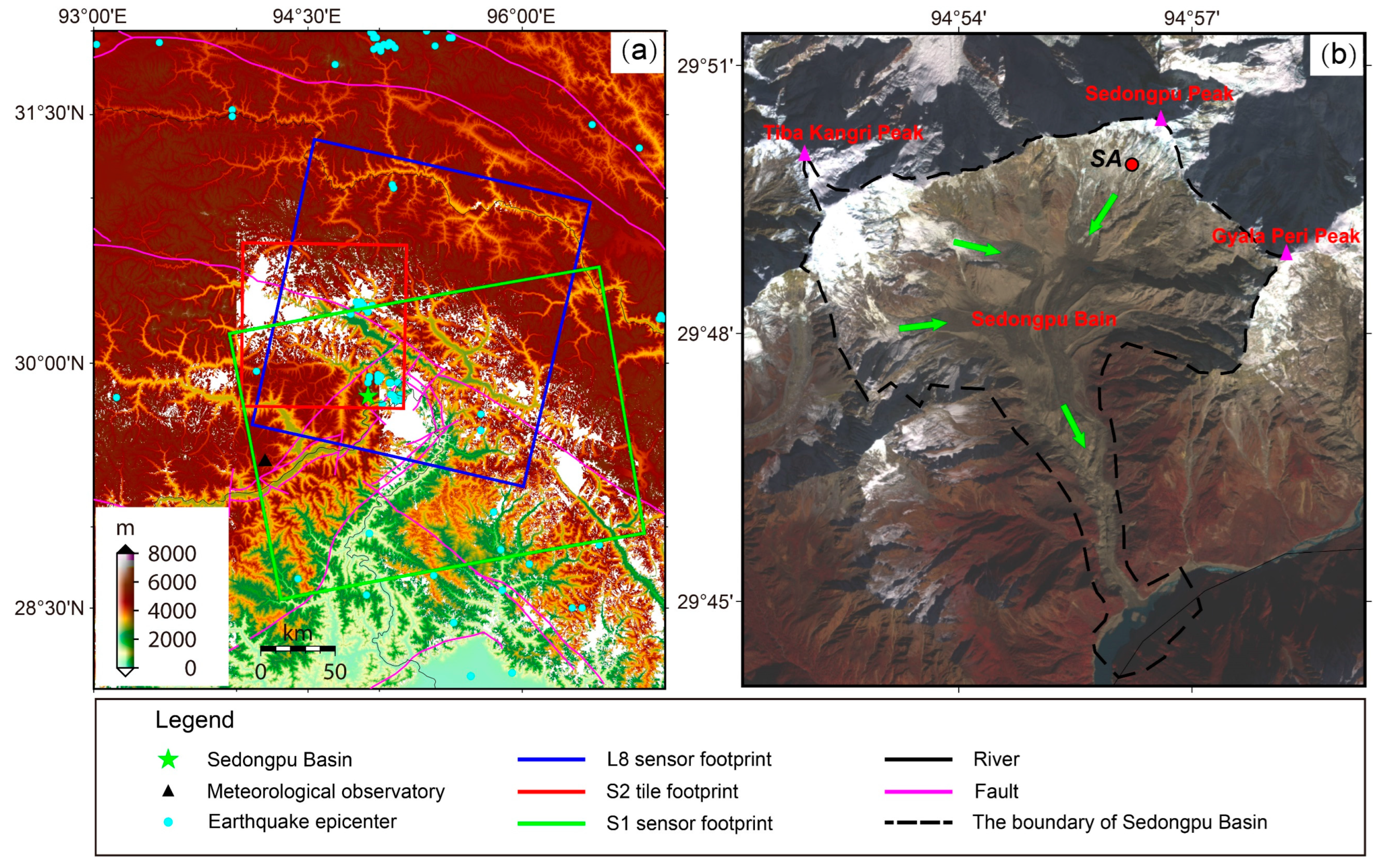
Funding

This research was funded by the open foundation of the State Key Laboratory of Geodesy and Earth’s Dynamics (Grant No. SKLGED2022-2-3), funded by Open Research Fund Program of LIESMARS (Grant No. 22R03), and the Shandong Provincial Natural Science Foundation, China (Grant No. ZR2021QD075).

Data Availability Statement

No applicable.

Acknowledgments

The COSI-Corr (Co-registration of Optically Sensed Images and Correlation) software developed by the California Institute of Technology (Caltech) was used to calculate the optical cross-correlation results. The GAMMA software was the platform for acquiring the SAR offset-tracking results. Some figures in this paper were plotted with the GMT (Generic Mapping Tools) software.

Conflicts of Interest

The authors declare no conflict of interest.

References

  1. Liu, S.; Yao, X.; Guo, W.; Xu, J.; Shangguan, D.; Wei, J.; Bao, W.; Wi, L. The contemporary glaciers in China based on the Second Chinese Glacier Inventory. Acta Geogr. Sin. 2015, 77, 3–16. [Google Scholar]
  2. Fu, X. Research on Detection of Glacier Changes in Western China by Remote Sensing. Ph.D. Thesis, University of Chinese Academy of Sciences, Beijing, China, 2019. (In Chinese). [Google Scholar]
  3. Wu, G.; Yao, T.; Wang, W.; Zhao, H.; Yang, W.; Zhang, G.; Li, S.; Yu, W.; Lei, Y.; Hu, W. Glacial Hazards on Tibetan Plateau and Surrounding Alpines. Bull. Chin. Acad. Sci. 2019, 34, 8. (In Chinese) [Google Scholar]
  4. Wu, L.; Li, J.; Miao, Z.; Wang, W.; Chen, B.; Li, Z.; Dai, W.; Xu, W. Pattern and directions of spaceborne- airborne-ground collaborated intelligent monitoring on the geo-hazards developing environment and disasters in glacial basin. Acta Geod. Cartogr. Sin. 2021, 50, 1109–1121. (In Chinese) [Google Scholar]
  5. Yao, T.; Li, Z.; Yang, W.; Guo, X.; Zhu, L.; Kang, S.; Wu, Y.; Yu, W. Glacial distribution and mass balance in the Yarlung Zangbo River and its influence on lakes. Chin. Sci. Bull. 2010, 55. (In Chinese) [Google Scholar] [CrossRef]
  6. Tong, L.; Tu, J.; Pei, L.; Zhaocheng, G.; Xiongwei, Z.; Jinghui, F.; Chang, Z.; Chunling, L.; Shashan, W.; Peng, H.E.; et al. Preliminary discussion of the frequently debris flow events in Sedongpu Basin at Gyalaperi peak, Yarlung Zangbo River. J. Eng. Geol. 2018, 26, 1552–1561. (In Chinese) [Google Scholar]
  7. Liu, C.; Lü, J.; Tong, L.; Chen, H.; Liu, Q.; Xiao, R.; Tu, J. Research on glacial/rock fall-landslide-debris flows in Sedongpu basin along Yarlung Zangbo River in Tibet. Geol. China 2019, 46, 219–234, (In Chinese with English abstract). [Google Scholar]
  8. Li, W.; Zhao, B.; Xu, Q.; Scaringi, G.; Lu, H.; Huang, R. More frequent glacier-rock avalanches in Sedongpu gully are blocking the Yarlung Zangbo River in eastern Tibet. Landslides 2022, 19, 589–601. [Google Scholar] [CrossRef]
  9. Kääb, A.; Jacquemart, M.; Gilbert, A.; Leinss, S.; Girod, L.; Huggel, C.; Falaschi, D.; Ugalde, F.; Petrakov, D.; Chernomorets, S.; et al. Sudden large-volume detachments of low-angle mountain glaciers—More frequent than thought? Cryosphere 2021, 15, 1751–1785. [Google Scholar] [CrossRef]
  10. Liu, Y.; Shi, Z. Study on the surface deformation of ice avalanche debris flow movement area in Sedongpu Basin of Yarlung Zangbo river based on time series InSAR. J. Yunan Norm. Univ. Nat. Sci. Ed. 2021, 41, 63–70. (In Chinese) [Google Scholar]
  11. Zhu, B.; Ren, Z.; Zhang, Q.; Li, Y.; Wang, X. Glacier deformation inversion before disaster using SABS-InSAR technology in Sedongpu basin along the Yarlung Zangbo River. Bull. Surv. Mapp. 2021, 11, 31–35. (In Chinese) [Google Scholar]
  12. Li, K.; Zhang, M.; Xing, A. Numerical runout modeling and dynamic analysis of the ice avalanche-debris flow in Sedongpu Basin along Yarlung Zangbo River in Tibet. Chin. J. Geol. Hazard Control 2021, 32, 18–27. (In Chinese) [Google Scholar]
  13. Zhao, C.; Yang, W.; Westoby, M.; An, B.; Wu, G.; Wang, W.; Wang, Z.; Wang, Y.; Dunning, S. Brief communication: An approximately 50 Mm3 ice-rock avalanche on 22 March 2021 in the Sedongpu valley, southeastern Tibetan Plateau. Cryosphere 2022, 16, 1333–1340. [Google Scholar] [CrossRef]
  14. Li, Z.; Sun, J.; Gao, M.; Fu, G.; An, Z.; Zhao, Y.; Fang, L.; Guo, X. Evaluation of horizontal ground motion waveforms at Sedongpu Glacier during the 2017 M6.9 Mainling earthquake based on the equivalent Green’s function. Eng. Geol. 2022, 306, 106743. [Google Scholar] [CrossRef]
  15. Ding, C.; Feng, G.; Liao, M.; Tao, P.; Zhang, L.; Xu, Q. Displacement history and potential triggering factors of Baige landslides, China revealed by optical imagery time series. Remote Sens. Environ. 2021, 254, 112253. [Google Scholar] [CrossRef]
  16. Li, M.; Zhang, L.; Ding, C.; Li, W.; Luo, H.; Liao, M.; Xu, Q. Retrieval of historical surface displacements of the Baige landslide from time-series SAR observations for retrospective analysis of the collapse event. Remote Sens. Environ. 2020, 240, 111695. [Google Scholar] [CrossRef]
  17. Dille, A.; Kervyn, F.; Handwerger, A.L.; d’Oreye, N.; Derauw, D.; Bibentyo, T.M.; Samsonov, S.; Malet, J.P.; Kervyn, M.; Dewitte, O. When image correlation is needed: Unravelling the complex dynamics of a slow-moving landslide in the tropics with dense radar and optical time series. Remote Sens. Environ. 2021, 258, 112402. [Google Scholar] [CrossRef]
  18. Lacroix, P.; Bièvre, G.; Pathier, E.; Kniess, U.; Jongmans, D. Use of Sentinel-2 images for the detection of precursory motions before landslide failures. Remote Sens. Environ. 2018, 215, 507–516. [Google Scholar] [CrossRef]
  19. Casagli, N.; Intrieri, E.; Tofani, V.; Gigli, G.; Raspini, F. Landslide detection, monitoring and prediction with remote-sensing techniques. Nat. Rev. Earth Environ. 2023, 4, 51–64. [Google Scholar] [CrossRef]
  20. Stumpf, A.S.; Michea, D.; Malet, J.P. Improved co-registration of Sentinel-2 and Landsat-8 imagery for earth surface motion measurements. Remote Sens. 2018, 10, 160. [Google Scholar] [CrossRef]
  21. Bontemps, N.; Lacroix, P.; Doin, M.P. Inversion of deformation fields time-series from optical images, and application to the long term kinematics of slow-moving landslides in Peru. Remote Sens. Environ. 2018, 210, 144–158. [Google Scholar] [CrossRef]
  22. Lacroix, P.; Araujo, G.; Hollingsworth, J.; Taipe, E. Self entrainment motion of a slow-moving landslide inferred from Landsat-8 time series. J. Geophys. Res. Earth Surf. 2019, 124, 1201–1216. [Google Scholar] [CrossRef]
  23. Li, Z.; Li, B.; Gao, Y.; Wang, M.; Zhao, C.; Liu, X. Remote sensing interpretation of development characteristics of high-position geological hazards in Sedongpu gully, downstream of Yarlung Zangbo River. Chin. J. Geol. Hazard Control. 2021, 32, 33–41. [Google Scholar] [CrossRef]
  24. Zhao, Y.; Wan, Z.; Tu, G.; Deng, H. Studying on Evolutionary Model and Susceptibility Mapping for Barrier Lake in Tibet of China. J. Hebei GEO Univ. 2020, 43, 55–64. (In Chinese) [Google Scholar]
  25. Zhang, T.; Gao, Y.; Li, B.; Yin, Y.; Liu, X.; Gao, H.; Yang, W. Characteristics of rock-ice avalanches and geohazard-chains in the Parlung Zangbo Basin, Tibet, China. Geomorphology 2023, 422, 108549. [Google Scholar] [CrossRef]
  26. Ding, C.; Zhang, L.; Liao, M.; Feng, G.; Dong, J.; Ao, M.; Yu, Y. Quantifying the spatio-temporal patterns of dune migration near Minqin Oasis in northwestern China with time series of Landsat-8 and Sentinel-2 observations. Remote Sens. Environ. 2020, 236, 111498. [Google Scholar] [CrossRef]
  27. Ayoub, F.; Leprince, S.; Avouac, J.P. COSI-CORR User’s Guide. Co-Registration of Optically Sensed Images and Correlation; Califonia Institute of Technology: Pasadena, CA, USA, 2015. [Google Scholar]
  28. Ding, C.; Feng, G.; Li, Z.; Shan, X.; Du, Y.; Wang, H. Spatio-temporal error sources analysis and accuracy improvement in Landsat 8 image ground displacement measurements. Remote Sens. 2016, 8, 937. [Google Scholar] [CrossRef]
  29. Ding, C.; Feng, G.; Liao, M.; Zhang, L. Change detection, risk assessment and mass balance of mobile dune fields near Dunhuang Oasis with optical imagery and global terrain datasets. Int. J. Digit. Earth 2020, 13, 1604–1623. [Google Scholar] [CrossRef]
  30. Zhou, Y.; Li, X.; Zheng, D.; Li, Z.; An, B.; Wang, Y.; Jiang, D.; Su, J.; Cao, B. The joint driving effects of climate and weather changes caused the Chamoli glacier-rock avalanche in the high altitudes of the India Himalaya. Sci. China Earth Sci. 2021, 64, 1909–1921. [Google Scholar] [CrossRef]
  31. Yang, C.; Wei, C.; Ding, H.; Wei, Y. Inversion of Glacier 3D Displacement from Sentinel-1 and Landsat 8 Images Based on Variance Component Estimation: A Case Study in Shishapangma Peak, Tibet, China. Remote Sens. 2023, 15, 4. [Google Scholar] [CrossRef]
  32. Aati, S.; Milliner, C.; Avouac, J.-P. A new approach for 2-D and 3-D precise measurements of ground deformation from optimized registration and correlation of optical images and ICA-based filtering of image geometry artifacts. Remote Sens. Environ. 2022, 277, 113038. [Google Scholar] [CrossRef]
  33. Zhou, Y.; Chen, G.; Qiao, X.; Lu, L. Mining High-Resolution KH-9 Panoramic Imagery to Determine Earthquake Deformation: Methods and Applications. IEEE Trans. Geosci. Remote Sens. 2022, 60, 1–12. [Google Scholar] [CrossRef]
  34. Hu, J. Theory and Method of Estimating Three-Dimensional Displacement with InSAR Based on the Modern Surveying Adjustment. Ph.D. Thesis, Central South University, Hunan, China, 2013. [Google Scholar]
  35. Shangguan, D.; Ding, Y.; Liu, S.; Xie, Z.; Pieczonka, T.; Xu, J.; Moldobekov, B. Quick release of internal water storage in a glacier leads to underestimation of the hazard potential of glacial lake outburst floods from Lake Merzbacher in Central Tian Shan Mountains. Geophys. Res. Lett. 2017, 44, 9786–9795. [Google Scholar] [CrossRef]
Figure 1. The physical geography of the Sedongpu Basin. (a) The regional topography and the image footprints of the study area, with the identification of the local geological faults and historical earthquakes. (b) The geographical environment of Sedongpu Basin was revealed with the false color composite map of Sentinel-2 (S2) NIR/Red/Blue bands acquired on 10 December 2017. The green arrows denote the potential flow direction of Sedongpu Glacier.
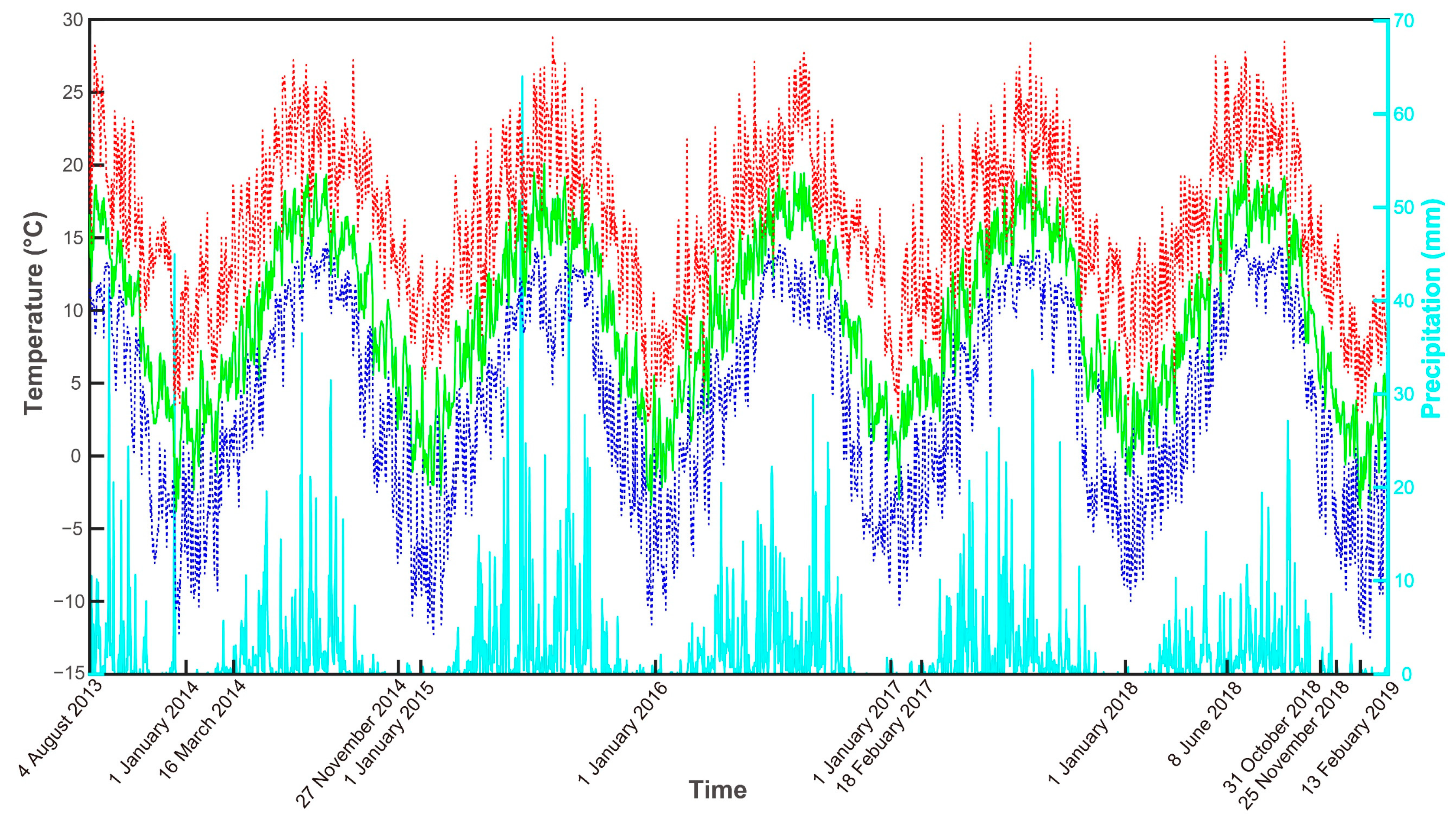
Remotesensing 15 02818 g001
Figure 2. The daily precipitation of Sedongpu Basin was downloaded from Giovanni, and the daily maximum (dotted red line), average (solid green line), and minimum (dotted blue line) air temperature was derived from a meteorological observation station located in Nyingchi County with an elevation of approximately 3000 m.
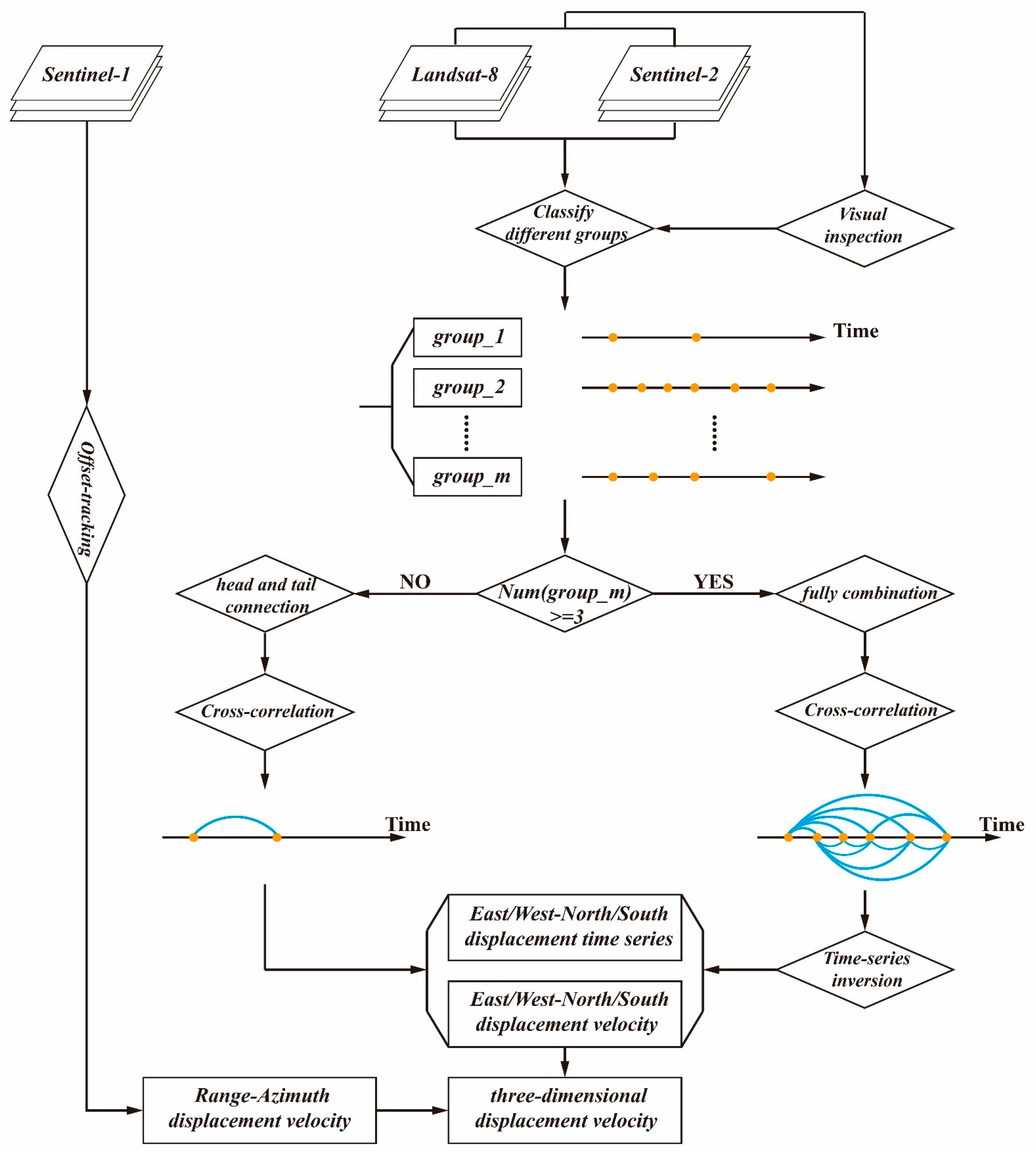
Remotesensing 15 02818 g002
Figure 3. Flowchart of the methodology proposed in this study.
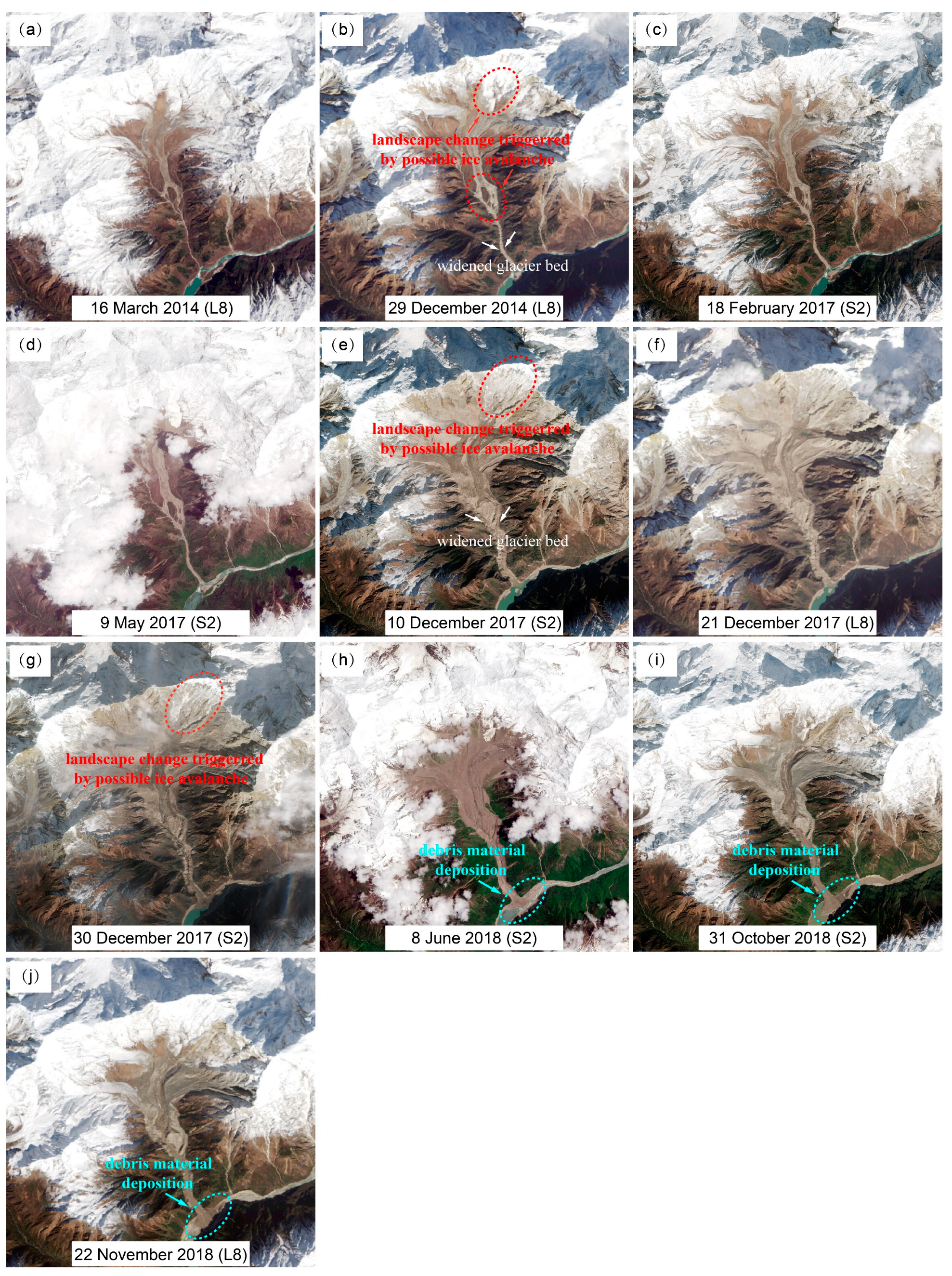
Remotesensing 15 02818 g003
Figure 4. The RGB real-colored combined time-series optical images of L8 and S2, in which the obvious ground geomorphic changes that may have been triggered by the ice-rock avalanches, debris flow events, and other glacial instability were emphatically highlighted. The subfigures (aj) denote the optical images acquired on 16 March 2014 (L8), 29 December 2014 (L8), 18 February 2017 (S2), 9 May 2017 (S2), 10 December 2017 (S2), 21 December 2017 (L8), 30 December 2017 (S2), 8 June 2018 (S2), 31 October 2018 (S2), 22 November 2018 (L8), respectively.
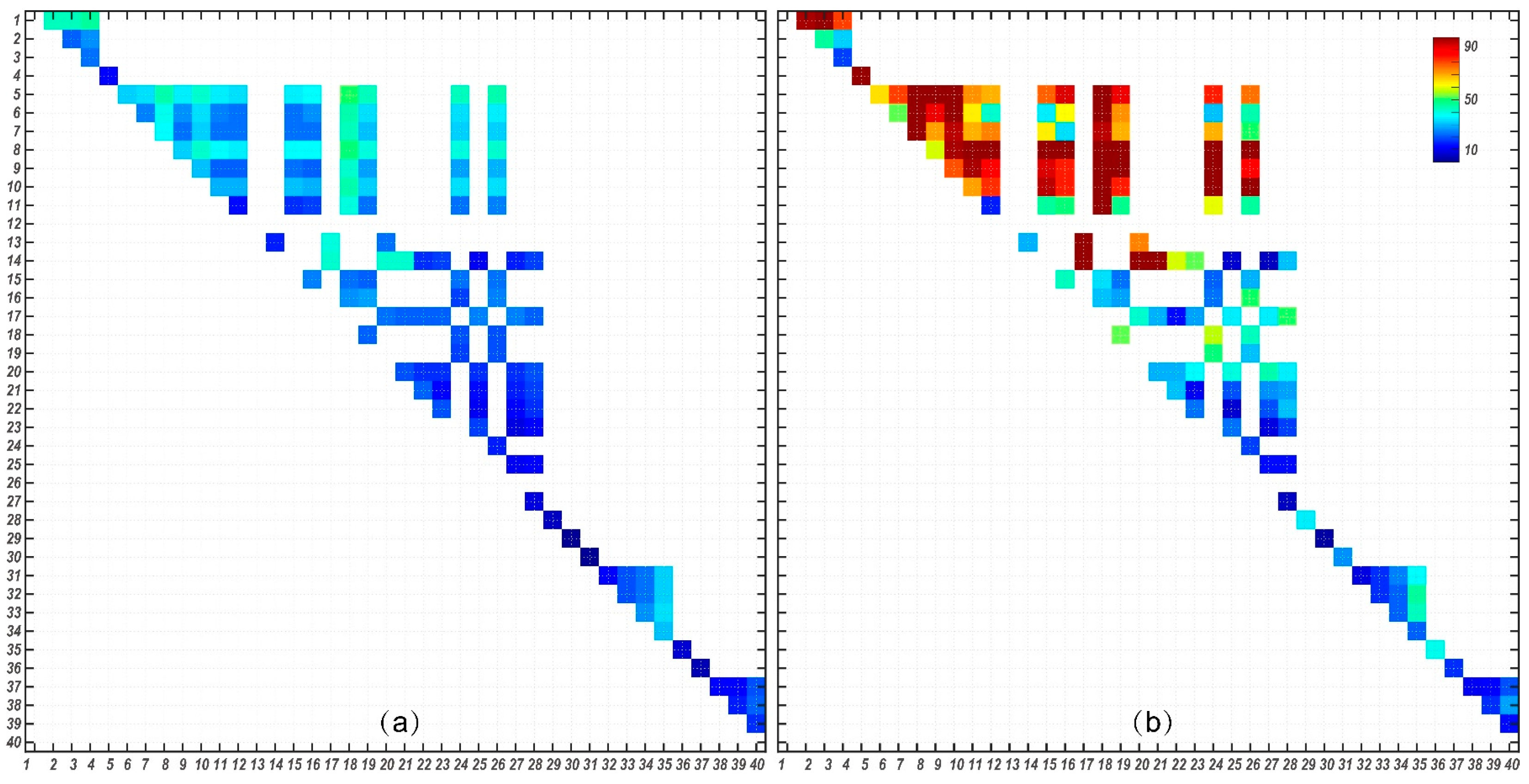
Remotesensing 15 02818 g004
Figure 5. (a) Standard deviations (STD) in the stable area of each correlation pair in different groups after the general noise reduction and time-series inversion. (b) Improvement of STD in the stable area of each correlation pair in comparison to the raw correlation pairs. The number labels of the horizontal axis and vertical axis denote the optical image acquisition sequence (see Table 2) in chronological order.
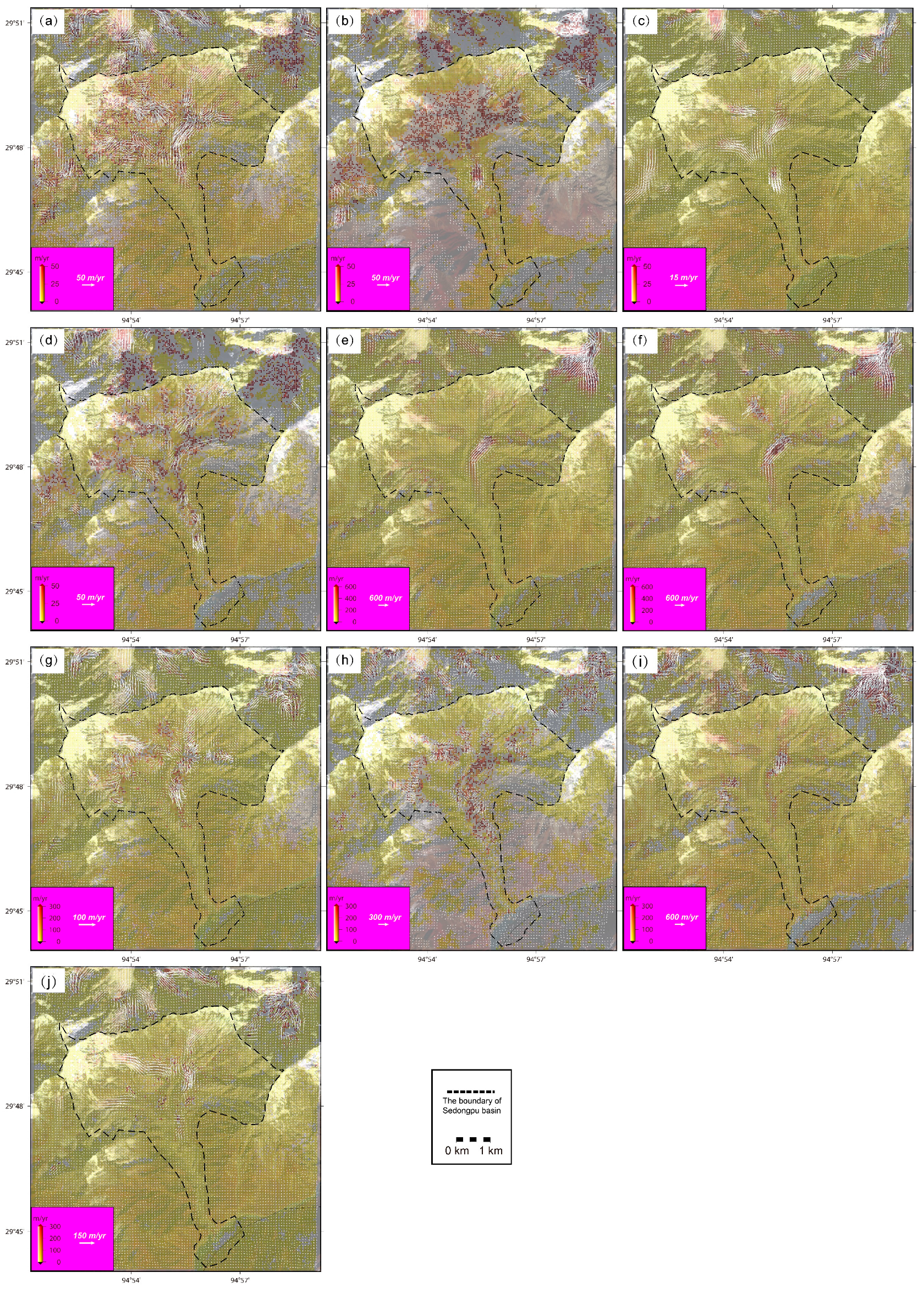
Remotesensing 15 02818 g005
Figure 6. The surface horizontal displacement velocity (m/yr) of active glaciers in Sedongpu Basin for the optical image groups with different time coverage. The subfigures (aj) denote the normalized horizontal displacement velocities of Group_1 (4 August 2013–16 March 2014), Group_1_2 (16 March 2014–27 November 2014), Group_2 (27 November 2014–18 February 2017), Group_2_3 (18 February 2017–10 December 2017), Group_3 (10 December 2017–20 December 2017), Group_3_4 (20 December 2017–30 December 2017), Group_4 (30 December 2017–8 June 2018), Group_4_5 (8 June 2018–31 October 2018), Group_5_6 (31 October 2018–25 November 2018), and Group_6 (25 November 2018–13 February 2019), respectively.
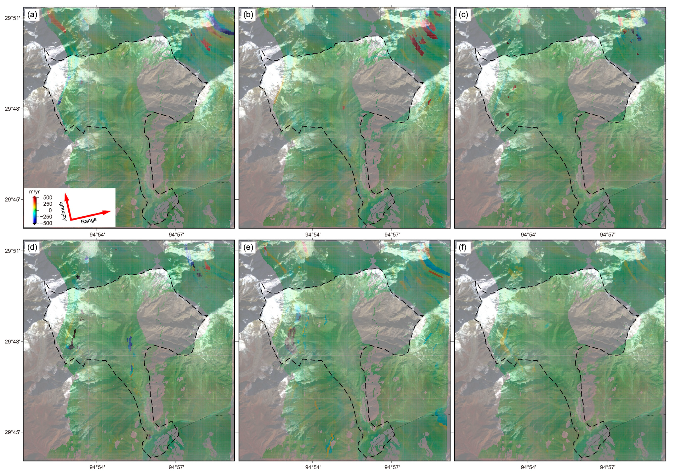
Remotesensing 15 02818 g006
Figure 7. The azimuth-oriented displacement velocity (cm/day) of active glaciers in Sedongpu Basin for the S1A SAR image groups with different time coverage, in which the subfigure (a) denotes the Group_3′ (5 December 2017–17 December 2017), the subfigure (b) denotes the Group_3′_4′ (17 December 2017–29 December 2017), the subfigure (c) denotes the Group_4′ (29 December 2017–3 June 2018), the subfigure (d) denotes the Group_4′_5′ (3 June 2018–25 October 2018), the subfigure (e) denotes the Group_5′_6′ (25 October 2018–30 November 2018), and the subfigure (f) denotes the Group_6′ (30 November 2018–10 February 2019), respectively. Measurements are positive toward the SAR sensor heading direction and negative toward the opposite direction.
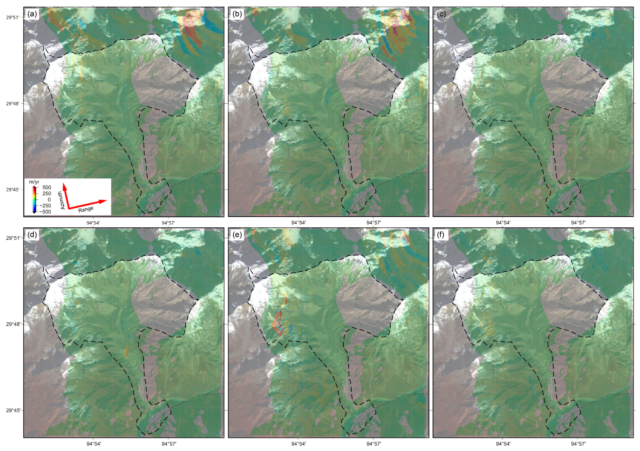
Remotesensing 15 02818 g007
Figure 8. The range-oriented displacement velocity (cm/day) of active glaciers in Sedongpu Basin for the S1A SAR image groups with different time coverage, in which the subfigure (a) denotes the Group_3′ (5 December 2017–17 December 2017), the subfigure (b) denotes the Group_3′_4′ (17 December 2017–29 December 2017), the subfigure (c) denotes the Group_4′ (29 December 2017–3 June 2018), the subfigure (d) denotes the Group_4′_5′ (3 June 2018–25 October 2018), the subfigure (e) denotes the Group_5′_6′ (25 October 2018–30 November 2018), and the subfigure (f) denotes the Group_6′ (30 November 2018–10 February 2019), respectively. Measurements are positive toward the radar pulse emission or range direction and negative toward the opposite direction.
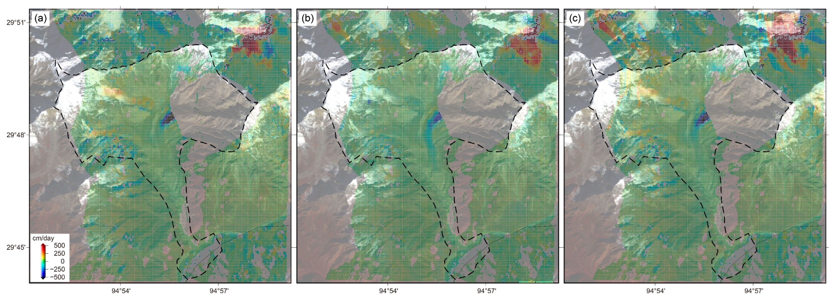
Remotesensing 15 02818 g008
Figure 9. The three-dimensional (3D) displacement velocity (cm/day) fields inverted from the optical Group_3 (10 December 2017–20 December 2017) and SAR Group_3′ (5 December 2017–17 December 2017) observations. (a) E/W oriented velocity fields; (b) N/S oriented velocity fields; and (c) vertical oriented velocity fields.
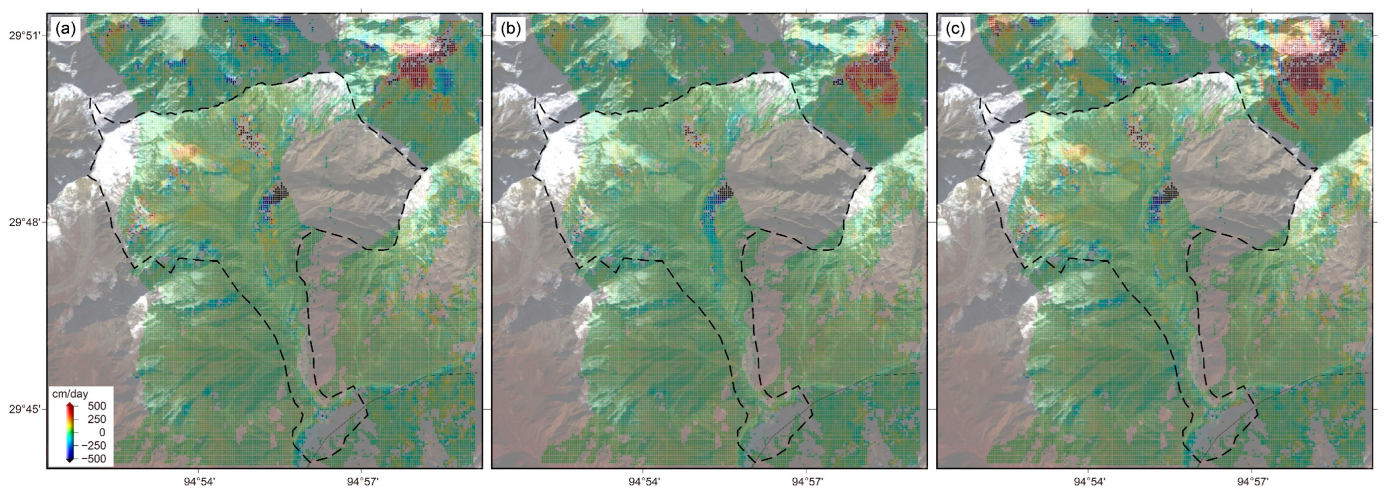
Remotesensing 15 02818 g009
Figure 10. The 3D displacement velocity (cm/day) fields inverted from the optical Group_3_4 (20 December 2017–30 December 2017) and SAR Group_3′_4′ (17 December 2017–29 December 2017) observations. (a) E/W oriented velocity fields; (b) N/S oriented velocity fields; and (c) vertically oriented velocity fields.
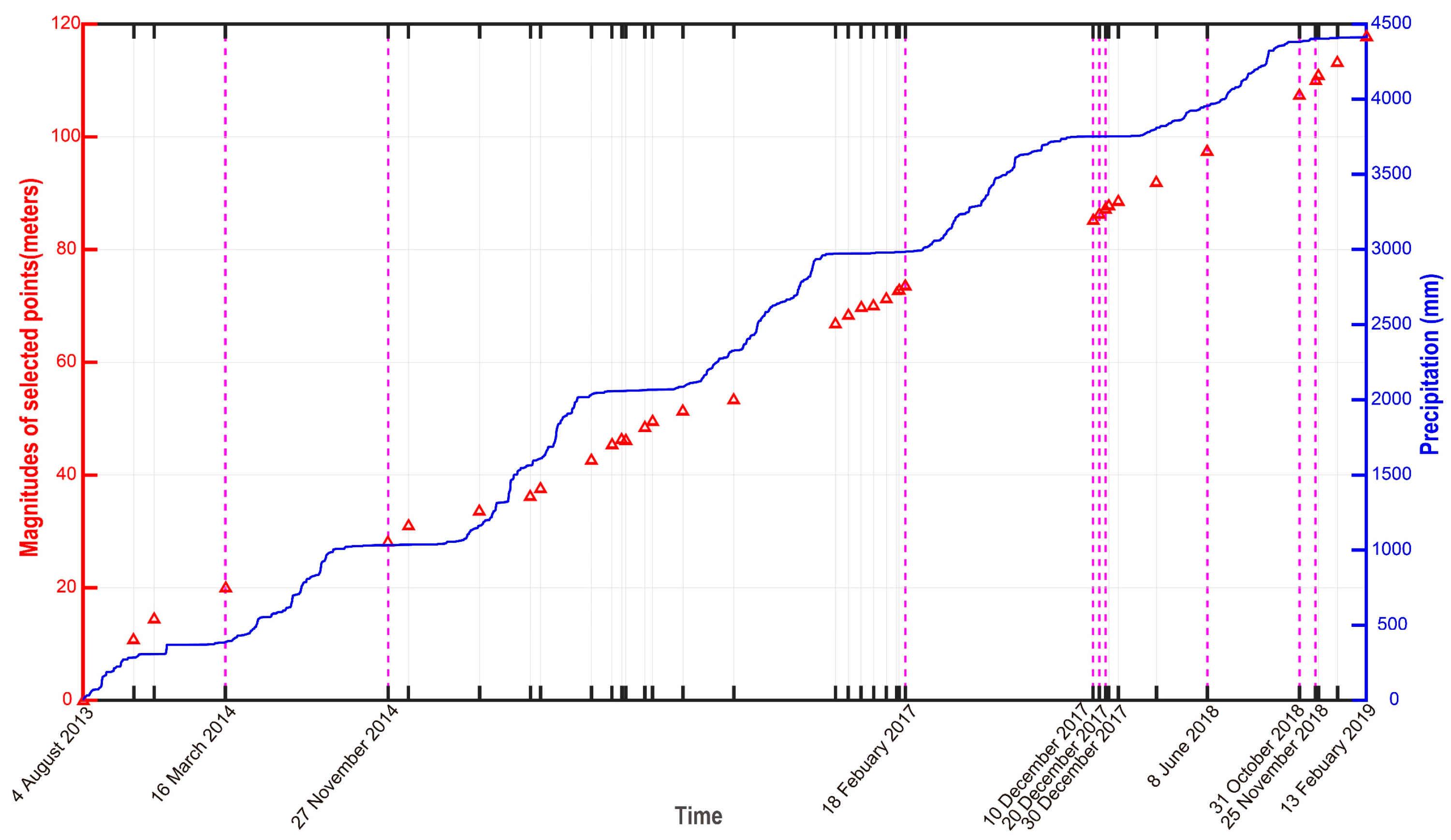
Remotesensing 15 02818 g010
Figure 11. The relationship between the displacement time series (m) of a point SA located in the source area of Sedongpu Glacier and the daily/cumulative precipitation (mm).
Remotesensing 15 02818 g011
Figure 12. The relationship between the displacement time series (m) of a point SA located in the source area of Sedongpu Glacier and the temperature variations of Nyingchi, a meteorological station located 40 km away from the Sedongpu Basin.
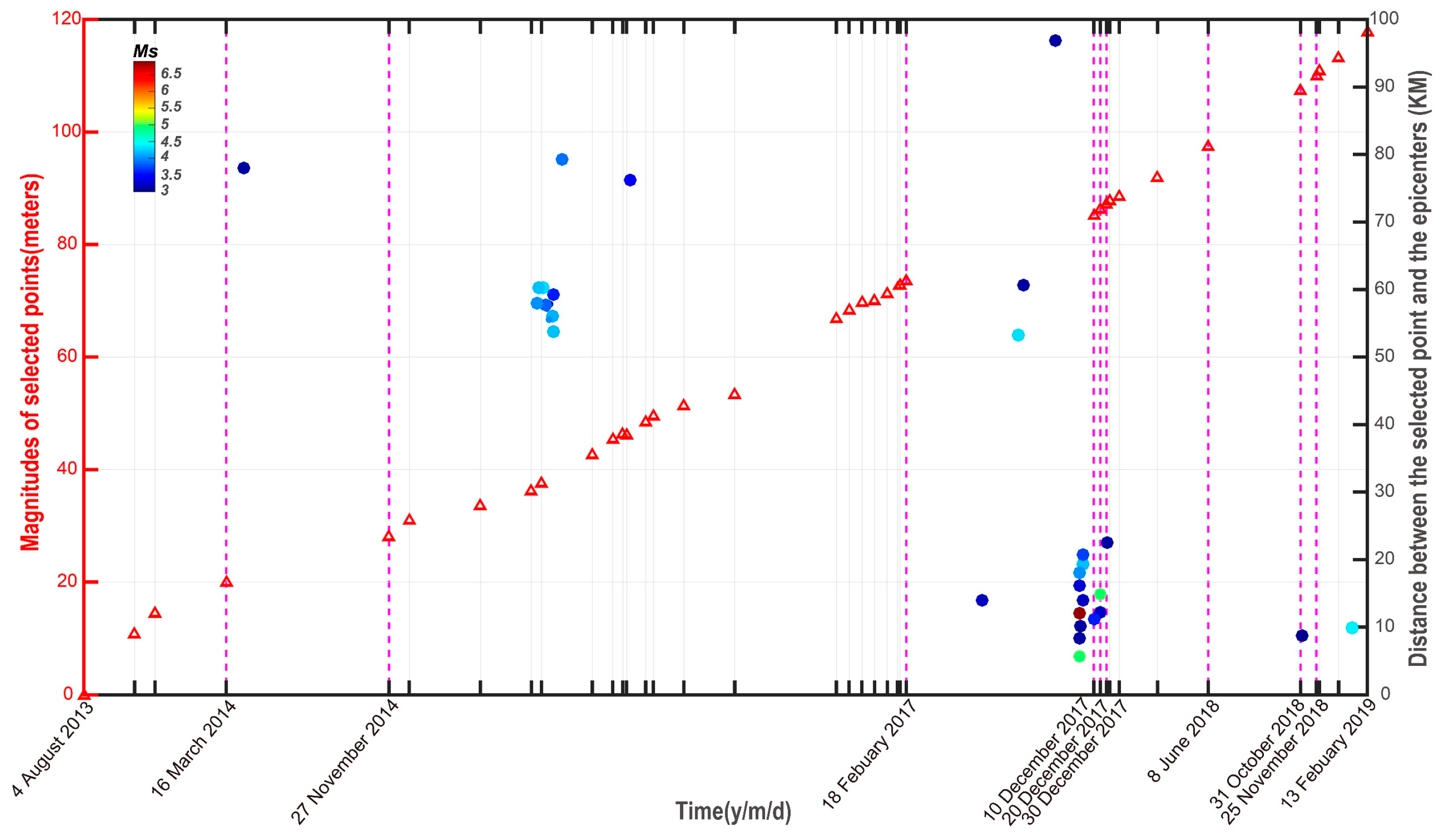
Remotesensing 15 02818 g012
Figure 13. The relationship between the displacement time series (m) of a point SA located in the source area of Sedongpu Glacier and the earthquake events with a circle distribution distance within 100 km.
Remotesensing 15 02818 g013
Table 1. The occurrence time of 8 historical debris flow and river blocking events.
SituationsImage Acquisition (Year/Month/Day)
Glacier debris flow events1969–1974, 2014, 22 October 2017, 28 October 2017, 21 December 2017, January 2018, 17 October 2018, 29 October 2018
Table 2. The parameter configuration for different sensors.
SensorsLandsat-8 (L8)Sentinel-2 (S2)Sentinel-1 (S1)
Image acquisition modesPush-broomPush-broomTOPS
LevelsL1CL1CL1
BandsNIRNIRVV
Incidence Angle//39.334°
Azimuth Angle//347.372°
Spatial resolution (m)15102.3 (range) × 14.1 (azimuth)
Image time coverageAugust 2013–November 2018December 2015–February 2019December 2017–February 2019
Number of images21217
Notes: The TOPS denotes the abbreviation of “Terrain Observation by Progressive Scans”.
Table 3. Image acquisition of L8, S2, and S1A sensors used in this study.
SensorsImage Acquisition (Year/Month/Day)
L84 August 2013, 23 October 2013, 24 November 2013, 16 March 2014, 27 November 2014, 29 December 2014, 20 April 2015, 9 July 2015, 25 July 2015, 13 October 2015, 14 November 2015, 30 November 2015, 17 January 2016, 5 March 2016, 24 May 2016, 31 October 2016, 19 January 2017, 4 February 2017, 21 December 2017, 22 January 2018, 22 November 2018
S26 December 2015, 5 January 2016, 5 May 2016, 31 October 2016, 20 November 2016, 10 December 2016, 30 December 2016, 19 January 2017, 8 February 2017, 18 February 2017, 10 December 2017, 20 December 2017, 30 December 2017, 4 January 2018, 19 January 2018, 20 March 2018, 31 October 2018, 25 November 2018, 30 November 2018, 30 December 2018, 13 February 2019
S1A5 December 2017, 17 December 2017, 29 December 2017, 3 June 2018, 25 October 2018, 30 November 2018, 10 February 2019
Table 4. The specific list of image acquisition and corresponding correlation pairs for different L8 and S2 image groups.
GroupsImage Acquisition (Year/Month/Day [Sensors#])Number of Correlation Pairs
14 August 2013 [L8]–23 October 2013 [L8]–24 November 2013 [L8]–16 March 2014 [L8]6 for L8
1→216 Marc 2014 [L8]–27 November 2014 [L8]1 for L8
227 November 2014 [L8]–29 December 2014 [L8]–20 April 2015 [L8]–9 July 2015 [L8]–25 July 2015 [L8]–13 October 2015 [L8]–14 November 2015 [L8]–30 November 2015 [L8]–6 December 2015 [S2]–5 January 2016 [S2]–17 January 2016 [L8]–5 March 2016 [L8]–5 March 2016 [S2]–24 May 2016 [L8]–31 October 2016 [L8]–31 October 2016 [S2]–20 November 2016 [S2]–10 December 2016 [S2]–30 December 2016 [S2]–19 January 2017 [L8]–19 January 2017 [S2]–4 February 2017 [L8]–8 February 2017 [S2]–18 February 2017 [S2]136
2→318 February 2017 [S2]–10 December 2017 [S2]1 for S2
310 December 2017 [S2]–20 December 2017 [S2]1 for S2
3→420 December 2017 [S2]–30 December 2017 [S2]1 for S2
430 December 2017 [S2]–4 January 2018 [S2]–19 January 2018 [S2]–20 March 2018 [S2]–8 June 2018 [S2]10 for S2
4→58 June 2018 [S2]–31 October 2018 [S2]1 for S2
531 October 2018 [S2]/
5→631 October 2018 [S2]–25 November 2018 [S2]1 for S2
635 October 2018 [S2]–30 November 2018 [S2]–30 December 2018 [S2]–13 February 2019 [S2]6 for S2
Table 5. Parameter configuration for optical image correlation processing.
Optical SensorsL8S2
Frequency correlatorSearch windowInitial size (pixels)64 × 6464 × 64
Final size (pixels)32 × 3232 × 32
Steps (pixels)4 × 46 × 6
Robust iterations22
Frequency mask0.90.9
Table 6. Different image groups of the S1A sensor were used in this study.
GroupsImage Acquisition (Year/Month/Day [Ascending])
3′5 December 2017–17 December 2017
3′→4′17 December 2017–29 December 2017
4′29 December 2017–3 June 2018
4′→5′3 June 2018–25 October 2018
5′25 October 2018
5′→6′25 October 2018–30 November 2018
6′30 November 2018–10 February 2019
Table 7. Parameters configuration used for S1A offset-tracking processing.
SensorsS1A
Range Correlation Window Size (Pixels)128
Azimuth Correlation Window Size (Pixels)128
Range Search Steps (Pixels)5
Azimuth Search Steps (Pixels)1
Mask Threshold0.01
Disclaimer/Publisher’s Note: The statements, opinions and data contained in all publications are solely those of the individual author(s) and contributor(s) and not of MDPI and/or the editor(s). MDPI and/or the editor(s) disclaim responsibility for any injury to people or property resulting from any ideas, methods, instructions or products referred to in the content.

