Article

An Automatic Method for Rice Mapping Based on Phenological Features with Sentinel-1 Time-Series Images

1
School of Computer and Information Engineering, Henan University, Kaifeng 475004, China
2
Henan Province Engineering Research Center of Spatial Information Processing, Kaifeng 475004, China
3
Henan Key Laboratory of Big Data Analysis and Processing, Kaifeng 475004, China
4
The Second Surveying and Mapping Institute of Hunan Province, Changsha 430103, China
5
Key Laboratory of Natural Resources Monitoring and Supervision in Southern Hilly Region, Ministry of Natural Resources, Changsha 430103, China
*
Author to whom correspondence should be addressed.
Remote Sens. 2023, 15(11), 2785; https://doi.org/10.3390/rs15112785
Submission received: 20 April 2023 / Revised: 19 May 2023 / Accepted: 22 May 2023 / Published: 26 May 2023
(This article belongs to the Section Biogeosciences Remote Sensing)

Abstract

:
Rice is one of the most important staple foods in the world, feeding more than 50% of the global population. However, rice is also a significant emitter of greenhouse gases and plays a role in global climate change. As a result, quickly and accurately obtaining the rice mapping is crucial for ensuring global food security and mitigating global warming. In this study, we proposed an automated rice mapping method called automated rice mapping using V-shaped phenological features of rice (Auto-RMVPF) based on the time-series Sentinel-1A images, which are composed of four main steps. First, the dynamic threshold method automatically extracts abundant rice samples by flooding signals. Second, the second-order difference method automatically extracts the phenological period of rice based on the scattering feature of rice samples. Then, the key “V” feature of the VH backscatter time series, which rises before and after rice transplanting due to flooding, is used for rice mapping. Finally, the farmland mask is extracted to avoid interference from non-farmland features on the rice map, and the median filter is applied to remove noise from the rice map and obtain the final spatial distribution of rice. The results show that the Auto-RMVPF method not only can automatically obtain abundant rice samples but also can extract the accurate phenological period of rice. At the same time, the accuracy of rice mapping is also satisfactory, with an overall accuracy is more than 95% and an F 1 score of over 0.91. The overall accuracy of the Auto-RMVPF method is improved by 2.8–12.2% compared with support vector machine (SVM) with an overall accuracy of 89.9% (25 training samples) and 92.2% (124 training samples), random forest (RF) with an overall accuracy of 82.8% (25 training samples) and 88.3% (124 training samples), and automated rice mapping using synthetic aperture radar flooding signals (ARM-SARFS) with an overall accuracy of 89.9%. Altogether, these experimental results suggest that the Auto-RMVPF method has broad prospects for automatic rice mapping, especially for mountainous regions where ground samples are often not easily accessible.

Graphical Abstract

1. Introduction

Rice is one of the most important crops and is widely planted in Asia, Africa, and Latin America [1]. As the staple food for half of the world’s population, it accounts for 12% of the global grain planting area [2]. However, rice has also become a significant emitter of greenhouse gases by emitting methane [3]. As a semi-aquatic crop with hygroscopic characteristics, rice also consumes a large amount of water resources every year [4]. Therefore, timely and accurate rice mapping is not only crucial for maintaining social stability and food security but also provides key guidance for global climate research and water resources management.
Currently, there are two main methods for obtaining the rice-planting area: one is through traditional human statistics, and the other is through remote-sensing monitoring. Traditional human statistics rely on field surveys and level-by-level summaries to obtain data. This process is not only time-consuming and labor-intensive but also subject to subjective factors. Data updating is slow, which can greatly limit its practical application [5,6]. Furthermore, in most cases, the data obtained through traditional survey methods can only describe the rice-planting area through tabular digits and cannot provide an intuitive spatial distribution map of rice. Compared with traditional methods, remote-sensing monitoring can provide real-time and accurate information on the growth and spatial distribution of rice. It also has the advantages of broader scope, higher efficiency, and lower cost [7,8,9]. With the rapid development of remote-sensing technology in recent decades, it has become the most common means of agricultural monitoring [10,11,12], such as estimating the phenological periods, yield, and height of rice [13,14,15,16,17,18,19].
Two kinds of remote-sensing data are widely used for rice mapping: optical data and synthetic aperture radar (SAR) data. Optical remote-sensing images have a suitable spatial resolution, and many previous studies have demonstrated their superiority in rice classification [20,21,22,23]. For example, rice mapping can be carried out by extracting the vegetation index (such as normalized difference vegetation index (NDVI) [24] and the enhanced vegetation index (EVI) [25]), as well as the water-related index (such as normalized difference water index (NDWI) [26], land surface water index (LSWI) [27]) during key periods of rice growth [28]. However, optical remote-sensing satellites are vulnerable to clouds, fog, light intensity, and poor weather. As a result, it is difficult to provide sufficient time-series data to continuously monitor the dynamic changes of rice in areas with long-term cloudy and rainy weather [29], such as in southern China. Compared with optical remote sensing, the SAR signal has all-day and all-weather monitoring capability. It can penetrate clouds and is not easily affected by weather factors. In addition, the SAR signal is very sensitive to the geometric structure and dielectric properties of the surface, which has a suitable monitoring capability for rice. The geometric structure of rice changes greatly during its growth process, making it difficult to use the single-phase SAR image to capture all growth information. Sentinel-1A images have a high temporal and spatial resolution, so time-series Sentinel-1A images are used for rice mapping in this study.
In recent years, the research on rice mapping can be divided into two main methods, namely the machine learning (ML)-based and the phenology-based methods. Firstly, the polarization parameters of dual- or full-polarization SAR are used for rice mapping based on prior knowledge or biological characteristic by unsupervised classification (such as k-means, ISODATA, etc.) and supervised classification (such as SVM, CNN, etc.) [9,30,31,32,33,34,35,36,37,38]. Moreover, temporal backscatter signatures of rice can also be well used for the machine-learning method based on SAR time-series data, which can capture the signals of critical growth periods of rice for rice mapping in cloudy regions [15,28,39,40,41]. In brief, machine-learning models are driven by abundant samples for accurate rice mapping, which can extract informative features automatically based on polarization parameters or temporal backscatter signatures [28,42,43,44,45]. However, collecting abundant samples is difficult in mountainous regions or on a large scale. The lack of a large number of training samples may limit the application of these methods. Secondly, another popular method is based on phenology. The backscattering coefficient during the whole growth cycle of rice will fluctuate in a relatively large range due to flooding signals and the changes of its own morphology. Many researchers identify rice by constructing decision trees based on the dynamic range or variance of the radar backscattering coefficient during the growth period and the length of the growing season of rice [2,46,47,48,49]. However, since some land covers have a dynamic range of backscatter coefficients similar to rice (such as grassland), it may be impossible to completely distinguish rice from other land covers with only these characteristics [2]. However, the “V”-shaped feature with a large fluctuation, in which the backscattering coefficient rises and then declines before and after the transplanting period, is a prominent distinguishing feature from other land covers. Hence, the “V”-shaped feature is widely used for identifying rice through the decision trees [50,51].
In summary, there are some challenges in using SAR images for rice mapping. Firstly, abundant samples should be used for decision trees for pre-training to ensure the accuracy of rice mapping. Secondly, the time windows with phenological features are manually determined based on prior knowledge of rice phenology, which greatly increases the limitations of rice mapping without prior knowledge. Finally, some threshold values are sensitive for the identification of rice varieties with the variation of soil water content [14,52].
This study proposes an automatic rice-mapping method based on Sentinel-1A data, which provides a solution to the above challenges. The objectives of this study are: (1) abundant samples of rice are generated automatically by a dynamic threshold method, (2) the time window with phenological features (“V”-shaped feature) is extracted automatically by the second-order difference method based on the abundant samples, (3) a decision tree, threshold values of which are insensitive to the identification of rice varieties with the variation of soil water content, is constructed for rice mapping based on the “V”-shaped feature, (4) the result of rice mapping obtained by the automated rice mapping using the “V”-shaped phenological features of rice (Auto-RMVPF) method is compared with those obtained by random forest (RF), support vector machine (SVM), and automated rice mapping using synthetic aperture radar flooding signals (ARM-SARFS) methods.

2. Study Area and Data

2.1. Study Area

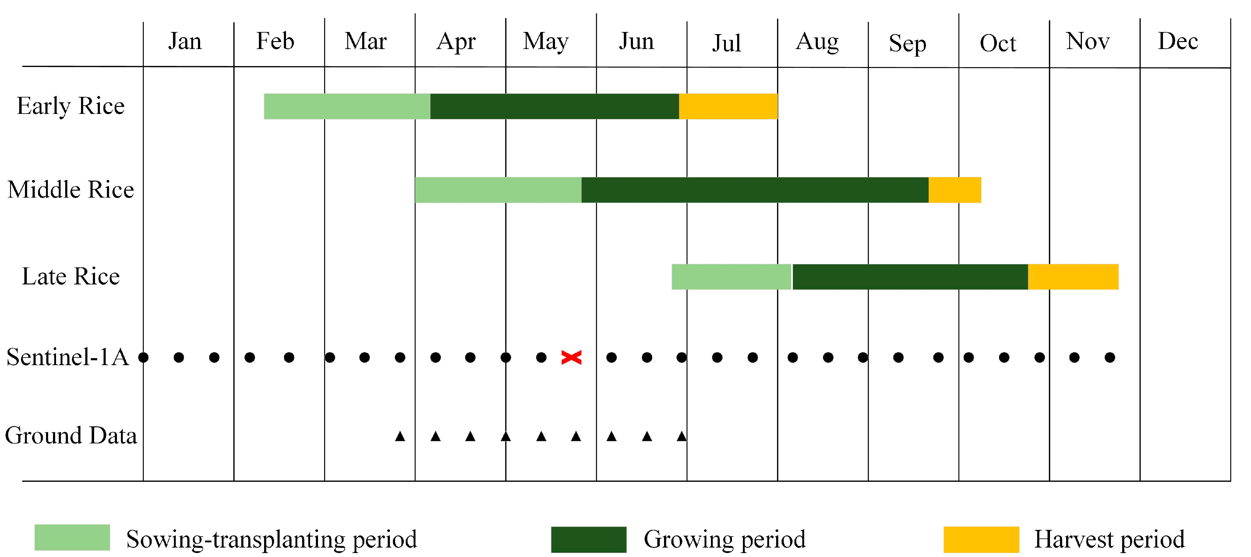
The study area with an area of 23 km × 32 km (21°55′N–22°12′N, 112°43′–112°56′) is located in Taishan Country, Guangdong Province, China, as shown in Figure 1. Taishan Country is an agricultural city, which is one of the national commodity grain bases. It is surrounded by mountains on three sides and faces the South China Sea in the south. The diverse landforms include hills, mountains, plains, coasts, and islands, with a relatively flat central terrain. Taishan Country has a subtropical marine monsoon climate, characterized by strong southerly winds in summer and strong northerly winds in winter. The weather is heavily influenced by the sea, resulting in long summers, mild winters, and plenty of rain, sunshine, and heat. The annual mean temperature, relative humidity, and precipitation (1981–2010) were 22.3 °C, 79, and 2002.6 mm, respectively. The climatic and geographical conditions are conducive to rice cultivation. In the study area, rice is typically grown twice a year and is known as early or late rice. Rice needs to be transplanted in this area. According to our ground data shown in Figure 2, the early rice is first sown and then flooded in mid-February, transplanted in late March or early April, and harvested in late June or early July.

2.2. Sentinel-1 SAR Data and Pre-Processing

In this study, we used time-series data of the Sentinel-1A for rice-extent mapping in the study area. The Sentinel-1A was launched by the European Space Agency (ESA) on 3 April 2014, with a C-band synthetic aperture radar (SAR) instrument operating at a central frequency of 5.405 GHz. The satellite orbits at a height of approximately 700 km and has an operational period of 12 days. The IW (interferometric wide swath) is the main acquisition mode on land, with a width of 250 km. We obtained 27 images with the Level 1 GRDH (ground-range detected high resolution) covering the study area on 27 dates in 2019 from the Copernicus Open Access Hub. All the images are in ascending pass. The GRDH product with IW (interferometric wide swath) mode has a spatial resolution of 10 m × 10 m and two polarization modes of VV and VH. The VH polarization is more sensitive to the growth state of rice than VV polarization, so we used VH polarization for rice mapping in this study [2].
We used the Sentinel Application Platform (SNAP) 6.0 software released by ESA to pre-process Sentinel-1A data. The pre-processing includes five steps: (1) correcting the orbit state of the Sentinel-1A images with the orbit file to obtain accurate satellite position and speed information, (2) performing radiometric calibration by converting the digital pixel value into backscattering coefficient in sigma naught ( σ 0 ), (3) applying speckle filtering with the refined Lee filtering (filter window is 7 pixels × 7 pixels) to reduce the impact of speckle noise and improve images quality, (4) performing range Doppler terrain correction with the shuttle radar topography mission (SRTM) digital elevation model, (5) converting the backscattering coefficient into dB units using Equation (1).
D N d B = 10 × l g σ 0
where D N d B is the output backscatter in dB units, and σ 0 is the backscattering coefficient.

2.3. Other Ancillary Data

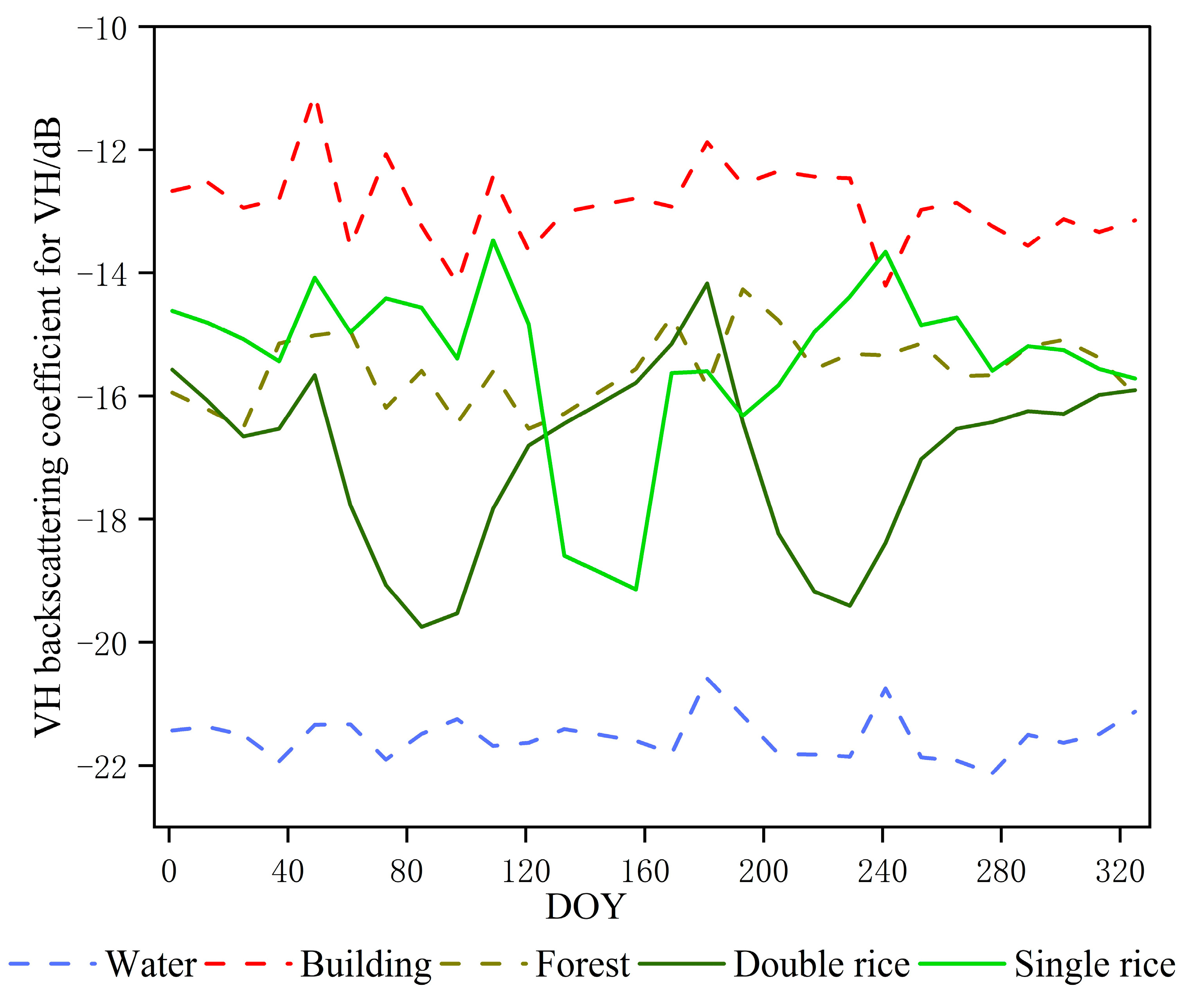
Other ancillary data used in this study include ground survey data, Google Earth high-resolution images, crop calendar data, and the public land-cover dataset. In order to comprehensively and accurately know the crop planting situation in the study area, we conducted a field survey in 2019. The location of the ground data was determined using a combination of paddy field surveys, GPS, and Google Earth. The specific campaign route and precise site locations are shown in Figure 1. The dates of data collection are consistent with the dates of Sentinel-1A acquisition, as shown in Figure 2. The ground survey data are used to select rice samples and land covers for VH backscatter coefficient analysis, as shown in Figure 3.
We used Google Earth high-resolution images in 2019 to supplement the samples through visual identification. We also obtained the crop calendar data in 2019 from the Ministry of Agriculture of the People’s Republic of China (http://www.moa.gov.cn/, 19 April 2023) to analyze phenological periods of rice in the study area and the 2019 Esri 10-Meter Land Cover data published by Esri to generate a farmland mask.
In this study, we conducted 9 detailed surveys on 20 paddy fields, as shown in Figure 2, with a single survey period interval of 12 days. The survey process lasted a total of 97 days and covered the growing period of early rice and the sowing–transplanting period of single rice. Through our ground survey, we were able to obtain detailed information on the transplanting and harvest dates of early rice, as well as the transplanting date of single-plant rice. This information was used to verify the accuracy of the extraction of phenological periods of rice. In addition, we used one region containing rice and non-rice fields, identified using Google Earth and field surveys, to verify the accuracy of rice mapping, as shown in Figure 1. In the verification region, we used a total of 75,144 pixels to calculate the confusion matrix for classification and test the classification accuracy of various methods, in which there are 22,223 rice pixels and 52,921 non-rice pixels. In the comparative experiment, we selected 25 training samples (13 rice and 12 non-rice) and 124 training samples (61 rice and 63 non-rice), respectively, to train the SVM and RF.

3. Methodology

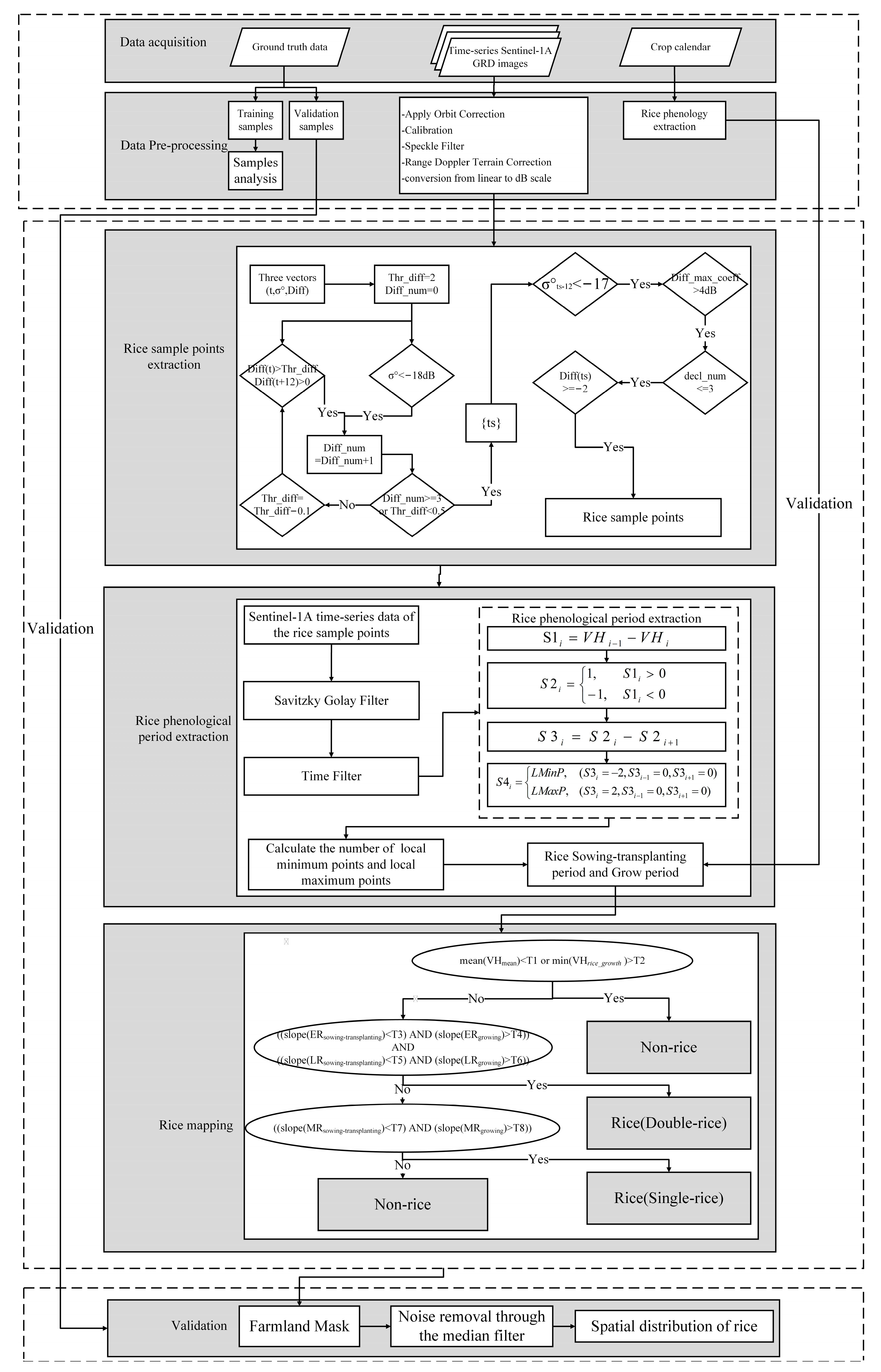
The framework of the Auto-RMVPF method used in this study consists of four main parts, as shown in Figure 4. Firstly, the dynamic threshold method automatically extracts abundant rice samples by flooding signals. Secondly, the second-order difference method extracts the growth period based on the analysis of the time-series VH backscattering coefficient of rice samples, which are extracted by the dynamic threshold method. Then, the growth periods of rice are input into the improved ARM-SARFS method for rice mapping. Finally, the post-processing with the farmland mask and median filter is carried out for the map of rice.

3.1. Extraction of the Rice Samples Based on the Dynamic Threshold Method

The dynamic threshold method is based on the time-series data of different lengths. The more Sentinel-1A images (i.e., the longer rice-planting time) obtained, the higher accuracy of extraction of rice samples. The vector σ 0 is extracted from a pixel of a set of time-series Sentinel-1A images. The vector σ 0 represents the sequence of VH backscattering coefficient values of this pixel, which is a collection of discrete observed values with an interval period of 12 days. Two other vectors of t and D i f f t are derived from the vector σ 0 . The t represents the acquisition date of the images (the day of year, DOY), which is an arithmetic sequence with a tolerance of 12 (the revisit period of Sentinel-1A satellite is 12 days). The D i f f t represents a set of differences between σ t + 12 0 and σ t 0 . The σ t 0 represents the VH backscattering coefficient values of rice in the image taken at date t [53]. The dynamic threshold method mainly includes the following four steps:
(1)
Extract the date on which the σ 0 is less than −18 dB;
(2)
Extract the date on which the D i f f t is less than T h r _ d i f f and D i f f t + 12 is greater than 0 dB. T h r _ d i f f is a dynamic threshold with a range of 0.5–2. The number of these dates is greater than 0 and less than 4. The method is shown in Figure 4;
(3)
Extract the dates t s that satisfy both step (1) and step (2);
(4)
Extract the date from t s , which satisfies the below conditions (a–d). When a date satisfies the below conditions, the pixel cycle is stopped, and the pixel is the rice sample point.
(a)
σ t s 12 0 < −18 dB. σ t s 12 0 is the backscattering coefficient at the date of DOY t s 12 ;
(b)
σ t x 0 ( t x t s + 12 , t c o e f f _ m a x ) is less than −13 dB and more than −21 dB. t c o e f f _ m a x is the date corresponding to σ m a x o . σ m a x o is the maximum backscattering coefficient from DOY p t to the latest date;
(c)
d e c l _ n u m s is not more than 3. d e c l _ n u m s is the number of D i f f t that is less than 0. In addition, t ranged from p t to t c o e f f _ m a x ;
(d)
D i f f t x 2 d B .

3.2. Extraction of the Rice Phenological Period Based on the Second-Order Difference Method

The phenological periods of rice can be automatically extracted by analyzing the time-series VH backscattering coefficient of the rice samples that are extracted by the dynamic threshold method (as shown in Figure 3).
According to the seasonal variation of rice, its entire growth period is generally divided into three important periods [54,55]: (1) the early irrigation period, which includes sowing, seedling, and transplanting; (2) the growth period, which includes panicle initiation, heading, and flowering; and (3) the harvesting and later periods. In this study, these three periods are defined as the sowing–transplanting period, the growing period, and the harvest period, respectively.
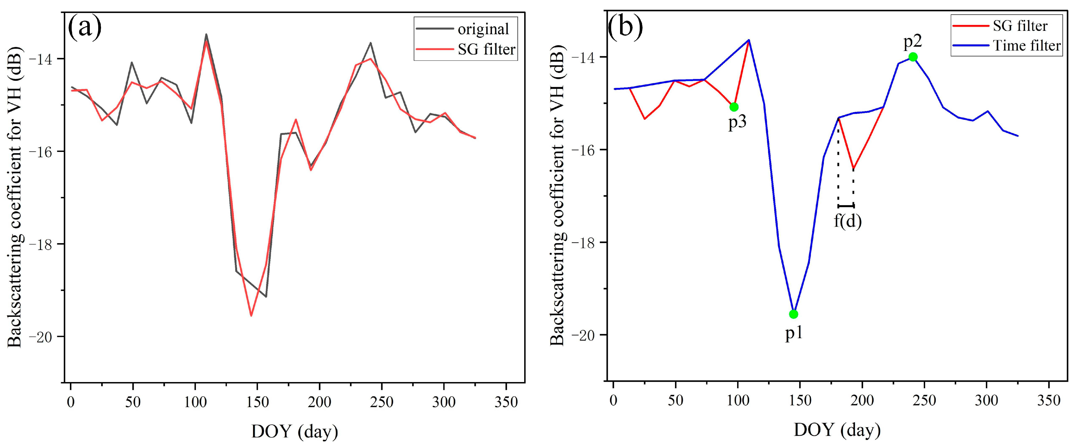
Based on the analysis of the VH backscattering features of rice in Figure 3, the local minimum point p 1 in the temporal scattering curve of VH is considered to be the transplanting date of rice (at this time, the VH backscattering coefficient value is small due to the large water-holding capacity of the paddy field), as shown in Figure 5b. The local maximum point p 2 is considered to be the maturity date of rice (at this time, the VH backscattering coefficient is higher because the paddy field is covered by vegetation information), as shown in Figure 5b.
Based on the time-series data, two filters are used to remove redundant local mutation information and extract local extreme value points. Firstly, the Savitzky–Golay (SG) filter is used to smooth the curve, as shown in Figure 5a. SG filtering can smooth the curve and ensure that the curve shape of the time-series data remains unchanged, which can accurately describe the changing trend of the time-series. Secondly, the time filter [28] is used on the time-series data that have been processed by the SG filter, as shown in Figure 5b. This makes the VH backscattering curve more consistent with the entire growth cycle of rice.
Ideally, each pair of p 1 and p 2 represents one rice-growth period. However, due to the influence of rainfall events or other environmental factors, there may be redundant local extreme points (e.g., p 3 in Figure 5b). This can bring errors to the extraction of the phenological period of rice. In general, environmental changes caused by rainfall events or other sudden factors can lead to a decrease in VH backscattering intensity (e.g., f d in Figure 5b). Therefore, a decline of fewer than 40 days in Sentinel-1A time-series data is filtered out by the time filter, such as f(d) in Figure 5b [28]. Finally, the second-order difference method can be used to extract the reliable local minimum and maximum points ( p 1 , p 2 ) as a growth period of rice.
The second-order difference method mainly includes the following four steps [56]:
(1)
Calculate the difference of VH backscattering coefficients at adjacent time points of vector σ 0 to obtain sequence S 1 .
S 1 i = V H i 1 V H i
(2)
The positive elements in sequence S 1 are marked as 1, and the negative elements in sequence S 1 are marked as −1, to obtain sequence S 2 . The results are shown in Figure 6b.
S 2 i = 1 ,   S 1 i > 0 1 ,   S 1 i < 0
(3)
Calculate the difference of adjacent elements in sequence S 2 to obtain sequence S 3 . The results are shown in Figure 6c.
S 3 i = S 2 i S 2 i + 1
(4)
The potential p 1 and p 2 are extracted from S 3 . One pair of p 1 and p 2 represents a growth period of rice (i.e., the growing period of rice), as shown in the red rectangle of Figure 6d. In sequence S 3 , the local maximum point p 2 appears where the element value is −2 and the value of its adjacent elements are both 0. Similarly, the local minima p 1 appear in sequence S 3 where the element value is 2 and the value of its adjacent elements are both 0.
Due to variations in geographical environments and rice varieties, the length of the rice-growing period differs. The early irrigation period of the sowing–transplanting period of rice typically takes about 45–75 days. However, in this study, the sowing–transplanting period of rice is defined as 60 days to accommodate rice planting in most areas. The sowing–transplanting period and growing period are used as input parameters for the decision tree in rice mapping.

3.3. Rice Mapping Based on the Improved ARM-SARFS Method

The VH backscattering curve exhibits distinct variations during different phenological periods of rice, as shown in Figure 3. This makes it possible to construct a decision tree model for rice mapping, which sets it apart from other land-cover types.
The ARM-SARFS method [2] builds a decision tree and sets relevant thresholds using prior knowledge. Then, using the annual average VH backscattering coefficient, the minimum VH backscattering coefficient during the entire growth period of rice (i.e., the sowing–transplanting period and growing period), the slope in different growth periods of rice, and the “V”-shaped feature of the flood signals before and after the rice transplanting period, it eliminates the non-crop areas and determines rice varieties [2]. The sensitivity test results [2] show that the ARM-SARFS method is insensitive to the threshold value and can obtain high classification accuracy within the range of −0.025 to 0. Even without training samples, satisfactory mapping accuracy can still be obtained in three research areas with different rice-planting types (1. southwestern part of Jianghan Plain, Hubei Province, with single and double rice, 2. Liaoning Province with single rice, 3. Guangdong Province with double rice), which demonstrates the robustness of the method.
However, there is still room for improvement in the ARM-SARFS method. Currently, it is only applicable to certain areas where phenological information on rice is available. The time window is determined by the rice phenological period and is manually set according to crop calendar data. As a result, the ARM-SARFS method cannot be applied in areas where crop calendar data are not available.
The improved ARM-SARFS method mainly includes the following three steps:
(1)
A threshold is used to eliminate non-cropland cover types. The average VH backscattering value for the whole year can be used to remove the water bodies, as their VH backscattering coefficient values are consistently low. Urban areas, artificial structures, and natural vegetation have high VH backscattering coefficient values, which are removed using the minimum value of VH backscattering during the entire growth period of rice. The non-cropland cover types are screened out using Formula (5):
m e a n V H y e a r < T 1   O R   m i n V H r i c e a l l _ g r o w t h > T 2
The V H y e a r represents the VH backscattering coefficient value during the whole year, and the V H r i c e a l l _ g r o w t h represents the VH backscattering coefficient value during the entire growth period of rice (i.e., the sowing–transplanting period and growing period). T 1 and T 2 are empirically set to −20 dB and −17 dB, respectively.
(2)
The slopes are used to identify double rice. If a pixel can be identified as the “V”-shaped feature of double rice, it is labeled as rice (double rice). The formula is as follows:
s l o p e E R s o w i n g t r a n s p l a n t i n g < T 3   AND   s l o p e E R g r o w i n g > T 4   AND s l o p e L R s o w i n g t r a n s p l a n t i n g < T 5   AND   s l o p e L R g r o w i n g > T 6
E R represents early rice, and L R represents late rice. T 3 and T 5 represent the thresholds for the VH backscatter slopes during the sowing–transplanting periods of early and late rice. Theoretically, T 3 and T 5 are equal to or less than 0. In this study, they are all set to 0. T 4 and T 6 represent the thresholds for the VH backscatter slopes during the growing periods of early and late rice, and they are empirically set to 0. The date (DOY) is taken as the independent variable, and the corresponding VH backscattering coefficient is taken as the predictor variable. The slopes are calculated using simple linear regression within the time window. The rice phenological period for calculating slopes is extracted using the second-order difference method presented in Section 3.2.
(3)
The slopes are used to identify single rice. If a pixel can identify the “V”-shaped feature of single rice, the pixel is labeled as rice (single rice). The formula is as follows:
s l o p e S R s o w i n g t r a n s p l a n t i n g < T 7   AND   s l o p e S R g r o w i n g > T 8
The S R represents the single rice. T 7 and T 8 , respectively, represent the thresholds for the VH backscatter slopes during the sowing–transplanting period and growing period of single rice. Theoretically, T 7 is equal to or less than 0 and T 8 is empirically set to 0. In this study, based on the analysis of the VH backscattering slopes for different phenological periods of individual rice samples in the study area, T7 is set to −0.009 and T8 is set to 0.02. The rice phenological period for calculating slopes is extracted by the second-order difference method presented in Section 3.2.

3.4. Noise Removal Based on Farmland Mask and Median Filter

The Esri 10-Meter Land Cover data (https://www.arcgis.com/apps/instant/media/index.html?appid=fc92d38533d440078f17678ebc20e8e2, accessed on 19 April 2023) published by Esri are a global land-cover dataset created using deep-learning methods based on Sentinel-2 images. The land covers in the dataset are classified into ten types (1. water, 2. trees, 3. grass, 4. flooded vegetation, 5. crops, 6. scrub/shrub, 7. built area, 8. bare ground, 9. snow/ice, 10. clouds). The crops, which are extracted from the dataset, are regarded as the input data of the median filter.
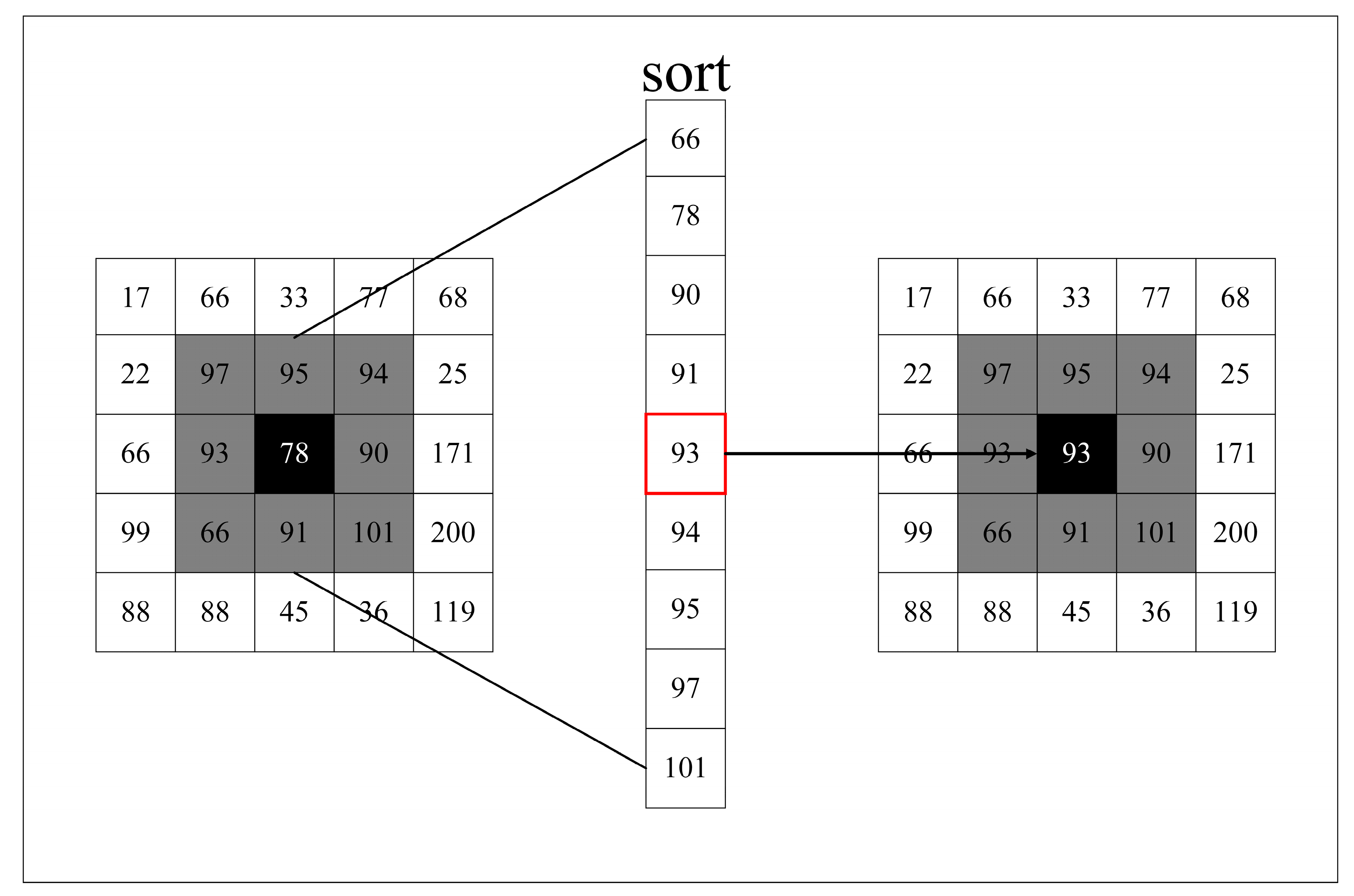
The median filter is a commonly used nonlinear filter. Its basic principle is as below: (1) select the pixel values of the current pixel and its adjacent pixel (an odd number of pixels), (2) sort these pixel values, and (3) take the middle-position pixel value as the value of the current pixel, as shown in Figure 7. The median filter is effective at eliminating isolated noise points because its primary function is to make the value of a pixel close to the values of its surrounding pixels. Additionally, the median filter can effectively preserve the boundary information of the paddy field while eliminating noise without causing significant blurring to the image.
The effectiveness of the median filter is greatly influenced by the size of the filtering window. There is a trade-off between noise elimination and detail preservation. If the filtering window is small, some details in the image can be well preserved, but some noise may remain in the image. On the other hand, a larger window size has better noise-filtering capabilities, but it may cause blurring in the image. Additionally, if the number of noise points in the filtering window is greater than the number of non-noise pixels in the whole window, the median filter may not effectively filter out the noise. In this study, based on the analysis presented in Section 5.3, the window size of the median filter was chosen to be 5.

4. Results

4.1. Rice Sample Extraction

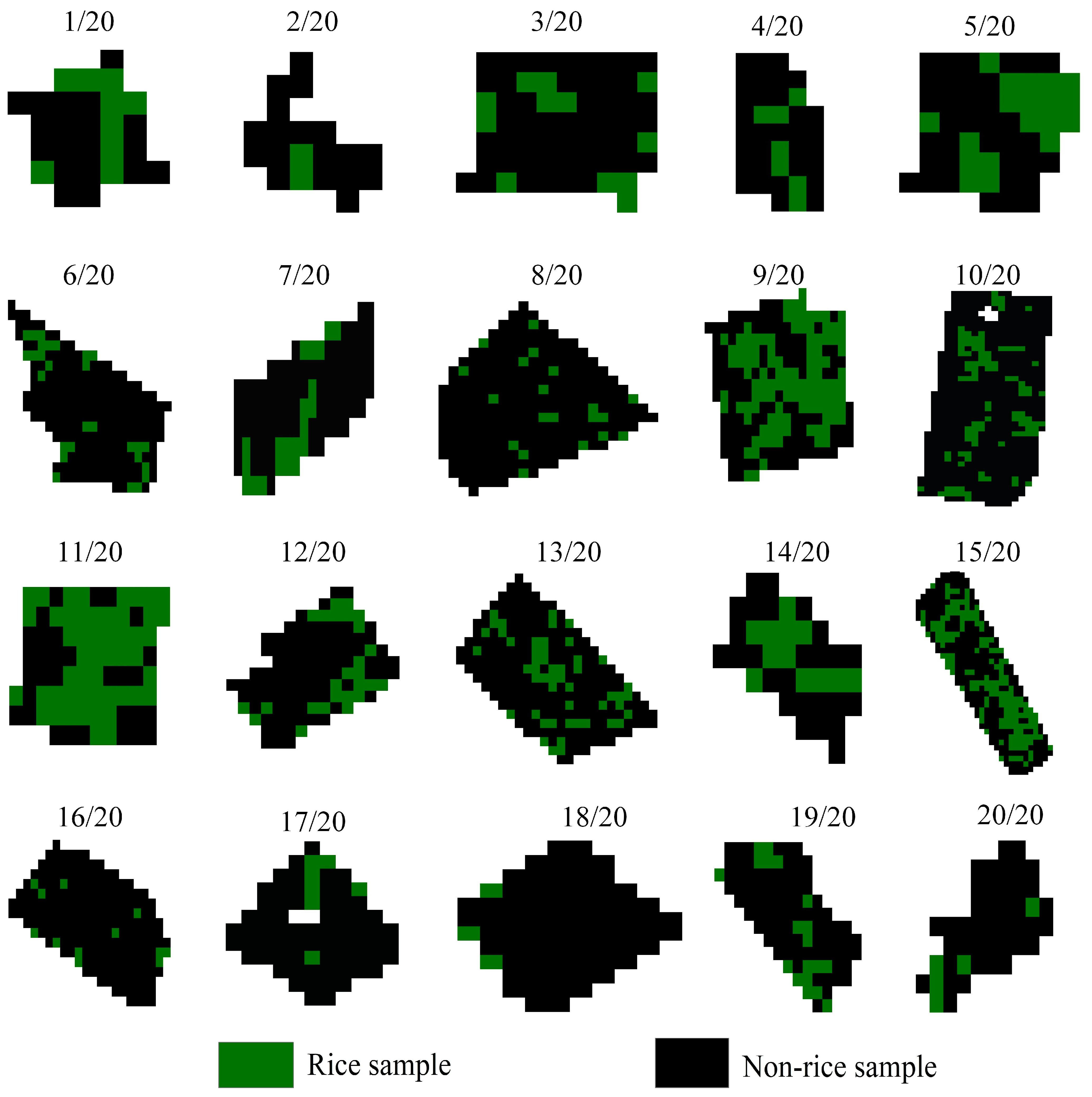
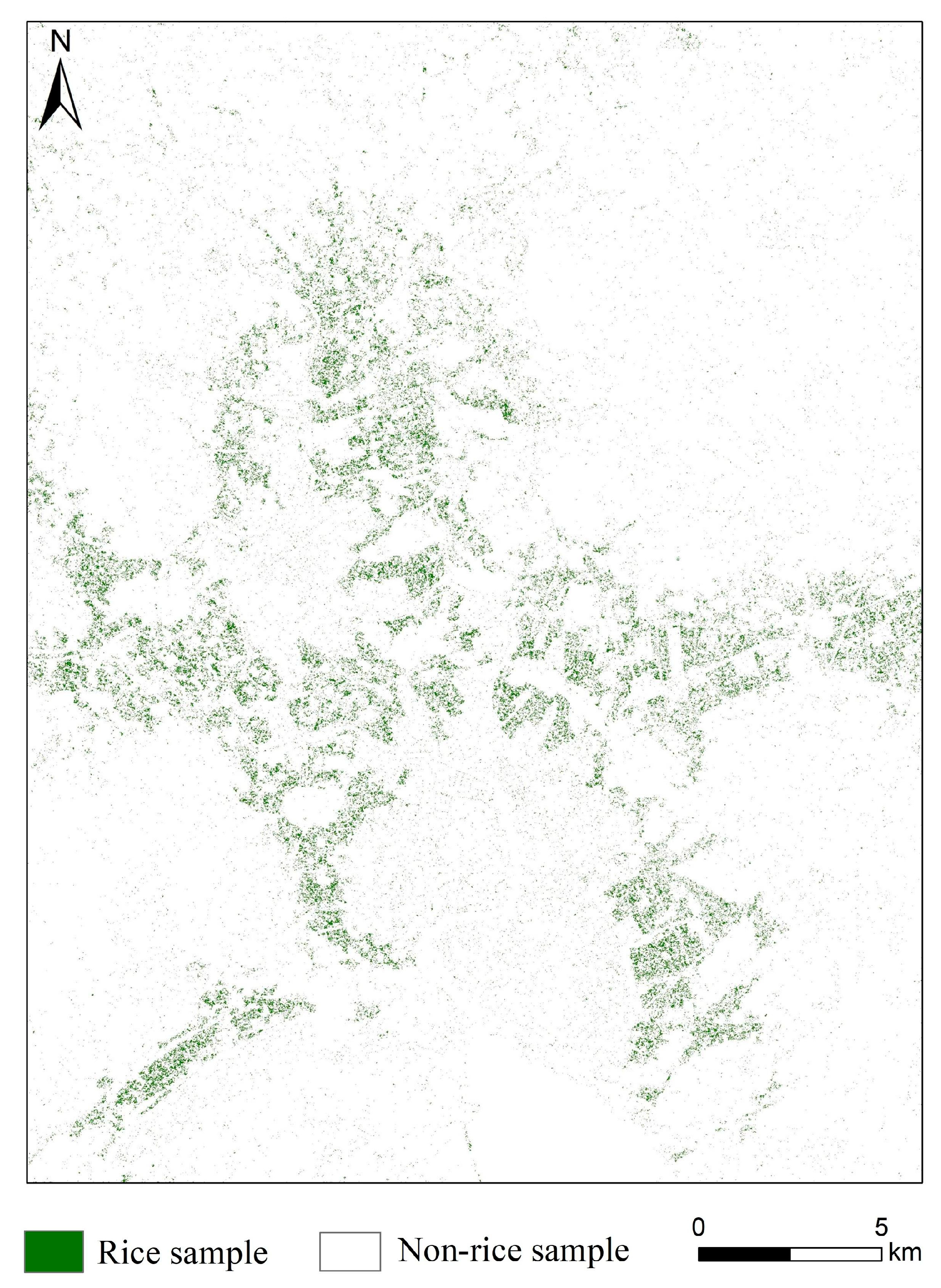
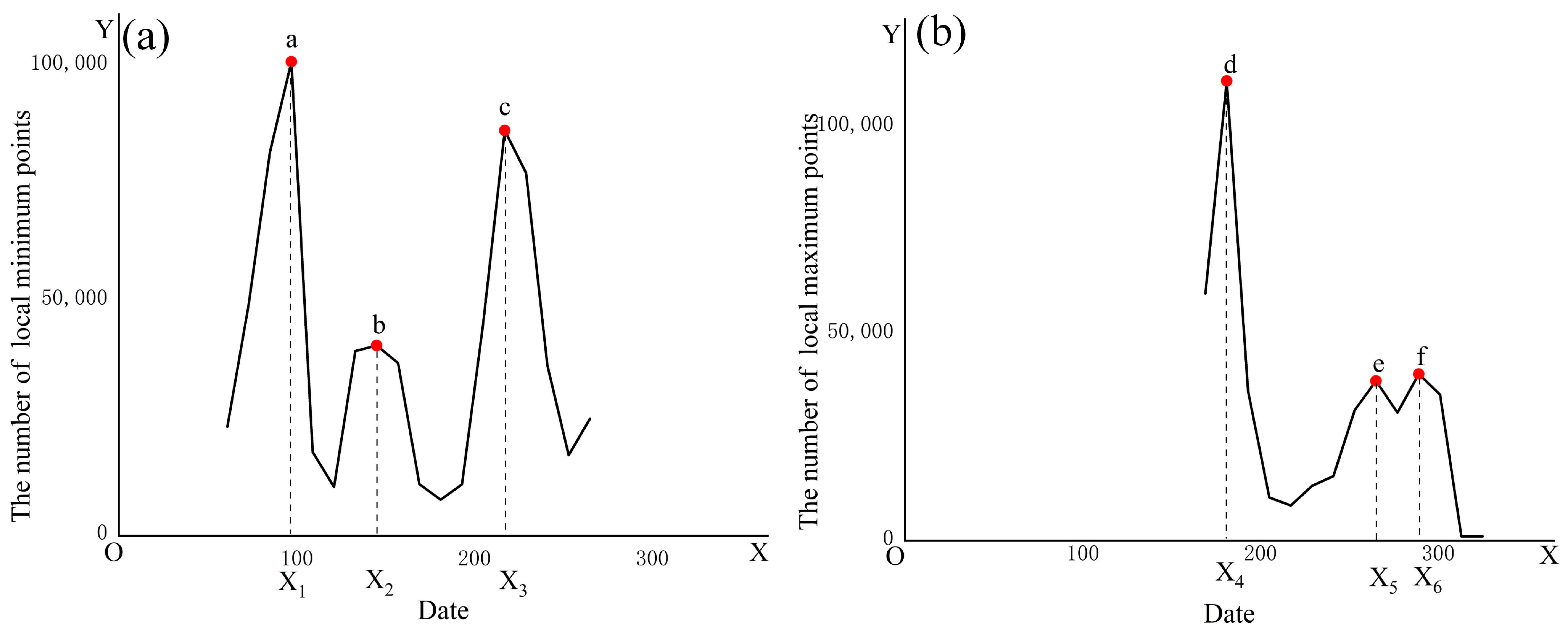
As shown in Figure 8, out of a total of 3138 pixels in 20 paddy fields, 697 pixels were identified as rice samples extracted by the dynamic threshold method. Figure 9 shows that the spatial distribution of rice samples extracted by the dynamic threshold method tends to be consistent with that of rice mapping by Auto-RMVPF (Figure 10c). These rice samples are distributed across the entire study area. As a result, the rice samples extracted by the dynamic threshold method can provide the representative phenological information about rice in the study area. However, some non-rice pixels are misclassified as rice samples, primarily located in the southern part of the study area near the South China Sea. For instance, many aquatic plants in the south, whose backscattering curves are similar to those of rice, are misclassified as rice. However, these misclassifications have little effect on the extraction of the phenological period because the number of misclassified pixels occupies a small proportion of the whole sample data. When using mathematical statistics to extract rice phenology, if the dates corresponding to the extreme points ( p 1 and p 2 , as shown in Figure 5) of the VH backscattering coefficient of incorrectly extracted rice samples are not equal to the dates of x1, x2, x3, x4, x5, or x6 corresponding to the extreme points of a, b, c, d, e, or f in Figure 11, they will be filtered out so that the results are not affected. In conclusion, rice samples extracted by the dynamic threshold method provide an important foundation for extracting phenological information.

4.2. Rice Phenological-Period Extraction

Figure 11 shows the results of rice phenology extracted by the second-order difference method. In this part, the local minimum and local maximum points in the VH backscattering curve are extracted by referring to the scattering mechanism of extracted rice samples. The local minimum point ( p 1 in Figure 5b) is considered the transplanting date, and the local maximum point ( p 2 in Figure 5b) is considered the harvest date of the rice. The number of minimum and maximum points (such as p 1 , p 2 ) are counted statistically and form a curve in which the date is on the X-axis and the number of extreme points is on the Y-axis, as shown in Figure 11. Smoothing the curve with a Savitzky–Golay filter helps to identify the local maximum points, such as points a, b, c, d, e, and f, in Figure 11. Then, we identify the dates x1, x2, x3, x4, x5, and x6 in Figure 11 that correspond to the local maximum points. The dates corresponding to the local maximum points (a, b, c) in Figure 11a are considered the transplanting dates of early rice, single rice, and late rice, respectively. Similarly, the dates corresponding to the local maximum points (d, e, f) in Figure 11b are considered the maturity dates of early rice, single rice, and late rice, respectively.
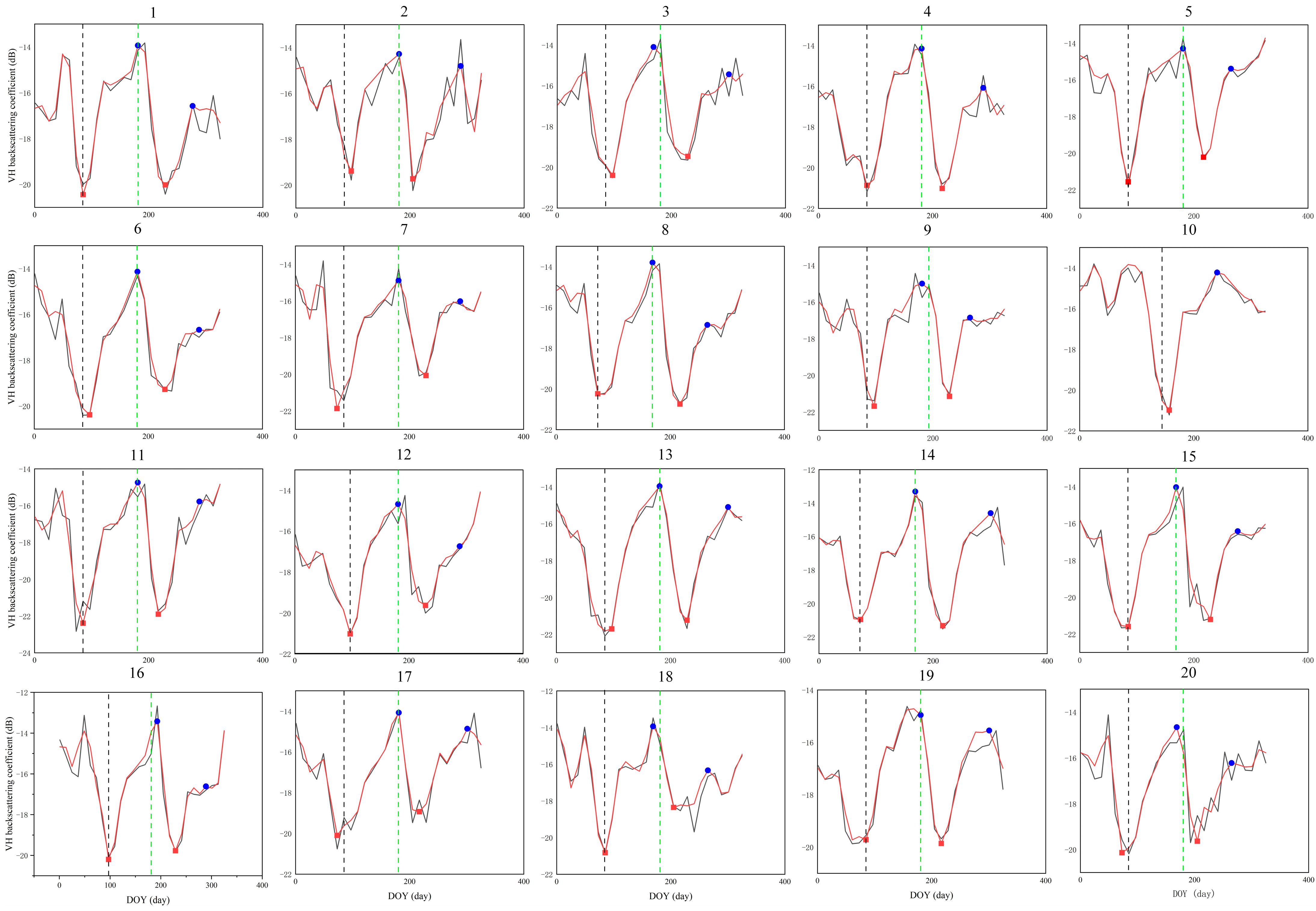
Figure 12 shows the phenological dates of 20 paddy fields. The transplanting and harvest dates for rice vary due to the differences in crop growth and the farmer’s decisions. Based on an analysis of the field survey data from 20 paddy fields, the transplanting dates for early rice are concentrated on DOY73, DOY85, and DOY97, while the harvest dates are concentrated on DOY169, DOY181, and DOY193. The transplanting date for single cropping rice is DOY145.
As shown in Figure 12, the rice phenological-period dates extracted by the second-order difference method are compared with the field survey data. For 11 out of the 20 paddy fields, the early rice transplanting dates are consistent with the field survey results. However, for the remaining 9 paddy fields, the early rice transplanting dates are more than 12 days than the dates obtained from the field survey. The reason for this discrepancy is that some rice paddy fields have little water or even bare soil surfaces during the transplanting period, resulting in a higher backscattering coefficient at that time. Regarding the extracted harvest dates for early rice, 14 paddy fields are consistent with the field survey results. The remaining 5 paddy fields have an error of 12 days. The main reasons for this error are that some rice fields have relatively high residual stubble after harvest, and mechanical harvesting can result in many wheel marks and disorganized rice stubble in the plots. This leads to a large backscattering coefficient for the paddy field.
Although the transplanting and harvest dates extracted for some paddy fields using the second-order difference method differ from the field survey dates by more or less than 12 days, this difference has little impact on the thresholds (e.g., T3, T4, T5, T6, T7, T8) of the slope of the VH backscattering curve. The reason for this is that the improved ARM-SARFS method calculates the slope of the VH backscattering curve over a large window, and the decision tree is not sensitive to the thresholds [2].

4.3. Noise Removal by Farmland Mask and Median Filter

The farmland mask is obtained from the 2019 Esri 10-Meter Land Cover, which is a public dataset published by Esri. The farmland mask is used to avoid the interference of non-farmland features on the identification results of rice mapping.
The effect of the median filter is mainly affected by the size of the filter window. In this study, the window size of the median filter is selected as five based on the analysis of the filter window size presented in Section 5.3.
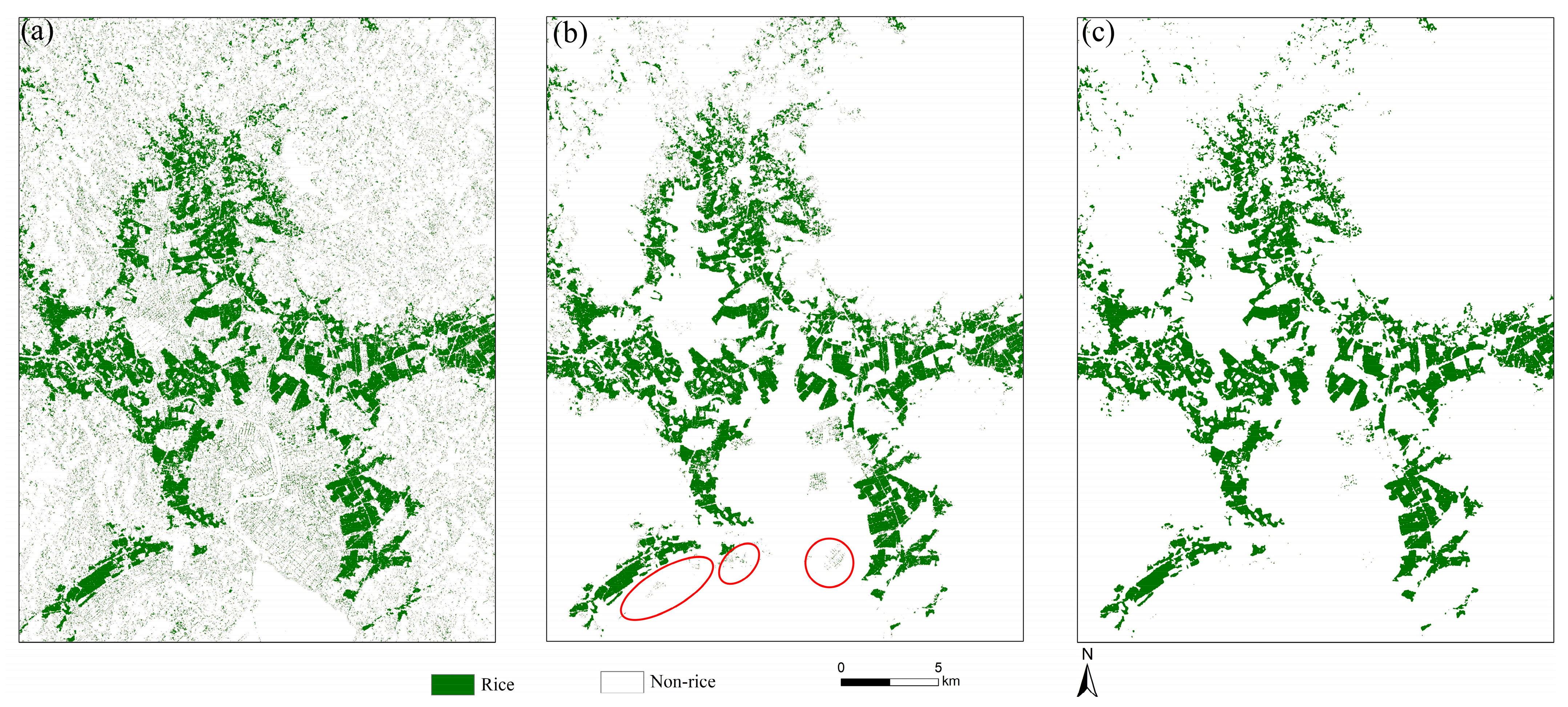
The results without the farmland mask and median filter exhibit a significant amount of noise, as shown in Figure 10a. After applying the farmland mask, a large amount of noise is eliminated, but some noise points remain, as shown in Figure 10b. The final results obtained after applying both the farmland mask and median filter show that the noise points have been largely eliminated, as shown in Figure 10c. It has a suitable effect on reducing noise in the study areas. Compared to Figure 10a, the number of noise points in Figure 10c is significantly reduced after processing with the farmland mask and median filter.

4.4. Rice Mapping

Figure 10c shows the spatial distribution map of rice in Taishan County, Guangdong Province, obtained by the Auto-RMVPF method. It has an overall accuracy of 95.0%, with an F 1 score of 0.913. As shown in Figure 10c, rice is mainly grown in the central area of Taishan County, and this is mainly due to the region being primarily plain, surrounded by mountains on three sides, and facing the South China Sea in the south. Its flat terrain and abundant water resources in this region provide favorable conditions for mechanized cultivation and management, making it suitable for large-scale rice cultivation. Rice is also sporadically distributed in the small fields in the mountains area. Most of the rice in these areas is planted by small-scale farmers, which is challenging to carry out large-scale rice planting due to the restrictions of many factors (e.g., large topographic relief, limited water resources, and low degree of mechanization). In conclusion, the Auto-RMVPF method based on time-series Sentinel-1A images has great potential for rice mapping, which contributes greatly to accurate crop management and monitoring.

5. Discussion

5.1. Temporal Feature of Sentinel-1A Backscatter for Rice

The VH backscattering coefficient decreases significantly on the transplanting date (Figure 12). The reason is that the early rice of double-cropping is first sown and then flooded in mid-February (DOY40) and transplanted in late March or early April (DOY90). During this period, the paddy field is usually a mixture of water, soil, and seedlings, with the water occupying a large proportion, which leads to a decline in the surface roughness of land and a small part of the incident wave scattered with the water surface. Therefore, the VH backscattering coefficient is lower than at other periods.
After transplanting, the VH backscattering coefficient gradually increases and reaches its peak (Figure 12). The reason is that rice grows until it matures in late June or early July (DOY180). During this period, the rice plants began to develop and overgrow under suitable water, light, and heat conditions. The number of leaves gradually increased, the area of the leaves expanded, and the rice plants spread out in the paddy field until the whole paddy field was covered. In this case, there is secondary and bulk scattering in the paddy fields. Consequently, the VH backscattering coefficient gradually increases until the rice is harvested.
At the mature period of rice, the VH backscattering coefficient decreased slightly. When rice matures, it enters the harvest period (Figure 12). After the rice is harvested, the VH backscattering coefficient of the paddy field tends to decrease. However, it does not decrease to a meager value because there is still residual stubble in some paddy fields after rice harvesting.

5.2. The Effect of Noise Removal through Different Filters

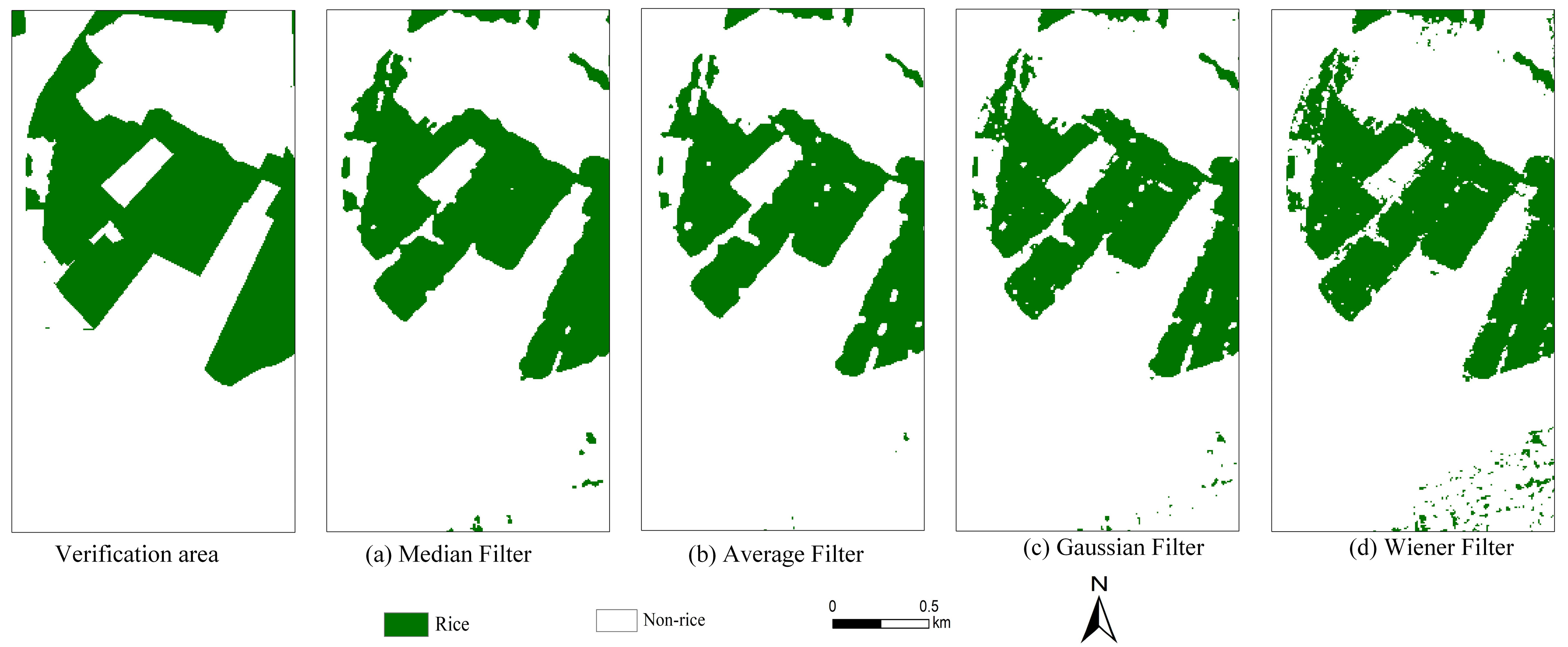
Many filters are effective at removing noise from images. In this section, we selected the median filter, average filter, Gaussian filter, and Wiener filter to post-process the classification results of rice, as shown in Figure 13. The precision assessment indexes of their results are compared, as shown in Table 1.
The overall accuracies of median filtering, mean filtering, Gaussian filtering, and Wiener filtering were 95.0%, 93.4%, 93.6%, and 93.7%, respectively. Although the differences in accuracy were small, median filtering has relatively less noise and was able to identify regular rice fields, as shown in Figure 13. Therefore, in this experiment, the median filter is selected to remove noise based on the rice classification result.

5.3. The Different Window Size Settings of the Median Filter

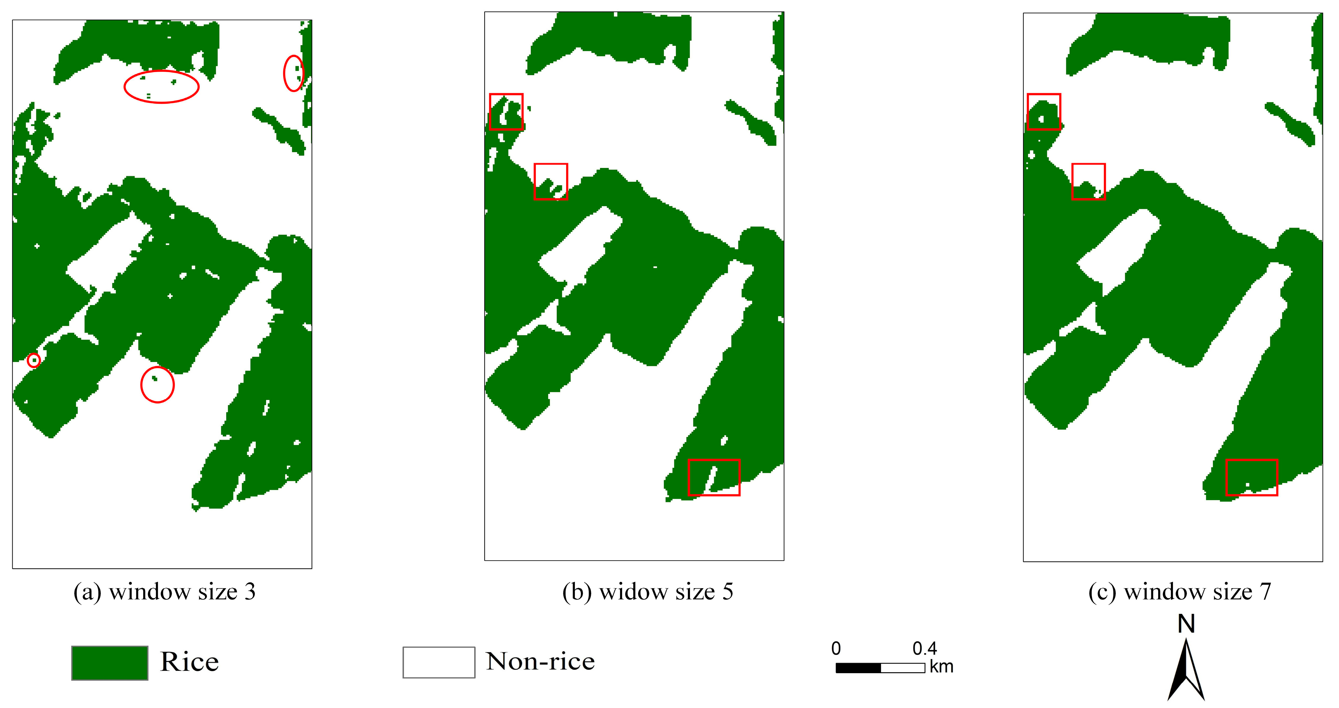
The effectiveness of the median filter is mainly affected by the size of the filter window. In order to determine the optimal filter window size, the influence of different filter window sizes is discussed in the experimental results. Windows with sizes 3, 5, and 7 are selected for experiments. The various assessment indexes of different window sizes are shown in Table 2. When the window size is 3, the overall accuracy is 94.5%. The pixels misclassified as rice cannot be removed entirely, as shown in the red circle and rectangle of Figure 14a, due to the large proportion of noise and the small window range. When the window size is 7, the overall accuracy is 95.4%. Non-rice pixels will also be misclassified as rice due to the large window range. Although it has a suitable effect on pixels misclassified as rice, the boundary information of paddy fields cannot be well protected, as shown in the red rectangle of Figure 14c. When the window size is 5, the overall accuracy is 95%. The boundary information of paddy fields can be well protected while the removal of noises is carried out, as shown in the red rectangle of Figure 14b. Therefore, a window size of 5 is used for the median filter in this study.

5.4. Comparison of Auto-RMVPF with Other Rice-Mapping Methods

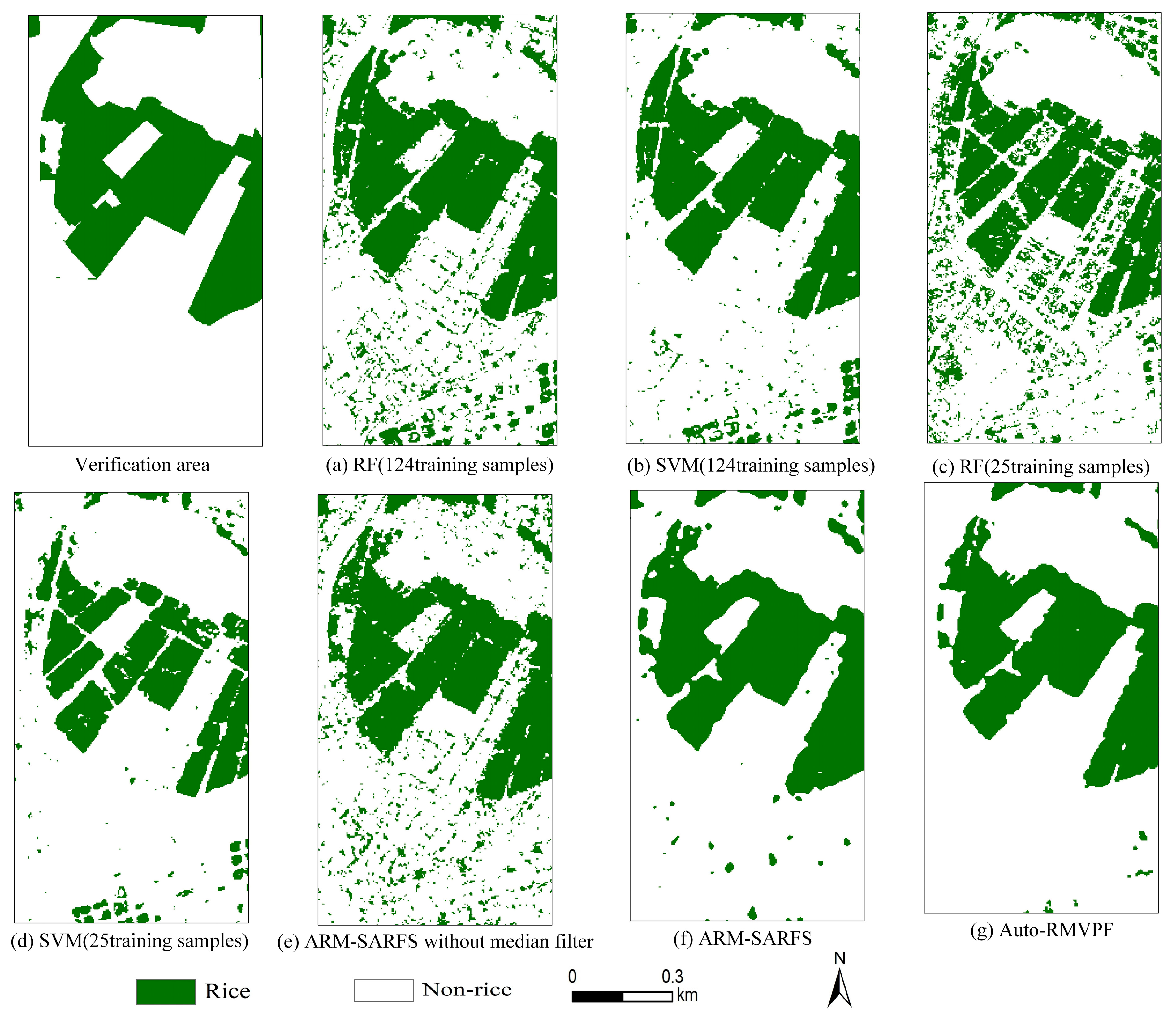
At present, there are many rice-mapping methods. Among these methods, two mainstream methods have been mostly explored and investigated in recent years, namely the phenology-based and machine learning (ML)-based methods. Hence, ARM-SARFS (a phenology-based method), random forest (RF), and support vector machine (SVM) (two classical ML-based methods) are used for comparison of Auto-RMVPF. The RF and SVM are supervised classification methods. The number of training samples greatly affects the experimental results. In this study, we selected two sets of training samples with different sizes to train the RF and SVM models. In addition, the result of the ARM-SARFS method with median filtering is also compared with that of the ARM-SARFS method without median filtering. Rice mappings of RF, SVM, ARM-SARFS without median filtering, ARM-SARFS with median filtering, and Auto-RMVPF methods are shown in Figure 15.
Figure 16 shows the rice classification of the verification region by the Auto-RMVPF method and the other methods. From the results of RF (Figure 16a,c) and ARM-SARFS without median filtering (Figure 16e), the ponds are misclassified as rice, which leads to lots of noise. In addition, due to the limited number of samples, RF and SVM with a small number of training samples could not identify all pixels of rice in the paddy field. Hence, the paddy field is relatively fragmented, as shown in Figure 16c,d. Although increasing the number of training samples can improve the ability of the SVM model to accurately classify rice and make the field more regular, there are still instances where ponds are misclassified as rice, as shown in Figure 16b. However, most noises are filtered by ARM-SARFS with median filtering (Figure 16f), so the results are more accurate. Auto-RMVPF can automatically extract a large number of rice samples (Figure 9) and then automatically extract the phenological dates of the rice for rice mapping, which is not limited by sample quantity and crop calendar data. Moreover, the result of Auto-RMVPF is more consistent with the actual situation in the verification area (Figure 16). Therefore, the Auto-RMVPF method is more suitable for mapping rice automatically.
Table 3 compares various assessment indexes between the Auto-RMVPF and other rice-mapping methods. The overall accuracy of the Auto-RMVPF method reached 95.0% (Kappa = 0.878), and the F 1 score is 0.913. The accuracy of producers and users in the study area is above 87%, indicating that the results of Auto-RMVPF are relatively accurate.
The accuracy of the other two machine-learning methods is lower than that of Auto-RMVPF, and the OA decreased by 2.8–12.2% ( F 1 score decreased by 0.042–0.189). Among them, the UA of the RF (25 training samples and 124 training samples) method is relatively low, indicating that the possibility of rice misclassification in this method is high. Moreover, the PA of the SVM (25 training samples) method is also low, indicating that the method has a high possibility of missing classification in rice. SVM is a supervised classification method that is well-suited for a small sample number. As the number of training samples increases, both the UA and PA of the SVM (124 training samples) can achieve suitable levels of accuracy. RF is a supervised classification method that relies on the number of training samples. When the number of training samples is small, the UA and PA of the RF (25 training samples) are low.
However, the overall accuracy of the RF and SVM methods for rice classification in the verification area reached more than 82%. The result of RF (Figure 15a,c) showed that some non-rice pixels are misclassified as rice pixels. The result of the SVM (25 training samples) and RF (25 training samples) showed that the rice distribution is relatively fragmented (Figure 15c,d).
Compared with the ARM-SARFS method without median filtering (in Figure 15e), the ARM-SARFS method with median filtering (Figure 15f) improved the OA by 4.3% ( F 1 score by 0.063) (Table 3), indicating that the median filter has a suitable effect on the removal of rice misclassification. Auto-RMVPF (Figure 15g) and ARM-SARFS with median filter have little difference in OA, Kappa coefficient, and F 1 score (Table 3). It is fully demonstrated that the phenological periods automatically extracted by the Auto-RMVPF method are in suitable agreement with the phenological periods that are used for the ARM-SARFS method from the existing crop calendar data. Furthermore, the Auto-RMVPF method can also achieve higher accuracy in rice mapping.
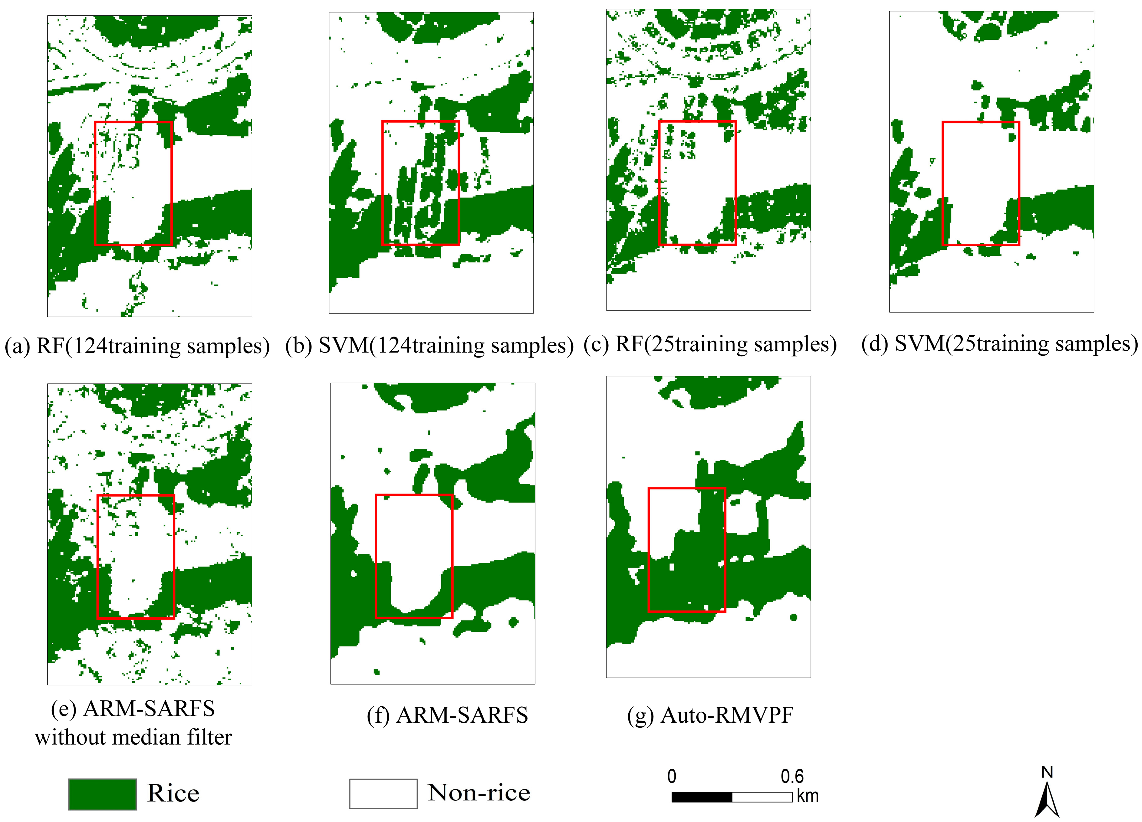
However, neither the classical ML-based methods of RF (25 training samples and 124 training samples) and SVM (25 training samples) nor the phenology-based ARM-SARFS method could identify the single-rice growing region in the study area, as shown in Figure 17a,c–f). As the number of training samples increases, the ability of the SVM (124 training samples) to classify rice accurately improves significantly. However, due to the limited number of training samples for single rice, the model is only able to identify fragmented single-rice fields, as shown in Figure 17b. Both RF and SVM methods require a large number of single-rice samples to train the model to identify single rice. However, the planting area of single rice in the study area is so small that it is difficult to obtain enough samples of single rice. Although the ARM-SARFS method does not require training samples, it relies on crop calendar data. The ARM-SARFS method also cannot identify the planting area of single rice because it has only the phenological data of double rice for the study area. It is worth noting that the Auto-RMVPF method does not depend on the crop calendar. It can automatically extract a large number of samples of single rice and double rice simultaneously as training data to extract the rice phenology for rice mapping. Therefore, the Auto-RMVPF method can identify both single rice and double rice, as shown in Figure 17g, showing its superiority in rice mapping.

5.5. The Suitability of Auto-RMVPF for Different Terrains

According to the rice mapping of Auto-RMVPF shown in Figure 15g, although the overall classification is suitable, there are still instances of rice misclassification in some areas of the study area. These misclassification cases mainly occurred in the northwestern and southern regions. The northwest region is primarily wooded and mountainous, which is not conducive to mapping rice. The southern part of the study area is adjacent to the South China Sea, and there are some shallows and wetlands because of sediment accumulation. In the transplanting period of rice, the backscattering coefficient of aquatic plants is relatively low due to the high water content. By early April, the backscattering coefficient of aquatic plants gradually increased as vegetation grew, similar to the backscatter of rice. Therefore, they will show similar features in the time-series VH backscattering curve, which increases the difficulty of the classification of rice. Although the farmland mask has successfully extracted most of the farmland within the study area, it has also inevitably included some non-farmland areas. As a result, these instances of misclassification have not been completely eliminated.
In the central region of the study area (Figure 15g), the classification of rice is less noisy. This is because the rice fields in these areas are large and regular in shape, and the VH backscattering curve of rice is also significantly different from those of other planted crops, thus increasing the separability.
In conclusion, the ability of the Auto-RMVPF method to classify rice varies in different terrains. Suitable classification can be achieved in large rice-planting areas with regular-shaped paddy fields and fewer miscellaneous plants. In contrast, there is room for improvement in small rice-planting areas and paddy fields with complex land-cover types.

5.6. Advantages of the Auto-RMVPF Method

When considering rice mapping or other remote-sensing applications, it is always preferred to choose the method with the lowest cost or minimum input and the best results. Traditional machine-learning methods can achieve suitable accuracy for rice mapping in some areas due to a large training set of data to train the model. Thus, it requires a colossal workforce and material resources to collect training set data before the experiment. However, abundant rice samples are extracted automatically by the dynamic threshold method, which is an important part of the Auto-RMVPF method based on the temporal VH backscattering coefficient curve of rice, avoiding the tedious work of manual sample collection.
The geometric structure of rice changes greatly during its growth periods, and the phenological information of rice is crucial for classification. To better extract the phenological features of rice from the time-series data, smoothing the data is an indispensable step. However, many smoothing methods have been used for time-series data, such as wavelet transform and Kalman filter. These methods can achieve suitable results in smoothing time-series data but are not suitable for rice. This is because these methods only focus on smoothing the data, and they ignore the changes in the data caused by unexpected conditions. For instance, rainfall events may cause a temporary decline in the VH backscattering coefficient of rice (e.g., f d in Figure 5b). If only one filter is used to smooth the temporal VH backscattering curve of rice, it may lead to data loss at some critical time points and then miss the phenological information about rice. Therefore, the SG filter is used in this study to smooth the rice temporal VH backscattering curve. Additionally, the time filter [28] is also selected to filter out the decline data less than 40 days in the temporal VH backscattering curve (f(d) in Figure 5b). It can avoid the loss of phenological information due to unexpected events.
The Auto-RMVPF method is not sensitive to the threshold value of T1, T2, T3, T4, T5, T6, T7, and T8. T1, T3, T4, T5, and T6 are fixed every year in different regions [2]. T2 in central and southern China is empirically set to −17 dB, and in northern China is set to −20 dB [2]. The reason is that VH backscatter values in northern China are lower than that in southern China [2]. T7 and T8 can be set to −0.009 and 0.02, respectively, based on the analysis of VH backscattering coefficients, resulting in an overall accuracy of 95%. In addition, both T7 and T8 can be set to 0 with an overall accuracy of 94.6% (Table 4). The overall accuracies of the two sets are slightly different. Therefore, T3, T4, T5, T6, T7, and T8, all of which are set to 0, will be studied further in the absence of training samples.
The ARM-SARFS method can achieve high classification accuracy without the need for training samples, and satisfactory results can be obtained in the areas of different rice-planting types, proving the method’s robustness [2]. However, it can only be used for rice mapping in areas with crop calendar data due to the need for manually setting rice phenological periods. The accuracy of rice mapping is highly dependent on the accuracy of the crop calendar. Setting manually driven phenological periods of rice, the ARM-SARFS method is unable to identify single rice in areas where double rice is primarily planted, as shown in Figure 17e,f. The reason is that only the phenological data for double rice could be obtained from the local crop calendar but the lack of phenological data for single rice. When rice phenological periods are manually set for rice mapping, the lack of phenological information on single rice leads to the inability to identify single rice. However, the phenological information of both can be obtained simultaneously by the improved ARM-SARFS method, in which double- and single-rice samples are automatically extracted. For instance, the paddy fields planted with single rice have been identified, as shown in Figure 17g. The improved ARM-SARFS method can make rice mapping by automatically extracting phenological data based on the scattering mechanism of rice. As a result, spatial distribution maps of rice can be obtained even in areas without crop calendar data.

6. Conclusions

In this study, we designed an automatic rice-mapping method called Auto-RMVPF to distinguish rice from other land-cover types based on the Sentinel-1A time-series data and the phenological features of rice. This method included the dynamic threshold method for extracting rice samples, the second-order difference method for extracting rice phenological periods, the improved ARM-SARFS method, which does not need to set the phenological dates for rice mapping manually, and the farmland mask and median filter for removing noise. We tested its capacity in Taishan County and compared its performance with three existing methods (two classical ML-based methods and a phenology-based method). Results show that the Auto-RMVPF can provide accurate rice mapping with an overall accuracy of 95.0%, which is better than RF with an overall accuracy of 82.8% (25 training samples) and 88.3% (124 training samples), SVM with an overall accuracy of 89.9% (25 training samples) and 92.2% (124 training samples), and ARM-SARFS with an overall accuracy of 89.9%. The proposed Auto-RMVPF method has several advantages: (1) abundant rice samples are extracted automatically by the dynamic threshold method without manual sample collection; (2) the rice phenological periods are automatically extracted by the second-order difference method to obtain satisfactory accuracy for rice mapping in areas without crop calendar data; (3) the threshold values of the decision tree are insensitive to the identification of rice varieties with the variation of soil water content. Therefore, this method has broad application prospects for automatic rice mapping, especially for cloudy regions with limited optical remote-sensing data.

Author Contributions

Conceptualization, G.T., H.L. and H.Y.; data curation, H.Y., Q.J. and N.L.; investigation, G.T., N.L., Z.G. and H.Y.; methodology, G.T., H.L. and H.Y.; supervision, B.Q., J.Z. and N.L.; writing—original draft, G.T., N.L. and H.Y.; writing—review and editing, G.T., H.L. and H.Y. All authors have read and agreed to the published version of the manuscript.

Funding

This research was funded by the National Natural Science Foundation of China (42101386), the College Key Research Project of Henan Province (22A520021), the Plan of Science and Technolo-gy of Henan Province (222102110439,232102211043), the Key Laboratory of Natural Resources Monitoring and Regulation in Southern Hilly Region, Ministry of Natural Resources of the People’s Republic of China (NRMSSHR2022Z01), Plan of Science and Technology of Department of Natural Resources of Hunan Province (2022-08) and the Key Laboratory of Land Satellite Remote Sensing Application, Ministry of Natural Resources of the People’s Republic of China (KLSMNR-202302).

Data Availability Statement

All data and models presented in this study are available.

Acknowledgments

Thanks to all anonymous reviewers and editors for their comments and suggestions that made the article’s content more rigorous and meaningful. At the same time, thanks to the ESA for providing the multi-temporal Sentinel-1A SAR data for agriculture applications.

Conflicts of Interest

The authors declare no conflict of interest.

References

  1. De Bernardis, C.G.; Vicente-Guijalba, F.; Martinez-Marin, T.; Lopez-Sanchez, J.M. Particle filter approach for crop phenological stage estimation using time series of NDVI images. In Proceedings of the 2015 IEEE International Geoscience and Remote Sensing Symposium (IGARSS), Milan, Italy, 26–31 July 2015. [Google Scholar]
  2. Zhan, P.; Zhu, W.; Li, N. An automated rice mapping method based on flooding signals in synthetic aperture radar time series. Remote Sens. Environ. 2021, 252, 112112. [Google Scholar] [CrossRef]
  3. Zhang, G.; Xiao, X.; Dong, J.; Xin, F.; Zhang, Y.; Qin, Y.; Moore III, B. Fingerprint of rice paddies in spatial–temporal dynamics of atmospheric methane concentration in monsoon Asia. Nat. Commun. 2020, 11, 554. [Google Scholar] [CrossRef]
  4. Linquist, B.A.; Adviento-Borbe, M.A.; Pittelkow, C.M.; van Kessel, C.; van Groenigen, K.J. Fertilizer management practices and greenhouse gas emissions from rice systems: A quantitative review and analysis. Field Crops Res. 2012, 135, 10–21. [Google Scholar] [CrossRef]
  5. Li, N.; Li, H.; Zhao, J.; Guo, Z.; Yang, H. Mapping winter wheat in Kaifeng, China using Sentinel-1A time-series images. Remote Sens. Lett. 2022, 13, 503–510. [Google Scholar] [CrossRef]
  6. Li, H.; Lu, J.; Tian, G.; Yang, H.; Zhao, J.; Li, N. Crop Classification Based on GDSSM-CNN Using Multi-Temporal RADARSAT-2 SAR with Limited Labeled Data. Remote Sens. 2022, 14, 3889. [Google Scholar] [CrossRef]
  7. Khatami, R.; Mountrakis, G.; Stehman, S.V. A meta-analysis of remote sensing research on supervised pixel-based land-cover image classification processes: General guidelines for practitioners and future research. Remote Sens. Environ. 2016, 177, 89–100. [Google Scholar] [CrossRef]
  8. Weiss, M.; Jacob, F.; Duveiller, G. Remote sensing for agricultural applications: A meta-review. Remote Sens. Environ. 2020, 236, 111402. [Google Scholar]
  9. Yang, S.; Shen, S.; Li, B.; Le Toan, T.; He, W. Rice mapping and monitoring using ENVISAT ASAR data. IEEE Geosci. Remote Sens. Lett. 2008, 5, 108–112. [Google Scholar] [CrossRef]
  10. Chauhan, S.; Darvishzadeh, R.; Boschetti, M.; Pepe, M.; Nelson, A. Remote sensing-based crop lodging assessment: Current status and perspectives. ISPRS J. Photogramm. Remote Sens. 2019, 151, 124–140. [Google Scholar] [CrossRef]
  11. Park, S.; Im, J.; Park, S.; Yoo, C.; Han, H.; Rhee, J. Classification and Mapping of Paddy Rice by Combining Landsat and SAR Time Series Data. Remote Sens. 2018, 10, 447. [Google Scholar] [CrossRef]
  12. Dong, J.; Xiao, X. Evolution of regional to global paddy rice mapping methods: A review. ISPRS J. Photogramm. Remote Sens. 2016, 119, 214–227. [Google Scholar] [CrossRef]
  13. Yang, H.; Li, H.; Wang, W.; Li, N.; Zhao, J.; Pan, B. Spatio-Temporal Estimation of Rice Height Using Time Series Sentinel-1 Images. Remote Sens. 2022, 14, 546. [Google Scholar] [CrossRef]
  14. Lopez-Sanchez, J.M.; Cloude, S.R.; Ballester-Berman, J.D. Rice phenology monitoring by means of SAR polarimetry at X-band. IEEE Trans. Geosci. Remote Sens. 2011, 50, 2695–2709. [Google Scholar] [CrossRef]
  15. Lopez-Sanchez, J.M.; Vicente-Guijalba, F.; Erten, E.; Campos-Taberner, M.; Garcia-Haro, F.J. Retrieval of vegetation height in rice fields using polarimetric SAR interferometry with TanDEM-X data. Remote Sens. Environ. 2017, 192, 30–44. [Google Scholar] [CrossRef]
  16. Lopez-Sanchez, J.M.; Vicente-Guijalba, F.; Ballester-Berman, J.D.; Cloude, S.R. Polarimetric response of rice fields at C-band: Analysis and phenology retrieval. IEEE Trans. Geosci. Remote Sens. 2013, 52, 2977–2993. [Google Scholar] [CrossRef]
  17. Mascolo, L.; Lopez-Sanchez, J.M.; Vicente-Guijalba, F.; Nunziata, F.; Migliaccio, M.; Mazzarella, G. A complete procedure for crop phenology estimation with PolSAR data based on the complex Wishart classifier. IEEE Trans. Geosci. Remote Sens. 2016, 54, 6505–6515. [Google Scholar] [CrossRef]
  18. Zhou, X.; Zheng, H.B.; Xu, X.Q.; He, J.Y.; Ge, X.K.; Yao, X.; Cheng, T.; Zhu, Y.; Cao, W.X.; Tian, Y.C. Predicting grain yield in rice using multi-temporal vegetation indices from UAV-based multispectral and digital imagery. ISPRS J. Photogramm. Remote Sens. 2017, 130, 246–255. [Google Scholar] [CrossRef]
  19. Clauss, K.; Ottinger, M.; Leinenkugel, P.; Kuenzer, C. Estimating rice production in the Mekong Delta, Vietnam, utilizing time series of Sentinel-1 SAR data. Int. J. Appl. Earth Obs. Geoinf. 2018, 73, 574–585. [Google Scholar] [CrossRef]
  20. Gumma, M.K.; Thenkabail, P.S.; Maunahan, A.; Islam, S.; Nelson, A. Mapping seasonal rice cropland extent and area in the high cropping intensity environment of Bangladesh using MODIS 500 m data for the year 2010. ISPRS J. Photogramm. Remote Sens. 2014, 91, 98–113. [Google Scholar] [CrossRef]
  21. Nuarsa, I.W.; Nishio, F.; Hongo, C.; Mahardika, I.G. Using variance analysis of multitemporal MODIS images for rice field mapping in Bali Province, Indonesia. Int. J. Remote Sens. 2012, 33, 5402–5417. [Google Scholar] [CrossRef]
  22. Peng, D.; Huete, A.R.; Huang, J.; Wang, F.; Sun, H. Detection and estimation of mixed paddy rice cropping patterns with MODIS data. Int. J. Appl. Earth Obs. Geoinf. 2011, 13, 13–23. [Google Scholar] [CrossRef]
  23. Qin, Y.; Xiao, X.; Dong, J.; Zhou, Y.; Zhu, Z.; Zhang, G.; Du, G.; Jin, C.; Kou, W.; Wang, J.; et al. Mapping paddy rice planting area in cold temperate climate region through analysis of time series Landsat 8 (OLI), Landsat 7 (ETM+) and MODIS imagery. ISPRS J. Photogramm. Remote Sens. 2015, 105, 220–233. [Google Scholar] [CrossRef] [PubMed]
  24. Guan, X.; Huang, C.; Liu, G.; Meng, X.; Liu, Q. Mapping Rice Cropping Systems in Vietnam Using an NDVI-Based Time-Series Similarity Measurement Based on DTW Distance. Remote Sens. 2016, 8, 19. [Google Scholar] [CrossRef]
  25. Li, P.; Xiao, C.; Feng, Z. Mapping rice planted area using a new normalized EVI and SAVI (NVI) derived from Landsat-8 OLI. IEEE Geosci. Remote Sens. Lett. 2018, 15, 1822–1826. [Google Scholar] [CrossRef]
  26. Kontgis, C.; Schneider, A.; Ozdogan, M. Mapping rice paddy extent and intensification in the Vietnamese Mekong River Delta with dense time stacks of Landsat data. Remote Sens. Environ. 2015, 169, 255–269. [Google Scholar] [CrossRef]
  27. Xiao, X.; Boles, S.; Liu, J.; Zhuang, D.; Frolking, S.; Li, C.; Moore III, B. Mapping paddy rice agriculture in southern China using multi-temporal MODIS images. Remote Sens. Environ. 2005, 95, 480–492. [Google Scholar] [CrossRef]
  28. Xu, S.; Zhu, X.; Chen, J.; Zhu, X.; Duan, M.; Qiu, B.; Wan, L.; Tan, X.; Xu, Y.; Cao, R. A robust index to extract paddy fields in cloudy regions from SAR time series. Remote Sens. Environ. 2023, 285, 113374. [Google Scholar] [CrossRef]
  29. Gómez, C.; White, J.C.; Wulder, M.A. Optical remotely sensed time series data for land cover classification: A review. ISPRS J. Photogramm. Remote Sens. 2016, 116, 55–72. [Google Scholar] [CrossRef]
  30. Shao, Y.; Fan, X.; Liu, H.; Xiao, J.; Ross, S.; Brisco, B.; Brown, R.; Staples, G. Rice monitoring and production estimation using multitemporal RADARSAT. Remote Sens. Environ. 2001, 76, 310–325. [Google Scholar] [CrossRef]
  31. Zhang, X.; Wu, B.; Ponce-Campos, G.E.; Zhang, M.; Chang, S.; Tian, F. Mapping up-to-date paddy rice extent at 10 m resolution in china through the integration of optical and synthetic aperture radar images. Remote Sens. 2018, 10, 1200. [Google Scholar] [CrossRef]
  32. Jiao, X.; Kovacs, J.M.; Shang, J.; McNairn, H.; Walters, D.; Ma, B.; Geng, X. Object-oriented crop mapping and monitoring using multi-temporal polarimetric RADARSAT-2 data. ISPRS J. Photogramm. Remote Sens. 2014, 96, 38–46. [Google Scholar] [CrossRef]
  33. Lasko, K.; Vadrevu, K.P.; Tran, V.T.; Justice, C. Mapping double and single crop paddy rice with Sentinel-1A at varying spatial scales and polarizations in Hanoi, Vietnam. IEEE J. Sel. Top. Appl. Earth Obs. Remote Sens. 2018, 11, 498–512. [Google Scholar] [CrossRef]
  34. Bouvet, A.; Le Toan, T. Use of ENVISAT/ASAR wide-swath data for timely rice fields mapping in the Mekong River Delta. Remote Sens. Environ. 2011, 115, 1090–1101. [Google Scholar] [CrossRef]
  35. Fan, K.T.; Chen, Y.S.; Lin, C.W.; Tzeng, Y.C. Identification of rice paddy fields from multitemporal polarimetric SAR images by scattering matrix decomposition. In Proceedings of the 2015 IEEE International Geoscience and Remote Sensing Symposium (IGARSS), Milan, Italy, 26–31 July 2015. [Google Scholar]
  36. Hoang, H.K.; Bernier, M.; Duchesne, S.; Tran, Y.M. Rice mapping using RADARSAT-2 dual-and quad-pol data in a complex land-use Watershed: Cau River Basin (Vietnam). IEEE J. Sel. Top. Appl. Earth Obs. Remote Sens. 2016, 9, 3082–3096. [Google Scholar] [CrossRef]
  37. Miyaoka, K.; Maki, M.; Susaki, J.; Homma, K.; Noda, K.; Oki, K. Rice-planted area mapping using small sets of multi-temporal SAR data. IEEE Geosci. Remote Sens. Lett. 2013, 10, 1507–1511. [Google Scholar] [CrossRef]
  38. Thorp, K.R.; Drajat, D. Deep machine learning with Sentinel satellite data to map paddy rice production stages across West Java, Indonesia. Remote Sens. Environ. 2021, 265, 112679. [Google Scholar] [CrossRef]
  39. He, Z.; Li, S.; Wang, Y.; Dai, L.; Lin, S. Monitoring Rice Phenology Based on Backscattering Characteristics of Multi-Temporal RADARSAT-2 Datasets. Remote Sens. 2018, 10, 340. [Google Scholar] [CrossRef]
  40. Inoue, Y.; Sakaiya, E.; Wang, C. Capability of C-band backscattering coefficients from high-resolution satellite SAR sensors to assess biophysical variables in paddy rice. Remote Sens. Environ. 2014, 140, 257–266. [Google Scholar] [CrossRef]
  41. Li, H.; Fu, D.; Huang, C.; Su, F.; Liu, Q.; Liu, G.; Wu, S. An Approach to High-Resolution Rice Paddy Mapping Using Time-Series Sentinel-1 SAR Data in the Mun River Basin, Thailand. Remote Sens. 2020, 12, 3959. [Google Scholar] [CrossRef]
  42. Yang, L.; Huang, R.; Huang, J.; Lin, T.; Wang, L.; Mijiti, R.; Wei, P.; Tang, C.; Shao, J.; Li, Q.; et al. Semantic segmentation based on temporal features: Learning of temporal–spatial information from time-series SAR images for paddy rice mapping. IEEE Trans. Geosci. Remote Sens. 2021, 60, 4403216. [Google Scholar] [CrossRef]
  43. Wei, P.; Chai, D.; Lin, T.; Tang, C.; Du, M.; Huang, J. Large-scale rice mapping under different years based on time-series Sentinel-1 images using deep semantic segmentation model. ISPRS J. Photogramm. Remote Sens. 2021, 174, 198–214. [Google Scholar] [CrossRef]
  44. Xu, L.; Zhang, H.; Wang, C.; Wei, S.; Zhang, B.; Wu, F.; Tang, Y. Paddy rice mapping in thailand using time-series sentinel-1 data and deep learning model. Remote Sens. 2021, 13, 3994. [Google Scholar] [CrossRef]
  45. Lin, Z.; Zhong, R.; Xiong, X.; Guo, C.; Xu, J.; Zhu, Y.; Xu, J.; Ying, Y.; Ting, K.C.; Huang, J.; et al. Large-Scale Rice Mapping Using Multi-Task Spatiotemporal Deep Learning and Sentinel-1 SAR Time Series. Remote Sens. 2022, 14, 699. [Google Scholar] [CrossRef]
  46. Clauss, K.; Ottinger, M.; Künzer, C. Mapping rice areas with Sentinel-1 time series and superpixel segmentation. Int. J. Remote Sens. 2018, 39, 1399–1420. [Google Scholar] [CrossRef]
  47. Guo, Y.; Jia, X.; Paull, D.; Benediktsson, J.A. Nomination-favoured opinion pool for optical-SAR-synergistic rice mapping in face of weakened flooding signals. ISPRS J. Photogramm. Remote Sens. 2019, 155, 187–205. [Google Scholar] [CrossRef]
  48. Nguyen, D.B.; Gruber, A.; Wagner, W. Mapping rice extent and cropping scheme in the Mekong Delta using Sentinel-1A data. Remote Sens. Lett. 2016, 7, 1209–1218. [Google Scholar] [CrossRef]
  49. Bazzi, H.; Baghdadi, N.; El Hajj, M.; Zribi, M.; Minh, D.H.T.; Ndikumana, E.; Courault, D.; Belhouchette, H. Mapping Paddy Rice Using Sentinel-1 SAR Time Series in Camargue, France. Remote Sens. 2019, 11, 887. [Google Scholar] [CrossRef]
  50. Chen, J.; Lin, H.; Pei, Z. Application of ENVISAT ASAR data in mapping rice crop growth in Southern China. IEEE Geosci. Remote Sens. Lett. 2007, 4, 431–435. [Google Scholar] [CrossRef]
  51. Pan, B.; Zheng, Y.; Shen, R.; Ye, T.; Zhao, W.; Dong, J.; Ma, H.; Yuan, W. High Resolution Distribution Dataset of Double-Season Paddy Rice in China. Remote Sens. 2021, 13, 4609. [Google Scholar] [CrossRef]
  52. Fiorillo, E.; Di Giuseppe, E.; Fontanelli, G.; Maselli, F. Lowland Rice Mapping in Sédhiou Region (Senegal) Using Sentinel 1 and Sentinel 2 Data and Random Forest. Remote Sens. 2020, 12, 3403. [Google Scholar] [CrossRef]
  53. Yang, H.; Pan, B.; Li, N.; Wang, W.; Zhang, J.; Zhang, X. A systematic method for spatio-temporal phenology estimation of paddy rice using time series Sentinel-1 images. Remote Sens. Environ. 2021, 259, 112394. [Google Scholar] [CrossRef]
  54. Clauss, K.; Yan, H.; Kuenzer, C. Mapping paddy rice in China in 2002, 2005, 2010 and 2014 with MODIS time series. Remote Sens. 2016, 8, 434. [Google Scholar] [CrossRef]
  55. Rad, A.M.; Ashourloo, D.; Shahrabi, H.S.; Nematollahi, H. Developing an automatic phenology-based algorithm for rice detection using sentinel-2 time-series data. IEEE J. Sel. Top. Appl. Earth Obs. Remote Sens. 2019, 12, 1471–1481. [Google Scholar]
  56. Huang, H.; Gao, Z. The extraction of multiple cropping index of China based on NDVI time-series. In Proceedings of the SPIE Remote Sensing and Modeling of Ecosystems for Sustainability VIII, San Diego, CA, USA, 15 September 2011. [Google Scholar]
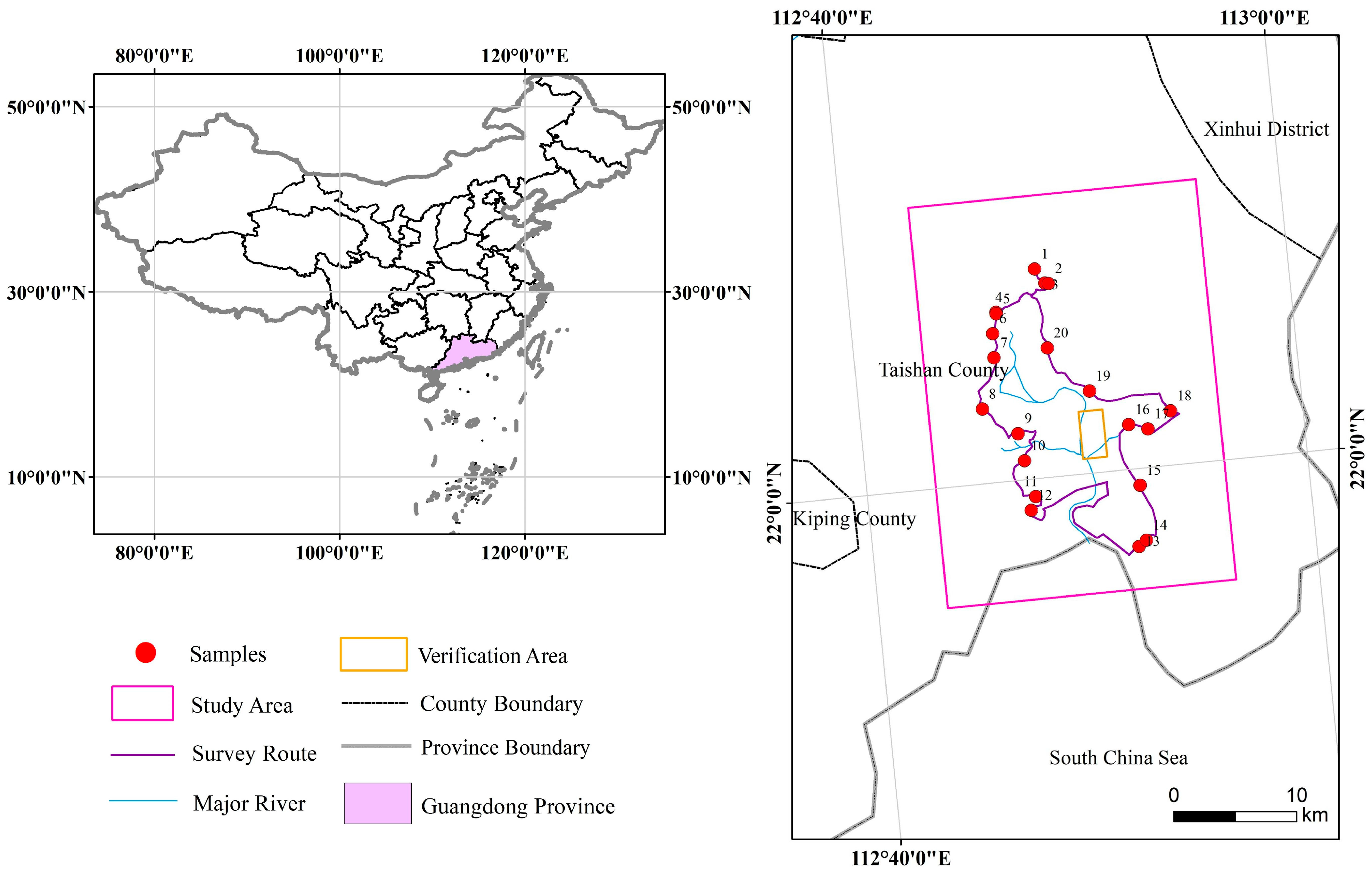
Figure 1. The location of the study area in Taishan County, Guangdong Province, China. Red points are the locations of each field survey. The purple line represents the route of the ground campaigns. The yellow box represents the verification area, and the pink box represents the study area.
Remotesensing 15 02785 g001
Figure 2. Rice cropping calendar and schedule of acquisitions organized as Sentinel images and ground campaigns. Black circles denote acquired Sentinel-1A images, and red crosses denote a lack of images. Black triangles denote the date of ground campaigns. There are no Sentinel-1A images with the acquisition date of 25 May 2019. The backscattering coefficients of rice for 25 May 2019 were calculated based on the mean value of backscattering coefficients for 13 May and 5 June 2019.
Remotesensing 15 02785 g002
Figure 3. VH backscattering coefficient curve of different land-cover types.
Remotesensing 15 02785 g003
Figure 4. The framework of the proposed Auto-RMVPF method. The rice samples extraction based on the dynamic threshold method. The rice phenological-period extraction based on the second-order method. The rice mapping based on the improved ARM-SARFS method.
Remotesensing 15 02785 g004
Figure 5. Filtering process of VH backscattering curve of rice. (a) SG filter; (b) Time filter.
Remotesensing 15 02785 g005
Figure 6. Process diagram of extracting local maximum and local minimum points from rice-growth curve. (a) The original VH band time series of single rice; (b) results of step 2; (c) results of step 3; (d) results of the final step, the red rectangle represents a growth period of rice (i.e., the growing period of rice).
Remotesensing 15 02785 g006
Figure 7. Schematic diagram of the principle of median filter.
Remotesensing 15 02785 g007
Figure 8. The rice samples extraction of 20 paddy fields.
Remotesensing 15 02785 g008
Figure 9. Spatial distribution of rice sample extracted by the dynamic threshold method.
Remotesensing 15 02785 g009
Figure 10. Comparison before and after the farmland mask and median filter of Auto-RMVPF. (a) Without the farmland mask and median filter. (b) With the farmland mask, some noise points remain after applying the farmland mask in the red cycle. (c) With the farmland mask and median filter.
Remotesensing 15 02785 g010
Figure 11. The result of rice phenological-period extraction. (a) Statistical results of the number of local minimum points; (b) Statistical results of the number of local maximum points. a–c are the local maximum points of the number of local minimum points; d–f are the local maximum points of the number of local maximum points.
Remotesensing 15 02785 g011
Figure 12. VH backscattering coefficients of 20 paddy fields change with time. The black line is the original data. The red line is the data that have been processed by the SG filter and time filter. The red solid square is the extracted transplanting date. The blue solid circle is the extracted harvest date. The black dotted line is the transplanting date obtained by ground survey, and the green dotted line is the harvest date obtained by ground survey.
Remotesensing 15 02785 g012
Figure 13. The results of noise removal in verification area through different filters.
Remotesensing 15 02785 g013
Figure 14. The results of different median filter window size. (a) Window size is 3, unfinished noise removal in the red cycle; (b) window size is 5, paddy fields with better boundary information protection in the red rectangle; (c) window size is 7, paddy fields boundary information is not well protected.
Remotesensing 15 02785 g014
Figure 15. Experimental results of the methods.
Remotesensing 15 02785 g015
Figure 16. Results of rice classification in verification area.
Remotesensing 15 02785 g016
Figure 17. Results of rice classification in single-rice area by different methods. The red box represents the single-rice area.
Remotesensing 15 02785 g017
Table 1. Results of precision assessment indexes through different filters.
Filters Median FilterAverage FilterGaussian FilterWiener Filter
OA95.0%93.4%93.6%93.7%
PA87.6%79.0%81.1%85.9%
UA95.3%98.2%96.7%92.4%
Kappa0.8780.8310.8390.847
F 1 0.9130.8760.8820.890
Table 2. Results of precision assessment indexes of the median filter with different window sizes.
Window Size357
OA94.5%95.0%95.4%
PA86.7%87.6%88.3%
UA94.1%95.3%95.9%
Kappa0.8640.8780.888
F 1 0.9020.9130.920
Table 3. Results of precision assessment indexes of different methods.
Study AreaTraining Sample25 Samples124 Samples
MethodsAuto-RMVPFARM-SARFS
(Without Median Filter)
ARM-SARFSRFSVMRFSVM
Taishan County, Guangdong ProvinceOA95.0%89.9%94.2%82.8%89.9%88.3%92.2%
PA87.6%90.1%91.2%76.2%73.1%90.3%88.9%
UA95.3%78.7%89.4%69.0%90.1%75.2%85.4%
Kappa0.8780.7660.8620.6000.7420.7360.816
F 1 0.9130.8400.9030.7240.8100.8210.871
Table 4. Results of precision assessment indexes with different thresholds in Taishan City.
T7 = 0, T8 = 0T7 = −0.009, T8 = 0.02
OA94.6%95.0%
PA88.2%87.6%
UA93.2%95.3%
Kappa0.8680.878
F 1 0.9060.913
Disclaimer/Publisher’s Note: The statements, opinions and data contained in all publications are solely those of the individual author(s) and contributor(s) and not of MDPI and/or the editor(s). MDPI and/or the editor(s) disclaim responsibility for any injury to people or property resulting from any ideas, methods, instructions or products referred to in the content.