Technical Note

Satellite Evidence for Divergent Forest Responses within Close Vicinity to Climate Fluctuations in a Complex Terrain

1
School of Geography and Tourism, Anhui Normal University, Wuhu 241002, China
2
Engineering Technology Research Center of Resource Environment and GIS, Wuhu 241002, China
3
Biology Department, Pace University, New York, NY 10038, USA
4
School of Computer and Information Engineering, Chuzhou University, Chuzhou 239000, China
*
Author to whom correspondence should be addressed.
Remote Sens. 2023, 15(11), 2749; https://doi.org/10.3390/rs15112749
Submission received: 21 March 2023 / Revised: 10 May 2023 / Accepted: 23 May 2023 / Published: 25 May 2023

Abstract

:
Climate change has a significant impact on forest ecosystems worldwide, but it is unclear whether forest responses to climate fluctuations are homogeneous across regions. In this study, we investigated the impact of climatic fluctuations on forest growth in a complex terrain, in Anhui Province of China, using Enhanced Vegetation Index (EVI) data from the Moderate-Resolution Imaging Spectroradiometer (MODIS), while considering the impact of terrain characteristics and forest types. Our regional-scale analysis found that the forest response to climatic drivers in Anhui Province is not homogeneous, with only 69% of the forest area driven by temperature (TEM), while 11% is precipitation (PRE) driven and 20% is solar radiation (SWD) driven. We also found with random forest models that terrain traits (elevation and slope) contributed significantly (29.47% and 27.96%) to the spatial heterogeneity of forest response to climatic drivers, with higher elevation associated with a stronger positive correlation between the EVI and temperature (p < 0.001), a weaker positive correlation between the EVI with precipitation (p < 0.001), and a stronger negative correlation between the EVI with solar radiation (p < 0.01), while forest type contributed the least (4.21%). Our results also imply that in a warmer and dryer climate, some forest patches may switch from TEM driven to PRE driven, which could lead to a decrease in forest productivity, instead of an increase as predicted by existing climate models. These results highlight the heterogeneous response of forests within close vicinity to climate fluctuations in a complex terrain, which has important implications for climate-related risk assessments and local forest management.

Graphical Abstract

1. Introduction

Forests are a vital natural resource for humans and play a crucial role in the global carbon cycle as a terrestrial carbon sink [1,2,3]. However, climate change, including global warming and changes in precipitation patterns, poses a significant threat to forest structures and functions [4]. Addressing this issue requires accurate estimation of the relationship between forest dynamics and climate factors, which can be challenging due to the spatial variability of these relationships [5,6]. Understanding how forests respond to climate fluctuations is critical for reducing climate-related risks.
Previous studies have found that forest responses to climate change vary across latitudes at the global scale, with the default assumption that regional responses are homogeneous [5,6,7]. Specifically, increasing temperatures may facilitate forest growth in high-latitude regions, while exacerbating drought conditions in arid and semi-arid regions which can hinder forest growth in low- to middle-latitude regions that rely on precipitation [6,8]. While global warming at higher latitudes may lead to more water available from melting snow and ice, which would facilitate forest growth [9], heatwaves and droughts at mid or lower latitudes have caused widespread tree mortality and forest degradation in recent decades [10,11]. Regional-scale climate conditions may have a consistent impact on forest growth, particularly in geographically close regions. However, non-climatic factors, such as terrain [12], soil quality [13], and nutrient [14], can also significantly affect forest growth, and their spatial heterogeneity can lead to divergent forest responses to climate fluctuations. Unfortunately, potential divergent responses at regional scales have received less attention in scientific literature. Therefore, further research is needed to better understand forest responses to climate fluctuations at multiple scales, which would be valuable for local forest management.
Remote sensing observations can provide valuable spatiotemporal data which can be used to monitor forest dynamics at regional scales. Vegetation growth is closely related to leaf reflectance in the red and near-infrared (NIR) bands during the photosynthesis process, and vegetation absorbs light in the red spectral region and reflects light in the near-infrared spectral region [15]. Leaf reflectance at these two bands could sufficiently capture the influence of climatic drivers on vegetation growth [15]. Previous studies have demonstrated that biophysical parameters, such as net primary productivity (NPP), the leaf area index (LAI), crown closure, tree ring width, chlorophyll content, and water content of leaves, have strong relationships with leaf reflectance in these two bands [16,17,18]. Vegetation indices (VI) based on the red and NIR bands are therefore commonly used as indicators of forest growth [19,20,21]. A negative impact of climate perturbation can be detected with a decrease in VI, while a positive influence of climate conditions can be reflected with an increase in VI [17,19,20]. There are various satellite sensors that provide earth observation data free of charge, e.g., the Moderate-Resolution Imaging Spectroradiometer (MODIS), Thematic Mapper (TM), and the Medium-Resolution Imaging Spectrometer (MERIS). Several vegetation indices have been commonly used to monitor vegetation change based on these satellite data. The most widely used indices include the Normalized Difference Vegetation Index (NDVI), the Enhanced Vegetation Index (EVI) and the MERIS Terrestrial Chlorophyll Index (MTCI). The NDVI is calculated based on the reflectance of the near-infrared and red bands. The NDVI is sensitive and appropriate for monitoring areas with middle to low vegetation cover, but less sensitive to areas with high vegetation cover (e.g., forest area) due to saturation problems [22]. The EVI added a blue band to the near-infrared and red bands to enhance the vegetation signal, so it is more sensitive for monitoring vegetation changes in the area with high vegetation cover such as forests [22]. The MTCI was designed to estimate chlorophyll content, especially from MERIS datasets. The MTCI uses data in three red/NIR wavebands (bands 8, 9 and 10 in the MERIS standard band setting). The MTCI is easy to calculate and some preliminary indirect evaluation using model, field and MERIS data suggested its sensitivity to chlorophyll content at high values [23]. There are two scenarios where vegetation indices (VI) are commonly used on forest responses to climate fluctuations. One is to compare and contrast VI before, during and after climate events in order to quantify forest resistance [24], recovery [25], and resilience [26] to short-term disturbance events. Another is to analyze the response of vegetation growth to long-term climate change at a regional scale using VI time series data [6,27].
Previous global studies of vegetation responses to climate change that used coarse-resolution data (e.g., 0.5° × 0.5°) often resulted in homogeneous results for local regions within close vicinity that could contain only one or a few pixels [5,6,7]. Factors such as terrain within pixels were ignored, which may lead to various forest response to climate fluctuations and may require different management strategies from local forest management departments. In this study, we chose a mountainous-hilly region in Anhui Province, East China, to assess the roles of various climate factors and their relationship with forest responses to climate fluctuations, using satellite data. We developed a protocol to partition local pixels into three regions, each with different climatic drivers. The objective of this study is to understand how forest responses to climate fluctuations vary in a region with complex terrain, which may shed new light on regions with similar topography around the world.

2. Materials and Methods

2.1. Study Area

2.1.1. Climate and Vegetation

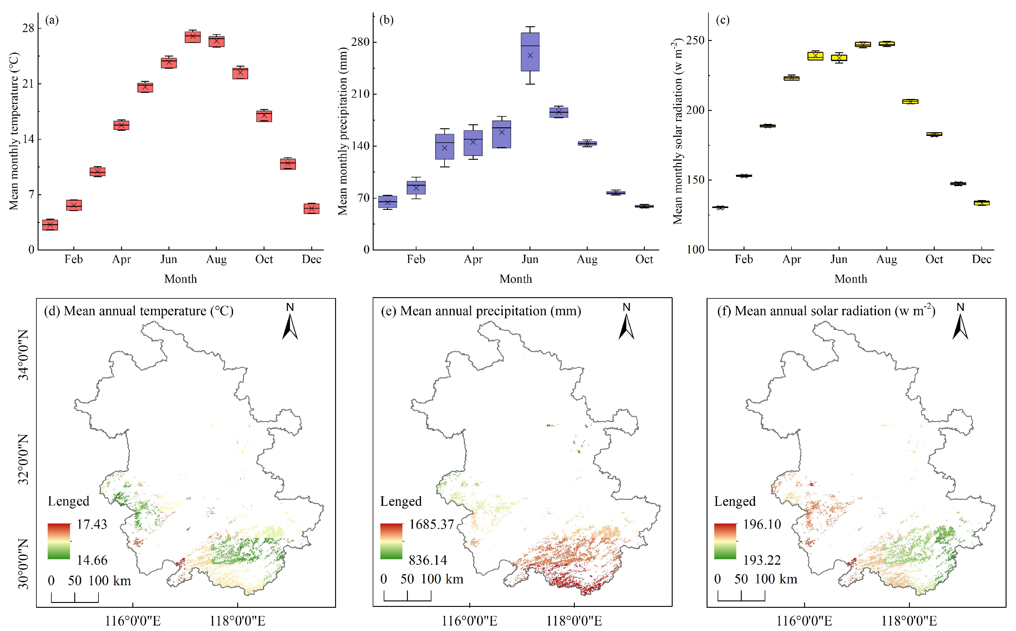
The study area is located in Anhui Province (114°54′–119°27′E, 29°41′–34°38′N), a landlocked province located in eastern China (Figure 1a). The province is characterized by a temperate monsoon climate with distinctive seasonality [28]. In this study, we focused on the forested area with no forest-type change during 2001–2020 in Anhui Province, hereafter referred as “the study area” (Figure 1b). The total area of our study area is approximately 8363 km2, with a mean annual temperature range of 14.66–17.43 °C, a mean annual cumulative precipitation range of 836.14–1685.37 mm, and a mean annual solar radiation range of 193.22–196.10 w m−2 (Figure 2d–f). Figure 2 describes the seasonal dynamics (Figure 2a–c) and the spatial distribution (Figure 2d–f) of climatic variables. Temperature, precipitation, and solar radiation all reach their peaks during summertime (Figure 2a–c). The forest types found in the province include evergreen needleleaf forest (ENF, 3.21%), evergreen broadleaf forest (EBF, 1.20%), deciduous broadleaf forest (DBF, 18.76%), and mixed forest (MF, 76.84%). Forests are mainly distributed in the southern and western regions, characterized by complex terrain which will be described in more detail in Section 2.1.2.

2.1.2. Complex Terrain

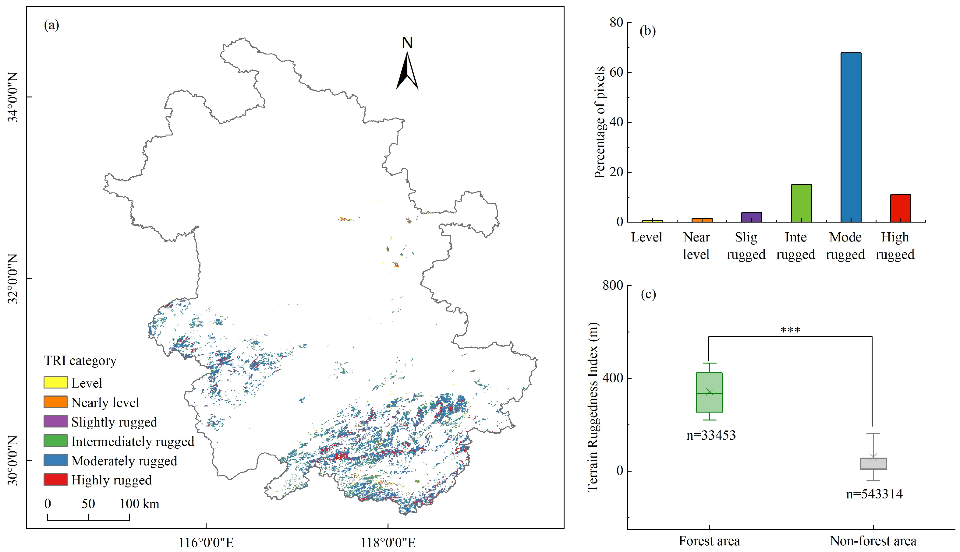
The forested area comprises numerous basins and valleys scattered around mountains, with steep elevation differences of over 1000 m. The Terrain Ruggedness Index (TRI) was used to quantify the terrain heterogeneity in the study area. The TRI highlights the amount of elevation difference between adjacent pixels and measures the square root of the averaged sum of squared elevation difference between a pixel and eight neighboring pixels for each pixel [29]. A detailed description of the digital elevation model (DEM) can be found in Section 2.2.3. Based on the TRI value, the terrain can be divided into 6 categories: level (0–80 m), nearly level (81–116 m), slightly rugged (117–161 m), intermediately rugged (162–239 m), moderately rugged (240–497 m), and highly rugged (498–958 m) [29]. Over 94% of the forest areas are intermediately rugged to highly rugged (Figure 3a,b), and the TRI in forest areas (342.71 ± 123.10 m) is significantly higher than that in non-forest areas (60.76 ± 102.30 m) (p < 0.001, Figure 3c). The aforementioned factors make this region ideal for investigating the divergent forest responses to climate fluctuations in complex terrain within close proximity.

2.2. Data Preparation

2.2.1. Satellite Data

In this study, the Enhanced Vegetation Index (EVI) was used to indicate forest responses to climate factors. Compared to the conventional Normalized Difference Vegetation Index (NDVI), the EVI is more sensitive to quantifying vegetation greenness in areas with dense vegetation, adding a blue band to the near-infrared and red bands to further enhance the vegetation signal [22]. MODIS-EVI (MOD13A3, Version 6) during 2001–2020 with a spatial resolution of 500 m and a temporal resolution of 16 days was used in this study. The average of EVI maximums in July and August was calculated to represent forest growth for each growing season [20,25,30].
The forest distribution map (Figure 1b) was derived from MODIS land cover product (MCD12Q1) during 2001–2020 with a spatial resolution of 500 m and IGBP (International Geosphere-Biosphere Programme) classification scheme [31]. Only pixels that consistently belonged to the same forest type during 2001–2020 were included in the analysis to minimize the confounding effect of land cover change on the EVI [6,7]. MODIS products could provide continuous time series of both vegetation index and land cover data for this study, so we used their spatial resolution (500 m) for data analyses instead of a higher one (e.g., Landsat image, 30 m).

2.2.2. Climate Data

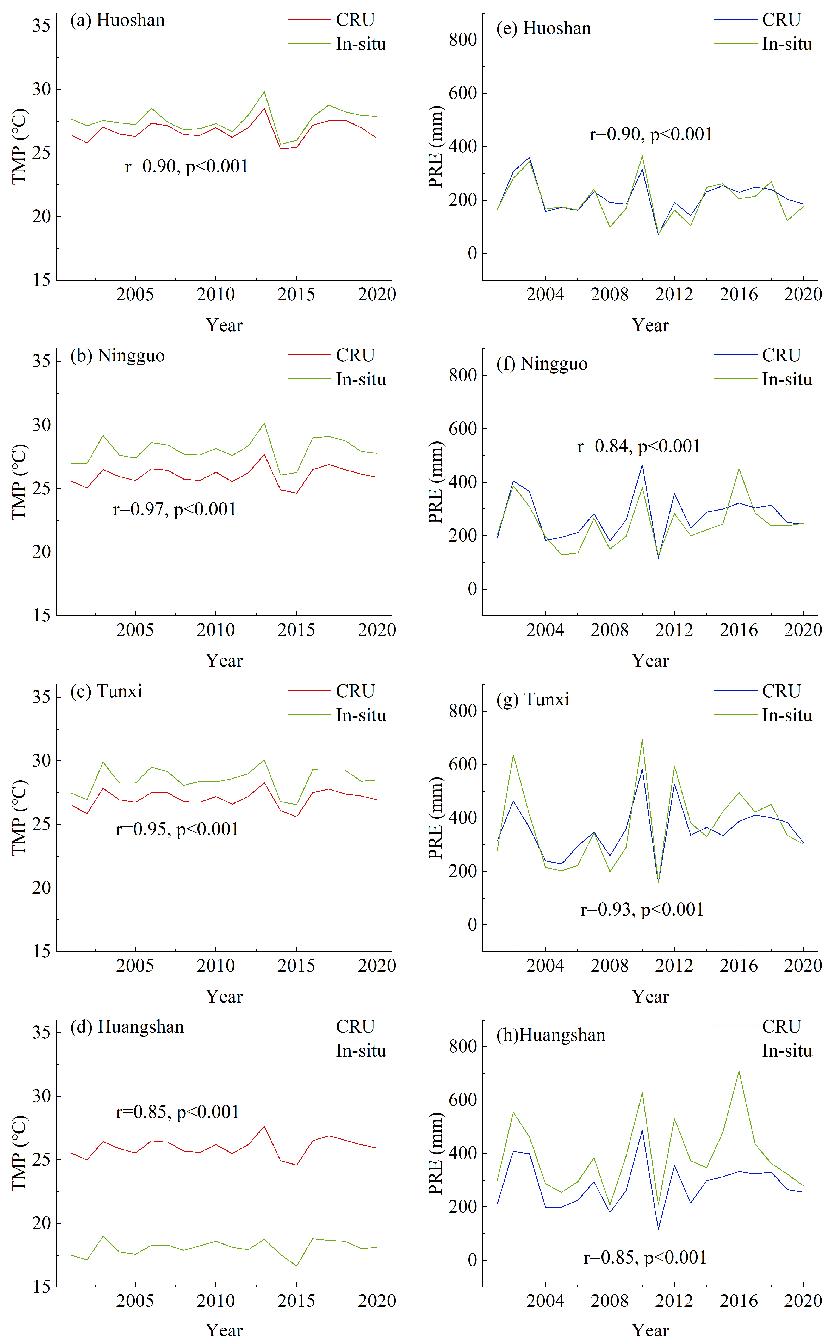
Temperature and precipitation data (2001–2020) were downloaded from the Climate Research Unit (CRU) of the University of East Anglia version TS4.06 (https://www.uea.ac.uk/groups-and-centres/climatic-research-unit, accessed on 5 March 2021), which had a monthly temporal resolution and a spatial resolution of 0.5°. The CRU dataset was one of the most commonly used climate datasets at regional scales [32,33], which was obtained via a combination of in situ meteorological station observations with anomy processing, and modeling interpolation of angular distance weighting [34]. It was well correlated with meteorological station data from China Meteorological Data Network (https://data.cma.cn/, accessed on 30 May 2022) in Anhui Province (correlation coefficients of 0.85–0.97 for temperature and 0.84–0.93 for precipitation, Figure 4). The in situ temperature data from the meteorological stations also were consistently lower than the CRU data (from the 0.5 degree grid where the stations were located), especially in the Huangshan station (Figure 4d). This is because all stations were located at their local peaks. The Huangshan station is located at the top of the Huangshan mountain 1800 m above sea level, which is much higher than the average elevation of 0.5 degree grid where the station was located. The solar radiation data (2001–2016) was downloaded from the CRU-NCEP (Climate Research Unit-National Centre for Environmental Prediction) version 7 dataset (https://rda.ucar.edu/datasets/ds314.3/, accessed on 9 May 2022), which was obtained and reprocessed from the CRU TS3.2 climate dataset and NCEP reanalysis [35]. It had a temporal resolution of 6 h, a spatial resolution of 0.5°, and the monthly average was derived for data analysis.

2.2.3. The Digital Elevation Model

The digital elevation model (DEM) used in this study was derived from the NASA Shuttle Radar Topography Mission (SRTM) data of the US Space Shuttle Endeavour with a 90 m resolution (https://srtm.csi.cgiar.org/, accessed on 12 June 2022). Based on DEM data, we calculated slope and aspect to analyze the effects of terrain on forest growth. In addition, a topographic roughness index (TRI) was calculated to quantify the terrain heterogeneity in the study area. All spatial data were reprojected with the WGS-84 geographic coordinate system and resampled to 500 m spatial resolution with the nearest neighbor algorithm. All satellite image processing was conducted in Envi5.3 (L3Harris Geospatial, Melbourne, FL, USA). All statistical analyses were con-ducted in R4.1.2 and Origin2022. All figures were created with Origin2022 (OriginLab, Northampton, MA, USA) and ArcGIS10.8 (ESRI, Redlands, CA, USA).

2.3. Research Methods

2.3.1. Identifying Time Lags of Forest Response to Different Climate Factors

It is already known that temperature, precipitation, and solar radiation can affect forest growth [5,36]. However, there are time lags between climate fluctuations and forest growth change, which can be identified with the Pearson correlation analysis [37]. For each pixel, forest growth of each growing season between 2001–2020 was indicated with the average EVI of July and August (EVIJul–Aug). Monthly average temperature (°C, 2001–2020), monthly accumulative precipitation (mm, 2001–2020), and monthly average incident solar radiation (w m−2, 2001–2016) for the same growing season has been calculated for different time windows relative to the peak growing season of July and August: Same time window (July and August), 1-month prior (June and July), 2-month prior (May and June), 3-month prior (April and May), 4-month prior (March and April), and 5-month prior (February and March) [28]. For each pixel, Pearson correlation coefficients (r) were calculated between the EVIJul–Aug of the year and each of three climate factors (TEM, PRE, and SWD) for each of six time windows (same, 1-month, 2-month, 3-month, 4-month, and 5-month prior). Correlation coefficients (r) between the EVIJul–Aug and three climate variables during six different time windows were averaged across all forested pixels in the study area where the EVI and climate factors are significantly correlated (p < 0.05). For each climate factor, the time window with the highest correlation coefficient would be chosen as the time lag of that climate factor for the following analyses.

2.3.2. Identifying the Dominating Climatic Driver for Forest Growth for Each Pixel

The relative influence of temperature, precipitation, and solar radiation on forest growth may change drastically across complex terrain within close vicinity [38,39]. For each pixel, we calculated three correlation coefficients between the EVIJul–Aug and each of three climate factors (TEM, PRE, and SWD) of their chosen optimal time windows (determined in Section 2.3.1) over 20 years. The climate factor with the maximum absolute r value with statistical significance (p < 0.05) would be considered the dominating climate diver for the pixel. According to the dominant factor in each pixel, the study area was divided into three regions: predominantly temperature-driving, precipitation-driving, and solar radiation-driving regions. These three regions were from close vicinity but with different dominant climatic drivers, which may respond to climate fluctuations differently.

2.3.3. EVI Responses to Different Climate Factors

To analyze divergent forest responses to climate fluctuations, we contrasted the EVI response to different climate conditions in predominantly temperature-driving (TMP-driving), precipitation-driving (PRE-driving), and solar radiation-driving (SWD-driving) regions. In each region, the 30-year (1991–2020) average of mean temperature during optimal time windows ( T ¯ Opt ) and its standard deviation (TSD) were calculated to represent the long-term average and its fluctuation [40]. Out of 2001–2020, the years with the maximum TOpt, the minimum TOpt, and the TOpt closest to the 30-year average T ¯ Opt were selected to be the “hot” year, the “cold” year, and the “normal” year for the region, respectively. In the “hot” year, only pixels that had TOpt higher than average TOpt of the year and the region were included for data analysis. In the “cold” year, only pixels that had TOpt lower than average TOpt of the year and the region were included for data analysis. In the “normal” year, only pixels that had TOpt within the range of 30-year average T ¯ Opt ± 1 TSD were included for data analysis. Additionally, for each region, two pair-wise t-tests were conducted among matched pixels; one to contrast hot vs. normal conditions, and one to contrast cold vs. normal conditions, in order to determine divergent forest responses to temperature change among climate-driving regions.
Similarly to temperature, the “wet” and “dry” years were chosen based on precipitation. In each region, the 30-year (1991–2020) average of accumulative precipitation during optimal time windows ( P ¯ Opt ), and its standard deviation (PSD) were calculated to represent the long-term average and its fluctuation. Out of 2001–2020, the years with the maximum POpt, the minimum POpt, and the POpt closest to the 30-year average P ¯ Opt were selected to be the “wet” year, the “dry” year and the “normal” year for the region. In the “wet” year, only pixels that had POpt higher than the average POpt of the year and the region were included for data analysis. In the “dry” year, only pixels that had POpt lower the than average POpt of the year and the region were included for data analysis. In the “normal” year, only pixels that had POpt within the range of 30-year average P ¯ Opt ± 1 PSD were included for data analysis. Additionally, for each region, two pair-wise t-tests were conducted among matched pixels; one to contrast wet vs. normal conditions, and one to contrast dry vs. normal conditions, in order to determine divergent forest responses to precipitation changes among our regions.
When we looked for the years with the maximum and minimum solar radiation ROpt using SWD data (“bright” vs. “dim” year), it was found that they coincided with the PRE data (Figure S1): the “bright” year is also the “dry” year (2011), and the dimmest years (i.e., 2002–2003 and 2010) were also the wettest years. The pixel-level correlation between POpt and ROpt during 2001–2016 was −0.822 ± 0.034 (n = 33,453 for all forested pixels). Given such a strong negative correlation between accumulative precipitation and total incident solar radiation, our analyses afterwards only focused on temperature and precipitation.

2.3.4. Partitioning the Effects of Climatic and Topographic Variables on the EVI

To quantitatively assess the effects of climate and terrain on forest growth, we used the random forest (RF) model to analyze the importance of temperature, precipitation, elevation, slope, aspect, and forest type to the EVI. RF is a classification tree-based machine-learning algorithm that is widely used in geography and ecology [41,42,43]. The %IncMSE (percentage increase in Mean Squared Error) is a metric used in random forest regression modeling to assess the importance of each independent variable. The %IncMSE is computed by randomly permuting each variable and measuring the resulting increase in mean square error (MSE) of the model predictions [43,44]. A higher %IncMSE value for a variable indicates that permuting that variable results in a larger increase in MSE, which suggests that the variable is more important for explaining forest growth in the out-of-bag cross-validation process [43,44].
Upon building the random forest model, a post hoc partial correlation analysis on elevation and slope with the EVI was conducted to further partition the impact of these two terrain variables on forest responses to climate fluctuations (i.e., r of the EVI and three climate factors calculated in Section 2.3.2). We matched the elevation data and slope data with the correlation coefficients of the EVI and climate data pixel by pixel, and then calculated the Partial correlation coefficient (R) between either elevation or slope and the Pearson correlation coefficient (r) between the EVI and climate factors. Partial correlation coefficients ρXY.Z were used to analyze the correlation between elevation (X) and the correlation coefficients (Y) between the EVI and three climate factors, in control the effect of slope (Z), hereafter referred to as ρelevation; or the impact of slope (X) on the correlation coefficients (Y) between the EVI and three climate factors, in control the effect of elevation (Z), hereafter referred to as ρslope.
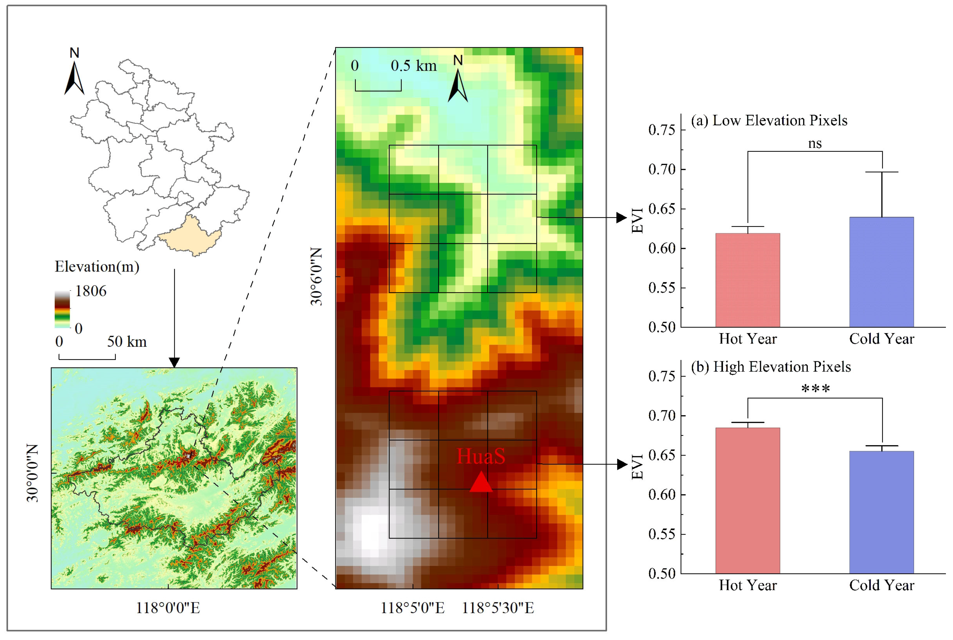
We also compared the EVI at the top and the foot of the Huangshan Mountain within close vicinity (about 1000 m apart), and for each we sampled a continuous 3 pixel × 3 pixel window. The Huangshan meteorological station is located at the top of the mountain with forest cover and has the highest elevation in the study region. We compared the EVI differences between a hot year and a cold year for both hill top and hill foot sampling areas.

3. Results

3.1. Time-Lag Effects of the EVI Response to Climate Factors

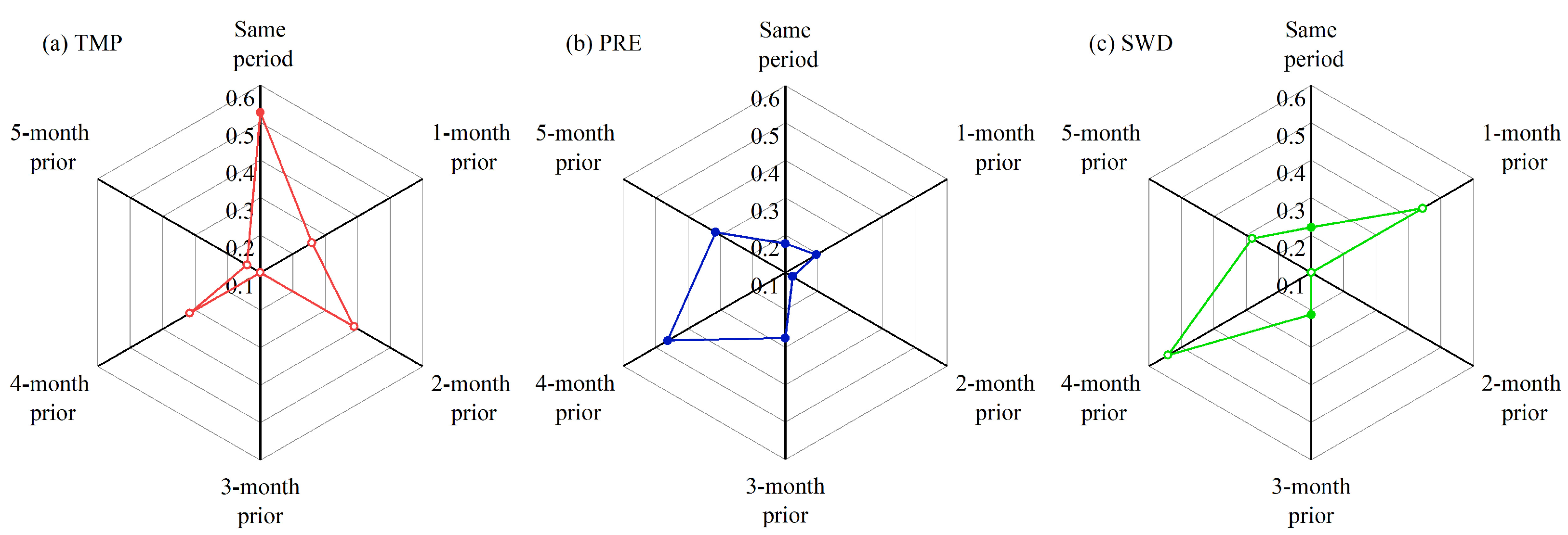
Correlation coefficient (r) between the EVIJul–Aug and temperature, precipitation, and solar radiation data within six time windows (same, 1-month, 2-month, 3-month, 4-month, and 5-month prior to July and August) are shown in Figure 5. The average EVI of July and August had the highest absolute spatial average r, with temperature in the same period (r = 0.53, indicating no time lag), with precipitation and solar radiation in 4-month prior (r = 0.46 for precipitation, r = −0.54 for solar radiation, indicating 4-month time lag). This means that forest growth in July and August had the strongest positive correlation with mean temperature in July and August, and had the strongest positive or negative correlation with accumulative precipitation or mean solar radiation in March and April, respectively. Furthermore, these results also enabled us to identify the most dominating climatic factor for each pixel.

3.2. Dominant Climate Factors Driver of the EVI

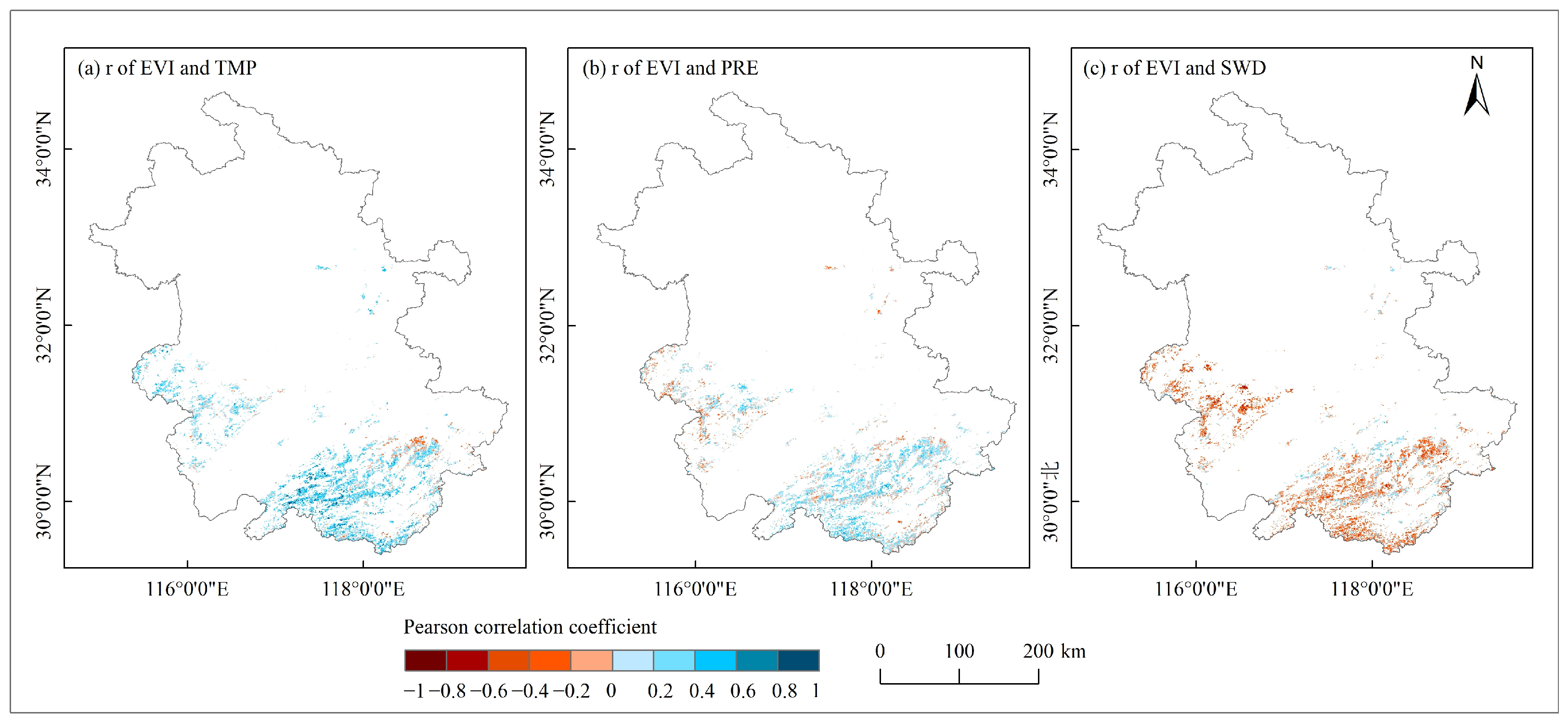
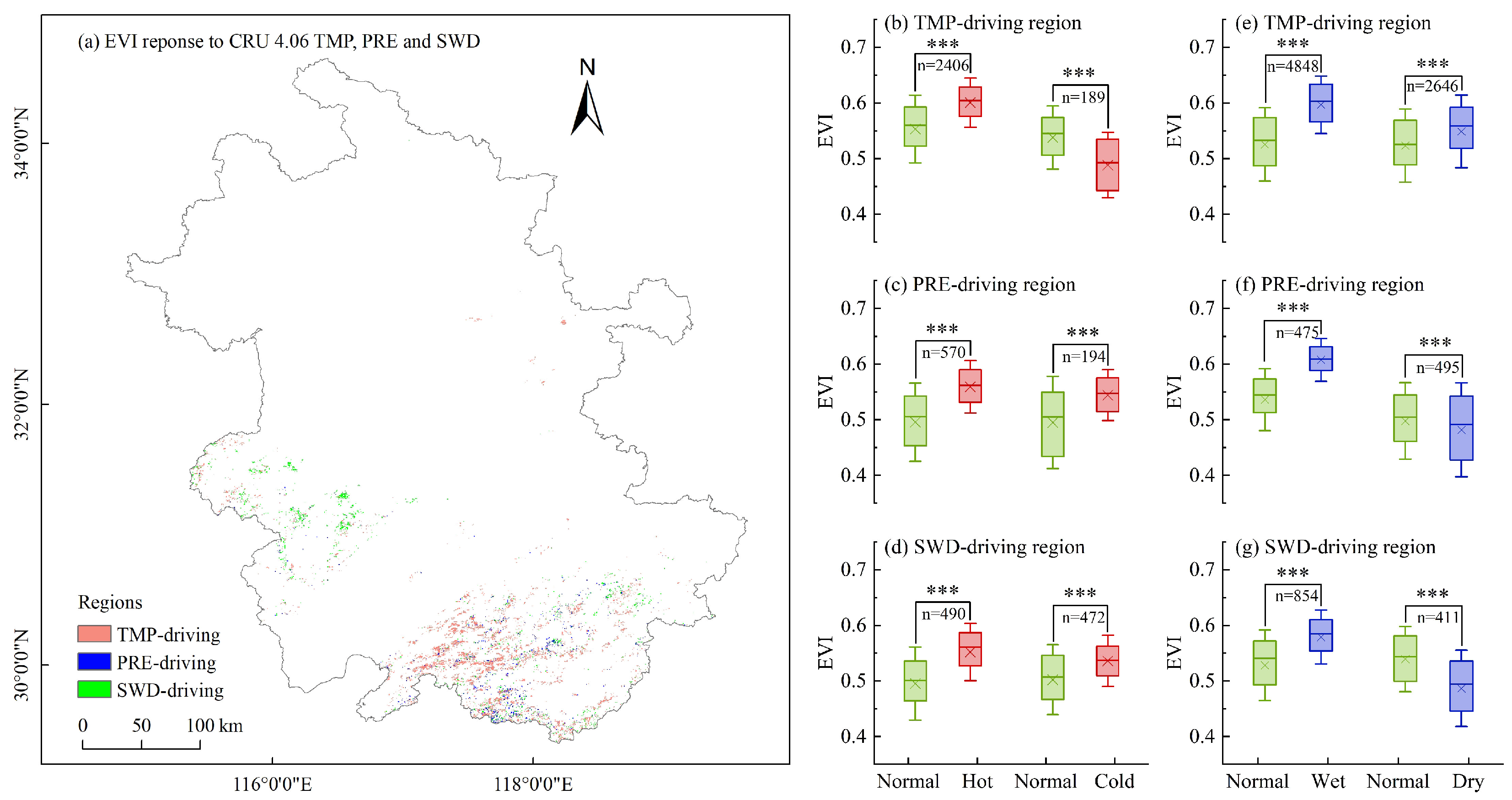
The impact of different climate factors on forest growth was not always equivalent, and there might be one dominating climatic driver which affects forest growth most strongly. We compared three correlation coefficients between the EVIJul–Aug and the climate factors of their chosen optimal time windows from Section 3.1 in each forest pixel (Figure 6). The climate factor with the maximum absolute r value with statistical significance (p < 0.05) had the strongest relationship with the EVI among the three climate factors, and was chosen as the dominating climatic driver for the pixel. Based on the correlation analyses between the EVI and climate factors, about 88.11% of the study area had a positive correlation with temperature with 18.74% being statistically significant (p < 0.05), and 11.89% showed a negative correlation with 0.19% being statistically significant (p < 0.05); 74.51% of the study area had a positive correlation with precipitation with 4.87% being statistically significant (p < 0.05), and 25.49% showed a negative correlation with 0.25% being statistically significant (p < 0.05); 28.66% of the study area had a positive correlation with solar radiation with 0.20% being statistically significant (p < 0.05), and 71.34% showed a negative correlation with 5.70% being statistically significant (p < 0.05) (Figure 6). These results suggested that temperature and precipitation promote forest growth in most areas, while radiation limits forest growth. The spatial distribution of the dominating climatic driver in the study area is shown in Figure 7a, it can be seen that the relative influence of temperature, precipitation and solar radiation on forest growth changed drastically from pixel to pixels, despite them being in close vicinity. Among the climate factors, 69% of the forest pixels EVI had the strongest correlation with temperature, and the maximum correlation coefficient of 0.86; 11% of the forest pixels EVI had the strongest correlation with precipitation, and a maximum correlation coefficient of 0.77; 20% of the forest pixels EVI had the strongest correlation with radiation, and a maximum correlation coefficient was −0.88. These results suggest that temperature, precipitation, and radiation can affect forest growth significantly in east China; however, the dominant climatic drivers vary from region to region.

3.3. Impact of Climate Fluctuations on the EVI

In the hot year (2013), pixels with TJul–Aug > 28.52 °C in the TMP-driving region, TJul–Aug > 28.36 °C in the PRE-driving region, TJul–Aug > 28.65 °C in the SWD-driving region were selected for data analysis. For the cold year (2015), the pixels with TJul–Aug < 25.47 °C in the TMP-driving region, TJul–Aug < 25.35 °C in the PRE-driving region, TJul–Aug < 25.63 °C in the SWD-driving region were selected. For the normal year (2011), the pixels with TJul–Aug ∈ 26.71 ± 0.83 °C in the TMP-driving region, TJul–Aug ∈ 26.59 ± 0.83 °C in the PRE-driving region, TJul–Aug ∈ 26.77 ± 0.84 °C in the SWD-driving region were selected. Then, for each region, two pair-wise t-tests were conducted among matched pixels, one to contrast hot vs. normal conditions (n = 2406 for the TEM region, n = 570 for the PRE region, n = 490 for the SWD region), and one to contrast cold vs. normal conditions (n = 189 for the TEM region, n = 194 for the PRE region, n = 472 for the SWD region), to reveal divergent forest responses to temperature change among the climate-driving regions. The pixels in wet, dry and normal years were selected in the same way based on Tables S1 and S2. Then, for each region, two pair-wise t-tests were used to contrast wet vs. normal conditions (n = 4848 for the TEM region, n = 475 for the PRE region, n = 854 for the SWD region) and dry vs. normal conditions (n = 2646 for the TEM region, n = 495 for the PRE region, n = 411 for the SWD region), to reveal divergent forest responses to precipitation changes among the regions.
The results of our t-test showed the EVI response to temperature and precipitation changes in Figure 7b–g: (1) In the TMP-driving region (Figure 7b), the EVI in the hot year was significantly greater than in the normal year, while significantly lower than the normal year in the cold year. This means that the EVI increased with the increase in temperature and decreased with a decrease in temperature. This result implies that warming temperatures may promote forest growth and cooling temperatures may interfere with forest growth in the TMP-driving regions. However, both the EVI in the hot and cold years were significantly greater than the normal year in Figure 7c,d. This means that temperature change (warming or cooling) may not affect the EVI in the PRE-driving region and the SWD-driving regions. (2) In the TMP-driving region (Figure 7e), the EVI in the wet and dry years was significantly greater than in the normal year. This means that precipitation change (wetness or drying) may not affect the EVI. However, both the EVI in the wet year was significantly greater than the normal year in the PRE-driving region and the SWD-driving region, while significantly lower than the normal year in the dry year (Figure 7f–g). This means that the EVI increased with an increase in precipitation and reduced with a decrease in precipitation. This result implies that increased precipitation may promote forest growth whereas decreased precipitation could interfere with forest growth in the PRE-driving region and the SWD-driving region.
A further graphic analysis on how the EVI responded to temperature and precipitation changes in different forest types (Figure S2) also shows that there were minimal differences among the forest types. These results suggested that there are significant differences in the response of forest growth to climate fluctuations (temperature, precipitation) within different regions, and such differences are related to the dominant climate factors affecting forest growth.

3.4. Impact of Elevation on Forest Response to Climate Fluctuations

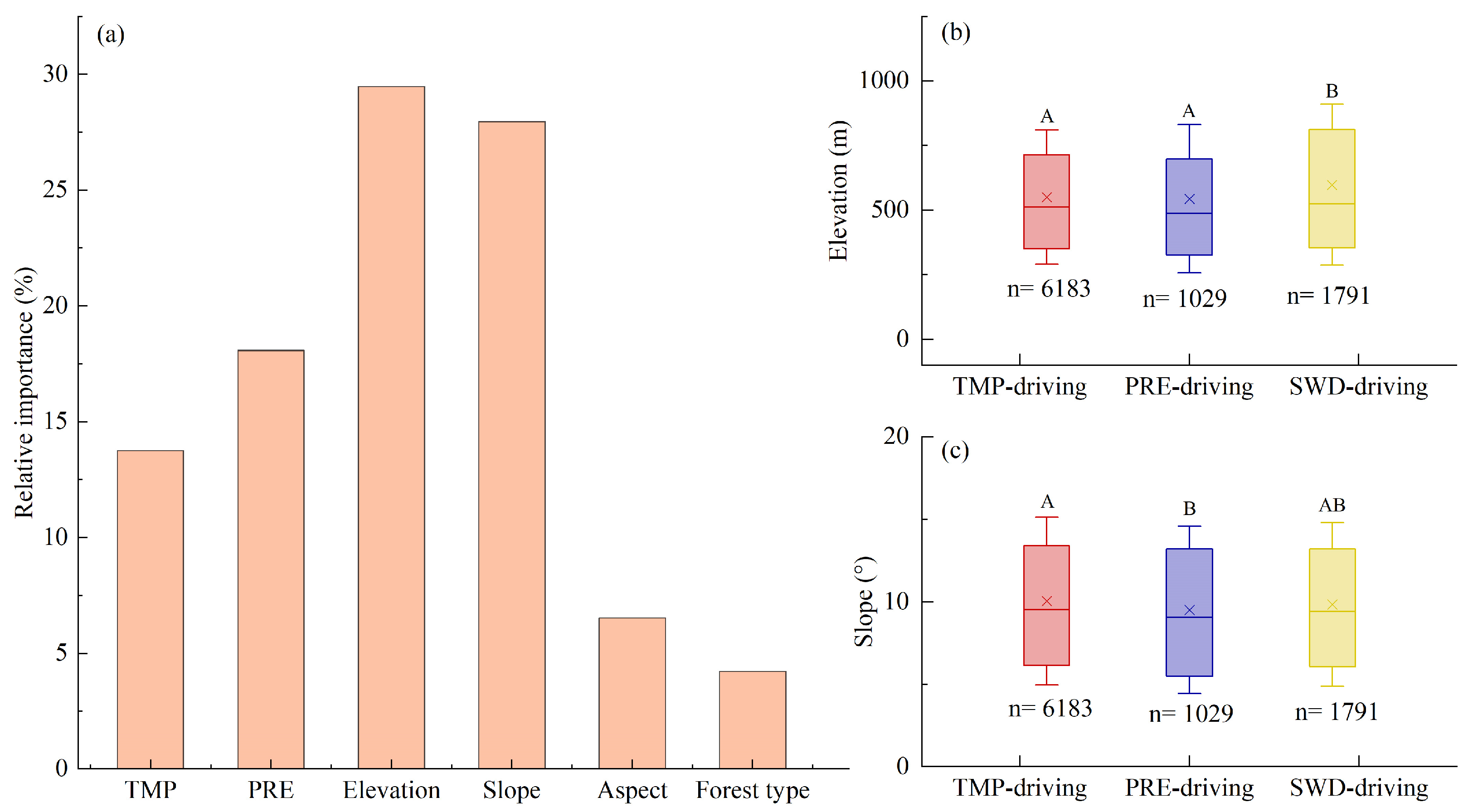
We used a random forest model to analyze the effects of temperature, precipitation, elevation, slope, aspect, and forest type on the EVI from 2001 to 2020. A total of 669,060 data points (33,453 pixels per year × 20 years) were entered into the random forest model. The importance of the six independent variables for the EVI were listed below in a descending order: elevation (29.47%) > slope (27.96%) > precipitation (18.08%) > temperature (13.75%) > aspect (6.52%) > forest type (4.21%) (Figure 8a). Due to elevation and slope being the most important factors, we further analyzed the differences in elevation and slope among three regions dominated by different climatic variables. The results showed that the elevation in the SWD-driving region was significantly higher than in TMP-driving and PRE-driving regions (Figure 8b), while the slope in the TMP-driving region was significantly higher than the PRE-driving region (Figure 8c).
Elevation had a significant positive correlation with the r of the EVI and temperature (ρelevation = 0.06, p < 0.001) in the TMP-driving region, a negative correlation with the r of the EVI and precipitation ρelevation = −0.16, p < 0.001) in the PRE-driving region, and a negative correlation with the r of the EVI and solar radiation (ρelevation = −0.07, p < 0.01) in the SWD-driving region. Slope only had a significant positive correlation with the r of the EVI and temperature (ρslope = 0.03, p < 0.05) in the TMP-driving region, but not in the other two regions. As the EVI had positive correlations with temperature and precipitation, and a negative correlation with solar radiation (Section 3.2, Figure 6a–c); therefore, these results suggest that higher elevation was associated with a stronger positive correlation of the EVI and temperature, a weaker positive correlation of the EVI with precipitation, and a stronger negative correlation of the EVI with solar radiation.
The Huangshan meteorological station is located at the top of the mountain, where forest growth was dominated by temperature (Figure 7). We compared the EVI at the station and the nearest piedmont in both the hot and cold years to reveal the effect of elevation. The results, which can be seen in Figure 9, at the top of the mountain EVI in the hot year (EVI = 0.69 ± 0.01) was significantly greater than the cold year (EVI = 0.65 ± 0.01) (Figure 9b), while at the nearest piedmont EVI had no statistic difference in the hot year (EVI = 0.62 ± 0.01) and the cold year (EVI = 0.64 ± 0.06) (Figure 9a). These two regions were within close vicinity, sharing similar climate conditions, but had different responses to temperature changes due to elevation differences.

4. Discussion

4.1. Diverse Forest Response to Climate Fluctuations

Forest growth and structure can be affected by several important climate factors, including temperature, precipitation, and solar radiation [5,36]. However, the effects of these factors on vegetation growth are not instantaneous, and can be subject to lag times [6,7,37]. For instance, precipitation takes time to infiltrate the soil, be absorbed by plant roots, and be transmitted through the xylem to the leaves for photosynthesis. Similarly, insufficient precipitation may not immediately impact vegetation growth, as soil water can reduce the effects of drought stress for a certain period [45]. On the other hand, temperature can affect vegetation growth by changing the activities of enzymes in leaves [46]. Our study found that the lag time of precipitation and radiation was longer than that of temperature, indicating that forest responses to temperature were faster than their responses to precipitation. This result was consistent with previous studies in China [27] and may be due to enzymes being more sensitive to changes in temperature [46]. Given the differences in the response times of climate factors, it is important to consider the time lag effect in studies of vegetation response to climate fluctuations.
At the global scale, the heterogeneity of hydrothermal conditions caused by latitude means that the climate drivers of forest growth can differ [5,6,7]. In high latitudes, where cold temperatures can restrict vegetation growth, forest growth is usually dominated by temperature and radiation [6,7]. Conversely, in arid and semi-arid areas at low-mid latitudes, vegetation growth is usually limited by insufficient precipitation [47]. However, the use of site data [48] or coarse-resolution spatial data [6] in global studies may overlook spatial heterogeneity in forest response to climate factors. Our study in a mountainous-hilly region of eastern China showed that forest growth is predominantly influenced by temperature, consistent with previous global results [6,7]. However, some areas were also dominated by precipitation and solar radiation, which may be related to the undulating terrain causing differences in hydrothermal conditions within close vicinity under similar climatic backgrounds [49,50]. In the troposphere, high-elevation regions were colder, with temperature and solar radiation being the dominant climatic drivers affecting forest growth, consistent with previous findings on cold regions in high latitudes [6,7].
The dominant climate factors in eastern China lead to divergent forest responses to climate fluctuations. Our results show that temperature changes had a significant impact on forest growth in the TMP-driving region, but less impact on forests in the PRE-driving and the SWD-driving regions. Warm temperatures could promote forest growth, while cold temperatures could inhibit forest growth. Precipitation changes had a significant impact on forest growth in the PRE-driving and the SWD-driving regions, but less impact on forests in the TMP-driving region. As the TMP-driving region is larger than the PRE-driving and the SWD-driving regions, forests in eastern China would generally benefit from a warming climate currently. However, a warmer and dryer climate in the future may also cause some forest patches to switch from TEM driven to PRE driven, which could lead to a decrease in forest growth instead of an increase, as predicted by existing climate models [51,52,53]. Our regional-scaled results will provide more guidance for climate fluctuations assessment for the region and local forest management policy formulation than the results from global-scaled studies.

4.2. Uncertainty

While the use of multiple data sources in this study ensured data independence, the differences in their spatiotemporal resolution may have introduced some uncertainty to the results. Other vegetation indexes, such as the MERIS Terrestrial Chlorophyll Index (MTCI), is also sensitive to chlorophyll content and could better reflect vegetation changes [23], which may be a potential index in our study. Although both the EVI and the MTCI might be appropriate for forest vegetation cover, the communication with the Envisat-1 satellite with the MERIS was lost in 2012, and the next satellite sensor allowing for the calculation of the MTCI (i.e., Sentinel) was first launched in 2014. Therefore, there is no continuous time series of the MTCI for the purpose of this study. In addition, the spatial resolution and temporal span of MODIS-EVI data match our land cover data. For this reason, we eventually chose to use the EVI dataset from the MODIS to indicate forest growth. Due to the limitation of available data, the period of solar radiation data was 4 years short of other data and not entirely consistent, which might increase uncertainties in the results. Specifically, the moderate changes in temperature and precipitation analyzed in this research led to divergent forest responses. However, extreme temperature or water stress such as frost, continuous low or high temperature, drought, and flood may lead to consistent declines in forest growth [51]. Additionally, other factors such as soil quality [13], nutrient [14], soil moisture [54], bark thickness [55], insect infestations [56], and forest wildfires [57] may also impact the responses of the EVI to climate fluctuations that may lead to low correlation coefficient value between the EVI and climate factors. Studies in other regions, such as the Tibetan plateau and India, showed that human activities such as land use and land cover management could also affect forest growth [58,59,60]. Due to the limited availability of relevant local data, it was challenging to account for these factors, which could have increased the uncertainty of our results.
We have used the Mann–Kendall test to evaluate the potential trend of the EVI increase in three regions from 2001 to 2020. The results showed that the EVI had no significant change trend in the TMP-driving and PRE-driving regions (p = 0.10 and 0.13, Figure S1a,b), while it had a significant increase in the SWD-driving region (p = 0.02, Figure S1c). Therefore, the EVI trend may have little impact on the results in the TMP-driving and PRE-driving regions (Figure 7b,c,e,f). The EVI in the hot year 2015 was lower than in the cold year 2013 in the SWD-driving region (Figure 7d), while the EVI in the dry year 2011 was lower than normal year 2009 and wet year 2010 (Figure 7g). These results are inconsistent with a hypothetic increasing trend of the EVI. In addition, the years we chose here were very close (2011 to 2015 for temperature, 2009 to 2011 for precipitation); therefore, the influence of a potential EVI increasing trend might be minimal given these time spans.

5. Conclusions

This study provides new insights into the divergent forest responses to temperature and precipitation changes within close vicinity, using satellite data and climate data. Our results show that warming temperature can promote forest growth, while cooling temperature can limit forest growth in the temperature-driven regions. Similarly, wet precipitation can promote forest growth while drying precipitation can limit forest growth in the precipitation-driven regions and the solar radiation-driven regions. These results showed that complex terrain contributed significantly to the spatial heterogeneity of forest response to climatic drivers at the regional scale, which has important implications for forest resource management and policy decisions. Our findings highlight the importance of considering the heterogeneity of forest responses to climate fluctuations, particularly in a future warmer and drier climate, where some forest patches may switch from temperature driven to precipitation driven, leading to restricted forest growth rather than improved forest growth as predicted by existing climate models. Therefore, it is important to incorporate these divergent forest responses in local forest management and climate change-related risk assessments.

Supplementary Materials

The following supporting information can be downloaded at: https://www.mdpi.com/article/10.3390/rs15112749/s1, Figure S1: Time series of the monthly average EVI (enhanced vegetation index, panel a–c), monthly average temperature (TMP (°C), panel d–f), monthly accumulative precipitation (PRE (mm), panel g–i), and monthly average solar radiation (SWD (w m−2), panel j–l) in regions dominated by different climate factors (panel a,d,g,j are TMP-driving; panel b,e,h,k are PRE-driving, and panel c,f,i,l are SWD-driving). Figure S2: Responses of the regional Enhanced Vegetation Index (EVI) to temperature and precipitation changes mainly driven by temperature (TMP), precipitation (PRE) and solar radiation (SWD) within each forest type (ENF: evergreen needle-leafed forest; EBF: evergreen broad-leafed forest; DBF: deciduous broad-leafed forest; MF: mixed forest) in regions predominantly driven by different climate factors. Table S1: The maximum and minimum annual mean of temperature (TMP, °C), precipitation (PRE, mm), or radiation (SWD, w m−2), near 30-year average, and their corresponding years during 2001–2020 in regions driven by TMP, PRE and SWD. Table S2: The 30-year average of temperature (TMP, °C), precipitation (PRE, mm), or radiation (SWD, w m−2), and their standard deviation in regions driven by TMP, PRE and SWD.

Author Contributions

Conceptualization, P.X. and W.F.; data curation, J.W.; funding acquisition, P.X.; methodology, P.X. and W.F.; project administration, P.X.; resources, W.F.; visualization, J.W.; writing—original draft, J.W.; writing—review and editing, H.L., D.C., Z.W., Y.Y. and C.R. All authors have read and agreed to the published version of the manuscript.

Funding

This research was funded by the National Natural Science Foundation of China (grant no. 42001348), the Key Research and Development Program of Anhui Province (grant no. 2022107020028; 2021003), and the Natural Science Foundation of Anhui Province of China (grant no. 2008085QD167). D.C. was funded by the Major Science and Technology Project of High-Resolution Earth Observation System (grant no. 76Y50G14-0038-22/23), the Anhui Provincial Special Support Plan (2019), and the Research Project of Anhui Provincial College Excellent Youth (grant no. 2022AH020069). H.L. was funded by the Science and Technology Major Project of Anhui Province of China (grant no. 202003a06020002). Z.W. was funded by the Key Project of Anhui Provincial College Excellent Youth Talents Support Program in 2022 (grant no. 13).

Data Availability Statement

All data or code generated or used during this study are available from the author by request ([email protected]).

Acknowledgments

We thank the six anonymous reviewers for their constructive and insightful comments and suggestions which helped us to improve this manuscript in all aspects.

Conflicts of Interest

The authors declare no conflict of interest.

References

  1. Dixon, R.K.; Solomon, A.M.; Brown, S.; Houghton, R.A.; Trexier, M.C.; Wisniewski, J. Carbon Pools and Flux of Global Forest Ecosystems. Science 1994, 263, 185–190. [Google Scholar] [CrossRef]
  2. Bonan, G.B. Forests and Climate Change: Forcings, Feedbacks, and the Climate Benefits of Forests. Science 2008, 320, 1444–1449. [Google Scholar] [CrossRef] [PubMed]
  3. Baldocchi, D.; Chu, H.; Reichstein, M. Inter-Annual Variability of Net and Gross Ecosystem Carbon Fluxes: A Review. Agric. For. Meteorol. 2018, 249, 520–533. [Google Scholar] [CrossRef]
  4. Seppälä, R.; Buck, A.; Katila, P. Adaptation of Forests and People to Climate Change; International Union of Forest Research Organizations (IUFRO): Helsinki, Finland, 2009; Volume 22, p. 224. [Google Scholar]
  5. Nemani, R.R.; Keeling, C.D.; Hashimoto, H.; Jolly, W.M.; Piper, S.C.; Tucker, C.J.; Myneni, R.B.; Running, S.W. Climate-Driven Increases in Global Terrestrial Net Primary Production from 1982 to 1999. Science 2003, 300, 1560–1563. [Google Scholar] [CrossRef] [PubMed]
  6. Wu, D.; Zhao, X.; Liang, S.; Zhou, T.; Huang, K.; Tang, B.; Zhao, W. Time-Lag Effects of Global Vegetation Responses to Climate Change. Glob. Chang. Biol. 2015, 21, 3520–3531. [Google Scholar] [CrossRef]
  7. Ding, Y.; Li, Z.; Peng, S. Global Analysis of Time-Lag and -Accumulation Effects of Climate on Vegetation Growth. Int. J. Appl. Earth Obs. Geoinf. 2020, 92, 102179. [Google Scholar] [CrossRef]
  8. Allen, C.D.; Breshears, D.D.; McDowell, N.G. On Underestimation of Global Vulnerability to Tree Mortality and Forest Die-off from Hotter Drought in the Anthropocene. Ecosphere 2015, 6, 129. [Google Scholar] [CrossRef]
  9. Franke, A.K.; Bräuning, A.; Timonen, M.; Rautio, P. Growth Response of Scots Pines in Polar-Alpine Tree-Line to a Warming Climate. For. Ecol. Manag. 2017, 399, 94–107. [Google Scholar] [CrossRef]
  10. Allen, C.D.; Macalady, A.K.; Chenchouni, H.; Bachelet, D.; McDowell, N.; Vennetier, M.; Kitzberger, T.; Rigling, A.; Breshears, D.D.; Hogg, E.H.; et al. A Global Overview of Drought and Heat-Induced Tree Mortality Reveals Emerging Climate Change Risks for Forests. For. Ecol. Manag. 2010, 259, 660–684. [Google Scholar] [CrossRef]
  11. Krasnova, A.; Mander, U.; Noe, S.M.; Uri, V.; Krasnov, D.; Soosaar, K. Hemiboreal Forests? CO2 Fluxes Response to the European 2018 Heatwave. Agric. For. Meteorol. 2022, 323, 109042. [Google Scholar] [CrossRef]
  12. Xiong, Y.; Li, Y.; Xiong, S.; Wu, G.; Deng, O. Multi-Scale Spatial Correlation between Vegetation Index and Terrain Attributes in a Small Watershed of the Upper Minjiang River. Ecol. Indic. 2021, 126, 107610. [Google Scholar] [CrossRef]
  13. Teng, H.; Chen, S.; Hu, B.; Shi, Z. Future Changes and Driving Factors of Global Peak Vegetation Growth Based on CMIP6 Simulations. Ecol. Inform. 2023, 75, 102031. [Google Scholar] [CrossRef]
  14. Viana Cunha, H.F.; Andersen, K.M.; Lugli, L.F.; Santana, F.D.; Aleixo, I.F.; Moraes, A.M.; Garcia, S.; Di Ponzio, R.; Mendoza, E.O.; Brum, B.; et al. Direct Evidence for Phosphorus Limitation on Amazon Forest Productivity. Nature 2022, 608, 558–562. [Google Scholar] [CrossRef]
  15. Tucker, C.J. Red and Photographic Infrared Linear Combinations for Monitoring Vegetation. Remote Sens. Environ. 1979, 8, 127–150. [Google Scholar] [CrossRef]
  16. Deshayes, M.; Guyon, D.; Jeanjean, H.; Stach, N.; Jolly, A.; Hagolle, O. The Contribution of Remote Sensing to the Assessment of Drought Effects in Forest Ecosystems. Ann. For. Sci. 2006, 63, 579–595. [Google Scholar] [CrossRef]
  17. Assal, T.J.; Anderson, P.J.; Sibold, J. Spatial and Temporal Trends of Drought Effects in a Heterogeneous Semi-Arid Forest Ecosystem. For. Ecol. Manag. 2016, 365, 137–151. [Google Scholar] [CrossRef]
  18. Xu, P.; Fang, W.; Zhou, T.; Zhao, X.; Luo, H.; Hendrey, G.; Yi, C. Spatial Upscaling of Tree-Ring-Based Forest Response to Drought with Satellite Data. Remote Sens. 2019, 11, 2344. [Google Scholar] [CrossRef]
  19. Dorman, M.; Svoray, T.; Perevolotsky, A.; Sarris, D. Forest Performance during Two Consecutive Drought Periods: Diverging Long-Term Trends and Short-Term Responses along a Climatic Gradient. For. Ecol. Manag. 2013, 310, 1–9. [Google Scholar] [CrossRef]
  20. Xu, P.; Zhou, T.; Zhao, X.; Luo, H.; Gao, S.; Li, Z.; Cao, L. Diverse Responses of Different Structured Forest to Drought in Southwest China through Remotely Sensed Data. Int. J. Appl. Earth Obs. Geoinf. 2018, 69, 217–225. [Google Scholar] [CrossRef]
  21. Song, L.; Li, Y.; Ren, Y.; Wu, X.; Guo, B.; Tang, X.; Shi, W.; Ma, M.; Han, X.; Zhao, L. Divergent Vegetation Responses to Extreme Spring and Summer Droughts in Southwestern China. Agric. For. Meteorol. 2019, 279, 107703. [Google Scholar] [CrossRef]
  22. Wang, Z.; Liu, C.; Huete, A. From AVHRR-NDVI to MODIS-EVI: Advances in vegetation index research. Acta Ecol. Sin. 2003, 23, 979–987. [Google Scholar] [CrossRef]
  23. Dash, J.; Curran, P.J. Evaluation of the MERIS Terrestrial Chlorophyll Index (MTCI). Adv. Space Res. 2007, 39, 100–104. [Google Scholar] [CrossRef]
  24. Xu, P.; Fang, W.; Zhou, T.; Li, H.; Zhao, X.; Berman, S.; Zhang, T.; Yi, C. Satellite Evidence of Canopy-Height Dependence of Forest Drought Resistance in Southwestern China. Environ. Res. Lett. 2022, 17, 025005. [Google Scholar] [CrossRef]
  25. Xu, P.; Zhou, T.; Yi, C.; Luo, H.; Zhao, X.; Fang, W.; Gao, S.; Liu, X. Impacts of Water Stress on Forest Recovery and Its Interaction with Canopy Height. Int. J. Environ. Res. Public Health 2018, 15, 1257. [Google Scholar] [CrossRef]
  26. Yi, C.; Jackson, N. A Review of Measuring Ecosystem Resilience to Disturbance. Environ. Res. Lett. 2021, 16, 053008. [Google Scholar] [CrossRef]
  27. Xie, H.; Tong, X.; Li, J.; Zhang, J.; Liu, P.; Yu, P. Changes of NDVI and EVI and their responses to climatic variables in the Yellow River Basin during the growing season of 2000–2018. Acta Ecol. Sin. 2022, 42, 4536–4549. [Google Scholar] [CrossRef]
  28. Xu, G.; Yang, X.; Xu, X.; Li, A.; Yang, Q. Dynamic changes of monthly NDVI in Anhui Province under climate warming. Resour. Environ. Yangtze Basin 2021, 30, 397–406. [Google Scholar]
  29. Riley, S.J.; De Gloria, S.D.; Elliot, R. Index that quantifies topographic heterogeneity. Intermount. J. Sci. 1999, 5, 23–27. [Google Scholar]
  30. Luo, H.; Zhou, T.; Wu, H.; Zhao, X.; Wang, Q.; Gao, S.; Li, Z. Contrasting Responses of Planted and Natural Forests to Drought Intensity in Yunnan, China. Remote Sens. 2016, 8, 635. [Google Scholar] [CrossRef]
  31. Loveland, T.; Zhu, Z.; Ohlen, D.; Brown, J.; Redd, B.; Yang, L. An Analysis of IGBP Global Land-Cover Characterization Process. Photogramm. Eng. Remote Sens. 1999, 65, 1069–1074. [Google Scholar]
  32. Verhoeven, E.; Wardle, G.M.; Roth, G.W.; Greenville, A.C. Characterising the Spatiotemporal Dynamics of Drought and Wet Events in Australia. Sci. Total Environ. 2022, 846, 157480. [Google Scholar] [CrossRef]
  33. Weijers, S. Declining Temperature and Increasing Moisture Sensitivity of Shrub Growth in the Low-Arctic Erect Dwarf-Shrub Tundra of Western Greenland. Ecol. Evol. 2022, 12, e9419. [Google Scholar] [CrossRef] [PubMed]
  34. Harris, I.; Osborn, T.J.; Jones, P.; Lister, D. Version 4 of the CRU TS Monthly High-Resolution Gridded Multivariate Climate Dataset. Sci. Data 2020, 7, 109. [Google Scholar] [CrossRef] [PubMed]
  35. Viovy, N. CRUNCEP Version 7–Atmospheric Forcing Data for the Community Land Model, Research Data Archive at the National Center for Atmospheric Research; Computational and Information Systems Lab: Boulder, CO, USA, 2018. [Google Scholar] [CrossRef]
  36. Wei, H.; Zhao, X.; Liang, S.; Zhou, T.; Wu, D.; Tang, B. Effects of Warming Hiatuses on Vegetation Growth in the Northern Hemisphere. Remote Sens. 2018, 10, 683. [Google Scholar] [CrossRef]
  37. Li, P.; Wang, J.; Liu, M.; Xue, Z.; Bagherzadeh, A.; Liu, M. Spatio-Temporal Variation Characteristics of NDVI and Its Response to Climate on the Loess Plateau from 1985 to 2015. Catena 2021, 203, 105331. [Google Scholar] [CrossRef]
  38. Zapata-Rios, X.; Brooks, P.D.; Troch, P.A.; McIntosh, J.; Guo, Q. Influence of Terrain Aspect on Water Partitioning, Vegetation Structure and Vegetation Greening in High-Elevation Catchments in Northern New Mexico. Ecohydrology 2016, 9, 782–795. [Google Scholar] [CrossRef]
  39. He, J.; Shi, X.; Fu, Y. Identifying Vegetation Restoration Effectiveness and Driving Factors on Different Micro-Topographic Types of Hilly Loess Plateau: From the Perspective of Ecological Resilience. J. Environ. Manag. 2021, 289, 112562. [Google Scholar] [CrossRef]
  40. Yuan, D.; Lu, E.; Dai, W.; Chao, Q.; Wang, H.; Li, S. The Ice-and-Snow Tourism in Harbin Met Its Waterloo: Analysis of the Causes of the Warm Winter with Reduced Snowfall in 2018/2019. Atmosphere 2022, 13, 1091. [Google Scholar] [CrossRef]
  41. Cutler, D.R.; Edwards, T.C.; Beard, K.H.; Cutler, A.; Hess, K.T. Random Forests for Classification in Ecology. Ecology 2007, 88, 2783–2792. [Google Scholar] [CrossRef]
  42. Wei, S.; Yi, C.; Fang, W.; Hendrey, G. A Global Study of GPP Focusing on Light-Use Efficiency in a Random Forest Regression Model. Ecosphere 2017, 8, e01724. [Google Scholar] [CrossRef]
  43. Du, X.; Zhao, X.; Zhou, T.; Jiang, B.; Xu, P.; Wu, D.; Tang, B. Effects of Climate Factors and Human Activities on the Ecosystem Water Use Efficiency throughout Northern China. Remote Sens. 2019, 11, 2766. [Google Scholar] [CrossRef]
  44. Ye, T.; Zhao, N.; Yang, X.; Ouyang, Z.; Liu, X.; Chen, Q.; Hu, K.; Yue, W.; Qi, J.; Li, Z.; et al. Improved Population Mapping for China Using Remotely Sensed and Points-of-Interest Data within a Random Forests Model. Sci. Total Environ. 2019, 658, 936–946. [Google Scholar] [CrossRef] [PubMed]
  45. Lebourgeois, F.; Rathgeber, C.B.K.; Ulrich, E. Sensitivity of French Temperate Coniferous Forests to Climate Variability and Extreme Events (Abies alba, Picea abies and Pinus sylvestris). J. Veg. Sci. 2010, 21, 364–376. [Google Scholar] [CrossRef]
  46. Moore, C.E.; Meacham-Hensold, K.; Lemonnier, P.; Slattery, R.A.; Benjamin, C.; Bernacchi, C.J.; Lawson, T.; Cavanagh, A.P. The Effect of Increasing Temperature on Crop Photosynthesis: From Enzymes to Ecosystems. J. Exp. Bot. 2021, 72, 2822–2844. [Google Scholar] [CrossRef] [PubMed]
  47. Jiang, H.; Xu, X.; Guan, M.; Wang, L.; Huang, Y.; Jiang, Y. Determining the Contributions of Climate Change and Human Activities to Vegetation Dynamics in Agro-Pastural Transitional Zone of Northern China from 2000 to 2015. Sci. Total Environ. 2020, 718, 134871. [Google Scholar] [CrossRef] [PubMed]
  48. Tejedor, E.; Serrano-Notivoli, R.; de Luis, M.; Saz, M.A.; Hartl, C.; George, S.; Buntgen, U.; Liebhold, A.M.; Vuille, M.; Esper, J. A Global Perspective on the Climate-Driven Growth Synchrony of Neighbouring Trees. Glob. Ecol. Biogeogr. 2020, 29, 1114–1125. [Google Scholar] [CrossRef]
  49. Herrmann, S.M.; Didan, K.; Barreto-Munoz, A.; Crimmins, M.A. Divergent Responses of Vegetation Cover in Southwestern US Ecosystems to Dry and Wet Years at Different Elevations. Environ. Res. Lett. 2016, 11, 124005. [Google Scholar] [CrossRef]
  50. Li, X.; Du, H.; Zhou, G.; Mao, F.; Zhu, D.; Zhang, M.; Xu, Y.; Zhou, L.; Huang, Z. Spatiotemporal Patterns of Remotely Sensed Phenology and Their Response to Climate Change and Topography in Subtropical Bamboo Forests during 2001–2017: A Case Study in Zhejiang Province, China. GIScience Remote Sens. 2023, 60, 2163575. [Google Scholar] [CrossRef]
  51. Xie, Y.; Wang, X.; Silander, J.A. Deciduous Forest Responses to Temperature, Precipitation, and Drought Imply Complex Climate Change Impacts. Proc. Natl. Acad. Sci. USA 2015, 112, 13585–13590. [Google Scholar] [CrossRef]
  52. Li, G.; Chen, W.; Zhang, X.; Bi, P.; Yang, Z.; Shi, X.; Wang, Z. Spatiotemporal Dynamics of Vegetation in China from 1981 to 2100 from the Perspective of Hydrothermal Factor Analysis. Environ. Sci. Pollut. Res. 2022, 29, 14219–14230. [Google Scholar] [CrossRef]
  53. Li, G.; Chen, W.; Mu, L.; Zhang, X.; Bi, P.; Wang, Z.; Yang, Z. Analysis and Prediction of Global Vegetation Dynamics: Past Variations and Future Perspectives. J. For. Res. 2023, 34, 317–332. [Google Scholar] [CrossRef]
  54. Du, R.; Wu, J.; Tian, F.; Yang, J.; Han, X.; Chen, M.; Zhao, B.; Lin, J. Reversal of Soil Moisture Constraint on Vegetation Growth in North China. Sci. Total Environ. 2023, 865, 161246. [Google Scholar] [CrossRef] [PubMed]
  55. McHugh, C.W.; Kolb, T.E. Ponderosa Pine Mortality Following Fire in Northern Arizona. Int. J. Wildland Fire 2003, 12, 7–22. [Google Scholar] [CrossRef]
  56. Kitchens, K.A.; Peng, L.; Daniels, L.D.; Carroll, A.L. Patterns of Infestation by Subcortical Insects (Coleoptera: Buprestidae, Cerambycidae) after Widespread Wildfires in Mature Douglas-Fir (Pseudotsuga menziesii) Forests. For. Ecol. Manag. 2022, 513, 120203. [Google Scholar] [CrossRef]
  57. Yang, J.; Zhang, Q.; Hao, S. Effects of Fire Disturbance on Larix gmelinii Growth-Climate Relationship. Ecol. Indic. 2022, 143, 109377. [Google Scholar] [CrossRef]
  58. Sarmah, S.; Jia, G.; Zhang, A. Satellite View of Seasonal Greenness Trends and Controls in South Asia. Environ. Res. Lett. 2018, 13, 034026. [Google Scholar] [CrossRef]
  59. Chen, C.; Park, T.; Wang, X.; Piao, S.; Xu, B.; Chaturvedi, R.K.; Fuchs, R.; Brovkin, V.; Ciais, P.; Fensholt, R.; et al. China and India Lead in Greening of the World through Land-Use Management. Nat. Sustain. 2019, 2, 122–129. [Google Scholar] [CrossRef]
  60. Parida, B.R.; Pandey, A.C.; Patel, N.R. Greening and Browning Trends of Vegetation in India and Their Responses to Climatic and Non-Climatic Drivers. Climate 2020, 8, 92. [Google Scholar] [CrossRef]
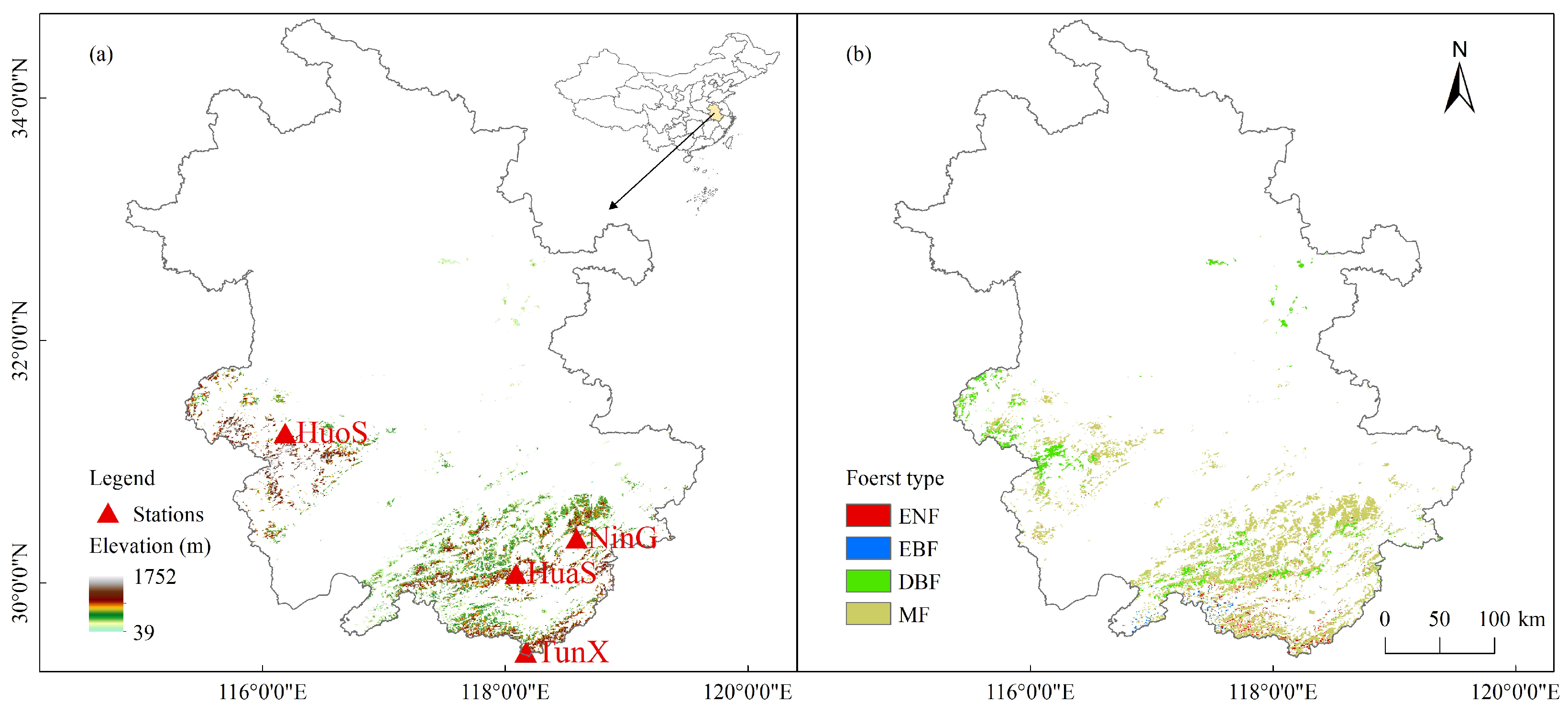
Figure 1. Distribution of elevation (a) and forest types (b) in the study area (i.e., forested pixels with no forest-type change during 2001–2020 in Anhui Province, hereafter referred as “the study area”). Panel (a): the digital elevation model (DEM, resampled to 500 m resolution) of the study area with four meteorological stations (Huoshan, Ningguo, Huangshan, and Tunxi). Panel (b): the distribution of forest types (EN: evergreen needle-leafed forest, EB: evergreen broad-leafed forest, DB: deciduous broad-leafed forest, and MF: mixed forest) in the study area (500 m resolution).
Remotesensing 15 02749 g001
Figure 2. Seasonal dynamics (panel (ac)) and spatial heterogeneity (panel (df)) of climatic variables during 2001–2020 in the study area. Panel (a): Mean monthly temperature (°C). Panel (b): Mean monthly precipitation (mm). Panel (c): Mean monthly radiation (w m−2). Panel (d): Mean annual temperature (°C). Panel (e): Mean annual precipitation (mm). Panel (f): Mean annual radiation (w m−2).
Remotesensing 15 02749 g002
Figure 3. Distribution of the Terrain Ruggedness Index (TRI) in the study area. In Panel (a,b): the six TRI categories include level (0–80 m), nearly level (81–116 m), slightly rugged (117–161 m), intermediately rugged (162–239 m), moderately rugged (240–497 m), and highly rugged (498–958 m). Panel (a): Spatial distribution of the Terrain Ruggedness Index. Panel (b): Percentage of pixels in each TRI category. Panel (c): TRI contrast between forest area (the focus of this study) and non-forest area in Anhui Province. *** indicates highly significant difference between means with p < 0.001.
Remotesensing 15 02749 g003
Figure 4. Time series of mean monthly temperatures of July and August (TMP, °C) and accumulative precipitation of March and April (PRE, mm) from in situ meteorological stations (green lines: (a,e). Huoshan station; (b,f). Ningguo station; (c,g). Tunxi station; (d,h). Huangshan station) and from reanalyzed Climate Research Unit (CRU) data (red lines for TMP; blue lines for PRE). r presents the Pearson correlation coefficient of temperature (panel (ad)) and precipitation (panel (eh)) between in situ data and CRU data for each meteorological station.
Remotesensing 15 02749 g004
Figure 5. Correlation coefficients (r) between the Enhanced Vegetation Index (EVIJul–Aug) and climate factors (panel (a) TMP: two-month mean temperature (red lines). Panel (b) PRE: two-month accumulative precipitation (blue lines). Panel (c) SWD: two-month mean solar radiation (green lines) during six different time windows (same, 1-month, 2-month, 3-month, 4-month, and 5-month prior to the two-month period of July and August), averaged across all forested pixels in the study area where the EVI and climate factors are significantly correlated.
Remotesensing 15 02749 g005
Figure 6. The Pearson correlation coefficients (r) of the Enhanced Vegetation Index (EVI) with each of the three climate factors—mean monthly temperature (TMP, (a)), accumulative precipitation (PRE, (b)), and mean monthly solar radiation (SWD, (c)) in the study area.
Remotesensing 15 02749 g006
Figure 7. The spatial distribution of forested regions predominantly driven by different climate factors (a), and their differential responses of the Enhanced Vegetation Index (EVI) to changes in temperature (bd) and precipitation (eg). In panel a, predominantly temperature-driving (TMP, red), precipitation-driving (PRE, blue), and solar radiation-driving (SWD, green) regions were determined by the climate factor that had the highest correlation coefficient with the EVI. In panel b–d, the EVI in the high-temperature year (hot, in red, year 2013) or in the low-temperature year (cold, in red, year 2015) were contrasted with the normal-temperature year (normal, in green, year 2011) in TMP-driving (b), PRE-driving (c), and SWD-driving (d) regions. In panel e–g, the EVI in the high-precipitation year (wet, in blue, year 2010) or the low-precipitation year (dry, in blue, year 2011) were contrasted with the normal-precipitation year (normal, in green, year 2009) in TMP-driving (e), PRE-driving (f), and SWD-driving (g) regions. n represents the number of pixels. *** indicates p < 0.001 for pairwise t-tests.
Remotesensing 15 02749 g007
Figure 8. The impact of terrain on forest responses to climate factors based on random forest models. Panel (a) is the relative importance of various forces on the EVI. Panel (b,c) are the boxplots of elevation (b) and slope (c) among three climate-driving regions. TMP: mean monthly temperature (°C); PRE: accumulative precipitation (mm); SWD: mean monthly downward short-wave radiation (w m−2); n represents the number of pixels. In Panel (b,c), Letter A and B indicate means were significantly different from each other (p < 0.05) with Scheffe test. Letter AB indicates mean was not significantly different from means with either A or B.
Remotesensing 15 02749 g008
Figure 9. The impact of elevation on forest responses to temperature change based on pixels in 3 × 3 window taken from adjacent areas in Huangshan station with a resolution of 500 m. The Enhanced Vegetation Index (EVI) in high-elevation pixels were significantly higher in the hot year (red bar, year 2013) than in the cold year (blue bar, year 2015) (panel (b)), while the EVI in low-elevation pixels had no difference of growth between the hot and the cold years (panel (a)). ns indicates no significant difference between means. *** indicates highly significant difference between means with p < 0.001.
Remotesensing 15 02749 g009
Disclaimer/Publisher’s Note: The statements, opinions and data contained in all publications are solely those of the individual author(s) and contributor(s) and not of MDPI and/or the editor(s). MDPI and/or the editor(s) disclaim responsibility for any injury to people or property resulting from any ideas, methods, instructions or products referred to in the content.