Confidence Intervals and Regions for Proportions under Various Three-Endmember Linear Mixture Models

Abstract

Many studies in recent years have been devoted to estimating the per-pixel proportions of three broad classes of materials (e.g., photosynthetic vegetation, non-photosynthetic vegetation and bare soil) using data from multispectral sensors. Oftentimes, the estimated proportions are used to monitor environmental change in both urban and non-urban environments. Many of these papers use proportion estimation methods based on the linear mixture model. Very few of these papers assess the accuracy of their estimators. This paper shows how to produce confidence intervals (CIs) and joint confidence regions (JCRs) for the proportions associated with various linear mixture models. There are two main models, both of which assume that the coefficients in the model are non-negative. The first model assumes that the coefficients sum to 1. The second does not, but uses rescaling of the estimated coefficients to produce estimated proportions. Three variants of these two models are also analysed. JCRs are shown to be particularly informative, because they are typically better at localising the information than CIs are. The methodology is illustrated using examples from Landsat Thematic Mapper data at 1169 locations across Australia, each of which has associated field observations. There is also a discussion about the extent to which the methodology can be extended to hyperspectral data.

1. Introduction

In recent decades, multispectral remote sensing sensors, such as Landsat Thematic Mapper (TM), MODIS and SENTINEL-2, have become valuable tools for monitoring environmental change in, for instance, arid and semi-arid environments [1,2], in savannah rangelands [3,4] and in urban environments [5,6,7,8,9,10].

In non-urban environments, environmental change is often measured by estimating changes in the per-pixel proportions (often called fractions or abundances) of photosynthetic vegetation (PV), non-photosynthetic vegetation (NPV) and bare soil (BS), while in urban environments, it is often measured by estimating changes in the proportions of vegetation, impervious surfaces and soil, sometimes called the VIS model.

Prior to 2000, several studies attempted to correlate vegetation indices (such as NDVI) to PV and BS proportions [11,12]. However, data from the above-mentioned sensors do not easily separate NPV and BS using such indices [13,14,15,16].

For this reason, since the late 1990s, there have been many papers in the remote sensing literature which have applied linear mixture models (LMMs) to data from multispectral sensors to estimate the proportions of PV, NPV and BS [1,2,3,4,17,18,19,20,21,22,23,24]. Okin [25] used the three endmembers PV, NPV and snow, while in [26], they are shade, vegetation and other landforms (including water, rock and sand).

Shade is added as a fourth endmember to PV, NPV and BS in [27]. Three of these endmembers are used in [28], together with NPV-Ash instead of NPV, because the authors are interested in mapping burn severity after fires. Of course, the shade endmember is usually not of intrinsic interest, but is included to improve the fitting. Thus, the interest is still in the relative proportions of the three primary endmembers.

The VIS model for urban environments mentioned above is also a three-endmember LMM, and developed concurrently with the PV-NPV-BS LMM for non-urban environments.

Some of the papers mentioned above have a single endmember spectrum representing each broad class [6,7,8,9,17,27]. This is often called spectral mixture analysis (SMA). Typically, the endmembers are obtained from the dataset itself. Others obtain the endmembers by using suitable indices, such as NDVI and the SWIR32 vegetation index, to create a suitable two-dimensional space in which to unmix the data [3,4,21,22,23,24].

Some other papers recognise that within broad classes, there is “endmember variability” [29]. Thus, they use libraries with multiple examples of pure “spectra” drawn from each class. Single spectra are then drawn from each of the classes for use in the LMM in such a way that a best fit is achieved according to some criterion. Some of these papers use the popular multiple endmember spectral mixture analysis (MESMA) software [15] or variants of it [10,20,26,28]. MESMA builds two-, three- and sometimes four-endmember models in a stepwise manner (e.g., three-endmember models are built upon chosen two-endmember models). Usually “shade” (often zero reflectance in all bands [20]) is one of the endmembers included in the model.

If one wishes to detect real change, e.g., from year to year, it is important to determine whether “apparent” changes in estimated proportions are real or random. In order to do this, one needs reliable estimates of the accuracies of those estimators. Among all the above-mentioned papers using LMMs, the only ones providing accuracy estimates are [1,3,16]. They use a method called AutoMCU by [1,16] and Monte Carlo SMA by [3]. This method chooses one endmember from multiple candidates in each class (in their case, PV, NPV or BS). However, rather than use the stepwise approach of MESMA, they use Monte Carlo sampling as an approximation to investigating all PV/NPV/BS combinations. Typically, they randomly select, e.g., 50 PV/NPV/BS combinations. For each combination, proportion estimates are obtained. For each spectrum, the mean and standard deviation of the 50 proportion estimates are used to obtain confidence intervals (CIs) for the PV, NPV and BS proportions.

Note that almost all the papers using LMMs mentioned above use three broad endmember classes. This paper gives formulae for CIs and joint confidence regions (JCRs) for the proportions associated with five three-endmember LMMs with different constraints. The use of formulae obviates the need for Monte Carlo sampling. The requirement that the coefficients in the linear model are proportions complicates the model in two ways. First, the coefficients must sum to 1, and second, they must all be non-negative. These significantly constrain the solution space, so that even with moderately good fits, the CIs of individual proportions (especially of NPV and BS) can be quite large, and it can be difficult to interpret them in a meaningful way. The use of JCRs for the three proportions often overcomes this difficulty. To the author’s knowledge, JCRs have not been used in the multispectral LMM literature before.

The paper is focussed on three-endmember models for two main reasons. First, the significant number of papers focussed on such models (some of which are listed above) suggests that such models are of great interest. Second, because the true and estimated proportions must sum to 1, they can be easily displayed inside a two-dimensional triangle, often in the form of a ternary diagram.

While the theory presented in this paper can easily accommodate LMMs with a single candidate endmember for each class, it cannot deal directly with the case where one out of multiple candidate endmembers is chosen from each class. Calculating accurate CIs and JCRs after choosing a best model/subset according to some criterion is usually very difficult; see [30] and references therein. Section 2.3.4, offers an alternative approach, whereby the endmembers in each class are themselves modelled as mixtures of the extreme endmembers in that class. Its advantages and disadvantages are also discussed.

The results in this paper can be generalised to LMMs with more than three endmembers. Unfortunately, the mathematics is more complicated (and will be published in a more theoretical journal). In addition, visualisation of the results is difficult except possibly for the four-endmember model, where true and estimated proportions can be displayed inside a tetrahedron using three dimensional visualisation software. For most readers, such displays are not as easy to interpret as are proportions inside triangles, and perhaps explains why three-endmember models are much more common in the remote sensing literature than models with four or more endmembers.

In order to construct CIs and JCRs associated with LMMs, at least one degree of freedom (df) is needed to estimate error variances. For six-band Landsat TM data, for instance, this means that the total number of endmembers that can be fitted in the model is 6 if the sum-to-one (proportion) constraint is enforced and 5 if the constraint is not enforced. These endmembers can consist of several extreme endmembers from some of the broad classes, or secondary endmembers (such as shade and/or water), as well as the primary endmembers of interest.

The research presented here has been motivated by a dataset of 1169 six-band Landsat TM spectra and associated field measurements collected at 913 sites around Australia, and their original analysis [2]. Exploratory analyses of the two associated datasets will be used to suggest a suitable LMM, consisting of five endmembers (1 PV, 2 NPV and 2 BS) for this dataset. Two general mixture models will be analysed first (with and without the sum-to-one constraint, respectively). These will then be specialised to deal with the cases of (i) primary and secondary endmembers and (ii) multiple endmembers in some classes. Finally, it will be shown how to relax some error variance assumptions.

The paper is structured as follows. Section 2.1 discusses the above-mentioned dataset and uses some exploratory data analysis to suggest plausible LMMs for it. Two main LMMs are then introduced in Section 2.2. Both of them assume that the coefficients in the model are non-negative. The first model assumes that the coefficients sum to 1. The second does not, but rescales the estimated coefficients to produce estimated proportions. Some assumptions about the error structure are also introduced. Section 2.3 shows how to construct CIs and JCRs for the two main models, plus three variants of them. This is done via two principles, the latter of which is called the Intersection Principle. The JCRs for all the models involve the intersection of an ellipse and a triangle. This intersection is not easily represented by a small number of parameters, which can be used to summarise multispectral image data. In Section 2.4, approximations are briefly discussed. These require only six parameters, and thus, can be displayed as two color images. In Section 3, the theory introduced in Section 2 is exemplified using two spectra in the above-mentioned dataset. They illustrate particular issues of interest. Section 4 discusses various issues including the extent to which the methodology introduced in Section 2.3 can be extended to hyperspectral data. Section 5 concludes with a list of the most significant contributions of the paper.

2. Materials and Methods

2.1. A Datset and Some Exploratory Data Analyses

2.1.1. The Dataset

The dataset that has motivated the research presented in this paper has been analysed previously by [2]. It consists of 1169 Landsat TM spectra and associated field measurements collected at 913 sites around Australia; see ([2], Figure 1a). The data were collected between July 2002 and January 2013 ([2], Figure 1b) and were concentrated during the southern hemisphere autumn, winter and spring ([2], Figure 1c). They consist mostly of grasses and open woodlands. NPV is mostly grass dormancy because the data were collected in the dry season or winter. A small fraction may include crop stubble. BS is whatever is not covered by PV or NPV cover. Details of how the field measurements were obtained can be found in ([2], Section 2.1). Field-based estimates of PV, NPV and BS proportions over the 1169 sites were obtained. Surface reflectance for the six Landsat TM (non-thermal) bands was estimated by averaging a $3\times 3$ pixel window closely corresponding to the area of each field measurement. These average spectra will be analysed in this paper. The differences between the dates of the Landsat TM data and the corresponding field measurements had a mean of −0.6 days and a standard deviation of 8.2 days. These differences were as much as 60 days in some cases. Because of the temporal discrepancies between the field and Landsat datasets, the field-based proportion estimates need to be treated with care. Therefore, they will be called the nominal proportions and the information that they provide will be used as an informal guide, rather than being treated as the truth.

In [2], it is assumed that there are unique PV, NPV and BS endmembers. This is an unrealistic assumption considering that the samples have been collected across the large Australian continent. Unlike the above-mentioned studies, which built endmember libraries directly from field or image spectra, [2] estimated the three endmembers using the nominal proportions and an inverse regression method [31] applied to the model (1). Because they have assumed unique PV, NPV and BS endmembers, they model the resulting variability by building a non-linear model with 24 predictors; see ([2], Section II.D.3 and Figure 4) for details.

It is difficult to interpret the meaning of these 24 predictors. More importantly for the purposes of the paper, it does not easily lend itself to the construction of CIs and JCRs.

2.1.2. Some Exploratory Data Analyses

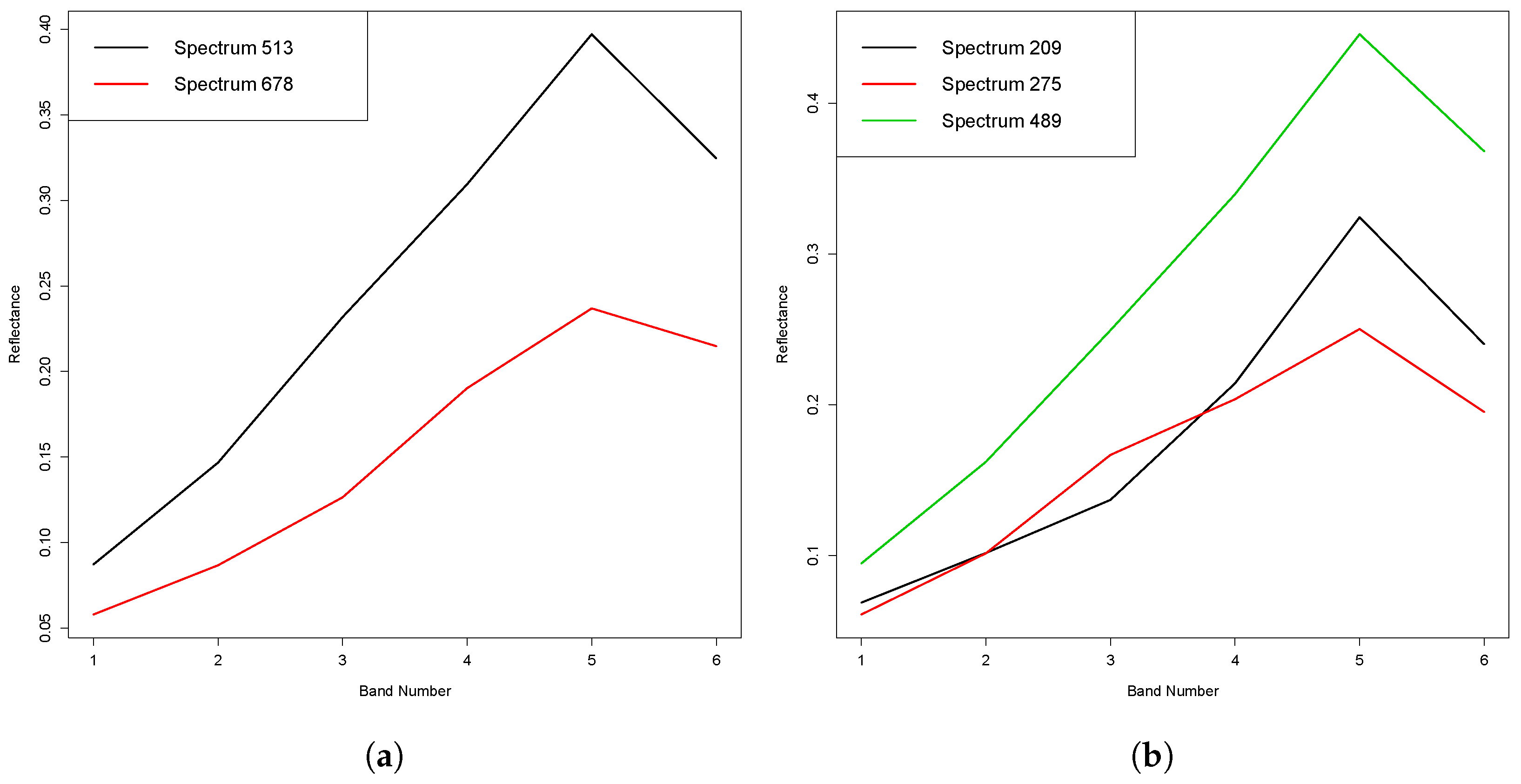
The exploratory data analyses will take two forms. The first compares spectra in the dataset with identical nominal proportions. There are eleven pairs and one triplet of spectra with identical nominal proportions. Figure 1a shows one of these pairs, spectra 513 and 678, while Figure 1b shows the triplet, spectra 209, 275 and 489. The common nominal proportions, listed as $p_{PV},p_{NPV}$ and $p_{BS}$, are given in the captions of the two plots, correct to three decimal places (although they are in fact equal to six decimal places). What stands out in these plots (and many of the other plots of pairs of spectra with identical nominal proportions) is that many spectra with the same nominal proportions have similar shapes but different average values (i.e., brightnesses or albedos). The most obvious explanation for this is a shade component in the model, which is often included in the MESMA model. Ways of modelling shade will be discussed in Section 2.2.

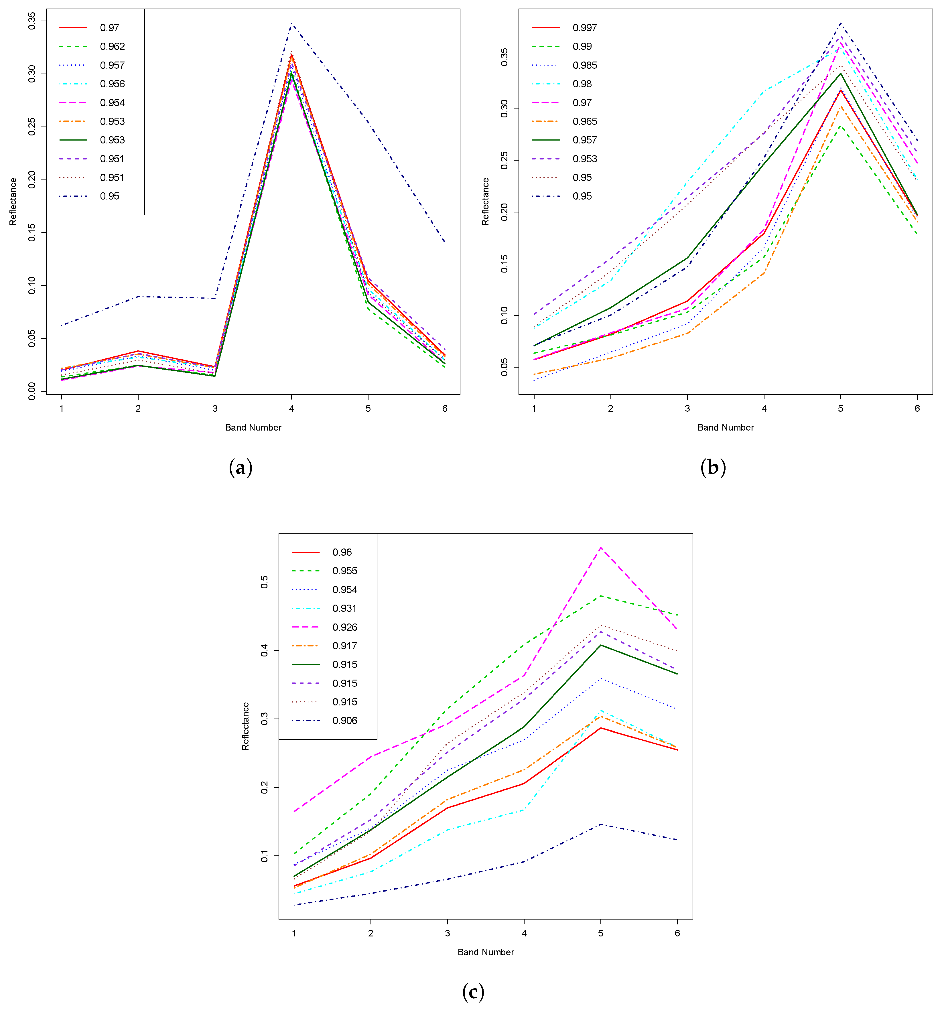
The second form of exploratory data analysis involves an examination of the nominally purest spectra (i.e., those with the largest nominal proportions) in each of the three classes. Figure 2a–c show the ten nominally purest PV, NPV and BS spectra, respectively. The nominal proportions for the dominant groundcover type of each of the spectra are shown in the top left hand corner of each of the three plots. The purest PV spectra all have their maximum value in band 4, which easily distinguishes PV spectra from NPV and BS spectra, which both have their maximum value in band 5, partly explaining the greater difficulty in discriminating between them, especially in mixtures. The nine purest PV spectra are very similar, with $0.951\le p_{PV}\le 0.970$. and $p_{BS}\le 0.002$. The tenth purest PV spectrum has $p_{PV}=0.950$ and $p_{BS}=0.044$.

By contrast, the shapes of the ten purest NPV and BS spectra are much more variable, especially in bands 1, 2 and 3. For the ten purest NPV spectra, $0.950\le p_{NPV}\le 0.997$, while for the ten purest BS spectra, $0.906\le p_{BS}\le 0.960$.

Although none of the thirty spectra are perfectly pure, they are all more than 90% pure. The greater variability of the purest NPV and BS spectra suggests that more than one endmember is required to model these. For this reason, the final model will use 1 PV, 2 NPV and 2 BS endmembers.

2.2. Two Linear Mixture Models and Error Assumptions

The linear mixture model is usually defined as follows. Let $X_i,i=1,\dots ,N$ denote the d-dimensional column vector of observations for sample i (out of N). For Landsat TM data, $d=6$. Oftentimes, the samples are contiguous spectra in a multispectral (or hyperspectral) image. Instead, the samples analysed by ([2], Figure 1) consist of 1169 spectra collected at 913 sites around Australia. Under the LMM, if there are $M(<N)$ spectrally distinct materials in the dataset, then:

$$X_i=\sum _{k=1}^M{p}_{ik}{E}_k+{ϵ}_i,i=1,\dots ,N,$$

(1)

where (i) $E_k,k=1,\dots ,M$ are the pure endmembers; (ii) $p_{ik}$ are proportions and (iii) ${ϵ}_i$ are error terms. In Section 2.3.1 and Section 2.3.2, where there is only one endmember per class, $M=3$, while in Section 2.3.3, Section 2.3.4 and Section 2.3.5, $M>3$. They will then be reduced to three endmembers in various ways.

In most of the above-mentioned papers, because the weights in (1) are interpreted as proportions, the constraints for each i are:

$$\sum _{k=1}^M{p}_{ik}=1,$$

(2)

and

$$p_{ik}\ge 0,k=1,\dots ,M.$$

(3)

This will be called the Proportion Linear (PL) model.

This model is inadequate to model the brightness variations seen in Figure 1a,b. This is often dealt with, in part, by adding a shade endmember, often modelled as zero reflectance in all bands, e.g., [20]. If this is done, (1) and (3) still hold, but (2) must be replaced by:

$$\sum _{k=1}^M{p}_{ik}\le 1.$$

(4)

This inequality will hold for all the spectra in a dataset without having to enforce it if the non-shade endmembers are sufficiently bright. This may require some manual intervention. Alternatively, quadratic programming methods ([32], Chapter 16) can be used to enforce the inequality. A simpler approach is to multiply the deterministic part of the right hand side of (1) by a positive scale factor, ${\gamma }_i$, i.e.,

$$X_i={\gamma }_i\sum _{k=1}^M{p}_{ik}{E}_k+{ϵ}_i,i=1,\dots ,N.$$

(5)

Equation (5) can be rewritten as:

$$X_i=\sum _{k=1}^M{\beta }_{ik}{E}_k+{ϵ}_i,i=1,\dots ,N,$$

(6)

where

$${\beta }_{ik}\ge 0,k=1,\dots ,M,$$

(7)

$${\gamma }_i=\sum _{k=1}^M{\beta }_{ik},i=1,\dots ,N,$$

(8)

and

$$p_{ik}={\beta }_{ik}/{\gamma }_i,k=1,\dots ,M;i=1,\dots ,N.$$

(9)

Note that the constraint (2) is no longer required. This model will, therefore, be called the Non-Negative Linear (NNL) model.

The errors in both models are typically a combination of instrumental noise, natural variation in spectra representing the same material and small non-linearities in the mixing. Typically, natural variation dominates the error ([33], Introduction). It is often assumed (implicitly or explicitly) that the errors have zero means, and are spatially and spectrally uncorrelated with a Gaussian distribution with constant variance ${\sigma }^2$. Gaussian errors will also be assumed, but for most of the paper it will be assumed that:

$$Var\left({ϵ}_{ij}\right)={\sigma }_i^2,j=1,\dots ,d;i=1,\dots ,N,$$

(10)

where ${ϵ}_i\equiv ({ϵ}_{i1},{ϵ}_{i2},\dots ,{ϵ}_{id})$. This enables different samples to have different acceptable goodness-of-fit levels, which will prove useful in Section 2.3.

While a more general (sample-dependent) variance-covariance structure than (10) can be assumed, the formulae in the paper will be more complicated. In Section 2.3.5, it is shown how the more general variance-covariance structure can be converted to (10).

Under assumption (10), the maximum likelihood estimators of the weights in both models are obtained via least squares (LS) estimation, subject to the constraints (2) and (3) for the PL model and (7) for the NNL model. These will be called the constrained estimators. It will also be useful to calculate the coefficients without the non-negativity constraints (3) or (7) imposed. These will be called the unconstrained estimators. Both the constrained and unconstrained estimators will be shown for selected examples in Section 3 using both the PL and NNL models with $M=3$, and also the NNL model with $M=5$.

2.3. Confidence Intervals and Joint Confidence Regions for Five Linear Mixture Models

In all five subsections of this section, formulae for CIs and JCRs will use a general value of M. Specific values of M (e.g., 3 and 5) will only be used where necessary, and in particular for the examples shown in Section 3. In Section 2.3.1 and Section 2.3.2, formulae will be given for the general PL and NNL models, respectively. In Section 2.3.3, the situation of primary and secondary endmembers will be discussed, while endmember variability [29] will be addressed in Section 2.3.4. The solutions in these two cases can be obtained via minor modifications of the PL and/or NNL models. In Section 2.3.5, the error variance assumption (10) will be relaxed.

In Section 2.3.1, Section 2.3.2, Section 2.3.3 and Section 2.3.4, it will usually be unnecessary to include the subscript i (the sample number), so for simplicity, it will (mostly) be omitted. It will be reintroduced in Section 2.3.5.

2.3.1. The Proportion Linear Model

This is probably the most widely used model. It is also the easiest for illustrating two important general principles, which are also applicable to the other models that will be analysed.

It will be instructive to compare two estimators, the unconstrained LS estimators of the proportions (i.e., without imposing the non-negativity constraints (3), but imposing the sum-to-one constraint (2)) and the constrained LS estimators (i.e., with both constraints (2) and (3) imposed).

The unconstrained LS estimators have been derived by ([34], eqn. (11)). Their formula assumes a general covariance matrix. This simplifies if it is assumed that the errors are uncorrelated; see (10). Using a simplified notation, their formula becomes:

$${\widehat{p}}_u={\widehat{p}}_0+\mu \mathbf{F}{\mathbf{1}}_M,$$

(11)

where ${\widehat{p}}_u^T\equiv ({\widehat{p}}_{1,u},{\widehat{p}}_{2,u},\dots ,{\widehat{p}}_{M,u})$, ${\mathbf{1}}_M$ is a vector consisting of M 1’s, $\mathbf{E}\equiv (E_1,E_2,\dots ,E_M),$

$$\mathbf{F}={\left({\mathbf{E}}^T\mathbf{E}\right)}^{-1},$$

(12)

$$\mu =(1-{\mathbf{1}}_M^T{\widehat{p}}_0)/\delta ,$$

(13)

$$\delta ={\mathbf{1}}_M^T\mathbf{F}{\mathbf{1}}_M$$

(14)

and

$${\widehat{p}}_0=\mathbf{F}{\mathbf{E}}^{T}X$$

(15)

is the standard LS estimator without either the constraints (2) and (3) imposed.

It will later be useful to know the covariance matrix of ${\widehat{p}}_u$. In the less general situation considered in this paper, ([34], eqn. (13)) simplifies to:

$$Cov\left({\widehat{p}}_u\right)={\sigma }^2\mathbf{V},$$

(16)

where

$$\mathbf{V}\equiv \mathbf{F}-\mathbf{F}{\mathbf{1}}_M{\mathbf{1}}_M^T\mathbf{F}/\delta .$$

(17)

It is straightforward to show that the residual sum of squares of the unconstrained fit, $RS{S}_{i,u}$, is given by:

$$RS{S}_u=X^T\{\mathbf{I}-\mathbf{E}\mathbf{F}{\mathbf{E}}^T\}X+{\mu }^2\delta ,$$

(18)

and that an unbiased estimator of ${\sigma }^2$ is given by ([35], eqn. (4.29)):

$${\widehat{\sigma }}^2=RS{S}_u/(d-M+1).$$

(19)

When $M=3$ and $d=6$, the denominator, the df, is $d-M+1=4$.

Unlike the unconstrained solution, the constrained solution, ${\widehat{p}}_c$ does not in general have an explicit algebraic solution. It can be obtained using quadratic programming code ([32], (Chapter 16), which is now widely available. The R package quadprog (https://cran.r-project.org/web/packages/quadprog/quadprog.pdf, accessed on 16 May 2023) has been used to produce the results in this paper. Note that, if all the elements of ${\widehat{p}}_u$ are non-negative, then both (2) and (3) are satisfied, in which case ${\widehat{p}}_u={\widehat{p}}_c$.

The first important principle will shortly be illustrated using a sample spectrum from the dataset. In order to do this, the brightness variations that are apparent in Figure 1a,b need to be removed. This will be done by dividing each spectrum by its mean value, i.e.,

$$Y\equiv X/\overline{X},$$

(20)

where

$$\overline{X}=X^T{\mathbf{1}}_d/d,$$

(21)

where ${\mathbf{1}}_d$ is a vector of d 1′s. Y will be called the standardised spectrum. It will also be convenient to assume that, for each endmember, the mean of its values is also 1, i.e.,

$$E_k^T{\mathbf{1}}_d/d=1,k=1,\dots ,M.$$

(22)

Then, it is straightforward to show ([36], Section 2.1) that, if there is no error in the NNL model (6), then the standardised spectra satisfy the PL model (1) with $p_k\equiv {\beta }_k/{\sum }_{l=1}^M{\beta }_l,k=1,\dots ,M$. Therefore, if the errors are not too large, the brightness variations can be approximately removed and a model which approximately satisfies (2) and (3) obtained by standardising both the spectra and the endmembers.

Note that, if the standardisations (20) and (22) are used, then it is necessary for Y to replace X in both (15) and (18).

In what follows, $M=3$ endmembers will be assumed. In order to satisfy (22), the standardised versions of the nominally purest PV, NPV and BS spectra shown in Figure 2a, Figure 2b and Figure 2c, respectively, will be used as the three endmembers. The first principle will be illustrated using standardised spectrum 1099 in the dataset.

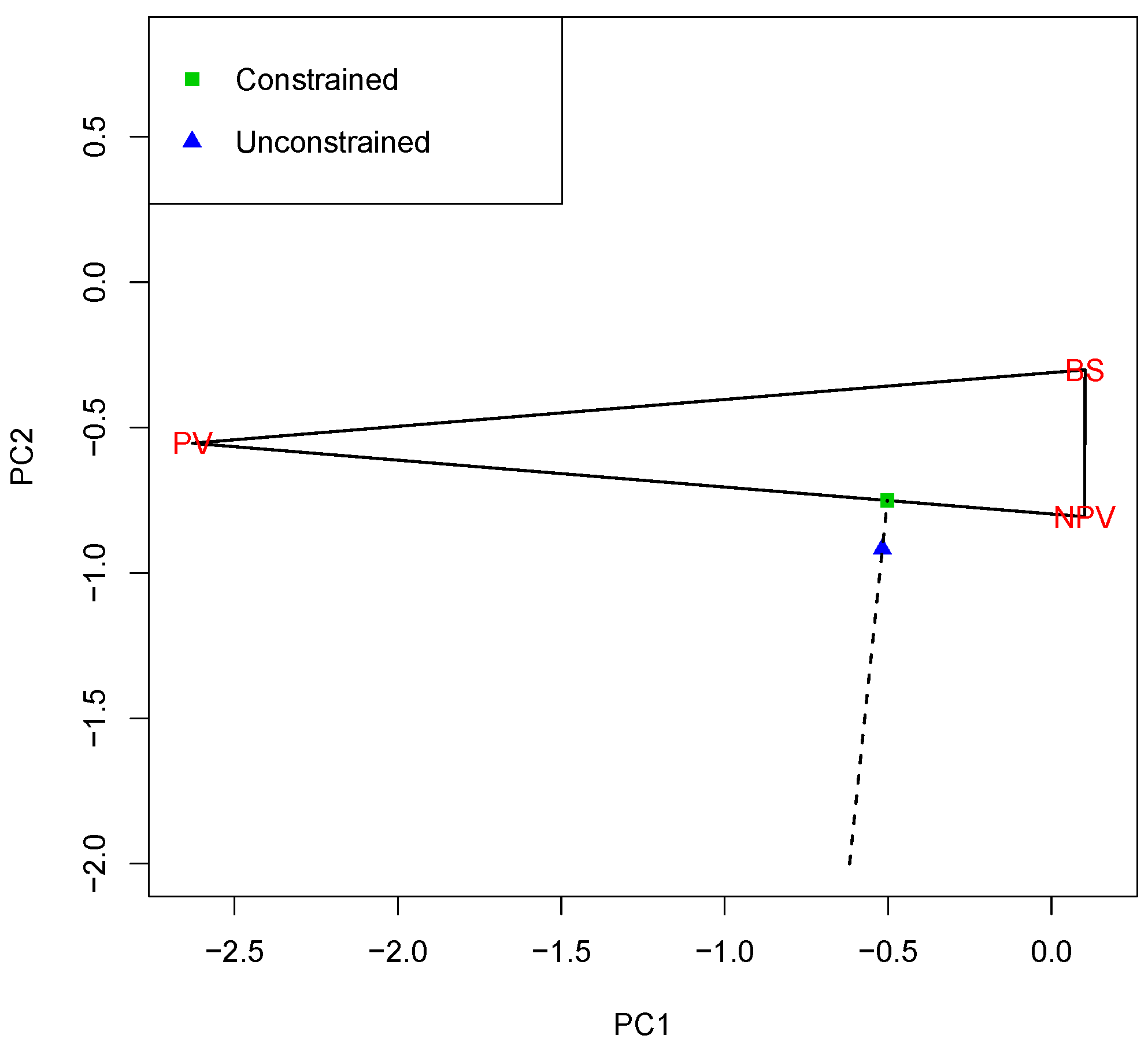
The three endmembers form the vertices of a triangle. Although this triangle lies in six-dimensional space, it can be projected onto a two-dimensional plane. This is determined by the first two Principal Components (PCs) of the three endmembers. The projected triangle is shown in Figure 3. For reasons that will shortly become clear, the lengths of the two plotting axes are equal. This figure also shows the projection of the data (Y) onto the plane determined by the endmembers (the blue triangle). This point corresponds to the unconstrained solution. Note that it lies outside the triangle. $RS{S}_u$ is just the squared distance between Y and this point. The nearest point to the blue triangle on the boundary of the triangle (the green square) is also shown. It corresponds to the constrained solution. By Pythagoras’ theorem, the RSS for the constrained fit, $RS{S}_c$, is just $RS{S}_u$ plus the squared distance between the blue triangle and the green square.

A broken line has been included between (and beyond) these two points. Because the lengths of the two plotting axes are equal, it can be seen that this broken line is perpendicular to the edge of the triangle nearest to the blue triangle. An important point to note is that all unconstrained solutions lying along the broken line have the same corresponding constrained solution. From a “confidence” perspective, if a point lies on the broken line but near the triangle, intuitively, there must be a reasonable likelihood that the “true” point lies inside the triangle. On the other hand, if the point lies on the broken line but further away from the triangle, intuitively, it is more likely that the true point actually lies on the edge of the triangle. This plot shows that, although the constrained estimator is the best point estimate consistent with the constraints, it actually throws away information. Hence, statistical inference should be based on the unconstrained estimator, which does not throw away the relevant information. This is the first major principle that this model demonstrates.

For the time being, the non-negativity constraint (3) will be ignored when considering confidence intervals and regions based on the unconstrained estimator. The confidence interval for a single proportion will be considered first. In what follows, subscripts k (or l) will be used to represent any one (or two) of the M materials. Let $v_{kl}$ denote the $(k,l)$th element of $\mathbf{V}$, given by (17). Then, by (16), ${\sigma }^2{v}_{kk}$ is the variance of ${\widehat{p}}_{k,u}$. Hence, by standard LS theory ([35], eqn. (4.54)):

$$({\widehat{p}}_{k,u}-p_k)/\left(\widehat{\sigma }\sqrt{v_{kk}}\right)$$

(23)

has a t distribution with $d-M+1$ df, and hence, (ignoring the non-negativity constraint (3)) a $100(1-\alpha )\%$ CI for $p_k$ is given by:

$${\widehat{p}}_{k,u}\pm t_{d-M+1,\alpha /2}/\left(\widehat{\sigma }\sqrt{v_{kk}}\right),$$

(24)

where $t_{d-M+1,\alpha /2}$ is the upper$100(\alpha /2)$ percentage point of the t distribution with $d-M+1$ df.

The interpretation of the CI is that it will include the true proportion, on average, $100(1-\alpha )\%$ of the time. However, the fact that the true proportion must lie in $[0,1]$ is additional information which does not invalidate this fact; it just helps us to reduce the size of the CI, without altering the fact that the true proportion lies in the CI, on average, $100(1-\alpha )\%$ of the time. Thus, the constrained CI is just the intersection of the unconstrained CI with $[0,1]$. This is the second major principle, which will be called the Intersection Principle, to be introduced in this subsection. This principle has been used previously in ([37], Section 7.2) when deriving confidence intervals for linear combinations of non-negative parameters. To the author’s knowledge, it has not been used previously for proportion estimation.

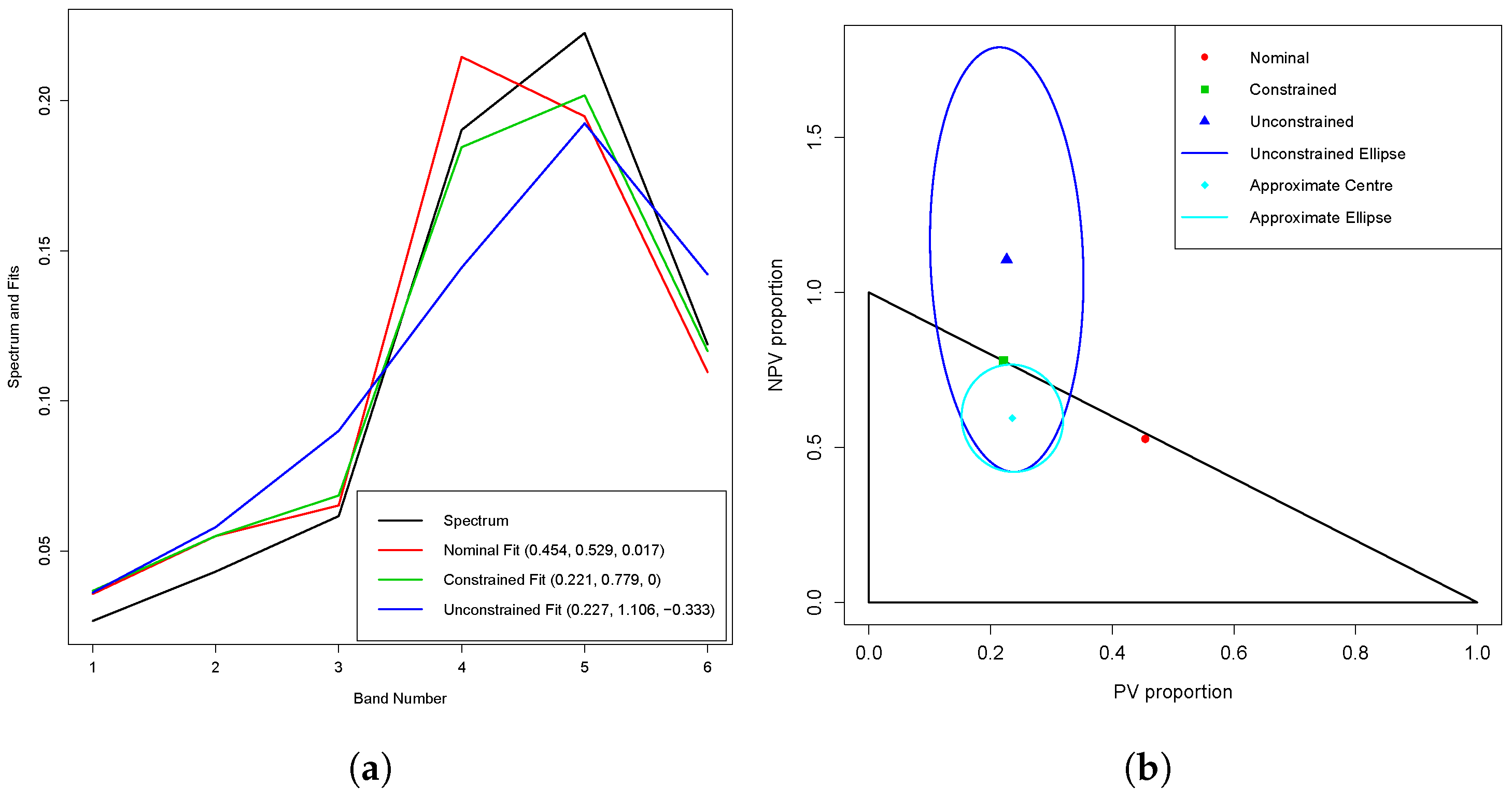
The above theory is illustrated in Figure 5a in Section 3.1, using spectrum 1099. The 95% CIs for the PV, NPV and BS proportions are (0.13, 0.32), (0.60, 1.00) and (0.00, 0.18), respectively, while the lengths of the PV and BS CIs are not too large, the length of the NPV CI is much larger. It is difficult to see how the three CIs fit together, in particular within the sum-to-one constraint (2).

The way to deal with this is to consider a joint CR for any two of the proportions; in fact, this is a JCR for all three proportions because of the sum-to-one constraint. Let $p_{kl}^T\equiv (p_k,p_l)$ denote the vector of any two proportions k and l, let ${\widehat{p}}_{kl,u}$ denote the corresponding vector of the unconstrained estimators of these two proportions and let ${\mathbf{V}}_{kl}$ denote the submatrix consisting of rows and columns k and l of $\mathbf{V}$ (given by (17)). Then, the JCR for the two proportions based on their unconstrained estimators is an ellipse given by ([35], eqn. 4.60):

$${({\widehat{p}}_{kl,u}-p_{kl})}^T{\mathbf{V}}_{kl}^{-1}({\widehat{p}}_{kl,u}-p_{kl})/\left(2{\widehat{\sigma }}^2\right)\le F_{2,d-M+1,\alpha },$$

(25)

where $F_{{\nu }_1,{\nu }_2,\alpha }$ is the upper$100\alpha$ percentage point of the F distribution with ${\nu }_1$ and ${\nu }_2$ df. It is straightforward to show that (25) is invariant to any linear transformation of the data, and thus, because of the sum-to-one constraint (2), it does not matter which two (out of three) proportion estimates are chosen.

Despite appearances to the contrary, (25) is an extension of (24). Because the latter equation is symmetric, some terms can be arranged and squared to obtain:

$${({\widehat{p}}_{k,u}-p_k)}^2/\left({\widehat{\sigma }}^2{v}_{kk}\right)\le F_{1,d-M+1,\alpha },$$

(26)

noting that $t_{d-M+1,\alpha /2}^2=F_{1,d-M+1,\alpha }$, and thus, the extension is apparent.

In Section 3.1, Figure 5b shows the nominal, constrained and unconstrained PV and NPV estimates for spectrum 1099, the 95% joint confidence ellipse for the true PV and NPV values based on (25) and the triangle determined by the constraints (2) and (3). This will be called the feasible triangle. By the intersection principle, the constrained JCR is just the intersection of the ellipse and the triangle. Although the ellipse is quite large, its intersection with the triangle is much smaller, and enables the CIs for the individual proportions to be reconciled in a coherent and interpretable way (an ellipse which approximates the JCR is also shown in cyan; this approximation will be briefly discussed in Section 2.4).

2.3.2. The Non-Negative Linear Model

In this subsection, the model (6) is assumed, and CIs and JCRs for the $p_k$’s, defined by (9), are constructed based on suitable estimators of them. These will use the two principles introduced in the previous subsection, namely the principle that statistical inference should be based on the unconstrained estimator and the intersection principle.

First, some standard LS theory is required. The unconstrained LS estimators of the coefficients in (6) are given by:

$$\widehat{\beta }=\mathbf{F}{\mathbf{E}}^{T}X.$$

(27)

where ${\widehat{\beta }}^T\equiv ({\widehat{\beta }}_1,{\widehat{\beta }}_2,\dots ,{\widehat{\beta }}_M)$. From (8) and (9), the unconstrained proportion estimates are then given by:

$${\widehat{p}}_u=\widehat{\beta }/\widehat{\gamma },$$

(28)

where

$$\widehat{\gamma }={\widehat{\beta }}^T{\mathbf{1}}_M=\sum _{k=1}^M{\widehat{\beta }}_k.$$

(29)

Again using standard LS theory, the covariance matrix of $\widehat{\beta }$ is given by:

$$Cov\left(\widehat{\beta }\right)={\sigma }^2\mathbf{F},$$

(30)

and the unbiased estimator of ${\sigma }^2$ is now given by:

$${\widehat{\sigma }}^2=X^T\{\mathbf{I}-\mathbf{E}\mathbf{F}{\mathbf{E}}^T\}X/(d-M).$$

(31)

In what follows, it will be convenient to split the vector ${\widehat{p}}_u$ into its M separate entries:

$${\widehat{p}}_{k,u}={\widehat{\beta }}_k/\widehat{\gamma },k=1,\dots ,M.$$

(32)

Note that each of the M estimators in (32) is the ratio of two random variables. When the errors have a Gaussian distribution, the general solution for the CI of a ratio is given by [38]. In Appendix A, this theory is used to derive the $100(1-\alpha )$% CI for $p_k$ under the NNL model, which is:

$$({\widehat{p}}_{k,u}-g_1{C}_k/V_{\gamma }\pm F_{1,d-M,\alpha }^{\frac{1}{2}}(\widehat{\sigma }/\widehat{\gamma })\sqrt{{\Delta }_k})/(1-g_1),$$

(33)

where

$${\Delta }_k=V_k-2{\widehat{p}}_{k,u}{C}_k+{\widehat{p}}_{k,u}^2{V}_{\gamma }-g_1(V_k-C_k^2/V_{\gamma }),$$

(34)

${\widehat{p}}_{k,u}$ is given by (32), $g_1$ is given by:

$$g_1=F_{1,d-M,\alpha }{\widehat{\sigma }}^2{V}_{\gamma }/{\widehat{\gamma }}^2,$$

(35)

and

$$V_k=f_{kk},C_k={\mathbf{f}}_k^T{\mathbf{1}}_M,V_{\gamma }=\delta ,$$

(36)

where $\delta$ is given by (14), ${\mathbf{f}}_k$ is the kth row (or column) of $\mathbf{F}$, given by (12), and $f_{kl}$ is the $(k,l)$th element of $\mathbf{F}$. It will be useful later to note that $V_k$ and $V_{\gamma }$ are proportional to the variances of the numerator and denominator in (32), respectively (see also (30)), while $C_k$ is proportional to their covariance.

There are a number of things to note about the CI (33). First, it is not centered on ${\widehat{p}}_{k,u}$, but on ${\widehat{p}}_{k,u}-g_1{C}_k/V_{\gamma }$. This is because the ratio estimator ${\widehat{p}}_{k,u}$ is a biased estimator of $p_k$. Second, for the CI to be a “valid” CI, ${\Delta }_k$ in (34) needs to be positive so that its square root in (33) is real. It is straightforward to show that, if:

$$g_1<1,$$

(37)

then ${\Delta }_k>0$. Details are not given here. This is fortuitous, because if (37) holds, then the denominator in (33) is positive. Equation (37) is satisfied by all 1169 spectra in the dataset.

The quantity $g_1$ is a useful relative goodness of fit measure. Excluding the first term on the right hand side of (35), the quantity ${\widehat{\sigma }}^2{V}_{\gamma }/{\widehat{\gamma }}^2$ is the estimated variance of $\widehat{\gamma }$ divided by ${\widehat{\gamma }}^2$ (making it scale invariant). $\widehat{\gamma }$ is the denominator in ${\widehat{p}}_{k,u}$. Thus, when the variance of the denominator is relatively large, the CI can become “invalid” (although that has not happened with any of the spectra in the dataset being considered).

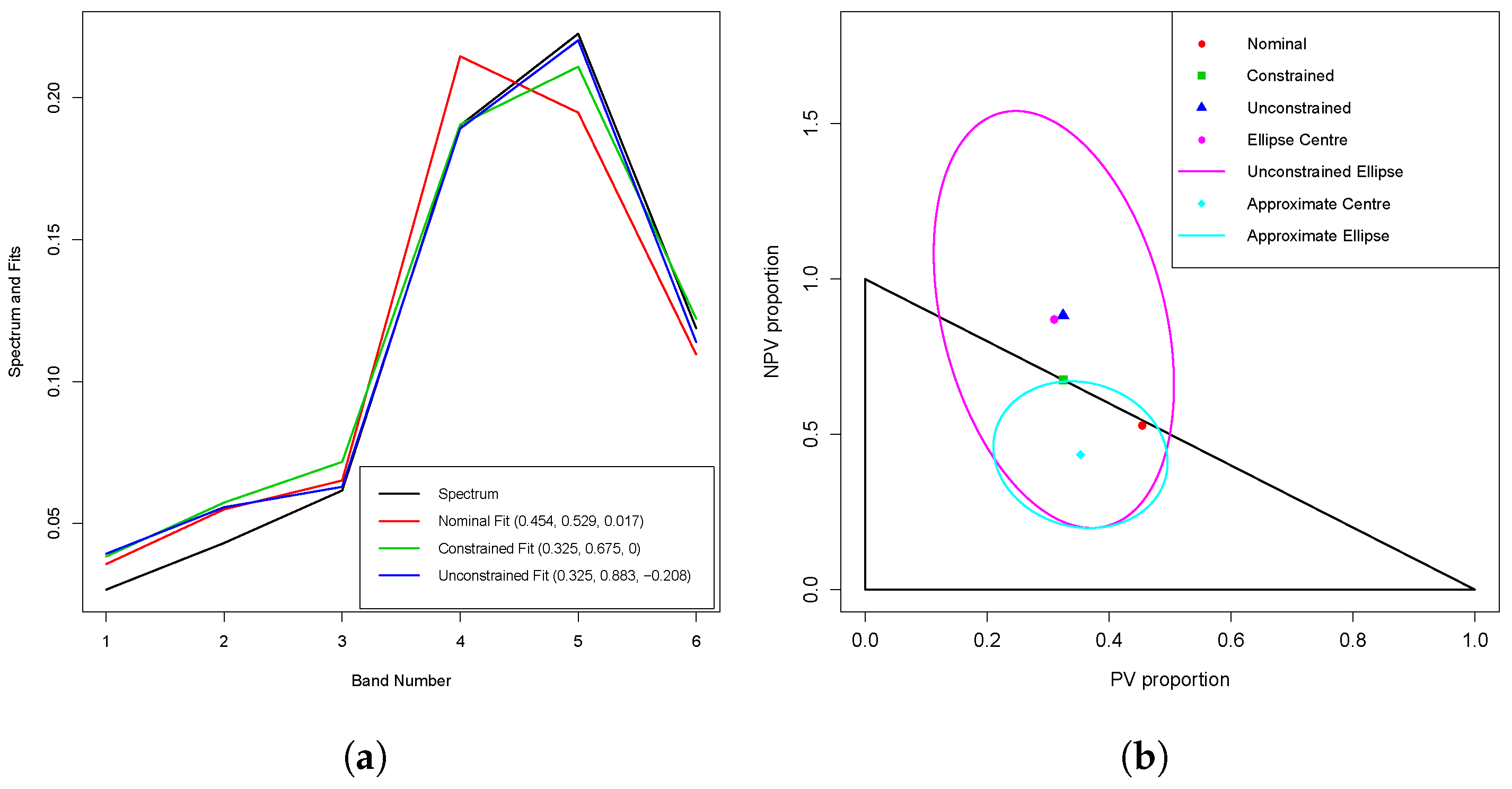
Analogous to Figure 5a under the PL model, Figure 6a in Section 3.2 shows the nominal, constrained and unconstrained fits for spectrum 1099 under the NNL model. The two fits are also compared in that section.

The JCR for any two proportions under the NNL model is now derived. As in Section 2.3.2, this is actually a JCR for all three proportions due to the sum-to-one constraint. What follows is probably original. An outline of the derivation of the JCR is given in Appendix B. A more detailed derivation will be given in a separate publication.

Let ${\widehat{p}}_{kl,u}^T\equiv ({\widehat{p}}_{k,u},{\widehat{p}}_{l,u})$ now denote a vector of two unconstrained estimators of the form (32) of $p_{kl}^T\equiv (p_k,p_l)$. The JCR based on these unconstrained estimators is based on an inequality involving a quadratic form. As pointed out previously, ${\widehat{p}}_{k,u}$ is a biased estimator of $p_k$. A consequence of this is that the quadratic form is not centered on ${\widehat{p}}_{kl,u}$. Let ${\mathbf{F}}_{kl}$ denote the submatrix consisting of rows and columns k and l of $\mathbf{F}$, and let $C_{kl}^T=(C_k,C_l)$, where $C_k$ is given by (36). Let:

$$q=p_{kl}-C_{kl}/V_{\gamma },\widehat{q}={\widehat{p}}_{kl,u}-C_{kl}/V_{\gamma }.$$

(38)

In its most succinct form, the $100(1-\alpha )\%$ JCR based on the unconstrained estimator ${\widehat{p}}_{kl,u}$ is given by those values of $p_{kl}$ satisfying:

$$q^T\mathbf{A}q+b^{T}q+c<0,$$

(39)

where

$$\mathbf{A}=\{(1-g_2)+{\widehat{q}}^T\mathbf{B}\widehat{q}\}\mathbf{B}-\mathbf{B}\widehat{q}{\widehat{q}}^T\mathbf{B},$$

(40)

$$b^T=-2{\widehat{q}}^T\mathbf{B},$$

(41)

$$c={\widehat{q}}^T\mathbf{B}\widehat{q}-g_2,$$

(42)

where

$$\mathbf{B}=V_{\gamma }{({\mathbf{F}}_{kl}-C_{kl}{C}_{kl}^T/V_{\gamma })}^{-1},$$

(43)

and

$$g_2=2F_{2,d-M,\alpha }{\widehat{\sigma }}^2{V}_{\gamma }/{\widehat{\gamma }}^2.$$

(44)

Compare (44) with (35). It can be shown that, if:

$$g_2<1,$$

(45)

then (39) is the interior of an ellipse. A proof will be published elsewhere. Compare (45) with (37). From (35) and (44):

$$g_2/g_1=2F_{2,d-M,\alpha }/F_{1,d-M,\alpha }.$$

(46)

For the data considered in this paper, $d=6$. When $M=3$ and $\alpha =0.05$, $g_2/g_1=1.89$, so that the inequality (45) is more stringent that the inequality (37). Nevertheless, all 1169 spectra satisfy the inequality (45).

Figure 6b in Section 3.2 shows the nominal, constrained and unconstrained PV and NPV estimates for spectrum 1099, the 95% joint confidence ellipse for the true PV and NPV values for the NNL model (based on (39)), the center of the ellipse and the feasible triangle.

2.3.3. Primary and Secondary Endmembers

As previously, assume that there are M endmembers, of which L are “primary” endmembers and $M-L$ are “secondary” endmembers. Without loss of generality, assume that the primary endmembers are the first L endmembers. An obvious example of this is where PV, NPV and BS are the primary endmembers, and (non-zero) shade and/or water are the secondary endmembers. In this case, the interest is in constructing CIs and JCRs for the relative proportions of the primary endmembers. The estimators of the relative proportions are just the estimators of the original proportions, divided by the sum of the original estimated proportions of the primary endmembers only. Hence, they are ratios, as are the estimated (original) proportions under the NNL model (see (28)), and thus, only small adaptations of the NNL theory are required, whether one uses the PL or NNL model to begin with. Noting the comments after (36), all that is needed is to obtain new formulae for $V_k,C_k$ and $V_{\gamma }$. The CI for the unconstrained estimators is then given by (33), while the JCR is given by (39).

Under the PL model, the relevant covariance matrix is given by (16), where $\mathbf{V}$ is given by (17). Let ${\mathbf{V}}_{L,L}$ denote the submatrix of $\mathbf{V}$ corresponding to its first L rows and L columns (corresponding to the L primary endmembers), and let ${\mathbf{v}}_{k,L}$ denote row k of ${\mathbf{V}}_{L,L}$. Then, the relevant entries in (33) and (39) under the PL model are:

$$V_k=v_{kk},C_k={\mathbf{v}}_{k,L}^T{\mathbf{1}}_L,V_{\gamma }={\mathbf{1}}_L^T{\mathbf{V}}_{L,L}{\mathbf{1}}_L,$$

(47)

where $v_{kk}$ is the kth diagonal entry of $\mathbf{V}$ (as previously defined) and ${\mathbf{1}}_L$ is a vector of $L1$’s.

Under the NNL model, the unconstrained relative estimated proportions are:

$${\widehat{p}}_{k,u}/\sum _{l=1}^L{\widehat{p}}_{l,u}={\widehat{\beta }}_k/\sum _{l=1}^L{\widehat{\beta }}_l,$$

(48)

by (32). The relevant covariance matrix is then given by (30), where $\mathbf{F}$ is given by (12). Let ${\mathbf{F}}_{L,L}$ denote the submatrix of $\mathbf{F}$ corresponding to its first L rows and L columns, and let ${\mathbf{f}}_{k,L}$ denote row k of ${\mathbf{F}}_{L,L}$. Then, the relevant entries in (33) and (39) under the NNL model are:

$$V_k=f_{kk},C_k={\mathbf{f}}_{k,L}^T{\mathbf{1}}_L,V_{\gamma }={\mathbf{1}}_L^T{\mathbf{F}}_{L,L}{\mathbf{1}}_L,$$

(49)

where $f_{kk}$ is the kth diagonal entry of $\mathbf{F}$ (as previously defined).

An example of CIs and JCRs for relative proportions of primary endmembers is not given, because the dataset in this paper does not provide any secondary endmembers. Nevertheless, it has been included because (i) it is a topic of some interest (e.g., [26,27,28]) and (ii) the relevant theory is a relatively simple extension of the NNL model.

2.3.4. Endmember Variability

This section is primarily motivated by the dataset described in Section 2.1. In particular, note that in Figure 1b, spectrum 275 is somewhat different in shape to the other two spectra, even though all three have the same nominal proportions. This is an indication that a model with unique PV, NPV and BS endmembers (such as (1) or (6)) is inadequate to model such variation.

A common approach to this endmember variability problem [29] is to use libraries with multiple examples of pure “spectra” drawn from each class. Single spectra are then drawn from each of the classes for use in the LMM in such a way that a best fit is achieved according to some criterion (e.g., MESMA). Unfortunately, the approach presented in this paper is not easy to combine with this approach; see [30] and references therein.

An alternative approach which can be useful in some circumstances is presented here. The idea is to model the endmembers in each class as linear mixtures of the extreme endmembers in that class. How one might find these extreme endmembers is discussed shortly, but for the time being, assume that they have been found. Let L now denote the number of broad classes. Within broad class $j,j=1,\dots ,L$, assume that there are $n_j$ extreme endmembers. Then, the total number of exteme endmembers is $M={\sum }_{j=1}^L{n}_j$. Error estimation is only possible if $M\le d$ under the PL model and $M<d$ under the NNL model, which is a significant limitation of the approach for small d.

Let ${\mathcal{C}}_j$ denote the indices k (between 1 and M) belonging to broad class $j,j=1,\dots ,L$. Either the PL model or the NNL model is first fitted using all M extreme endmembers, and then the proportions of each broad class are modelled as:

$$p_j^{*}=\sum _{k\in {\mathcal{C}}_j}{p}_k,j=1,\dots ,L.$$

(50)

There is an analogous formula for the unconstrained estimators of these parameters, ${\widehat{p}}_j^{*}$, based on (11) for the PL model, and (28) for the NNL model. Equation (50) can be written in matrix notation. Let $p^T=(p_1,\dots ,p_M)$ denote the vector of notionally true proportions of the M extreme endmembers, and let $p^{*T}=(p_1^{*},\dots ,p_L^{*})$ denote the L broad class proportions. Let $\mathbf{H}$ denote an $L\times M$ matrix, with entry $h_{j,k}$ in row j and column k given by:

$$\begin{array}{ccc}\hfill h_{j,k}& =& 1,k\in {\mathcal{C}}_j,\hfill \\ \hfill & =& 0,\mathrm{otherwise}.\hfill \end{array}$$

(51)

Then, the matrix version of (50) is:

$$p^{*}=\mathbf{H}p,$$

(52)

with analogous formulae for the estimated unconstrained proportions, ${\widehat{p}}_u^{*}$, under both the PL and NNL models.

For the PL model, it follows from (16) that:

$$Cov\left({\widehat{p}}_u^{*}\right)\equiv {\sigma }^2{\mathbf{V}}^{*}={\sigma }^2\mathbf{H}\mathbf{V}{\mathbf{H}}^T,$$

(53)

where $\mathbf{V}$ is given by (17). Then, the formulae given for CIs and JCRs under the PL model in Section 2.3.1 apply with $\mathbf{V}$ everywhere replaced by ${\mathbf{V}}^{*}$. Note that the formula for ${\widehat{\sigma }}^2$ (19) remains unchanged.

For the NNL model, the relevant quantity is ${\widehat{\beta }}^{*}=\mathbf{H}\widehat{\beta }$, where $\widehat{\beta }$ is given by (27). It follows from (30) that:

$$Cov\left({\widehat{\beta }}^{*}\right)\equiv {\sigma }^2{\mathbf{F}}^{*}={\sigma }^2\mathbf{H}\mathbf{F}{\mathbf{H}}^T,$$

(54)

where $\mathbf{F}$ is given by (12). Then, the formulae given for CIs and JCRs under the NNL model in Section 2.3.2 apply with $\mathbf{F}$ everywhere replaced by ${\mathbf{F}}^{*}$. Note that ${\widehat{\sigma }}^2$ is still given by (31); ${\mathbf{F}}^{*}$ does not replace $\mathbf{F}$ in this equation.

Although the above approach has limitations when d is small, its advantage is that it can often model the variety of endmembers within a broad class in a continuous way. The usual approach relies on having enough endmembers in each broad class to represent all the variability among mixtures in the dataset under consideration. This may not always be the case.

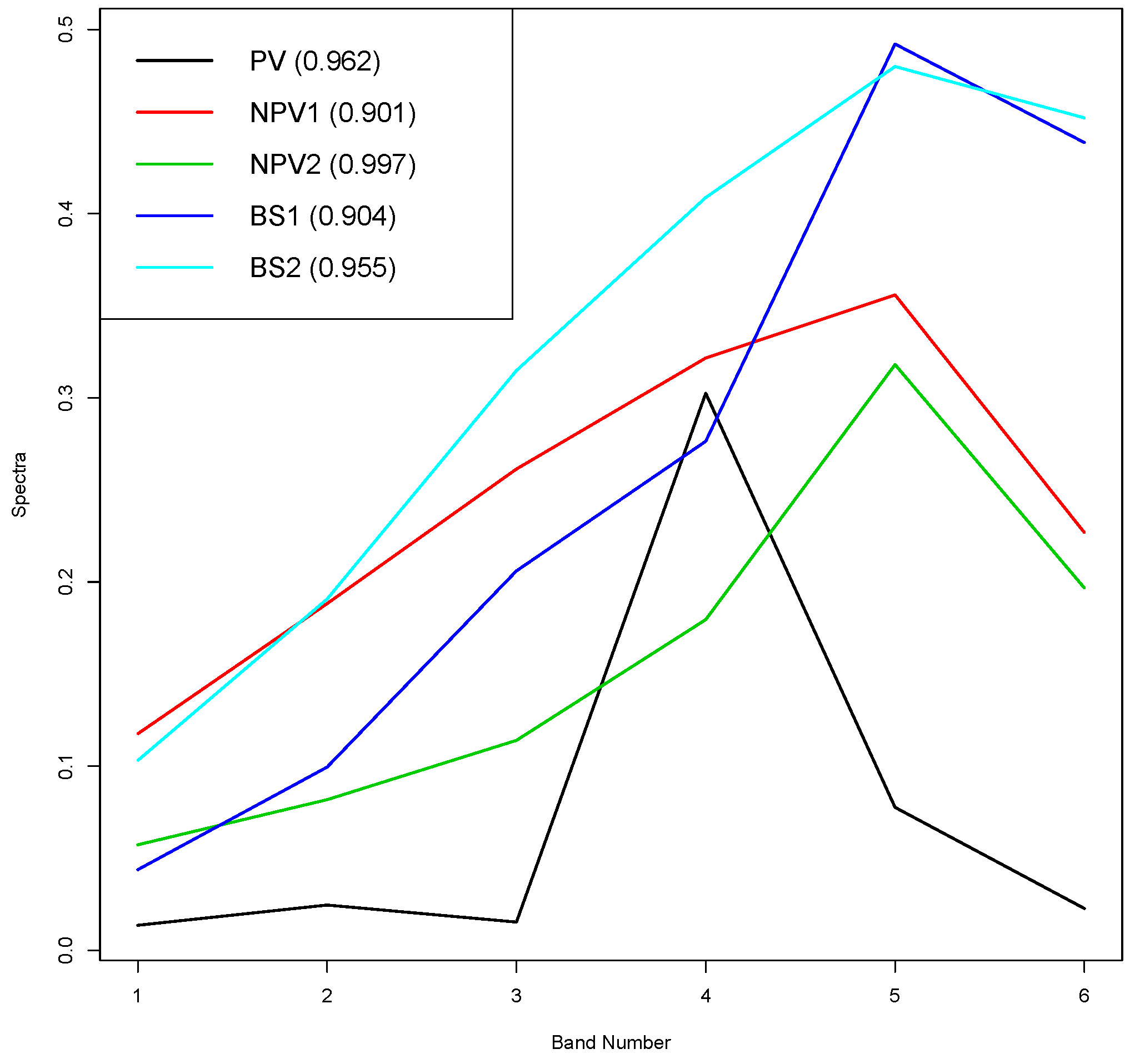
The above theory is now applied to the dataset discussed in Section 2.2 using the NNL model. Because $d=6$, there can be at most $M=5$ endmembers. The greater variability of the purest NPV and BS spectra in the dataset (see Figure 2a–c) suggests that the model should use 1 PV, 2 NPV and 2 BS endmembers. It is not easy to find extreme endmembers in the latter two broad classes using automated methods. Fortunately, there are two significant subsets of the dataset where the nominal proportion of one of the broad classes is $<0.01$ (i.e., that class is almost absent): 181 spectra (15.5% of the total) have $p_{PV}<0.01$, while 110 spectra (9.4%) have $p_{BS}<0.01$. Plots of the first few PCs of the standardised spectra of these two subsets make it relatively easy to identify suitable candidates for the extreme endmembers for all three broad classes. Details of the approach will not be given here. The five (unstandardised) endmembers found using this approach are shown in Figure 4. Their nominal proportions are shown in the legend, while one each of the PV, NPV and BS endmembers has a nominal proportion which is either the highest or second highest nominal proportion in its broad class; the other NPV and BS endmembers have much lower nominal proportions, each a little over 0.90.

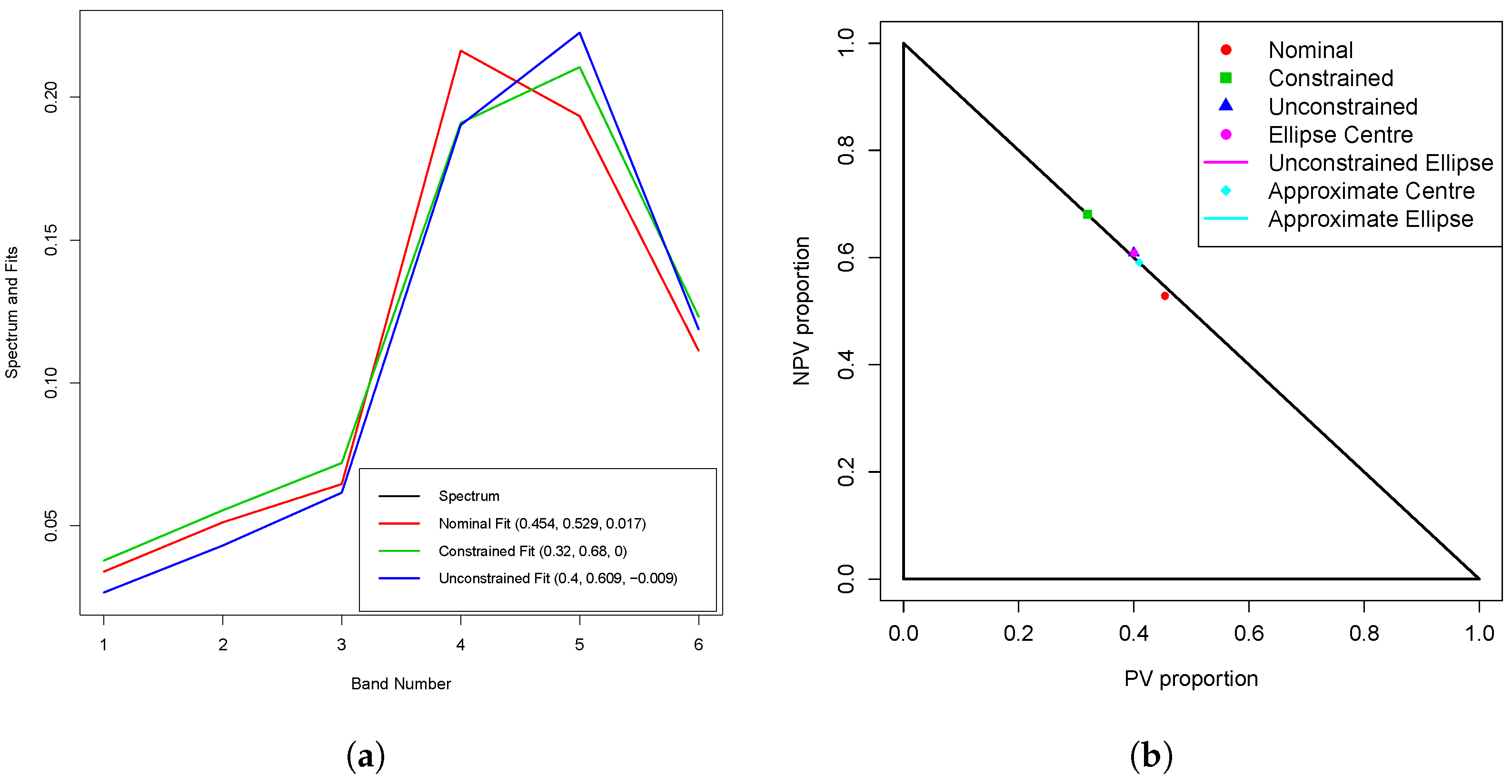
In Section 3.3, Figure 7a shows the nominal, constrained and unconstrained fits for spectrum 1099 under the five-endmember NNL model, while the corresponding JCR is shown in Figure 7b.

Unfortunately, there is a downside to the use of the five-endmember NNL model. Whereas all 1169 spectra satisfy the inequalities (37) and (45) (which are sufficient to ensure valid (unconstrained) CIs and JCRs) for the three-endmember NNL model, only 1101 and 926 of the spectra satisfy these inequalities, respectively, for the five-endmember NNL model. At first glance, this may appear contradictory, because one would expect a better fit of the five-endmember model than for the three-endmember model. Indeed, for 1093 of the 1169 spectra (93.5%), ${\widehat{\sigma }}^2$, defined by (31), is smaller for the five-endmember model than it is for the three-endmember model. The reason that it is not 100% is partly because the endmembers in the three-endmember model are not a subset of the endmembers in the five-endmember model, but more importantly because the denominator in (31) (the df) is reduced from 3 to 1, so the five-endmember numerator needs to be considerably smaller than the three-endmember numerator to counteract this. In addition, note that in the definitions of $g_1$ and $g_2$ ((35) and (44), respectively), there are a number of factors, apart from ${\widehat{\sigma }}^2$, that will change between the two models, in particular the factor $F_{l,d-M,\alpha }$, where $l=1$ or 2 for $g_1$ and $g_2$, respectively. These factors are much higher when $d-M=1$ than when $d-M=3$. For instance, $F_{1,1,0.05}/F_{1,3,0.05}=15.9$, while $F_{2,1,0.05}/F_{2,3,0.05}=20.9$. Thus, the other factors in $g_1$ and $g_2$ have a lot of work to do when the df is reduced from 3 to 1.

In the next section, it is shown how this problem can be ameliorated somewhat.

2.3.5. Relaxing the Variance Equality Assumption (10)

In this section, it will be convenient to reintroduce the subscript i to represent spectrum i.

Up to this point, it has been assumed that the errors in each band of any spectrum have the same variance and are uncorrelated; see (10). An examination of the ten purest PV, NPV and BS spectra (Figure 2a–c, respectively) suggests that perhaps there is greater variability in bands 1, 2 and 3 than in bands 4, 5 and 6. Thus, perhaps the assumption (10) should be relaxed. Although this will be done shortly, for the sake of completeness, (10) will be generalised to:

$$Cov\left({ϵ}_i\right)={\sigma }_i^2\Omega ,i=1,\dots ,N,$$

(55)

where $\Omega$ is assumed known, but ${\sigma }_i$ is assumed unknown. It is straightforward to convert any of the three models considered so far with the assumption (55) into the analogous model with the assumption (10). This is done via an eigendecomposition of $\Omega$:

$$\Omega =Q^T\Lambda Q,$$

(56)

where

$$Q^{T}Q=I.$$

(57)

Here, $\Lambda$ is the diagonal matrix of eigenvalues of $\Omega$ (which will all be assumed positive), and the columns of Q are its eigenvectors. Let:

$$Z_i={\Lambda }^{-1/2}Q{X}_i.$$

(58)

It follows easily from (56) and (57) that $Z_i$ satisfies (10). Thus, the theory of the previous four subsections will apply if $X_i$ is first transformed to $Z_i$ via (58).

In principle, with a large enough library of pure spectra, it should be possible to estimate $\Omega$ and to then use the transformation (58); see for instance [10].

This is not the case with the dataset discussed in Section 2.2. Some progress is possible if one is prepared to assume that $\Omega$ is diagonal, i.e., the errors in different bands are uncorrelated (note that in this case, $Q=I$ and $\Lambda =\Omega$). This will be called the variable error variance model, and the model (10) the constant error variance model. Denote the diagonal entries of $\Omega$ by ${\omega }_1,{\omega }_2,\dots ,{\omega }_d$. For the five-endmember NNL model, a relatively simple, if crude, method to estimate these is as follows. For spectrum i, consider the vector of residuals obtained from the constant error variance model ${\rho }_i=({\rho }_{i1},{\rho }_{i2},\dots ,{\rho }_{id})$, given by:

$${\rho }_i=X_i-E{\widehat{\beta }}_i,$$

(59)

where ${\widehat{\beta }}_i$ is given by (27). If ${\rho }_{ij}$ is squared, each should on average be approximately proportional to ${\omega }_j$. However, brighter spectra will tend to have larger residuals than darker spectra, so ${\rho }_{ij}^2$ should be divided by ${\widehat{\gamma }}_i^2$, given by (29), and then this statistic should be averaged over all the fitted spectra in the dataset, i.e.,

$${\omega }_j=\sum _{i=1}^N{\rho }_{ij}^2/{\widehat{\gamma }}_i^2,j=1,\dots ,d.$$

(60)

This has been done for the five endmember model and all 1164 non-endmember spectra. The values of ${\omega }_j^{1/2}(\times {10}^{-5})$ (the actual divisors of each entry of $X_i$) are: 271, 368, 147, 12.5, 4.1, 16.1. As expected, these are much larger for bands 1, 2 and 3 than they are for bands 4, 5 and 6.

When these values are used to produce $Z_i$, instead of $X_i$ (Equation (58)), the number of spectra satisfying (37) increases from 1101 (94.2%) to 1169 (100%), while the number of spectra satisfying (44) increases from 926 (79.2%) to 1148 (98.2%).

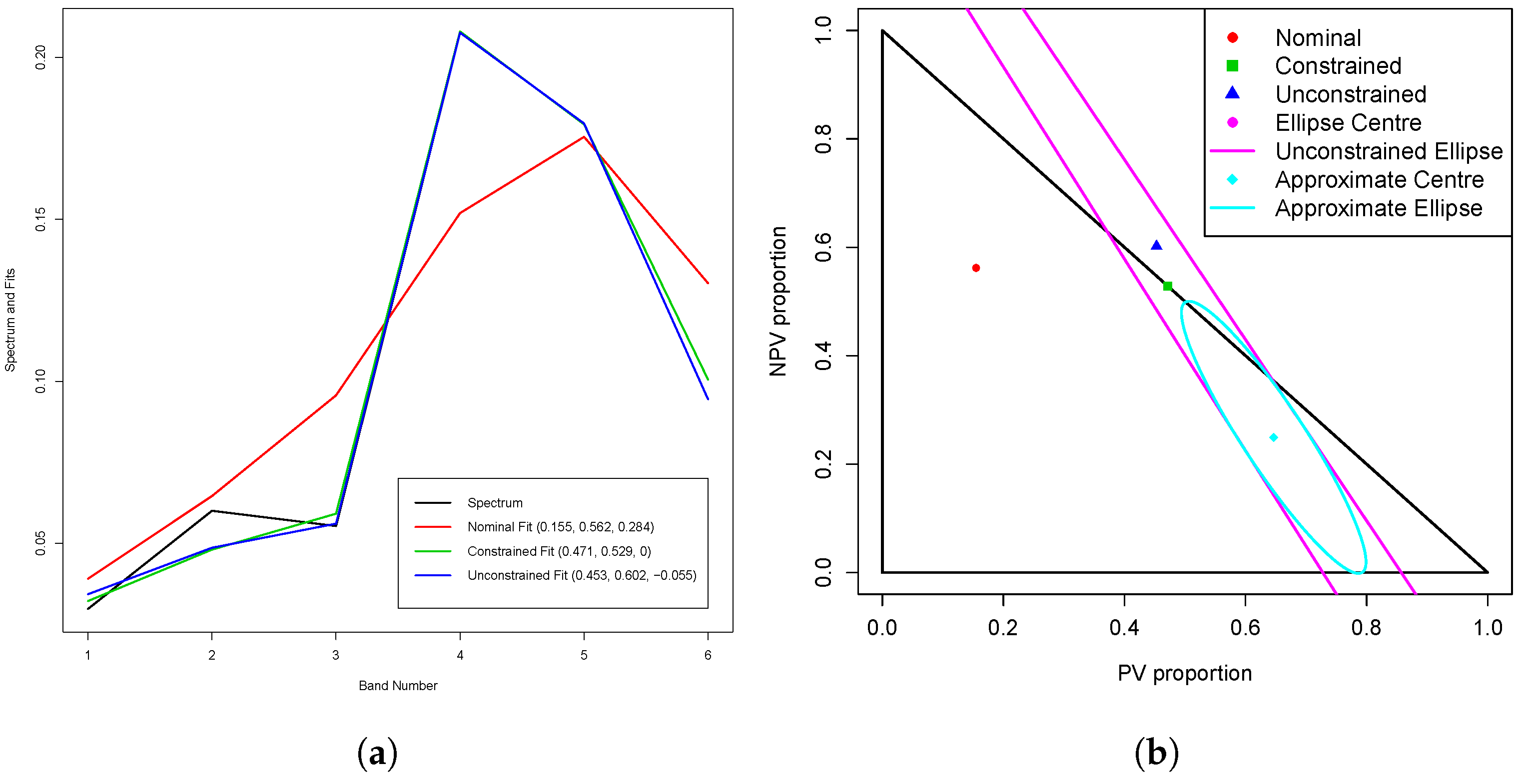
As an example of this transformation, in Section 3.4, the fits and JCR for spectrum 77, the spectrum with the largest value of $g2$ less than 1 (0.995), are shown.

2.4. Application to Multispectral Image Data

The intersection of an ellipse and a triangle cannot be represented algebraically. This is a drawback if one has multispectral image data. Such data are themselves usually summarised by a smaller number of images (e.g., NDVI images) for ease of interpretation. It would, therefore, be useful if the JCR (which, as can be seen in various examples above, is much more informative than three separate CIs) could be approximated by a small number of parameters which can be displayed as color images.

The basic idea presented in this section is to approximate the JCR itself by an ellipse. The “approximating” ellipse will be differentiated from the ellipse intersecting the feasible triangle by calling the latter the “unconstrained” ellipse. Examples of the approximating ellipse are shown (in cyan) in Figure 5b–8b.

Although the idea is easy to explain, there are a number of ways in which an ellipse can (or cannot) intersect a triangle, and it can be tedious to implement them all. The vast majority of examples fall into one of five categories. Three of these categories have been illustrated in this paper. Figure 5 and 6b exemplify the category where the unconstrained ellipse intersects the boundary of the triangle in two places and has one end inside and one end outside the triangle. Figure 7b exemplifies the category where the unconstrained ellipse does not intersect the triangle at all. Figure 8b exemplifies the category where the unconstrained ellipse intersects the boundary of the triangle in four places. The two other main categories are: (i) the unconstrained ellipse lies entirely inside the feasible triangle and (ii) one edge of the unconstrained ellipse intersects the boundary of the triangle in two places (on two different sides), but both ends are outside the triangle. Typically, this happens near a corner of the feasible triangle.

An example of this category is shown in ([39] Section 5.1). Rare pathological examples have also been found in the dataset discussed in this paper, as well as two other datasets. One of these pathological examples is also shown in ([39] Section 5.1).

As the examples shown in this paper illustrate, the approximating ellipse usually provides a reasonable approximation to the intersection of the unconstrained ellipse and the feasible triangle.

Once the major and minor axis lengths and the orientation of the approximating ellipse have been calculated at each pixel, they can be displayed as a color image, as can three proportion estimates, either the constrained estimates or the centers of the approximating ellipse. There is extensive discussion about this issue in ([39] Section 5.2). Various issues are illustrated with the aid of two small image datasets.

3. Results

In this section, examples of the use of the theory introduced in Section 2.3.1, Section 2.3.2, Section 2.3.4 and Section 2.3.5 are shown. Spectrum 1099 is used to illustrate differences in the fits, CIs and JCRs using the models in the first three subsections. For the model used in Section 2.3.5, the spectrum with the largest value of $g_2<1\left(0.995\right)$ is spectrum 77. Its fits, CIs and JCR are also shown in the last subsection.

3.1. Three-Endmember Proportion Linear Model

Figure 5a shows the nominal, constrained and unconstrained fits for spectrum 1099 using the standardised versions of the nominally purest PV, NPV and BS spectra shown in Figure 2a–c, respectively, as the $M=3$ endmembers. The corresponding PV, NPV and BS proportions are shown in the legend, while the corresponding 95% confidence intervals (based on (24) and the intersection principle) are given in the caption. There are a number of things to note. First, the constrained fit is fairly good (it gets better as the model becomes more sophisticated). Second, the nominal fit is much poorer because the nominal PV and NPV proportions are, respectively, significantly higher and lower than the corresponding constrained estimates. Third, the unconstrained fit is poorer still.

Figure 5b shows the nominal, constrained and unconstrained PV and NPV estimates for spectrum 1099, the 95% joint confidence ellipse for the true PV and NPV values based on (25) and the triangle determined by the constraints (2) and (3). The constrained JCR is just the intersection of the ellipse and the triangle.

3.2. Three-Endmember Non-Negative Linear Model

Analogous to Figure 5a under the PL model, Figure 6a shows the nominal, constrained and unconstrained fits for spectrum 1099 under the NNL model. As in the previous subsection, the nominally purest PV, NPV and BS spectra (shown in Figure 2a–c, respectively) have been used as the three endmembers. However, unlike in the previous subsection, none of the endmember spectra have been standardised. As previously, the constrained solution can be found using quadratic programming methods ([32], Chapter 16). For bands 1, 2 and 3, the constrained fit under the NNL model is a little worse than the constrained fit under the PL model. It is much better for bands 4, 5 and 6. On the other hand, the unconstrained fit under the NNL model is clearly far superior to its counterpart under the PL model. This example clearly illustrates the advantage of fitting the NNL model, rather than standardising the spectra first and then fitting the PL model.

Although the unconstrained fit under the NNL model is visually much better than its counterpart under the PL model, the 95% CIs are somewhat longer; see the captions for Figure 5 and Figure 6 for detaxils. Although this is perhaps disappointing, it is probably more realistic.

Figure 6b shows the nominal, constrained and unconstrained PV and NPV estimates for spectrum 1099, the 95% joint confidence ellipse for the true PV and NPV values for the NNL model (based on (39)), the center of the ellipse and the feasible triangle. The X and Y ranges of the figure are the same as those for Figure 5b (using the PL model), which allows for a direct comparison between the two. There are a number of things to note. First, while under the PL model, the axes of the ellipse are approximately parallel to the X and Y axes, under the NNL model, the ellipse is tilted. Second, the latter ellipse is somewhat shorter and fatter than the former. Third, ${\widehat{p}}_{PV,u}$ has increased from 0.227 to 0.325. Together, these three facts mean that the nominal proportions are now inside the confidence ellipse (and the JCR), where they were not previously. Furthermore, note the small difference between the center of the ellipse and the unconstrained estimator, due to the bias of the latter.

3.3. Five-Endmember Non-Negative Linear Model

Figure 7a shows the nominal, constrained and unconstrained fits for spectrum 1099 under the five-endmember NNL model discussed in Section 2.3.4. Compare this with the corresponding fits under the three-endmember NNL model in Figure 6a; while the constrained fit has not changed much (with the three proportions changing marginally from (0.325, 0.675, 0) to (0.320, 0.680, 0)), the unconstrained fit is now almost visually perfect (with the three proportions changing from (0.325, 0.883, −0.208) to (0.400, 0.609, −0.009)). This in turn means that $\widehat{\sigma }$ is very small, which in turn means that the 95% CIs are also very small. In fact, it is so small, that the unconstrained CI for BS does not intersect [0, 1]. If $p_{BS}=0$, one would expect this to happen about 2.5% of the time; another 2.5% of the time, the CI will intersect [0, 1] but exclude 0. There are two ways of dealing with this. First, one can reduce $\alpha$ (and hence, expand the CI) until the CI intersects [0, 1]. Alternatively, the CI is just set to the nearest value in [0, 1], i.e., [0, 0], which is what has been written in the caption of Figure 7.

This problem is reflected in the 95% JCR, which is shown in Figure 7b. The confidence ellipse is slightly outside the triangle determined by the constraints. Nevertheless, the plot gives us a good idea of where the true proportions are likely to be with a high level of confidence. More generally, the use of the five-endmember NNL model has considerably improved the fit over that produced by the three-endmember NNL model, at least for this spectrum.

Spectrum 1099 has been chosen as the exemplar in this and the previous two subsections for a number of reasons: (i) the unconstrained estimator lies outside the triangle determined by the constraints under all three models examined, (ii) the unconstrained fit under the five-endmember NNL model is significantly better than the fit under the three-endmember NNL model and (iii) under the five-endmember NNL model, the 95% CI and JCR do not intersect [0, 1] and the feasible triangle, respectively.

3.4. Relaxing the Variance Equality Assumption (10)

For spectrum 1099, the unconstrained estimators for the variable error variance model are the same as they are for the constant error variance model (to three decimal places): (0.400, 0.609, −0.009), while the constrained estimators change a little from (0.320, 0.680, 0.000) to (0.285, 0.715, 0.000). The CI and JCR (based on the unconstrained estimators) are also very similar to those shown in Figure 7a,b, respectively, so they are not shown here.

Instead, the analogous figures for spectrum 77 are shown in Figure 8a,b. This is the spectrum with the largest value of $g_2$ less than 1 (0.995). Both the unconstrained and constrained estimators fit the spectrum quite well, except in band 2, the green (chlorophyll) band. This raises three issues. First, the green peak in Figure 8a is much higher than the corresponding peaks of the ten purest PV spectra in the dataset; see Figure 2a. Thus, they are not sufficiently representative of “very green” PV spectra. The second issue is that, even if such samples were present in the dataset, both “green” and “very green” endmembers would be needed, but then df = 0, and thus, it would be impossible to generate CIs and JCRs. The third issue is that the nominal fit is much poorer, raising doubts about the accuracy of the nominal proportions. Unfortunately, because of the (relatively) poor fit in band 2, the individual 95% CIs for the three proportions are each [0, 1], which is totally uninformative. On the other hand, the JCR (shown in Figure 8b) is much more informative. The confidence ellipse is long and narrow, so only the vicinity of the feasible triangle is shown. It intersects with a relatively small part of the triangle, and thus, localises the JCR considerably. This example is a very good demonstration of the value of the JCR over the individual CIs.

In this Section, spectra 1099 and 77 have been used to illustrate several issues. Note that, for both spectra, the nominal fits are quite different to both the constrained and unconstrained fits, even under the five-endmember NNL model. This casts some doubt on the accuracy of the nominal proportions, most probably due to temporal differences between the field and remote sensing data. On the other hand, it should also be noted that there are many spectra in the dataset where the nominal and estimated proportions are in much better agreement.

4. Discussion

In this paper, two three-endmember LMMs have been analysed. In Section 2.3.1, the PL model, which assumes that the coefficients in the model are proportions, was analysed. Unless the spectra in the dataset discussed in Section 2.1 are first standardised, this model does not fit the spectra very well because of brightness variations in spectra with the same nominal PV/NPV/BS proportions; see Figure 1a,b. In order to overcome this problem, the NNL model (6) was introduced and analysed in Section 2.3.2. In this model, the coefficients are still constrained to be non-negative, but they are no longer constrained to sum to 1. The proportions are then estimated via ratio estimators. CIs and JCRs were derived for both models.

In the following three subsections, three variants of these two fundamental models were analysed. The case where there are three primary endmembers and some secondary endmembers (i.e., of lesser interest) was considered in Section 2.3.3. In Section 2.3.4, it was demonstrated how in some cases, endmember variability can be modelled under either the PL or NNL framework. This was exemplified using an NNL model with 1 PV, 2 NPV and 2 BS endmembers. In Section 2.3.5, it was shown how to relax the variance equality assumption (10).

The theory in Section 2.3.1, Section 2.3.2, Section 2.3.4 and Section 2.3.5 was illustrated with examples in Section 3.1, Section 3.2, Section 3.3 and Section 3.4, respectively.

The main difficulty with the NNL model is that the CI and JCR are only “valid” if certain conditions are satisfied. This happens when the unconstrained estimator is not sufficiently well fitted. Sufficient conditions for the CI and JCR to be valid are given by (37) and (45), respectively.

These two inequalities highlight the fact that, for the NNL model, the issue is essentially a df ($=d-M$) problem. For the three-member NNL model (with df = 3), all 1169 spectra in the exemplar dataset satisfy both inequalities when using a basic three-endmember model (in Section 2.3.2). On the other hand, when using the five-endmember model (with df = 1, in Section 2.3.4), not all the spectra satisfy the inequalities, although the situation is improved somewhat in Section 2.3.5 by using a more suitable error covariance structure.

The PL model has two apparent advantages over the NNL model. First, the CI and JCR formulae in Section 2.3.1 are always “valid”, while for the NNL model, they are only valid if (37) and (45), respectively, are satisfied. Second, for the NNL model, it is required that $M<d$, while for the PL model, it is required that $M\le d$, so an extra endmember can always be fitted using the PL model.

However, there are two problems with the PL model. First, because of brightness variations (often due to the presence of shade), both the data and the endmembers usually need to be standardised for the PL model to produce adequate fits to the data, and this induces correlations between the errors in the model. This in turn leads to differences in the shapes of the ellipses used to produce the JCR; compare the unconstrained ellipses in Figure 5b and Figure 6b. A more serious problem occurs if the endmember spectra for some (pure) classes are significantly brighter than those in other classes (which is often the case). The standardisation that is usually necessary to use the PL model forces the means of all the endmember spectra to be equal (to 1), and this will make the estimated proportions completely wrong.

The bounds $M<d$ for the NNL model and $M\le d$ for the PL model can be overcome by using a sensor with additional bands. Obvious sensors are SENTINEL-2 and MODIS (at least the seven bands with 500 m resolution or better). Airborne hyperspectral sensors such as AVIRIS and HyMap (with 224 and 126 bands, respectively) provide much greater redundancy in modelling, and hence, degrees of freedom. In such a case, the chances of the inequalities (37) and (45) being satisfied are greatly increased; see the discussion at the end of Section 2.3.4.

A related issue is that, in larger images, M will tend to be larger than it is in smaller images. The inequalities in the previous paragraph will, therefore, limit the applicability of both the PL and NNL images if d is not large enough. Again, hyperspectral image data will usually not be bound by such a limitation.

Hyperspectral sensors also (potentially) provide an opportunity to examine JCRs for more than three materials, even when some of these materials are considered to be variants within the same endmember class, using the theory presented in Section 2.3.4 and Section 2.3.5. There are two issues to address here. First, there is the visualisation issue. When there are four (possibly broad) classes, because of the sum-to-one constraint (2), the JCR will need to be displayed in 3D, which is possible because of the ready availability these days of 3D visualisation software. Visualising JCRs for more than four materials is more difficult. However, there is a more fundamental issue: is the necessary theory available to obtain JCRs for more than three materials? For the PL model, it is straightforward to generalise (25) provided $M\le d$. No such theory has been published for the NNL model for more than three materials. It is possible to generalise (39), using fairly sophisticated matrix algebra, provided $M<d$. The relevant theory will be published elsewhere.

Returning to the multispectral case, the JCR is just the intersection of the unconstrained ellipse and the feasible triangle (when they intersect). This intersection cannot be represented algebraically, which presents difficulties when summarising the information in multispectral image data. Thus, in Section 2.4, there is a discussion about how to approximate the intersection by another ellipse. The parameters of the approximating ellipse can be summarised by two color images, one representing the center of the approximating ellipse, and the other the orientation and major and minor axis lengths of the ellipse. A more detailed discussion of these issues, with some examples, can be found in [39] (Section 5).

Finally, it should be pointed out that the research presented in this paper has not shown how to use the CIs and JCRs for the proportions of interest to monitor environmental change. This will almost certainly be based on the differences between successive unconstrained estimates of corresponding proportions. However, it is not clear if and how the information contained in the feasible triangle should be incorporated into the accuracy estimates of these differences. This will be the subject of future research.

5. Conclusions

As far as the author is aware, the only papers in the remote sensing literature which have introduced new methods for assessing the accuracy of proportions from spectra are [1] and [34]. In this paper, the work in [34] has been extended.

The most significant contributions of this paper are:

• The introduction of two principles on which the CIs and JCRs are based. The first is the principle that they should be based on the unconstrained estimator (i.e., ignoring the non-negativity constraints (3) for the PL model and (7) for the NNL model) because the constrained estimator throws away important information about the variability of the estimator; see Figure 3. The second principle is called the Intersection Principle.
• Because of these constraints and the constraint (2) for the PL model, CIs do not always provide very useful information. It is demonstrated how JCRs can often overcome this issue; see for instance Figure 5a,b, Figure 6a,b and Figure 8a,b (and the captions of these figures).
• The derivation of the JCR for the NNL model. The derivation for more than three endmembers will be published elsewhere.

References

1. Asner, G.P.; Heidebrecht, K.B. Spectral unmixing of vegetation, soil and dry carbon cover in arid regions: Comparing multispectral and hyperspectral observations. Int. J. Remote Sens. 2002, 23, 3939–3958. [Google Scholar] [CrossRef]
2. Guerschman, J.P.; Scarth, P.F.; McVicar, T.R.; Renzullo, L.J.; Malthus, T.J.; Stewart, J.B.; Rickards, J.E.; Trevithick, R. Assessing the effects of site heterogeneity and soil properties when unmixing photosynthetic vegetation, non-photosynthetic vegetation and bare soil fractions from Landsat and MODIS data. Remote Sens. Environ. 2015, 161, 12–26. [Google Scholar] [CrossRef]
3. Gill, T.K.; Phinn, S.R. Improvements to ASTER-derived fractional estimates of bare ground in a savanna rangeland. IEEE Trans. Geosci. Remote Sens. 2009, 47, 662–670. [Google Scholar] [CrossRef]
4. Guerschman, J.P.; Hill, M.J.; Renzullo, L.J.; Barrett, D.J.; Marks, A.S.; Botha, E.J. Estimating fractional cover of photosynthetic vegetation, non-photosynthetic vegetation and bare soil in the Australian tropical savanna region upscaling the EO-1 Hyperion and MODIS sensors. Remote Sens. Environ. 2009, 113, 928–945. [Google Scholar] [CrossRef]
5. Ridd, M.K. Exploring a VIS (vegetation-impervious surface-soil) model for urban ecosystem analysis through remote sensing: Comparative anatomy for cities. Int. J. Remote Sens. 1995, 16, 2165–2185. [Google Scholar] [CrossRef]
6. Ward, D.; Phinn, S.R.; Murray, A.T. Monitoring growth in rapidly urbanizing areas using remotely sensed data. Prof. Geogr. 2000, 52, 371–386. [Google Scholar] [CrossRef]
7. Phinn, S.; Stanford, M.; Scarth, P.; Murray, A.; Shyy, P. Monitoring the composition of urban environments based on the vegetation-impervious surface-soil (VIS) model by subpixel analysis techniques. Int. J. Remote Sens. 2002, 23, 4131–4153. [Google Scholar] [CrossRef]
8. Wu, C.; Murray, A.T. Estimating impervious surface distribution by spectral mixture analysis. Remote Sens. Environ. 2003, 84, 493–505. [Google Scholar] [CrossRef]
9. Weng, Q.; Lu, D. Landscape as a continuum: An examination of the urban landscape structures and dynamics of Indianapolis City, 1991–2000, by using satellite images. Int. J. Remote Sens. 2009, 30, 2547–2577. [Google Scholar] [CrossRef]
10. Xu, F.; Cao, X.; Chen, X.; Somers, B. Mapping impervious surface fractions using automated Fisher transformed unmixing. Remote Sens. Environ. 2019, 232, 111311. [Google Scholar] [CrossRef]
11. Duncan, J.; Stow, D.; Franklin, J.; Hope, A. Assessing the relationship between spectral vegetation indices and shrub cover in the Jornada Basin, New Mexico. Int. J. Remote Sens. 1993, 14, 3395–3416. [Google Scholar] [CrossRef]
12. Carlson, T.N.; Ripley, D.A. On the relation between NDVI, fractional vegetation cover, and leaf area index. Remote Sens. Environ. 1997, 62, 241–252. [Google Scholar] [CrossRef]
13. Van Leeuwen, W.; Huete, A. Effects of standing litter on the biophysical interpretation of plant canopies with spectral indices. Remote Sens. Environ. 1996, 55, 123–138. [Google Scholar] [CrossRef]
14. Asner, G.P. Biophysical and biochemical sources of variability in canopy reflectance. Remote Sens. Environ. 1998, 64, 234–253. [Google Scholar] [CrossRef]
15. Roberts, D.A.; Gardner, M.; Church, R.; Ustin, S.; Scheer, G.; Green, R.O. Mapping chaparral in the Santa Monica Mountains using multiple endmember spectral mixture models. Remote Sens. Environ. 1998, 65, 267–279. [Google Scholar] [CrossRef]
16. Asner, G.P.; Lobell, D.B. A biogeophysical approach for automated SWIR unmixing of soils and vegetation. Remote Sens. Environ. 2000, 74, 99–112. [Google Scholar] [CrossRef]
17. Elmore, A.J.; Asner, G.P.; Hughes, R.F. Satellite monitoring of vegetation phenology and fire fuel conditions in Hawaiian drylands. Earth Interact. 2005, 9, 1–21. [Google Scholar] [CrossRef]
18. Scarth, P.; Röder, A.; Schmidt, M.; Denham, R. Tracking grazing pressure and climate interaction-The role of Landsat fractional cover in time series analysis. In Proceedings of the 15th Australasian Remote Sensing and Photogrammetry Conference, Alice Springs, Australia, 13–17 September 2010; pp. 13–17. [Google Scholar] [CrossRef]
19. Guerschman, J.P.; Oyarzabal, M.; Malthus, T.; McVicar, T.; Byrne, G.; Randall, L.; Stewart, J. Evaluation of the MODIS-Based Vegetation Fractional Cover Product; Technical Report; CSIRO Land and Water: Clayton, Australia, 2012. [Google Scholar]
20. Okin, G.S.; Clarke, K.D.; Lewis, M.M. Comparison of methods for estimation of absolute vegetation and soil fractional cover using MODIS normalized BRDF-adjusted reflectance data. Remote Sens. Environ. 2013, 130, 266–279. [Google Scholar] [CrossRef]
21. Hill, M.J.; Zhou, Q.; Sun, Q.; Schaaf, C.B.; Southworth, J.; Mishra, N.B.; Gibbes, C.; Bunting, E.; Christiansen, T.B.; Crews, K.A. Dynamics of the relationship between NDVI and SWIR32 vegetation indices in southern Africa: Implications for retrieval of fractional cover from MODIS data. Int. J. Remote Sens. 2016, 37, 1476–1503. [Google Scholar] [CrossRef]
22. Hill, M.J.; Zhou, Q.; Sun, Q.; Schaaf, C.B.; Palace, M. Relationships between vegetation indices, fractional cover retrievals and the structure and composition of Brazilian Cerrado natural vegetation. Int. J. Remote Sens. 2017, 38, 874–905. [Google Scholar] [CrossRef]
23. Wang, G.; Wang, J.; Zou, X.; Chai, G.; Wu, M.; Wang, Z. Estimating the fractional cover of photosynthetic vegetation, non-photosynthetic vegetation and bare soil from MODIS data: Assessing the applicability of the NDVI-DFI model in the typical Xilingol grasslands. Int. J. Appl. Earth Obs. Geoinf. 2019, 76, 154–166. [Google Scholar] [CrossRef]
24. Zheng, G.; Bao, A.; Li, X.; Jiang, L.; Chang, C.; Chen, T.; Gao, Z. The potential of multispectral vegetation indices feature space for quantitatively estimating the photosynthetic, non-photosynthetic vegetation and bare soil fractions in Northern China. Photogramm. Eng. Remote Sens. 2019, 85, 65–76. [Google Scholar] [CrossRef]
25. Okin, G.S. Relative spectral mixture analysis—A multitemporal index of total vegetation cover. Remote Sens. Environ. 2007, 106, 467–479. [Google Scholar] [CrossRef]
26. Ballantine, J.A.C.; Okin, G.S.; PrentiRss, D.E.; Roberts, D.A. Mapping North African landforms using continental scale unmixing of MODIS imagery. Remote Sens. Environ. 2005, 97, 470–483. [Google Scholar] [CrossRef]
27. Schmidt, M.; Scarth, P. Spectral mixture analysis for ground-cover mapping. In Innovations in Remote Sensing and Photogrammetry; Springer: Berlin/Heidelberg, Germany, 2009; pp. 349–359. [Google Scholar] [CrossRef]
28. Quintano, C.; Fernández-Manso, A.; Roberts, D.A. Multiple Endmember Spectral Mixture Analysis (MESMA) to map burn severity levels from Landsat images in Mediterranean countries. Remote Sens. Environ. 2013, 136, 76–88. [Google Scholar] [CrossRef]
29. Somers, B.; Asner, G.; Tits, L.; Coppin, P. Endmember variability in spectral mixture analysis: A review. Remote Sens. Environ. 2011, 115, 1603–1616. [Google Scholar] [CrossRef]
30. Leeb, H.; Pötscher, B.M.; Ewald, K. On various confidence intervals post-model-selection. Stat. Sci. 2015, 30, 216–227. [Google Scholar] [CrossRef]
31. Settle, J.; Campbell, N. On the errors of two estimators of sub-pixel fractional cover when mixing is linear. IEEE Trans. Geosci. Remote Sens. 1998, 36, 163–170. [Google Scholar] [CrossRef]
32. Nocedal, J.; Wright, S. Numerical Optimization; Springer: New York, NY, USA, 2006. [Google Scholar] [CrossRef]
33. Bateson, C.A.; Asner, G.P.; Wessman, C.A. Endmember bundles: A new approach to incorporating endmember variability into spectral mixture analysis. IEEE Trans. Geosci. Remote Sens. 2000, 38, 1083–1094. [Google Scholar] [CrossRef]
34. Settle, J.J.; Drake, N.A. Linear mixing and the estimation of ground cover proportions. Int. J. Remote Sens. 1993, 14, 1159–1177. [Google Scholar] [CrossRef]
35. Rawlings, J.O.; Pantula, S.G.; Dickey, D.A. Applied Regression Analysis: A Research Tool; Springer Science & Business Media: Berlin/Heidelberg, Germany, 2001. [Google Scholar]
36. Jiang, J.H.; Liang, Y.Z.; Ozaki, Y. On simplex-based method for self-modeling curve resolution of two-way data. Chemom. Intell. Lab. Syst. 2003, 65, 51–65. [Google Scholar] [CrossRef]
37. Rust, B.W.; O’Leary, D.P. Confidence intervals for discrete approximations to ill-posed problems. J. Comput. Graph. Stat. 1994, 3, 67–96. [Google Scholar] [CrossRef]
38. Fieller, E.C. Some problems in interval estimation. J. R. Stat. Soc. Ser. B 1954, 16, 175–185. [Google Scholar] [CrossRef]
39. Berman, M. Confidence Intervals and Regions for Proportions under Various Three-Endmember Linear Mixture Models; Technical Report EP2023-0047; CSIRO DATA61: Marsfield, NSW, Australia, 2023. [Google Scholar]
Figure 1. Five spectra from the dataset. (a) Spectra 513 and 678: p P V = 0.165, p N P V = 0.329, p B S = 0.506. (b) Spectra 209, 275 and 489: p P V = 0.000, p N P V = 0.550, p B S = 0.450.
Remotesensing 15 02733 g001
Figure 2. Ten nominally purest PV, NPV and BS spectra and their PV proportions. (a) Ten nominally purest PV spectra. (b) Ten nominally purest NPV spectra. (c) Ten nominally purest BS spectra.
Remotesensing 15 02733 g002
Figure 3. Triangle and plane determined by the standardised purest PV, NPV and BS spectra, and the constrained and unconstrained solutions for spectrum 1099 projected onto that plane.
Remotesensing 15 02733 g003
Figure 4. Endmembers used in the five-endmember NNL model. Their nominal proportions are shown in the legend.
Remotesensing 15 02733 g004
Figure 5. Nominal, constrained and unconstrained fits and 95% JCR for PV and NPV estimates for spectrum 1099 under the three-endmember PL model. 95% CIs for PV, NPV and BS proportions: (0.13, 0.32), (0.60, 1.00), (0.00, 0.18). In (b), the constrained joint CR is just the intersection of the ellipse and the triangle. An elliptical approximation to this region is shown in cyan. (a) Fits. (b) JCR.
Remotesensing 15 02733 g005
Figure 6. Nominal, constrained and unconstrained fits and 95% JCR for PV and NPV estimates for spectrum 1099 under the three-endmember NNL model. 95% CIs for PV, NPV and BS proportions: (0.17, 0.46), (0.39, 1.00), (0.00, 0.27). In (b), the constrained joint CR is just the intersection of the ellipse and the triangle. An elliptical approximation to this region is shown in cyan. (a) Fits. (b) JCR.
Remotesensing 15 02733 g006
Figure 7. Nominal, constrained and unconstrained fits and 95% JCR for PV and NPV estimates for spectrum 1099 under the five-endmember NNL model. 95% CIs for PV, NPV and BS proportions: (0.400, 0.400), (0.608, 0.609), (0.00, 0.00). In (b), the constrained joint CR is just the intersection of the ellipse and the triangle. An elliptical approximation to this region is shown in cyan. (a) Fits. (b) JCR.
Remotesensing 15 02733 g007
Figure 8. Nominal, constrained and unconstrained fits and 95% JCR for PV and NPV estimates for spectrum 77 under the five-endmember NNL model. 95% CIs for PV, NPV and BS proportions: [0, 1], [0, 1], [0, 1]. In (b), the constrained joint CR is just the intersection of the ellipse and the triangle. An elliptical approximation to this region is shown in cyan. (a) Fits. (b) JCR.
Remotesensing 15 02733 g008
Disclaimer/Publisher’s Note: The statements, opinions and data contained in all publications are solely those of the individual author(s) and contributor(s) and not of MDPI and/or the editor(s). MDPI and/or the editor(s) disclaim responsibility for any injury to people or property resulting from any ideas, methods, instructions or products referred to in the content.