Article

Empowering Wildlife Guardians: An Equitable Digital Stewardship and Reward System for Biodiversity Conservation Using Deep Learning and 3/4G Camera Traps

1
School of Computer Science and Mathematics, Faculty of Engineering and Technology, Liverpool John Moores University, Byrom Street, Liverpool L3 3AF, UK
2
Astrophysics Research Institute, Faculty of Engineering and Technology, Liverpool John Moores University, IC2, Liverpool Science Park, 146 Brownlow Hill, Liverpool L3 5RF, UK
3
School of Biological and Environmental Sciences, Faculty of Science, Liverpool John Moores University, Byrom Street, Liverpool L3 3AF, UK
4
Gap Africa Projects, P.O. Box 198, Chessington KT9 9BT, UK
5
Welgevonden Game Reserve, P.O. Box 433, Vaalwater 0530, South Africa
6
Artificial Intelligence Centre, Czech Technical University, 166 36 Prague, Czech Republic
7
Borneo Futures, PGGMB Building, Jalan Kianggeh, Bandar Seri Begawan BS8111, Brunei
*
Author to whom correspondence should be addressed.
Remote Sens. 2023, 15(11), 2730; https://doi.org/10.3390/rs15112730
Submission received: 25 April 2023 / Revised: 12 May 2023 / Accepted: 15 May 2023 / Published: 24 May 2023
(This article belongs to the Special Issue Remote Sensing Applications to Ecology: Opportunities and Challenges)

Abstract

:
The biodiversity of our planet is under threat, with approximately one million species expected to become extinct within decades. The reason: negative human actions, which include hunting, overfishing, pollution, and the conversion of land for urbanisation and agricultural purposes. Despite significant investment from charities and governments for activities that benefit nature, global wildlife populations continue to decline. Local wildlife guardians have historically played a critical role in global conservation efforts and have shown their ability to achieve sustainability at various levels. In 2021, COP26 recognised their contributions and pledged USD 1.7 billion per year; however this is a fraction of the global biodiversity budget available (between USD 124 billion and USD 143 billion annually) given they protect 80% of the planets biodiversity. This paper proposes a radical new solution based on “Interspecies Money”, where animals own their own money. Creating a digital twin for each species allows animals to dispense funds to their guardians for the services they provide. For example, a rhinoceros may release a payment to its guardian each time it is detected in a camera trap as long as it remains alive and well. To test the efficacy of this approach, 27 camera traps were deployed over a 400 km 2 area in Welgevonden Game Reserve in Limpopo Province in South Africa. The motion-triggered camera traps were operational for ten months and, using deep learning, we managed to capture images of 12 distinct animal species. For each species, a makeshift bank account was set up and credited with GBP 100. Each time an animal was captured in a camera and successfully classified, 1 penny (an arbitrary amount—mechanisms still need to be developed to determine the real value of species) was transferred from the animal account to its associated guardian. The trial demonstrated that it is possible to achieve high animal detection accuracy across the 12 species with a sensitivity of 96.38%, specificity of 99.62%, precision of 87.14%, F1 score of 90.33%, and an accuracy of 99.31%. The successful detections facilitated the transfer of GBP 185.20 between animals and their associated guardians.

1. Introduction

Our planet is a diverse and complex ecosystem that is home to approximately 8.7 million unique species [1]. The United Nations Sustainable Development Goals report revealed that one million of these species will become extinct within decades [2]. While the situation is critical, the report emphasises that we can still make a difference if we coordinate efforts at a local and global level. Humans have played a major role in every mammal extinction that has occurred over the last 126,000 years [3]. This is due to hunting, overharvesting, the introduction of invasive species, pollution, and the conversion of land for crop harvesting and urban construction [4]. The illegal wildlife trade, fuelled by the promotion of medicinal myths and the desire for luxury items, has also become a significant contributor to the decline in biodiversity [5,6]. According to the United Nations Environment Programme, the illegal wildlife trade is estimated to have an annual value of USD 8.5 billion [7,8]. The white rhinoceros commands the highest price at USD 368,000, with the tiger close behind at USD 350,193 [9]. Animal body parts that are highly sought after, such as rhinoceros horns, can fetch up to USD 65,000 per kilogram, making them more valuable than gold, heroin, or cocaine [10]. Pangolins are the most trafficked mammal in the world, and although the value of their scales is significantly less than rhinoceros horn (between USD 190/kg and USD 759.15/kg) they are traded by the ton [11]. In 2015, 14 tons of pangolin scales, roughly 36,000 pangolins, was seized at a Singapore port with a black market value of USD 39 million [12].
Charities, governments, and NGOs protect wildlife and their habitats by raising money, developing policies and laws, and lobbying the public to fund conservation projects worldwide [13]. In 2019, the total funding for biodiversity preservation was between USD 124 and USD 143 billion [14]. The funds were split with 1% towards nature-based solutions and carbon markets [15], 2% for philanthropy and conservation NGOs [16], 4% for green financial products [17], 5% for sustainable supply chains [18], 5% for official development assistance [19], 6% for biodiversity offsets (in agriculture, infrastructure, and extractive industries that unavoidably and negatively impact nature) [20], 20% for natural infrastructure (such as reefs, forests, wetlands, and other natural systems that provide habitats for wildlife and essential ecosystem services such as watersheds and coastal protection) [21], and finally, 57% for domestic budgets and tax policy (to direct and influence the economy in ways that increase specific revenue types and discourage activities that harm nature) [22].
The world’s most impoverished individuals, numbering around 720 million, tend to inhabit regions where safeguarding biodiversity is of the utmost importance [23,24,25]. Their cultures, spirituality, and deep-rooted connections to the environment are intertwined with biodiversity [26], and traditionally, conservation practices that involve local people as wildlife guardians have been successful in preventing biodiversity and habitat loss [27,28]. Yet, they have historically received almost zero economic incentive to protect their surroundings [25]. In 2021, COP26 redressed this issue and pledged USD 1.7 billion annually to local stakeholders in recognition of the biodiversity stewardship services they provide [29]. However, the allocation falls short of the USD 124 billion—USD 143 billion annual global biodiversity budget given that they maintain 80% of the planets biodiversity [30,31]. Most of the global biodiversity budget is spent in industrialised countries; only a tiny fraction actually ends up in the hands of the extreme poor. In this paper, we propose an innovative solution based on “Interspecies Money” [25], which involves the allocation of funds to animals which they can use to pay local wildlife guardians for the services they provide. Each species group has a digital twin [32] that serves as its identity. Whenever an animal is identified, it can release funds to its designated guardian. For instance, a giraffe can provide a few dollars to its guardian each time it is photographed, while an orangutan can give thousands of dollars to its guardian as long as it is alive and healthy.
Wildlife conservationists employ a variety of technologies, including drones [33,34,35], camera traps [36], and acoustics [37], to detect and monitor animals in their natural habitats. However, drones can pose challenges as animals are difficult to discern from high altitudes, and their noise can disturb and frighten many species. While audio monitoring has been useful, its effectiveness is contingent on animals making detectable sounds. Camera traps offer a comprehensive view of the environment and enable the identification of different species, as well as individual animal counts. Therefore, this paper proposes a solution that utilises deep learning and 3/4G camera traps to identify animal species and facilitate financial transactions between wildlife accounts and local stakeholders. It differs from the original “Interspecies Money” concept in that it does not use individual identification but simply detections of the species. Using a region-based model, animals are detected in images as and when they are captured in camera traps installed in Welgevonden Game Reserve in Limpopo Province in South Africa. Each animal species group is given a makeshift bank account with GBP 100 credit. Every time an animal is successfully classified in an image, 1 penny is transferred from the animal account to the guardian. Note that this is an arbitrary amount and mechanisms still need to be developed to set the value of species. 
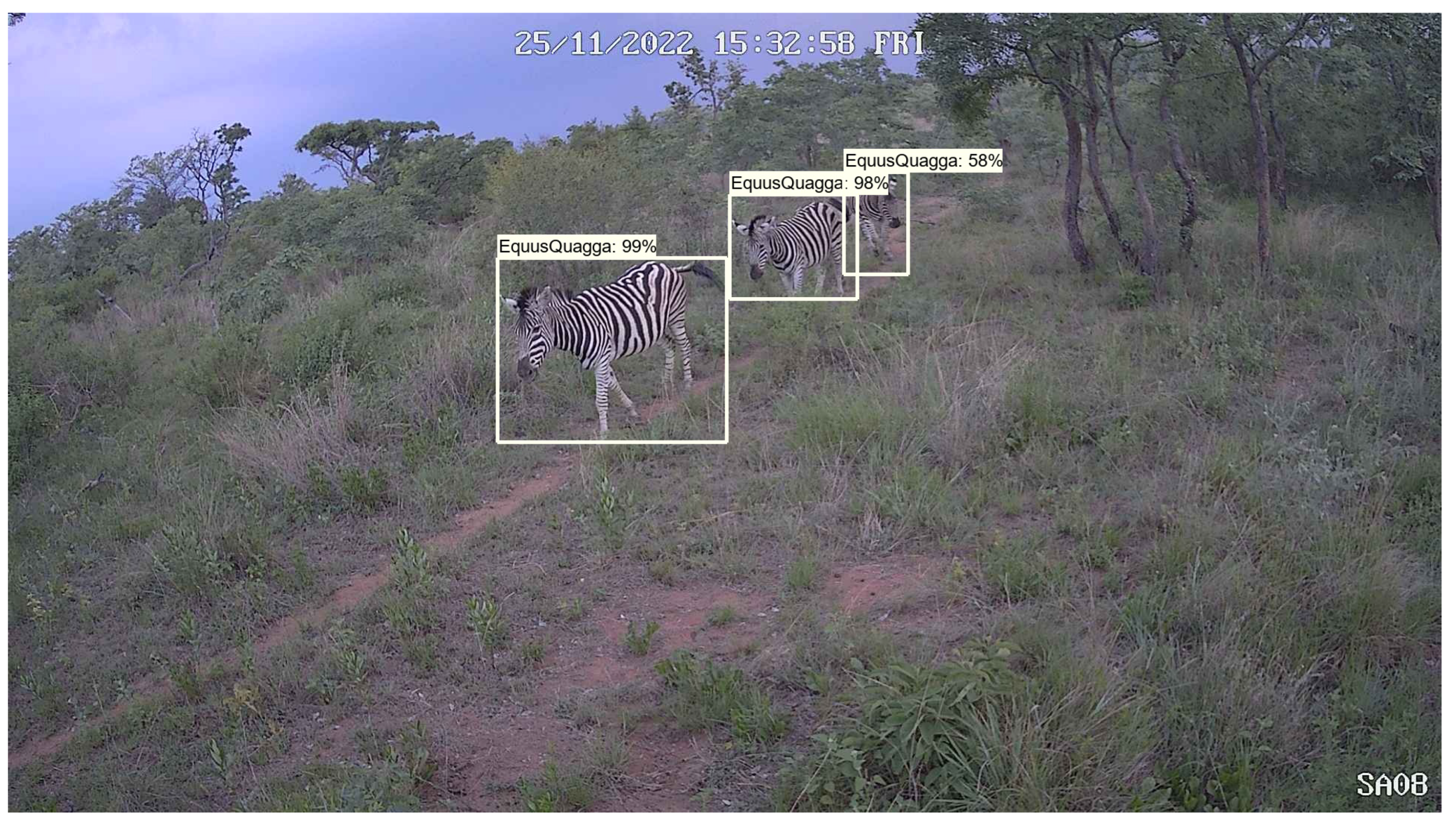
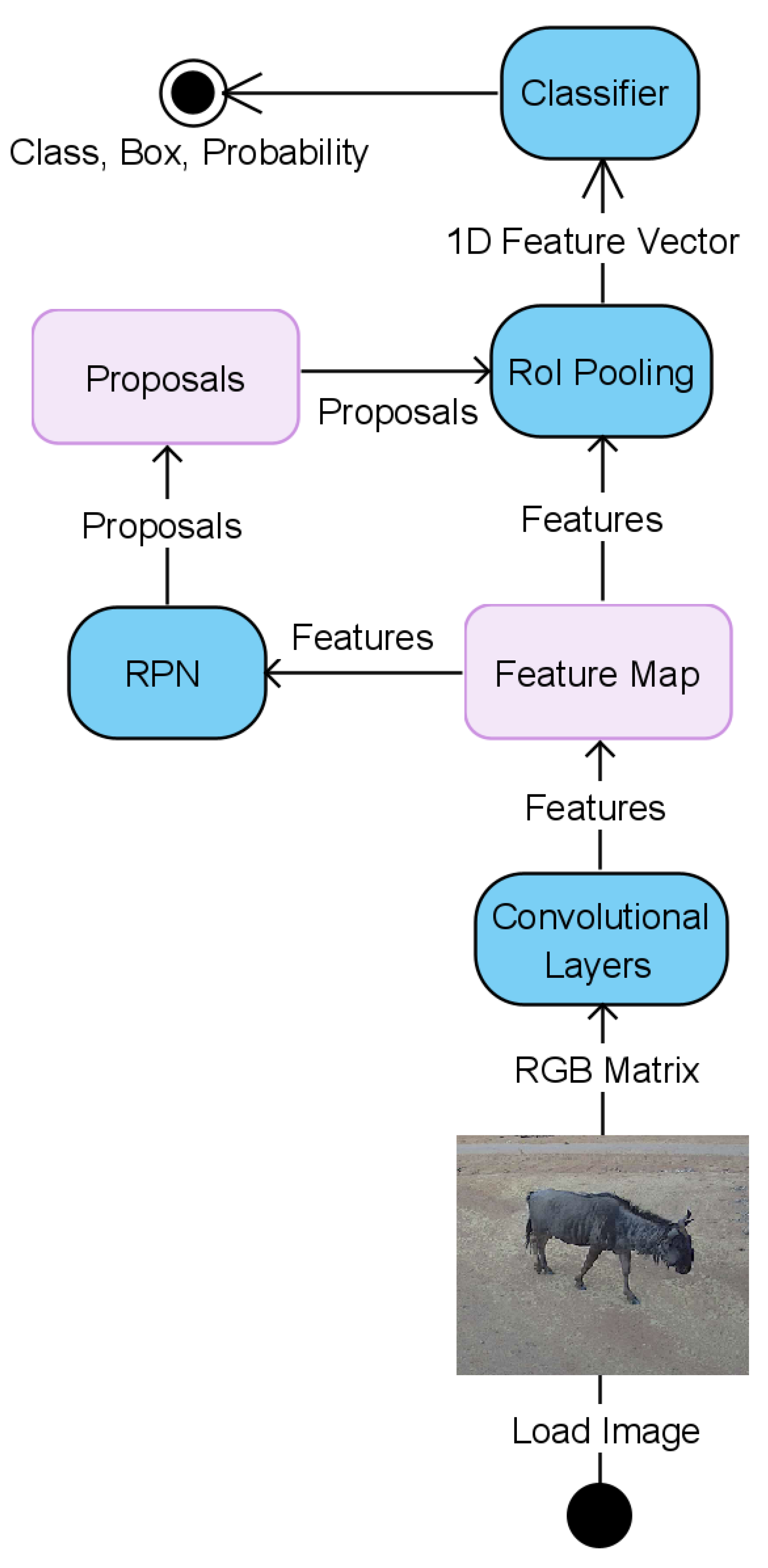
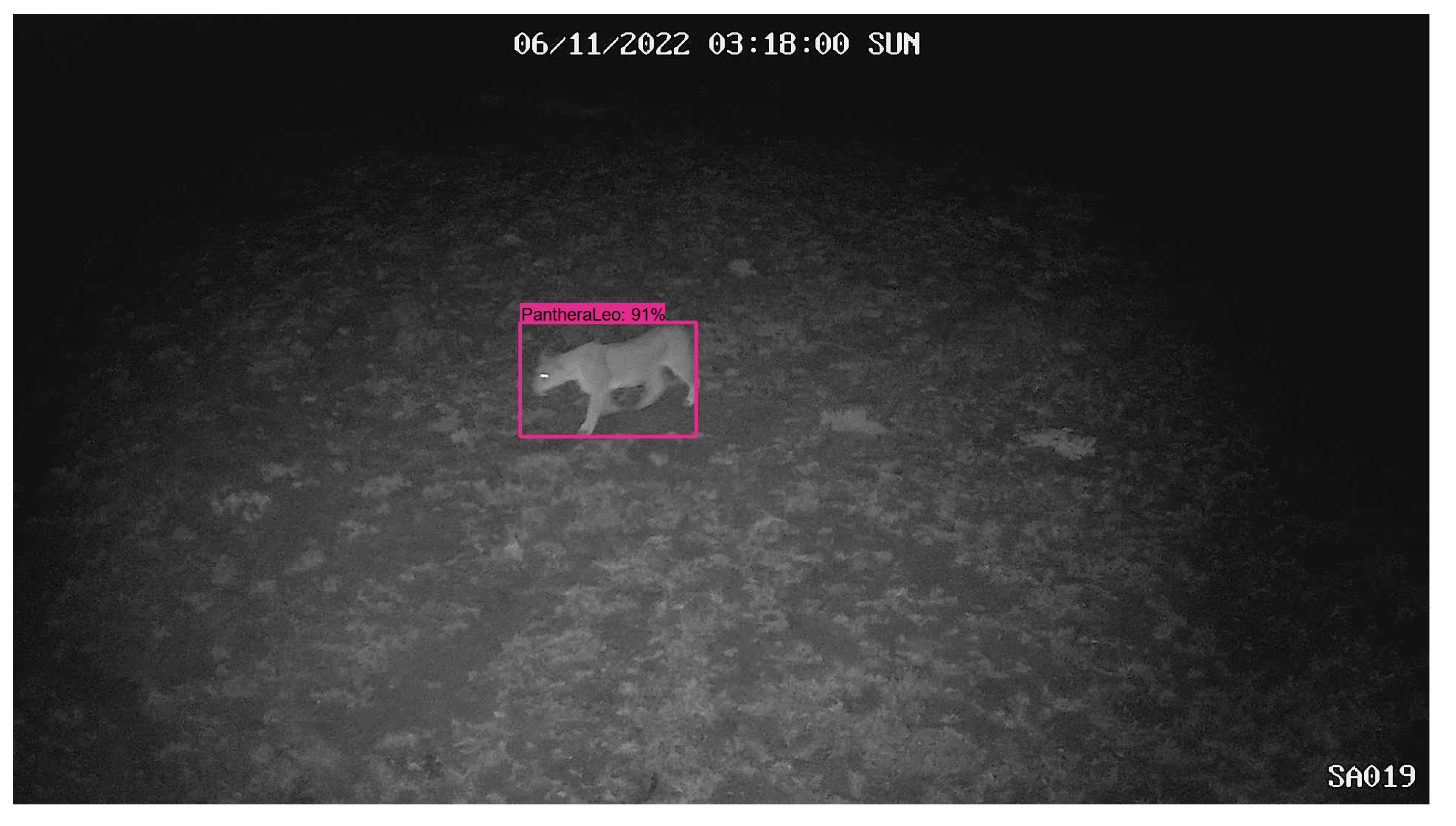
Figure 1 shows an example detection using our deep learning approach. In this example, three pence would be transferred from the species account to the guardian.
The remainder of this paper delves deeper into the key points discussed in the introduction. Section 2 provides a brief history of conservation, which serves as a foundation for the approach taken in this paper. Section 3 outlines the Materials and Methods used in the trial, which posits a new solution for addressing the challenges described. In Section 4, the results are presented before they are discussed in Section 5. Finally, Section 6 concludes the paper and provides suggestions for future work.

2. A Brief History of Conservation

Conservation is a multi-dimensional movement that involves political, environmental, and social efforts to manage and protect animals, plants, and natural habitats [38,39]. During the “Age of Discovery” in the 15th to 17th century [40], sport hunters in the US formed conservation groups to combat the massive loss of wildlife caused by European settlers [41]. As local policies emerged, people living close to areas where biodiversity was protected lost property, land, and hunting rights [42]. Settlers criminalised poaching, which was associated with local people who often hunted and fished for their survival [43]. Widespread laws led to the creation of protected areas and national parks [44], which were established within the context of colonial subjugation [45], economic deprivation [46], and systematic oppression of local communities [47].
As a result, local people engaged in “illegal” hunting to meet subsistence needs [48], earn income or status [49], pursue traditional practices of cultural significance [50], or address contemporary and historical injustices linked with conservation [49]. They viewed settlers (including sport hunters) as unwanted interlopers who stole their lands [43]. The industrial revolution in the 19th and early 20th centuries [51], marked by larger populations and working communities, further escalated the demand for natural resources, resulting in increased biodiversity loss [52,53]. Today, many local communities in ecologically unique and biodiversity-rich regions of the world still perceive conservation as a Western construct created by non-indigenous peoples who continue to exploit their lands and natural resources [54].
For decades, conservationists have debated whether it is human activity or climate change that has driven species extinctions and whether the loss of biodiversity is a recent phenomenon [3]. Studies have provided compelling evidence to show that it is, in fact, humans who are responsible for the wave of extinctions that have occurred since the Late Pleistocene, 126,000 years ago [55]. For example, toward the end of the Rancholabrean faunal age around 11,000 years ago, a substantial number of large mammals vanished from North America, which included woolly mammoths [56], giant armadillos [57], and three species of camel [58]. Similar extinctions were seen in New Zealand when the Dinornithiformes (Moa) became extinct about 600 years ago [59,60] and in Madagascar where the Archaeoindris fontoynontii (giant lemur) disappeared between 500 and 2000 years ago [61]. Many believe that species and population extinction is a natural phenomena [62], but the evidence suggests that human activity is accelerating species extinction and biodiversity loss [63].
Despite the efforts to protect biodiversity and natural habitats, we are sleepwalking ourselves into a sixth mass extinction [64]. Economic systems driven by limitless growth continue to negatively impact conservation efforts [65]. Rapid development and industrial expansion is depleting natural resources [66] and intensifying the conversion of large stretches of land for human use [67]. The Earth’s forests and oceans are persistently exploited by major corporations who view the planet’s natural resources as capital stock [68,69]. Economic models and financial markets treat natural systems as assets to be used immediately, leading to the abuse of nature for short-term profits with little regard for the long-term costs to society and the environment [70]. While The Economics of Ecosystems and Biodiversity (TEEB) attempt to hold large corporations to account [71], many believe we need nothing short of a redesign of corporations themselves if we are to successfully enable a transition to a ‘Green Economy’ [72]. Conservationists agree that biodiversity and natural systems are essential for human survival and economic prosperity but criticise the big corporations and political systems that prioritise immediate economic gains at the expense of the prosperity and well-being of both current and future generations [73].
The importance of involving local stakeholders as essential contributors in biodiversity monitoring and conservation efforts is emphasized in current perspectives [74]. Recognizing their role as capable natural resource managers, equitable schemes have been introduced to promote their engagement in locally grounded social impact assessments that consider the diverse implications of human activities in biodiversity-rich areas [75]. These efforts are largely driven by the Durban Accord led by the International Union for Conservation of Nature (IUCN) [76], which advocates for new governance approaches in protected areas to promote greater equity in local systems [77,78]. This necessitates a fresh and innovative strategy that upholds conservation objectives while inclusively integrating the interests of all stakeholders involved. This integrated approach aims to foster synergy between conservation, the preservation of life support systems, and sustainable development. While this paper does not claim to comprehensively address all the issues raised, it does offer a rudimentary tool that may help implement such a strategy by quantitatively accounting for biodiversity protection and equitable revenue sharing.

3. Materials and Methods

This section describes the implementation details for the digital stewardship and reward system posited in this paper that was deployed and evaluated in Welgevonden Game Reserve in Limpopo Province in South Africa. The section begins with a discussion on the training data collected for a Sub-Saharan Africa deep learning model, which was trained to detect 12 different animal species. A second dataset, which was used to evaluate the trained model, is also presented. This is followed by a discussion on the Faster R-CNN architecture [79] and its deployment in Conservation AI [80,81] to classify animals and validate the revenue-sharing scheme. The section is concluded with an overview of the performance metrics selected to evaluate the trained model and the inference tasks conducted during the trial.

3.1. Data Collection and Pre-Processing

The Sub-Saharan Africa model was trained with camera trap images of animals obtained from Conservation AI partners, which include Equus quagga, Giraffa camelopardalis, Canis mesomelas, Crocuta crocuta, Tragelaphus oryx, Connochaetes taurinus, Acinonyx jubatus, Loxodonta africana, Hystrix cristata, Papio sp., Panthera leo and 
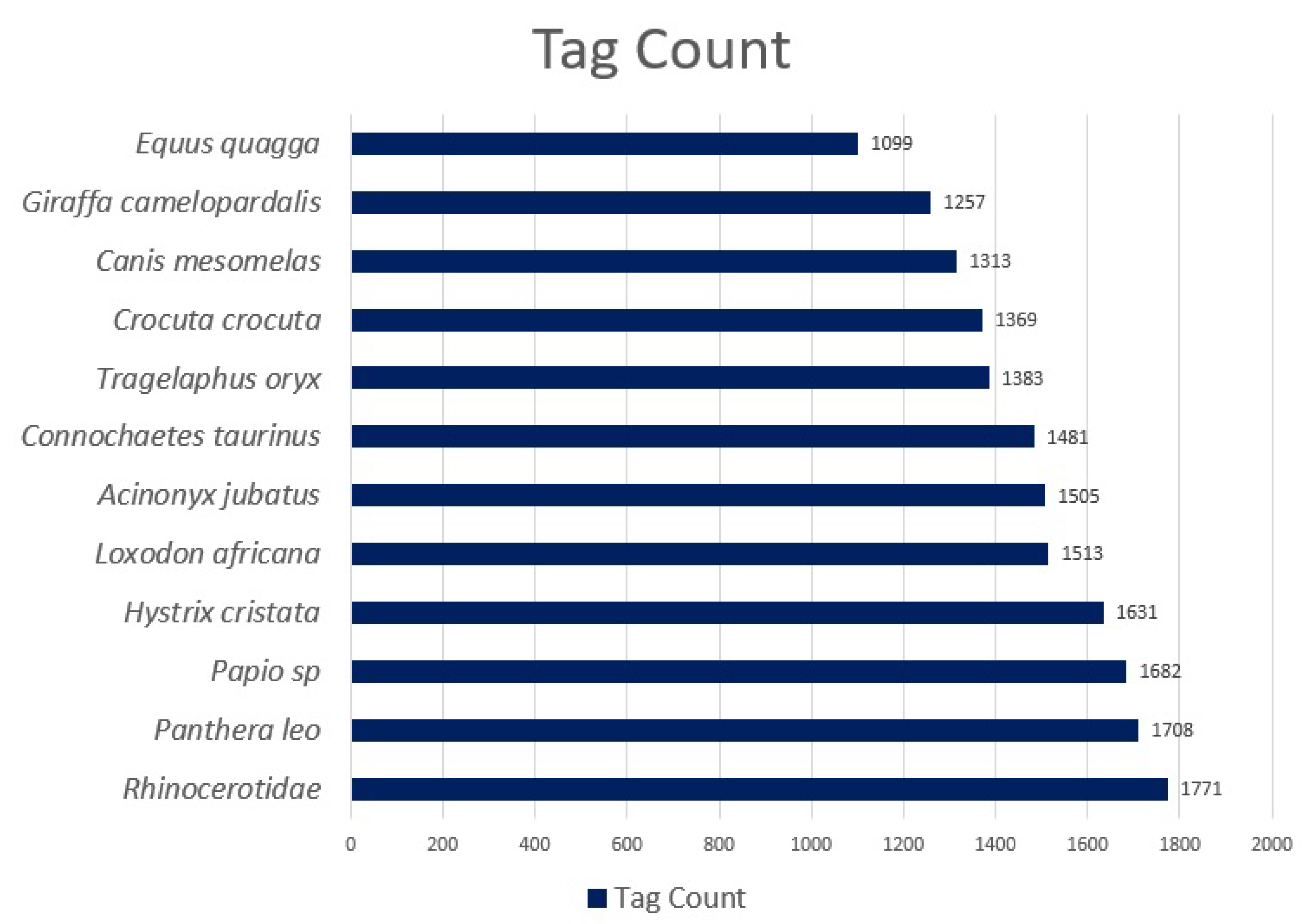
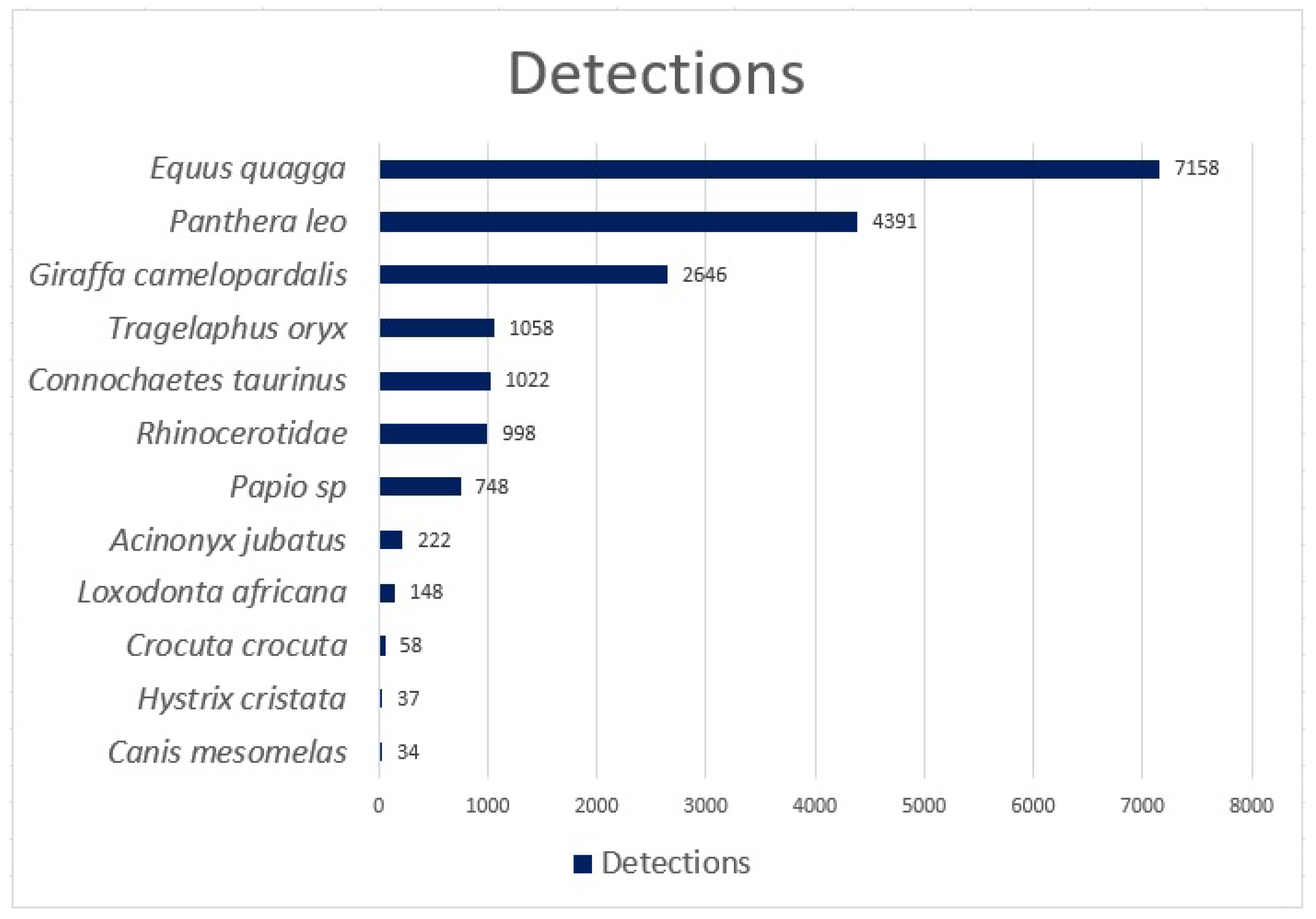
Rhinocerotidae, the 12 species considered in this study. The class distributions can be seen in Figure 2.
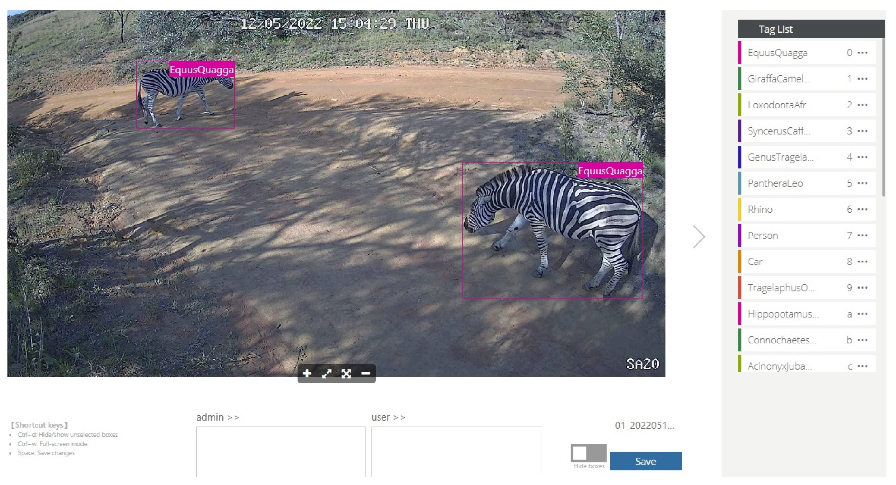
Following quality checks, between 1099 and 1771 tags per species were retained (17,712 in total). Tags are labelled binding boxes that mark the location of an object of interest (animal) within an image. Binding boxes were added to an image using the Conservation AI tagging website, which are serialised as coordinates in an XML file using the PASCAL VOC format [82]. The Conservation AI tagging site is shown in Figure 3.
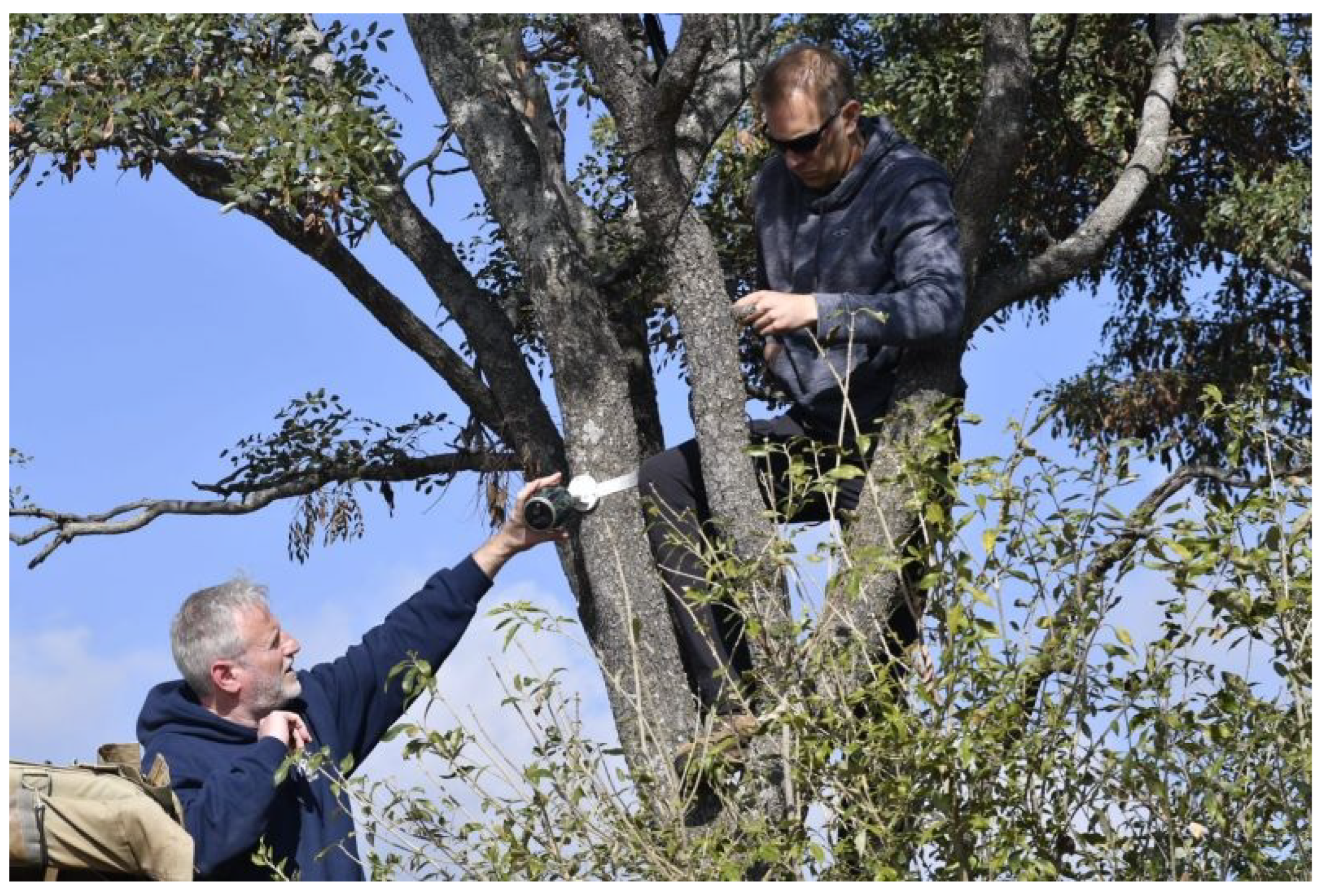
XML files are an intermediary representation used to generate TFRecords (a simple format for storing a sequence of binary records). Before the TFRecords were created, the tagged dataset was randomly split into a training set (90%—15,941 tags) and a validation set (10%—1771). Using the Tensorflow Object Detection API, the training and validation datasets were serialised into the two separate TFRecords and used to train the Sub-Saharan African model. The trained model was evaluated over the course of the trial with images obtained from 27 fixed Reolink Go 3/4G cameras installed in Weldgevonden Game Reserve in Limpopo Province in South Africa. Figure 4 shows an example of a camera being installed.
The camera resolution was configured to 1920 × 1072 pixels with a dots per inch (dpi) of 96. This configuration closely matches the aspect ratio resizer set in the pipeline.config used during the training of the Faster R-CNN. The Infrared (IR) trigger [83] was set at high sensitivity, and each camera was fitted with a camouflage sleeve and fastened to a tree once a connection to the Vodacom 3/4G network was established (an audible “Connection Succeeded” message is given). Each camera contained a rechargeable lithium-ion battery that was charged using a solar panel fastened to the tree and connected to the camera via a USB Type-B cable. The cameras had an IP65 waterproof rating, providing protection from low-pressure rainfall. Designed for security purposes, the cameras had a much wider aspect ratio than conventional camera traps, enabling the detection of animals at farther and wider distances. The installation process spanned seven days and covered an area of 400 km 2 (36,000 hectares). Camera sites were chosen along game paths, water sources, and grazing lawns. The cameras and solar panels were screwed into Burkea africana trees and out of reach of Loxodonta africana, which are known to destroy camera traps in the reserve.
The Reolink Go cameras were donated to us for the study by Reolink, and the 3/4G SIM cards were donated to us by Vodacom. The installed camera traps captured 12 different species over a ten-month period, which starting in May 2022 and ending in February 2023. During the trial period, 18,520 detections were made, and 19,380 blanks were reported, totalling 37,900 images. Figure 5 summarises the number of species identified during the trial.
The 37,900 images were used to generate ten subsets of the data to make the evaluation more achievable. A 5% margin of error and a confidence level of 95% in each dataset was maintained using 29 images from each of the 12 animal classes and 29 randomly selected images from the blanks (each of the 10 datasets contained 377 images). The evaluation metrics were calculated for each of the 10 datasets and averaged to produce a final set of metrics for the model. This is a common approach used in object detection, which provides a more comprehensive understanding of the performance of and object detection model because it:
  • Increases diversity. Object detection models perform differently on different datasets due to variation in object types, sizes, orientations, and backgrounds. Using multiple datasets increases the diversity of the data, which allows the model to be evaluated using a wide range of scenarios.
  • Ensures robustness. Models that perform well on a single dataset may not necessarily generalise well to new datasets. Evaluating the model on multiple datasets and averaging the results assesses the robustness and ability to perform consistently across different datasets.
  • Provides a fair comparison. Comparing the performance of different object detection models is important to evaluate them on the same datasets to ensure a fair comparison. Using multiple datasets and averaging the results reduces the impact of dataset bias and allows a more reliable estimate of the model’s true performance to be obtained.
  • Gives more representative results. Object detection evaluation metrics, such as mAP, can be sensitive to small variations in detection results. By averaging the results across multiple datasets, we can obtain more representative and stable evaluation metrics that reflect the model’s overall performance.

3.2. Faster R-CNN

The Faster R-CNN architecture was trained to detect and classify 12 animal species [79]. The architecture comprises three components: (a) a convolutional neural network (CNN) [84] that generates feature maps [85] and performs classification, (b) a region proposal network (RPN) [79] that generates regions of interest (RoI), and (c) a regressor that locates each object in the image and assigns a class label. Figure 6 shows the Faster R-CNN architecture.
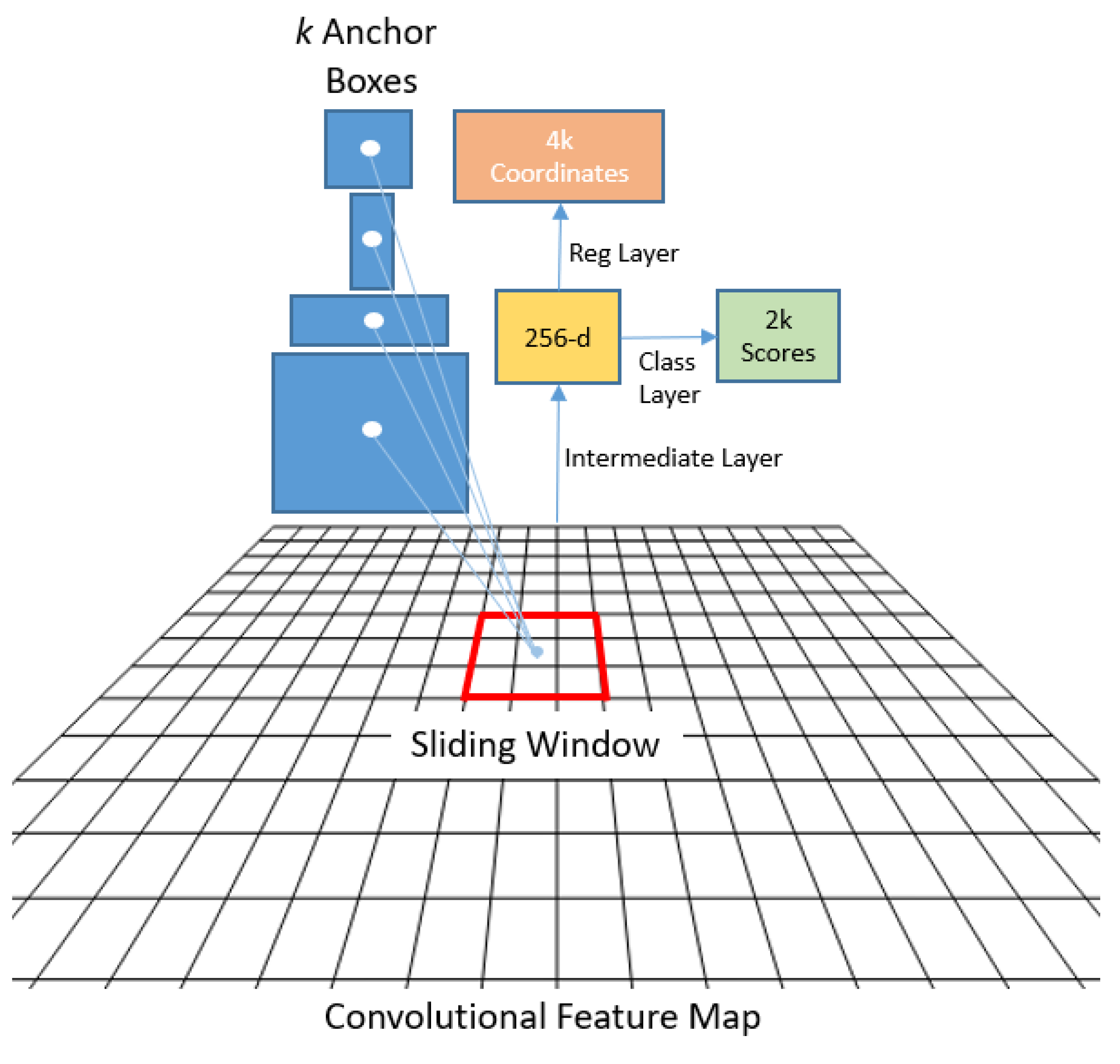
The RPN is a crucial component in the Sub-Saharan Africa model, as it identifies potential animal species in camera trap images by leveraging the features learned in the base network (ResNet101 in this case [86]). Unlike early R-CNN networks [87], which relied on a selective search approach [88] to generate region proposals at the pixel level, the RPN operates at the feature map level, generating bounding boxes of different sizes and aspect ratios throughout the image, as depicted in Figure 7.
The RPN achieves this by employing anchors or fixed bounding boxes, represented by 9 distinct size and aspect ratio configurations, to predict object locations. It is implemented as a CNN, with the feature map supplied by the base network. For each point in the image, a set of anchors is generated, with the feature map dimensions remaining consistent with those of the original image.
The RPN produces two outputs for each anchor bounding box: a probability objectness score and a set of bounding box coordinates. The first output is a binary classification that indicates whether the anchor box contains an object or not, while the second provides a bounding box regression adjustment. During the training process, each anchor is classified as belonging to either a foreground or background category. Foreground anchors are those that have an intersection over union (IoU) greater than 0.5 with the ground-truth object, while background anchors are those that do not. The IoU is defined as the ratio of the intersection to the union of the anchor box and the ground-truth box. To create mini-batches, 256 balanced foreground and background anchors are randomly sampled, and each batch is used to calculate the classification loss using binary cross-entropy. If there are no foreground anchors in a mini-batch, those with the highest IoU overlap with the ground-truth objects are selected as foreground anchors to ensure that the network learns from samples and targets. Additionally, anchors marked as foreground in the mini-batch are used to calculate the regression loss and transform the anchor into the object. The IoU is defined as:
IoU = Anchor box Ground Truth box Anchor box Ground Truth box
Since anchors can overlap, proposals may also overlap on the same object. To address this, non-maximum suppression (NMS) is performed to eliminate intersecting anchor boxes with lower IoU values [89]. An IoU greater than 0.7 is indicative of positive object detection, while values less than 0.3 describe background objects. It is important to exercise caution while setting the IoU threshold as setting it too low may lead to missed proposals for objects, while setting it too high may result in too many proposals for the same object. Typically, an IoU threshold of 0.6 is sufficient. Once NMS is applied, the top N proposals sorted by score are selected.
The loss functions for both the classifier and bounding box calculation are defined as:
L c l s ( p i , p i * ) = ( p i * l o g ( p i ) + ( 1 p i * ) l o g ( 1 p i ) )
L r e g ( t i , t i * ) = Σ i { x , y , w , h } s m o o t h L 1 ( t i t i * )
where
s m o o t h L 1 ( t i t i * ) = 0.5 x 2 i f | t i t i * | < 1 | x | 0.5 o t h e r
where p i is the object possibility, t i is the 4 k anchor coordinate, p i * is the ground-truth label, t * is the ground-truth coordinate, L c l s is the classification loss (log loss), and L r e g is the regression loss (smooth L1 loss).
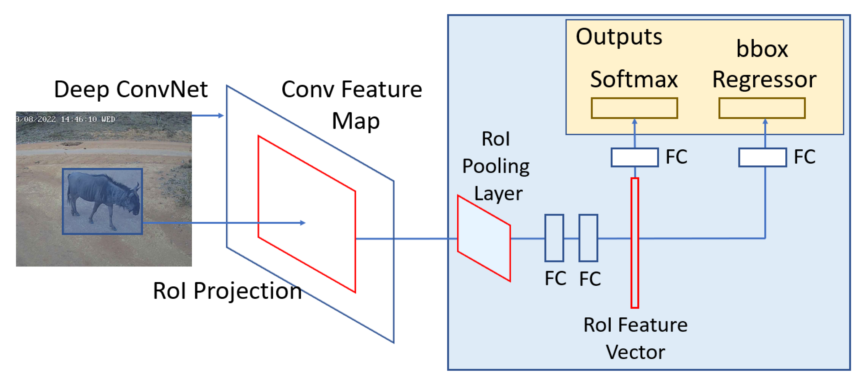
After generating object proposals in the RPN step, the next task is to classify and assign a category to each bounding box. In the Faster R-CNN framework, this is accomplished by cropping the convolutional feature map using each proposal and then resizing the crops to 14 × 14 × convdepth using interpolation. To obtain a final 7 × 7 × 512 feature map for each proposal via RoI pooling, max pooling with a 2 × 2 kernel is applied after cropping. These default dimensions are set by the Faster R-CNN [87] but can be customised depending on the specific use case for the second stage.
The Faster R-CNN architecture takes the 7 × 7 × 512 feature map for each proposal, flattens it into a one-dimensional vector, and passes the vector through two fully connected layers of size 4096 with rectifier linear unit (ReLU) activation [90]. To classify the object category, an additional fully connected layer is implemented with N + 1 units, where N is the total number of classes and the extra unit corresponds to background objects. Simultaneously, a second fully connected layer with 4N units is implemented for predicting the bounding box regression parameters. These 4 parameters are Δ c e n t e r x , Δ c e n t e r y , Δ w i d t h , and Δ h e i g h t for each of the N possible classes. The Faster R-CNN architecture is illustrated in Figure 8.
Targets in the Faster R-CNN are computed in a similar way to RPN targets but with different classes taken into account. Proposals with an IoU greater than 0.5 with any ground-truth box are assigned to that ground truth. Proposals with an IoU between 0.1 and 0.5 are designated as background, while proposals with no intersection are ignored. Targets for bounding box regression are computed for proposals that have been assigned a class based on the IoU threshold by determining the offset between the proposal and its corresponding ground-truth box. The Faster R-CNN is trained using backpropagation [91] and stochastic gradient descent [92]. The loss function in the Faster R-CNN is calculated as follows:
L ( p , u , t u , v ) = L c l s ( p , u ) + λ . [ u 1 ] L r e g ( t u , ν )
where p represents the object probability, u represents the predicted classification class, t represents the ground-truth label, and v represents the ground-truth coordinates for class u. Specifically, the classification loss function L c l s is given by:
L c l s ( p , u ) = log ( e p u Σ j = 1 K e p j )
where p is the object possibility, u is the classification class, and K is the total number of classes. L r e g for bounding box regression can be calculated using the equation described in (3), with t u and v as input.
To refine the object detection, the Faster R-CNN applies a bounding box adjustment step, which considers the class with the highest probability for each proposal. Proposals assigned to the background class are ignored. Once the final set of objects have been determined, based on the class probabilities, NMS is applied to filter out overlapping boxes. A probability threshold is also set to ensure that only highly confident detections are returned, thereby minimising false positives.
For the complete Faster R-CNN model, there are two losses for the RPN and two for the R-CNN. The four losses are combined through a weighted sum, which can be adjusted to give the classification losses more prominence than the regression losses or to give the R-CNN losses more influence over the RPNs.

3.3. Transfer Learning

The Faster R-CNN model was fine-tuned in this study using the dataset containing 12 animal classes; this is known as transfer learning [93]. This crucial technique combats overfitting [94], which is a common problem in deep learning when training with limited data. The base model used was ResNet101, a residual neural network [86] that was pre-trained on the COCO dataset consisting of 330,000 images and 1.5 million object instances [82]. Residual neural networks employ a highway network architecture [95], which enables efficient training in deep neural networks using skip connections to mitigate the issue of vanishing or exploding gradients.

3.4. Model Training

The model training process was performed on a 3U blade server featuring a 24 Core AMD EPYC7352 CPU processor, 512GB RAM, and 8 Nvidia Quadro RTX8000 graphics cards totalling 384GB of GPU memory [96]. To create the training pipeline, we leveraged TensorFlow 2.5 [97], the TensorFlow Object Detection API [98], CUDA 10.2, and CuDNN version 7.6. The TensorFlow configuration file was customised with several hyperparameters to optimise the training process:
  • Setting the minimum and maximum coefficients for the aspect ratio resizer to 1024 × 1024 pixels, respectively, to minimise the scaling effect on the data.
  • Retraining the default feature extractor coefficient to provide a standard 16-pixel stride length, which helps maintain a high-resolution aspect ratio and improve training time.
  • Setting the batch size coefficient to sixty-four to ensure that the GPU memory limits are not exceeded.
  • Setting the learning rate to 0.0004 to prevent large variations in response to the error.
In order to improve generalisation and to account for variance in the camera trap images, the following augmentation settings were used:
  • Random_adjust_hue, which adjusts the hue of an image using a random factor.
  • Random_adjust_contrast, which adjusts the contrast of an image by a random factor.
  • Random_adjust_saturation, which adjusts the saturation of an image by a random factor.
  • Random_square_crop_by_scale, which was set with a s c a l e _ m i n of 0.6 and a s c a l e _ m a x of 1.3.
ResNet101 employs the Adam optimiser to minimise the loss function [99]. Unlike optimisers that rely on a single learning rate (alpha) throughout the training process, such as stochastic gradient descent [100], Adam uses the moving averages of the gradients m t and squared gradients v t , along with the parameters beta1/beta2, to dynamically adjust the learning rate. Adam is defined as:
m t = β 1 m t 1 + ( 1 β 1 ) g t v t = β 2 v t 1 + ( 1 β 2 ) g t 2
where m t and v t are estimates of the first and second moment of the gradients. Both m t and v t are initialised with 0 s. Biases are corrected by computing the first and second moment estimates:
m ^ t = m t 1 β 1 t v ^ t = v t 1 β 2 t
Parameters are updated using the Adam update rule:
θ t + 1 = θ t n v ^ t + ϵ m ^ t ·
To overcome the problem of saturation changes around the mid-point of their input, which is common with sigmoid or hyperbolic tangent (tanh) activations [101], the ReLU activation function is adopted [102]. ReLU is defined as:
g ( x ) = m a x ( 0 , x )

3.5. Inference Pipeline

The Sub-Saharan Africa model was hosted on a Nvidia Triton Inference Server (version 22.08) on a custom-built machine with an Intel Xeon E5-1630v3 CPU, 256GB of RAM, and an Nvidia Tesla T4 GPU [103]. The real-time cameras transmitted images over 3/4G communications every time the IR sensor was triggered. The trigger distance was set to “High”, which supports a 9 m (30 feet) trigger range [36]. Images were received from cameras using the Simple Mail Transfer Protocol (SMTP) [104] and submitted to the Sub-Saharan Africa model using a RestAPI [105]. All data were stored in a MySQL database (images are stored in local directories; the MySQL database contains hyperlinks to all images with detections).

3.6. BioPay

BioPay is a RestAPI service provided by Conservation AI (this is not a public facing service but an experimental module for research purposes only; see Figure 9).
The service transferred funds between individual species accounts and a guardian account each time a camera was trigged and an associated animal was detected (see Figure 1 and Figure 10, Figure 11 and Figure 12 for sample detections). To ensure efficient fund management, 12 separate makeshift bank accounts, each dedicated to a distinct species, and a central guardian makeshift account were created using the PayPal Sandbox Developer SDKs [106]. Upon successful classification of an animal, 0.1 GBP was securely transferred from the corresponding species account to the guardian account. Each account was credited with GBP 100 at the start of the trial.

3.7. Evaluation Metrics

RPNLoss/objectiveness, RPNLoss/localisation, BoxClassifierLoss/classification, BoxClassifierLoss/localisation, and TotalLoss are used to evaluate the model during training [97,107]. RPNLoss/objectiveness evaluates the model’s ability to generate bounding boxes and classify background and foreground objects. RPNLoss/localisation measures the precision of the RPN’s bounding box regressor coordinates for foreground objects, which is to say, how closely each anchor target is to the nearest bounding box. BoxClassifierLoss/classification measures the output layer/final classifier loss for prediction, and BoxClassifierLoss/localisation measures the bounding box regressor’s performance in terms of localisation. TotalLoss combines all the losses to provide a comprehensive measure of the model’s performance.
The validation set during training was evaluated using mAP (mean average precision), which serves as a standard measure for assessing object detection models. mAP is defined as:
m A P = q = 1 Q A v e P ( q ) Q
where Q is the number of queries in the set and A v e P ( q ) is the average precision ( A P ) for a given query a.
mAP was computed for the binding box locations using the final two checkpoints. The calculation involves measuring the percentage IoU between the predicted bounding box and the ground-truth bounding box and is expressed as:
I o U = A r e a o f O v e r l a p A r e a o f U n i o n
The detection accuracy and localisation accuracy were measured using two distinct IoU thresholds, namely @.50 and @.75, respectively. The @.50 threshold evaluates the overall detection accuracy, and the higher @.75 threshold focuses on the model’s ability to accurately localise objects.
Accuracy, precision, sensitivity, specificity, and F1-score were used to evaluate the performance of the trained model during inference, in other words, using the image data collected during the trial. Accuracy is defined as:
A c c u r a c y = T P + T N T P + F P + T N + F N
where TP is true positives, TN is true negatives, FP is false positives, and FN is false negatives. The accuracy metric provides an overall assessment of the object detection model’s ability to make inferences on unseen data. This metric is often interpreted alongside the other metrics defined below.
Precision was used to assess the model’s ability to make true-positive detections and is defined as:
P r e c i s i o n = T P T P + F P
It measures the fraction of true-positive detections out of all detections made by the trained model. In object detection, a true-positive detection occurs when the model correctly identifies an object and predicts its location in the image. A high precision indicates that the model has a low rate of false positives, meaning that when it makes a positive detection, it is highly likely to be correct.
Sensitivity, also known as recall, measures the proportion of true positives correctly identified by the trained model during inference. In other words, it measures the model’s ability to detect all positive instances in the dataset. A high sensitivity indicates that the model has a low rate of false negatives, meaning that when an object is present in the image, the model is highly likely to detect it. This metric is defined as:
S e n s i t i v i t y = T P T P + F N
Specificity measures the proportion of true-negative detections that are correctly identified by the model. In object detection, true-negative detections refer to areas of an image where there is no object of interest. In this paper, we evaluate blank images to satisfy this metric, as it is important to ensure that classifications are based on features extracted from animals and not the background. Specificity is defined as:
S p e c i f i c i t y = T N T N + F P
Finally, the F1-score combines precision and recall into a single score. A high F1-score indicates that the model has both high precision and high recall, meaning that it can accurately identify and localise objects in the image. F1-score is defined as:
F 1 S c o r e = 2 P r e c i s i o n S e n s i t i v i t y ( R e c a l l ) P r e c i s i o n + S e n s i v i t i t y ( R e c a l l )
The ground truths for the 10 subsampled datasets were provided by conservationists and biologists who appear as co-authors in the paper. The ground truths were used to calculate the detections generated by the in-trial model.

4. Evaluation

The results obtained during the training of the Sub-Saharan Africa model are presented first. The model is then evaluated in a real-world setting to assesses its ability to classify animal species in images captured during the trial. This section is concluded with the results obtained for the financial transactions taken between animals and the guardian bank account when positive detections are made.

4.1. Training Results for the Sub-Saharan Model

In the first evaluation, the training set (containing 17,712 images; see Figure 2 for species tag distributions) was used to fit the model. The dataset was randomly split, as previously discussed in Section 3.1, and trained over 28,000 steps (438 epochs) using a batch size of 64.

4.1.1. RPN and Box Classification Results for the Training Dataset

The outcomes depicted in Table 1 indicate that the model is capable of detecting candidate regions of interest with sufficient accuracy (loss = 0.0366). The RPN can effectively model localisation (loss = 0.0112). Classification loss (loss = 0.1833) is higher than previous losses, which shows the model is less precise at classifying objects of interest than locating them. Box classifier localisation (loss = 0.0261) is comparable to the RPN results and confirms that the model can sufficiently identify candidate bounding boxes. The total loss value (0.2244) combines both the RPN and box classification losses and indicates that the model’s predictions are relatively close to the ground-truth labels. In most cases, a total loss = 0.2244 in object detection is considered a good outcome.

4.1.2. RPN and Box Classification Results for the Validation Dataset

Table 2 provides the results for the validation set, which are generally consistent with those produced by the training set. The loss for regions of interest (loss = 0.0530) is marginally higher but not significantly higher. The same applies to RPN localisation (loss = 0.0384), which is also slightly higher but not significantly higher. Both the losses for classification and box classifier localisation, 0.1533 and 0.0242, respectively, are similar to those in Table 1. The combined losses indicate that the validation set produces good results, as shown in total loss (loss = 0.2690) in Table 2. It is worth noting that the training and validation metrics are close, meaning there was no evidence of overfitting during model training.

4.1.3. Precision and Recall Results for Validation Dataset

The mAP values in Table 3 provide the mean of the average precisions achieved for all classes using IoU thresholds between 0.5 and 0.95 with 0.05 increments. The result (mAP = 0.7542) indicates that 24.8% false positives were observed across all classes and IoU thresholds. An mAP of 0.7542 would generally indicate that the model is able to correctly detect objects with a high level of accuracy. According to the precision metrics for objects of different sizes, the model appears to be more proficient at detecting larger-sized objects (0.7815) within images, as opposed to medium and smaller objects (0.3528 and 0.1362 respectively). An mAP of 0.9449 and 0.8601 at IoU thresholds of 0.50 and 0.75, respectively, indicate that the model is able to accurately detect objects with a high level of precision across a wide range of IoU thresholds.
The recall values in Table 4 indicate that the model can retrieve 62.39% of all images among the top 1 images retrieved (Recall/AR@1). As the number of returned images increases, the number of relevant images increases (Recall/AR@10 = 0.8060 and Recall/AR@100 = 0.8140). In object detection, these are again satisfactory results. The recall values for AR@100 (small, medium, and large) show that the model is better at detecting large and medium objects in images (0.8496 and 0.5079, respectively) as opposed to smaller objects (0.3344).

4.2. Trial Results Using the Sub-Saharan African Model

The trained model was deployed and used in the Welgevonden Game Reserve in Limpopo Province in South Africa to detect 12 animal species captured in camera traps. During the ten-month trial, 18,520 images with detections were recorded, and there were 19,380 images with no animal in them (blanks). In total, 37,800 images were collected. Figure 5 shows the distribution of all animal detections. Due to the size of the dataset, 10 subsets of the data were created to make the evaluation achievable.

4.2.1. Performance Metrics for Inference

The results in Table 5 show that the model achieves high accuracy scores for all animal classes, with values between 98.70% and 100.00%. The model’s precision scores are more varied, with scores between 60.00% and 100.00%, with the Acinonyx jubatus and Panthera leo classes having the lowest values. Overall, the average model precision (87.14%) is considered a good result in object detection. However, there are issues with several classes (Hystrix cristata, Acinonyx jubatus and Panthera leo) that require further investigation. Sensitivity is consistently high for all classes, indicating that the model correctly identifies positive samples. Again, the overall sensitivity for the model (96.38%) is high, which shows that a large proportion of actual positive cases are correctly identified by the model. The classes with the lowest sensitivity values (Tragelaphus oryx and Panthera leo, with 90.90% and 90%, respectively) may need further investigation. This seems to be because the model is heavily reliant on the colour and shape of the Tragelaphus oryx. Specificity is consistently high across all classes. Again, the overall specificity for the model is high (99.62%), which indicates the model can effectively detect negative cases (i.e., distinguish between blank images and animal classes). Finally, the F1-scores provide the harmonic mean for precision and recall (sensitivity), and most classes are generally high. The overall model F1-score (90.33%) is good, although addressing issues around precision for the classes mentioned above will improve the F1-score.

4.2.2. Confusion Matrix

Examining the confusion matrix in Table 6, the results align with those in Table 5. The model accurately predicted all samples for the Canis mesomelas, Hystrix cristata, Acinonyx jubatus, and Panthera leo classes. Additionally, the model performed remarkably well for the Loxodonta africana, Papio sp., and Blank classes, with only a few misclassifications. However, the model misclassified 42 samples from the Connochaetes taurinus class as Tragelaphus oryx and 17 samples as Loxodonta africana. Similarly, for the Tragelaphus oryx class, the model misclassified 15 samples as Equus quagga and 11 samples as Connochaetes taurinus. This information highlights the specific areas where future re-training is required.

4.2.3. ROC and AUC for Sub-Saharan Classification Model

The ROC in Figure 9 provides a visual assessment of the model’s inference results, which indicates the model performed remarkably well for all animal classes, as the AUC values are high. It can be concluded that the trained model in this trial achieved excellent results for each class. The plot and AUC values align with the outcomes presented in Table 5 and Table 6, which validates the deep learning aspects presented in this paper.

4.2.4. BioPay

The evaluation is concluded with the outcomes obtained from the BioPay service. Table 7 shows the ordered species detection counts collected during the ten-month trial. The Canis mesomelas species had the lowest count with only 34 detections, whereas the Equus quagga had the highest at 7158. During the trial, each detected animal initiated the transfer of GBP 0.1 from the respective species account to the guardian account. Following the trial’s completion, the guardian earned GBP 0.34 for the Canis mesomelas, GBP 0.37 for the Hystrix cristata, GBP 0.58 for the Crocuta crocuta, GBP 1.48 for the Loxodonta africana, GBP 2.22 for the Acinonyx jubatus, GBP 7.48 for the Papio sp., GBP 9.98 for the Rhinocerotidae, GBP 10.22 for the Connochaetes taurinus, GBP 10.58 for the Tragelaphus oryx, GBP 26.46 for the Giraffa camelopardalis, GBP 43.91 for the Panthera leo, and GBP 71.58 for the Equus quagga. The guardian’s total earnings for the ten-month trial was GBP 185.20.

5. Discussion

Using deep learning for species identification and 3/4G camera traps for capturing images of animals, we successfully deployed a Sub-Saharan Africa model capable of detecting 12 distinct animal species. The deep learning model was trained with 1099 and 1771 tags per animal, which enabled us to effectively monitor a 400 km 2 region in Welgevonden Game Reserve in Limpopo Province in South Africa using 27 real-time 3/4G camera traps for a period of 10 months. During the model training phase, it was possible to obtain good results for the RPN (objectness loss = 0.0366 and localisation loss = 0.0112 for the training set; objectness loss = 0.0530 and localisation loss = 0.0384 for the validation set). The box classifier losses for classification and localisation were also good (classification loss = 0.1833 and localisation loss = 0.0261 for the training set; classification loss = 0.1533 and localisation loss = 0.0242 for the validation set). Combining the evaluation metrics, it was possible to obtain a total loss = 0.2244 for the training set and a total loss = 0.2690 for the validation set. Again, these are good results for an object detection model. The precision and recall results obtained for the validation set were also good, with mAP = 0.7542, [email protected] = 0.9449, [email protected] = 0.8601, AR@1 = 0.6239, AR@100 = 0.8140, and AR@100(Large) = 0.8357. The results show that the model can accurately identify objects in images with high precision and recall while maintaining a high level of localisation accuracy.
Throughout the ten-month trial, the sensitivity (96.38%), specificity (99.6%), precision (87.14%), F1-score (90.33%), and sccuracy (99.31%) metrics were consistently high for most species, thereby confirming the training results. However, the precision scores for Hystrix cristata and Acinonyx jubatus were lower, with 77.09% and 59.33%, respectively. Figure 10 shows a sample image of a Hystrix cristata and indicates that they appear as small objects in the image, which aligns with the model’s limited ability to detect small objects, as evidenced in Table 3 and Table 4. Similarly, Figure 11 shows a sample image of Acinonyx jubatus, which is also small, thereby making their detection more challenging, especially at night when the quality of images is lower. It is also worth noting that the model was trained using traditional camera trap data. Historically, conservationists have fixed camera traps much lower down (closer to the ground) so the animal appears larger in the image. As can be seen in Figure 4, our camera trap deployments are much higher. This was done to prevent the cameras and solar panels being damaged by passing wildlife. Obviously, having cameras lower down removes issues where far-away animals are misclassified, as they would not be in the image. Camera deployment needs some further consideration.
The Canis mesomelas, Crocuta crocuta, and Loxodonta africana were also found to be misclassified as Acinonyx jubatus, Rhinocerotidae, and either Rhinocerotidae or Panthera leo, respectively, as evidenced in the confusion matrix in Table 6. Hystrix cristata was never misclassified, but Equus quagga and Rhinocerotidae were mistakenly classified as Hystrix cristata. Papio sp. was misclassified as either Crocuta crocuta or Acinonyx jubatus. Although Rhinocerotidae performed well, it was also mistakenly classified as Loxodonta africana or Panthera leo, along with Hystrix cristata. Tragelaphus oryx and Connochaetes taurinus were occasionally misclassified as each other. Giraffa camelopardalis was identified correctly, and Panthera leo was always correctly identified. Equus quagga also performed well, but low-quality images captured at night sometimes resulted in them being misclassified as another species. To address this issue, the Sub-Saharan Africa model was continuously trained, and many of the incorrect classifications encountered during the trial were identified and incorporated back into the training dataset to improve model performance. The version of the model used during the trial was version 18, while the current version is 22.
Distance was also a problem in the study [108]. Animals closest to the camera, as one would expect, classify much better than those farther away. In the trial, the camera trigger distance was set to “High”, which allows objects to be detected up to 30 feet away (9 m). Again, this configuration is not typical in traditional camera trap deployments. Obviously, detections farther away depend on the size of the animal. Detecting large animals, such as a Loxodonta africana or a Giraffa camelopardalis, is mostly successful, while detecting smaller animals, such as a Papio sp., is less so, or at least the confidence scores are significantly lower. This can be seen in Figure 13, where the Panthera leo has a lower confidence score than animals captured up close, as shown in Figure 1, where Equus quaggas captured close up have a higher confidence score than those in the distance. Not having a distance protocol in the study impacted the inclusion criteria for evaluation. We evaluated farther detections that would not normally trigger the camera trap (animals closer to the camera were responsible for the trigger), and this likely impacted the results in some instances. Further investigation is needed to define a protocol to map distance and detection success and incorporate it into the ground-truth object selection criteria for evaluation.
The BioPay service performed as expected, and the results show the successful transfer of funds between animals and the associated guardian. The detection results during inference show that overall detection success was high, with a small number of misclassifications. This means that money would be transferred from a species account when in fact that animal was not actually seen. This will always be a difficult challenge to address, but a small margin of error in this case is negligible. Obviously, this may not be the case when species are appropriately valued where highly prized animals could transfer large amounts of money when they are misclassified. This will need to be considered in future studies. Any BioPay system would need to be highly regulated, and guardians would have the right to raise concerns and appeal any decisions made. For example, a guardian might claim they have seen an animal, but it was not classified by the system. In this instance, the guardian would have the chance to present their evidence and dispute the outcome, much as individuals do in any other type of financial system. Depending on the outcome, the guardian would be paid or the claim would be dismissed.
Another important point to raise is the incentive surrounding the monetary gain guardians would receive for caring for animals compared to the amount obtained for poaching. Obviously, the former would have to be much higher if something such as BioPay is to be given a chance of success. In other words, receiving £100 pounds a month to ensure the safety of a Rhinocerotidae compared to the few thousand pounds they would receive for its horn (poachers lower down the IWT chain receive significantly less than those close to the source of the sale [109]) would unlikely be attractive to those involved in poaching. Another factor to be considered is land opportunity costs [110]. If alternatives to conservation are very profitable (e.g., oil palm), then payment for species’ presence would also need to be much higher to be effective.
Despite these issues, the results were encouraging. To the best of our knowledge, this is the first extensive evaluation we know of that combines deep learning and 3/4G camera traps to monitor animal populations in real-time with the provision of a monetary reward scheme for guardians. We acknowledge that the trial was limited in scope and that we would need to significantly increase the number of camera traps used in the study, as well as increase the number species in the Sub-Saharan Africa model to include, for example, Potamochoerus larvatus and Panthera pardus, which were captured during the trial. However, poor 3/4G signal and the ongoing destruction of camera traps by Loxodonta africana will likely affect the ability to scale this system up. Cases to protect camera traps from animals may help, and in other sites, they will need to be protected from being stolen (by humans).
We also recognise that a much longer study period is needed to fully evaluate the approach and connect BioPay to real monetary systems. However, an independent study would have to be conducted to value species before BioPay could be fully implemented [111]. Some of the factors to consider would be: (1) conservation status and rarity, especially if animals are endangered and threatened [112]; (2) economic value in terms of ecotourism potential and medicinal value could influence their perceived value [113]; (3) ecological value, such as their role in maintaining ecosystem health or providing ecosystem services. For example, white rhinoceros, in addition to being of high tourism value, are also facilitators, providing other grazing herbivores with improved grazing conditions [114]; (4) cultural significance can impact perceived value, for example, by being considered sacred or having an important role in traditional cultural practices [115]; and (5) local knowledge about mammal behaviour, ecology, and uses could influence their perceived value [116].
Finally, any credible study would need to include guardians, and there would need to be associated stewardship and biodiversity measurement protocols to fully evaluate the utility and impact of the system; this will require some serious thinking. Nonetheless, we believe that this work, inspired by “Interspecies Money”, provides a working blueprint and the necessary evidence to support a much bigger study.

6. Conclusions

This paper introduced an equitable digital stewardship and reward system for wildlife guardians that utilises deep learning and 3/4G camera traps to detect animal species in real time. This provides a blueprint that allows local stakeholders to be rewarded for the welfare services they provide. The findings are encouraging and show that distinct species in images can be detected with high accuracy [117]. Several similar species detection studies have been reported in the literature [118,119,120,121,122,123,124]. However, the central focus differs to that presented in this paper. By combining deep learning and 3/4G camera traps, analysis occurs as a single unified process that records and raises alerts. This allows services to be superimposed on top of this technology to derive insights in real time and promote new innovations in conservation.
We proposed a BioPay service in this paper that builds on this idea. It is a disruptive but necessary service that aims to include and reward local stakeholders for the stewardship services they provide. As the literature in this paper indicates, local guardians are seen as crucial components in successful conservation [26]. However, the barrier to their success has been that they continue to face challenges with full participation in the crafting and implementation of biodiversity policies at local, regional, and global levels, and as such, are poorly compensated for the services they provide [125]. Many initiatives have excluded local stakeholders through management regimes that outlaw local practices and customary institutions [27]. Yet, the findings have shown that attempts to separate biodiversity and local livelihoods have yielded limited success: biodiversity often declines at the same time as the well-being of those who inhabit areas targeted for interventions [126]. BioPay includes and rewards local people, particularly the poorest among them, for the services they provide as and when animal species are detected within regions requiring biodiversity support.
This solution is rudimentary, and we acknowledge that implementing BioPay at scale will be difficult as it is not clear who actually receives payment. For example, should it go to the community or only people who take an active interest in the care and provision of services for animals that live in the locale? It may be best to let communities themselves decide who should be rewarded and how funds are spent [25]. Whatever the approach, payments will be conditional on the continued presence of species. Payments to guardians responsible for monitoring their presence would make such a system scalable. Guardians could redistribute the funds to those people that are in a position to ensure that species or its habitat prevail. BioPay will not fully address the complex nature of conservation and biodiversity management, but it may provide a tool to help redress the disproportionate allocation of global conservation funding by providing an equitable revenue-sharing scheme that includes and rewards local stakeholders for the services they provide.
Having a service such as BioPay may help forge much closer relationships between guardians of animal welfare, governments, and NGOs and improve conservation outcomes. An alternative view, however, might be to bypass governments and NGOs altogether and use automated blockchain [127] to directly pay guardians, which would make their roles less relevant and less in need of financing. This may certainly increase the 1% allocation towards nature-based solutions we refer to earlier in the paper. COP26 recognised the need to reward local stakeholders. However, as we pointed out in this paper, the USD 1.7 billion allocated is a fraction of the USD 124–143 billion allocated annually to organisations working in conservation. These funds rarely reach the poorest in local communities, who are in most need of support [128]. We believe that the findings in this paper provide a viable blueprint based on the “Interspecies Money” principal that will facilitate the transfer of funds between animals and their associated guardian groups.
Despite the encouraging results, however, there is a great deal of future work needed. The size of the study was insufficient to fully understand the complete set of requirements needed to implement the BioPay revenue-sharing scheme. A much larger representation of animals in the model is required to ensure equal representation for all animals in the environment being monitored. There also needs to be a detailed assessment to understand what each species is worth. There were no recipients for the BioPay funds transferred in the study, and a model for including local stakeholders would need to be defined; additionally, a clear understanding of who receives what money and under what circumstances this happens would be necessary.
Conservation AI is a growing platform that already has 28 active studies worldwide. At the time of writing, it has processed more than 5 million images in just over 12 months from 75 real-time cameras and historical datasets uploaded by partners. In the next 12 months, we anticipate significant growth, and this will allow us to run increasingly larger studies to help us address the limitations highlighted in this paper.
Overall, the results show potential, which we think warrants further investigation. This work is multidisciplinary and contributes to the machine learning and conservation fields. We hope that this study provides new insights on how deep learning algorithms combined with 3/4G camera traps can be used to measure and monitor biodiversity health and provide revenue-sharing schemes that benefit guardians for the wildlife and biodiversity services they provide.

Author Contributions

Investigation, P.F. wrote the initial paper. P.F. and C.C. developed the study protocol and methodology. P.F., C.C., S.L., S.W., C.W., J.S. and T.N. setup the study site in South Africa and installed the Camera Traps. J.L. and E.M. coined the Interspecies Money concept used in the paper. P.F., C.C., S.L., S.W., C.W., J.S, T.N., A.B., J.L. and E.M. edited the paper and provided relevant areas of expertise to shape the final manuscript. All authors have read and agreed to the published version of the manuscript.

Funding

This research received no external funding.

Data Availability Statement

We are unable to release the data at the moment due to data privacy and ethical restrictions.

Acknowledgments

The authors would like to thank Welgevonden Game Reserve in Limpopo Province in South Africa for allowing us to visit and install the camera traps for the trial. We would like to thank Reolink for donating the camera traps to us and Vodafone in the UK and Vodacom in South Africa for sponsoring our communications. We would like to thank Knowsley Safari in Merseyside in the UK for allowing us to install cameras to collect the data needed to train the Sub-Saharan model to detect the animals monitored in the study. Finally, the authors would like to thank Rachel Chalmers for the significant amount of work she has done over the last four years for tagging the species in Conservation AI.

Conflicts of Interest

The authors declare no conflict of interest.

References

  1. Mora, C.; Tittensor, D.P.; Adl, S.; Simpson, A.G.; Worm, B. How many species are there on Earth and in the ocean? PLoS Biol. 2011, 9, e1001127. [Google Scholar] [CrossRef]
  2. United Nations Development Programme. UN Report: Nature’s Dangerous Decline ‘Unprecedented’; Species Extinction Rates ‘Accelerating’. In Sustainable Development Goals; United Nations Development Programme: New York, NY, USA, 2019. [Google Scholar]
  3. Andermann, T.; Faurby, S.; Turvey, S.T.; Antonelli, A.; Silvestro, D. The past and future human impact on mammalian diversity. Sci. Adv. 2020, 6, eabb2313. [Google Scholar] [CrossRef]
  4. Pereira, H.M.; Navarro, L.M.; Martins, I.S. Global biodiversity change: The bad, the good, and the unknown. Annu. Rev. Environ. Resour. 2012, 37, 25–50. [Google Scholar] [CrossRef]
  5. Ellis, R. Tiger Bone & Rhino Horn: The Destruction of Wildlife for Traditional Chinese Medicine; Island Press: Washington, DC, USA, 2013. [Google Scholar]
  6. Weru, S. Wildlife Protection and Trafficking Assessment in Kenya: Drivers and Trends of Transnational Wildlife Crime in Kenya and Its Role as a Transit Point for Trafficked Species in East Africa (PDF, 3.5 MB) 2016. Available online: http://www.trafficj.org/publication/16_Wildlife_Protection_and_Trafficking_Assessment_Kenya.pdf (accessed on 11 April 2023).
  7. UNEP INTERPOL. UNEP-INTERPOL report: Value of environmental crime up 26%. In Environmental Rights AND Governance; UNEP INTERPOL: Nairobi, Kenya, 2016. [Google Scholar]
  8. Gonzalez Estrada, A.J. The Influence of Illicit Wildlife Trafficking in Security Matters. The Case of Illicit Trafficking of Elephant Ivory and Rhino Horn in Africa. Master’s Thesis, UiT Norges Arktiske Universitet, Tromsø, Norway, 2022. [Google Scholar]
  9. McClenachan, L.; Cooper, A.B.; Dulvy, N.K. Rethinking trade-driven extinction risk in marine and terrestrial megafauna. Curr. Biol. 2016, 26, 1640–1646. [Google Scholar] [CrossRef] [PubMed]
  10. Eikelboom, J.A.; Nuijten, R.J.; Wang, Y.X.; Schroder, B.; Heitkönig, I.M.; Mooij, W.M.; van Langevelde, F.; Prins, H.H. Will legal international rhino horn trade save wild rhino populations? Glob. Ecol. Conserv. 2020, 23, e01145. [Google Scholar] [CrossRef] [PubMed]
  11. Sharma, S.; Sharma, H.P.; Katuwal, H.B.; Chaulagain, C.; Belant, J.L. People’s knowledge of illegal Chinese pangolin trade routes in central Nepal. Sustainability 2020, 12, 4900. [Google Scholar] [CrossRef]
  12. McKirdy, E. Record Haul of Pangolin Scales Highlights Chinese and Vietnamese Demand for Endangered Species. CNN News. April 2019, 12, 2019. [Google Scholar]
  13. Raustiala, K. States, NGOs, and international environmental institutions. Int. Stud. Q. 1997, 41, 719–740. [Google Scholar] [CrossRef]
  14. White, T.B.; Petrovan, S.O.; Christie, A.P.; Martin, P.A.; Sutherland, W.J. What is the Price of Conservation? A Review of the Status Quo and Recommendations for Improving Cost Reporting. BioScience 2022, 72, 461–471. [Google Scholar] [CrossRef]
  15. Girardin, C.A.; Jenkins, S.; Seddon, N.; Allen, M.; Lewis, S.L.; Wheeler, C.E.; Griscom, B.W.; Malhi, Y. Nature-based solutions can help cool the planet—if we act now. Nature 2021, 593, 191–194. [Google Scholar] [CrossRef]
  16. Holmes, G. Biodiversity for billionaires: Capitalism, conservation and the role of philanthropy in saving/selling nature. Dev. Chang. 2012, 43, 185–203. [Google Scholar] [CrossRef] [PubMed]
  17. Wang, Y.; Zhi, Q. The role of green finance in environmental protection: Two aspects of market mechanism and policies. Energy Procedia 2016, 104, 311–316. [Google Scholar] [CrossRef]
  18. Linton, J.D.; Klassen, R.; Jayaraman, V. Sustainable supply chains: An introduction. J. Oper. Manag. 2007, 25, 1075–1082. [Google Scholar] [CrossRef]
  19. Blunt, P.; Turner, M.; Hertz, J. The meaning of development assistance. Public Adm. Dev. 2011, 31, 172–187. [Google Scholar] [CrossRef]
  20. Bull, J.W.; Suttle, K.B.; Gordon, A.; Singh, N.J.; Milner-Gulland, E. Biodiversity offsets in theory and practice. Oryx 2013, 47, 369–380. [Google Scholar] [CrossRef]
  21. da Silva, J.M.C.; Wheeler, E. Ecosystems as infrastructure. Perspect. Ecol. Conserv. 2017, 15, 32–35. [Google Scholar] [CrossRef]
  22. Pretty, J.; Brett, C.; Gee, D.; Hine, R.; Mason, C.; Morison, J.; Rayment, M.; Van Der Bijl, G.; Dobbs, T. Policy challenges and priorities for internalizing the externalities of modern agriculture. J. Environ. Plan. Manag. 2001, 44, 263–283. [Google Scholar] [CrossRef]
  23. Estrada, A.; Garber, P.A.; Gouveia, S.; Fernández-Llamazares, Á.; Ascensão, F.; Fuentes, A.; Garnett, S.T.; Shaffer, C.; Bicca-Marques, J.; Fa, J.E.; et al. Global importance of Indigenous Peoples, their lands, and knowledge systems for saving the world’s primates from extinction. Sci. Adv. 2022, 8, eabn2927. [Google Scholar] [CrossRef]
  24. Turner, W.R.; Brandon, K.; Brooks, T.M.; Gascon, C.; Gibbs, H.K.; Lawrence, K.S.; Mittermeier, R.A.; Selig, E.R. Global biodiversity conservation and the alleviation of poverty. BioScience 2012, 62, 85–92. [Google Scholar] [CrossRef]
  25. Ledgard, J. Interspecies Money. In Breakthrough: The Promise of Frontier Technologies for Sustainable Development; Brookings Institution Press: Washington DC, USA, 2022; p. 77. [Google Scholar]
  26. Reyes-García, V.; Fernández-Llamazares, Á.; Aumeeruddy-Thomas, Y.; Benyei, P.; Bussmann, R.W.; Diamond, S.K.; García-Del-Amo, D.; Guadilla-Sáez, S.; Hanazaki, N.; Kosoy, N.; et al. Recognizing Indigenous peoples’ and local communities’ rights and agency in the post-2020 Biodiversity Agenda. Ambio 2022, 51, 84–92. [Google Scholar] [CrossRef]
  27. Dawson, N.; Coolsaet, B.; Sterling, E.; Loveridge, R.; Nicole, D.; Wongbusarakum, S.; Sangha, K.; Scherl, L.; Phan, H.P.; Zafra-Calvo, N.; et al. The role of Indigenous peoples and local communities in effective and equitable conservation. Ecol. Soc. 2021, 26. [Google Scholar] [CrossRef]
  28. Ruckelshaus, M.H.; Jackson, S.T.; Mooney, H.A.; Jacobs, K.L.; Kassam, K.A.S.; Arroyo, M.T.; Báldi, A.; Bartuska, A.M.; Boyd, J.; Joppa, L.N.; et al. The IPBES global assessment: Pathways to action. Trends Ecol. Evol. 2020, 35, 407–414. [Google Scholar] [CrossRef] [PubMed]
  29. Haenssgen, M.J.; Lechner, A.M.; Rakotonarivo, S.; Leepreecha, P.; Sakboon, M.; Chu, T.W.; Auclair, E.; Vlaev, I. Implementation of the COP26 declaration to halt forest loss must safeguard and include Indigenous people. Nat. Ecol. Evol. 2022, 6, 235–236. [Google Scholar] [CrossRef]
  30. Bandiaky-Badji, S.; Lovera, S.; Márquez, G.Y.H.; Leiva, F.J.A.; Robinson, C.J.; Smith, M.A.; Currey, K.; Ross, H.; Agrawal, A.; White, A. Indigenous stewardship for habitat protection. ONE Earth 2023, 6, 68–72. [Google Scholar] [CrossRef]
  31. Laird, S.; Wynberg, R. Connecting the Dots… Biodiversity Conservation, Sustainable Use. Available online: https://bio-economy.org.za/connecting-the-dots-biodiversity-conservation-sustainable-use-and-access-and-benefit-sharing/ (accessed on 11 April 2023).
  32. Sharef, N.M.; Nasharuddin, N.A.; Mohamed, R.; Zamani, N.W.; Osman, M.H.; Yaakob, R. Applications of Data Analytics and Machine Learning for Digital Twin-based Precision Biodiversity: A Review. In Proceedings of the 2022 International Conference on Advanced Creative Networks and Intelligent Systems (ICACNIS), Jawa Barat, Indonesia, 23–24 November 2022; pp. 1–7. [Google Scholar]
  33. Orusa, T.; Viani, A.; Moyo, B.; Cammareri, D.; Borgogno-Mondino, E. Risk Assessment of Rising Temperatures Using Landsat 4–9 LST Time Series and Meta® Population Dataset: An Application in Aosta Valley, NW Italy. Remote Sens. 2023, 15, 2348. [Google Scholar] [CrossRef]
  34. Orusa, T.; Cammareri, D.; Borgogno Mondino, E. A Possible Land Cover EAGLE Approach to Overcome Remote Sensing Limitations in the Alps Based on Sentinel-1 and Sentinel-2: The Case of Aosta Valley (NW Italy). Remote Sens. 2022, 15, 178. [Google Scholar] [CrossRef]
  35. Orusa, T.; Cammareri, D.; Borgogno Mondino, E. A Scalable Earth Observation Service to Map Land Cover in Geomorphological Complex Areas beyond the Dynamic World: An Application in Aosta Valley (NW Italy). Appl. Sci. 2022, 13, 390. [Google Scholar] [CrossRef]
  36. Caravaggi, A.; Banks, P.B.; Burton, A.C.; Finlay, C.M.; Haswell, P.M.; Hayward, M.W.; Rowcliffe, M.J.; Wood, M.D. A review of camera trapping for conservation behaviour research. Remote Sens. Ecol. Conserv. 2017, 3, 109–122. [Google Scholar] [CrossRef]
  37. Wrege, P.H.; Rowland, E.D.; Keen, S.; Shiu, Y. Acoustic monitoring for conservation in tropical forests: Examples from forest elephants. Methods Ecol. Evol. 2017, 8, 1292–1301. [Google Scholar] [CrossRef]
  38. Escobar, A. Whose knowledge, whose nature? Biodiversity, conservation, and the political ecology of social movements. J. Political Ecol. 1998, 5, 53–82. [Google Scholar]
  39. Chesson, P. Mechanisms of maintenance of species diversity. In Annual Review of Ecology and Systematics; Annual Reviews: San Mateo, CA, USA, 2000; pp. 343–366. [Google Scholar]
  40. Parry, J.H. The Age of Reconnaissance: Discovery, Exporation and Settlement, 1450–1650, 1st ed.; University of California Press: Berkeley, CA, USA, 2010. [Google Scholar]
  41. Dunlap, T.R. Sport Hunting and Conservation, 1880–1920. Environ. Rev. ER 1988, 12, 51–60. [Google Scholar] [CrossRef]
  42. Shaw, C. Indigenous and Community Conserved Areas. In Environmental Defenders: Deadly Struggles for Life and Territory; Taylor and Francis: Boca Raton, FL, USA, 2021; p. 80. [Google Scholar]
  43. Hernandez, J. Fresh Banana Leaves: Healing Indigenous Landscapes through Indigenous Science; North Atlantic Books: Berkeley, CA, USA, 2022. [Google Scholar]
  44. Runte, A. National Parks: The American Experience; University of Nebraska Press: Lincoln, NE, USA, 1997. [Google Scholar]
  45. Oguamanam, C. Indigenous peoples rights in equitable benefit-sharing over genetic resources: Digital sequence information (DSI) and a new technological landscape. In Research Handbook on the International Law of Indigenous Rights; Edward Elgar Publishing: Cheltenham/Camberley, UK, 2022; pp. 354–375. [Google Scholar]
  46. Cornell, S.E.; Kalt, J.P. What Can Tribes Do? Strategies and Institutions in American Indian Economic Development; American Indian Studies Center, University of California: Los Angeles, CA, USA, 1992. [Google Scholar]
  47. Domínguez, L.; Luoma, C. Decolonising conservation policy: How colonial land and conservation ideologies persist and perpetuate indigenous injustices at the expense of the environment. Land 2020, 9, 65. [Google Scholar] [CrossRef]
  48. Cooney, R.; Roe, D.; Dublin, H.; Booker, F. Wild Life, Wild Livelihoods: Involving communities on Sustainable Wildlife Management and Combating illegal Wildlife Trade; UNEP: Nairobi, Kenya, 2018. [Google Scholar]
  49. Cooney, R.; Challender, D.W. Engaging local communities in responses to illegal trade in pangolins: Who, why and how? In Pangolins; Elsevier: Amsterdam, The Netherlands, 2020; pp. 369–383. [Google Scholar]
  50. Lyver, P.; Timoti, P.; Davis, T.; Tylianakis, J. Biocultural hysteresis inhibits adaptation to environmental change. Trends Ecol. Evol. 2019, 34, 771–780. [Google Scholar] [CrossRef] [PubMed]
  51. Ashton, T.S. The Industrial Revolution 1760–1830; Oxford University Press: Oxford, UK, 1997. [Google Scholar]
  52. Hawken, P.; Lovins, A.B.; Lovins, L.H. Natural Capitalism: The Next Industrial Revolution; Routledge: Boca Raton, FL, USA, 2013. [Google Scholar]
  53. Roser, M.; Ritchie, H.; Ortiz-Ospina, E. World population growth. Our World in Data. 2013. Available online: https://ourworldindata.org/ (accessed on 11 April 2023).
  54. Schmink, M.; Wood, C.H. The “political ecology” of Amazonia. In Lands at Risk in the Third World: Local-Level Perspectives; Routledge: Boca Raton, FL, USA, 2019; pp. 38–57. [Google Scholar]
  55. Tilman, D.; May, R.M.; Lehman, C.L.; Nowak, M.A. Habitat destruction and the extinction debt. Nature 1994, 371, 65–66. [Google Scholar] [CrossRef]
  56. Nogués-Bravo, D.; Rodríguez, J.; Hortal, J.; Batra, P.; Araújo, M.B. Climate change, humans, and the extinction of the woolly mammoth. PLoS Biol. 2008, 6, e79. [Google Scholar] [CrossRef]
  57. Martin, P.S. Twilight of the Mammoths: Ice Age Extinctions and the Rewilding of America; University of California Press: Berkeley, CA, USA, 2005; Volume 8. [Google Scholar]
  58. Heintzman, P.D.; Zazula, G.D.; Cahill, J.A.; Reyes, A.V.; MacPhee, R.D.; Shapiro, B. Genomic data from extinct North American Camelops revise camel evolutionary history. Mol. Biol. Evol. 2015, 32, 2433–2440. [Google Scholar] [CrossRef]
  59. Diamond, J.M. The present, past and future of human-caused extinctions. Philos. Trans. R. Soc. Lond. B Biol. Sci. 1989, 325, 469–477. [Google Scholar]
  60. Anderson, A. Mechanics of overkill in the extinction of New Zealand moas. J. Archaeol. Sci. 1989, 16, 137–151. [Google Scholar] [CrossRef]
  61. Perez, V.R.; Godfrey, L.R.; Nowak-Kemp, M.; Burney, D.A.; Ratsimbazafy, J.; Vasey, N. Evidence of early butchery of giant lemurs in Madagascar. J. Hum. Evol. 2005, 49, 722–742. [Google Scholar] [CrossRef]
  62. Ceballos, G.; García, A.; Ehrlich, P.R. The sixth extinction crisis: Loss of animal populations and species. J. Cosmol. 2010, 8, 31. [Google Scholar]
  63. Cowie, R.H.; Bouchet, P.; Fontaine, B. The Sixth Mass Extinction: Fact, fiction or speculation? Biol. Rev. 2022, 97, 640–663. [Google Scholar] [CrossRef] [PubMed]
  64. Barnosky, A.D.; Matzke, N.; Tomiya, S.; Wogan, G.O.; Swartz, B.; Quental, T.B.; Marshall, C.; McGuire, J.L.; Lindsey, E.L.; Maguire, K.C.; et al. Has the Earth’s sixth mass extinction already arrived? Nature 2011, 471, 51–57. [Google Scholar] [CrossRef] [PubMed]
  65. Wiedmann, T.; Lenzen, M.; Keyßer, L.T.; Steinberger, J.K. Scientists’ warning on affluence. Nat. Commun. 2020, 11, 3107. [Google Scholar] [CrossRef] [PubMed]
  66. Brown, P.M.; Cameron, L.D. What can be done to reduce overconsumption? Ecol. Econ. 2000, 32, 27–41. [Google Scholar] [CrossRef]
  67. Opoku, A. Biodiversity and the built environment: Implications for the Sustainable Development Goals (SDGs). Resour. Conserv. Recycl. 2019, 141, 1–7. [Google Scholar] [CrossRef]
  68. Almond, R.E.; Grooten, M.; Peterson, T. Living Planet Report 2020-Bending the Curve of Biodiversity Loss; World Wildlife Fund: Gland, Switzerland, 2020. [Google Scholar]
  69. Welford, R. Hijacking Environmentalism: Corporate Responses to Sustainable Development; Routledge: Oxfordshire, UK, 2013. [Google Scholar]
  70. Helm, D. Natural Capital: Valuing the Planet; Yale University Press: London, UK, 2015. [Google Scholar]
  71. Kumar, P. The Economics of Ecosystems and Biodiversity: Ecological and Economic Foundations; Routledge: Oxfordshire, UK, 2012. [Google Scholar]
  72. Sukhdev, P.; Wittmer, H.; Miller, D. The economics of ecosystems and biodiversity (TEEB): Challenges and responses. In Nature in the Balance: The Economics of Biodiversity; Oxford University Press: Kettering, UK, 2014; pp. 135–152. [Google Scholar]
  73. Lubchenco, J. Entering the century of the environment: A new social contract for science. Science 1998, 279, 491–497. [Google Scholar] [CrossRef]
  74. Wells, M.P.; McShane, T.O. Integrating protected area management with local needs and aspirations. AMBIO A J. Hum. Environ. 2004, 33, 513–519. [Google Scholar] [CrossRef]
  75. Parks, L.; Tsioumani, E. Transforming biodiversity governance? Indigenous peoples’ contributions to the Convention on Biological Diversity. Biol. Conserv. 2023, 280, 109933. [Google Scholar] [CrossRef]
  76. Brosius, J.P. Indigenous peoples and protected areas at the World Parks Congress. Conserv. Biol. 2004, 18, 609–612. [Google Scholar] [CrossRef]
  77. Zurba, M.; Beazley, K.F.; English, E.; Buchmann-Duck, J. Indigenous protected and conserved areas (IPCAs), Aichi Target 11 and Canada’s Pathway to Target 1: Focusing conservation on reconciliation. Land 2019, 8, 10. [Google Scholar] [CrossRef]
  78. C IP. WWF Gef Project Document, White Paper; World Wildlife Fund: Gland, Switzerland, 2021. [Google Scholar]
  79. Ren, S.; He, K.; Girshick, R.; Sun, J. Faster r-cnn: Towards real-time object detection with region proposal networks. Adv. Neural Inf. Process. Syst. 2015, 28, 1–9. [Google Scholar] [CrossRef] [PubMed]
  80. Conservation AI. Available online: https://www.conservationai.co.uk (accessed on 11 April 2023).
  81. Chalmers, C.; Fergus, P.; Wich, S.; Longmore, S. Modelling Animal Biodiversity Using Acoustic Monitoring and Deep Learning. In Proceedings of the 2021 International Joint Conference on Neural Networks (IJCNN), Shenzhen, China, 18–22 July2021; pp. 1–7. [Google Scholar]
  82. Lin, T.Y.; Maire, M.; Belongie, S.; Hays, J.; Perona, P.; Ramanan, D.; Dollár, P.; Zitnick, C.L. Microsoft coco: Common objects in context. In Proceedings of the Computer Vision–ECCV 2014: 13th European Conference, Zurich, Switzerland, 6–12 September 2014; Proceedings, Part V 13; Springer: Berlin/Heidelberg, Germany, 2014; pp. 740–755. [Google Scholar]
  83. Welbourne, D.J.; Claridge, A.W.; Paull, D.J.; Lambert, A. How do passive infrared triggered camera traps operate and why does it matter? Breaking down common misconceptions. Remote Sens. Ecol. Conserv. 2016, 2, 77–83. [Google Scholar] [CrossRef]
  84. Gu, J.; Wang, Z.; Kuen, J.; Ma, L.; Shahroudy, A.; Shuai, B.; Liu, T.; Wang, X.; Wang, G.; Cai, J.; et al. Recent advances in convolutional neural networks. Pattern Recognit. 2018, 77, 354–377. [Google Scholar] [CrossRef]
  85. Ren, S.; He, K.; Girshick, R.; Zhang, X.; Sun, J. Object detection networks on convolutional feature maps. IEEE Trans. Pattern Anal. Mach. Intell. 2016, 39, 1476–1481. [Google Scholar] [CrossRef]
  86. He, K.; Zhang, X.; Ren, S.; Sun, J. Deep residual learning for image recognition. In Proceedings of the IEEE Conference on Computer Vision and Pattern Recognition, Las Vegas, NV, USA, 27–30 June 2016; pp. 770–778. [Google Scholar]
  87. Girshick, R. Fast r-cnn. In Proceedings of the IEEE International Conference on Computer Vision, Santiago, Chile, 7–13 December 2015; pp. 1440–1448. [Google Scholar]
  88. Uijlings, J.R.; Van De Sande, K.E.; Gevers, T.; Smeulders, A.W. Selective search for object recognition. Int. J. Comput. Vis. 2013, 104, 154–171. [Google Scholar] [CrossRef]
  89. Neubeck, A.; Van Gool, L. Efficient non-maximum suppression. In Proceedings of the 18th International Conference on Pattern Recognition (ICPR’06), Hong Kong, China, 20–24 August 2006; Volume 3, pp. 850–855. [Google Scholar]
  90. Agarap, A.F. Deep learning using rectified linear units (relu). arXiv 2018, arXiv:1803.08375. [Google Scholar]
  91. Rumelhart, D.E.; Hinton, G.E.; Williams, R.J. Learning representations by back-propagating errors. Nature 1986, 323, 533–536. [Google Scholar] [CrossRef]
  92. Robbins, H.; Monro, S. A stochastic approximation method. In The Annals of Mathematical Statistics; Institute of Mathematical Statistics: Beachwood, OH, USA, 1951; pp. 400–407. [Google Scholar]
  93. Pan, S.J.; Yang, Q. A survey on transfer learning. IEEE Trans. Knowl. Data Eng. 2010, 22, 1345–1359. [Google Scholar] [CrossRef]
  94. Ying, X. An overview of overfitting and its solutions. In Proceedings of the Journal of Physics: Conference Series; IOP Publishing: Bristol, UK, 2019; Volume 1168, p. 022022. [Google Scholar]
  95. Srivastava, R.K.; Greff, K.; Schmidhuber, J. Highway networks. arXiv 2015, arXiv:1505.00387. [Google Scholar]
  96. Keckler, S.W.; Dally, W.J.; Khailany, B.; Garland, M.; Glasco, D. GPUs and the future of parallel computing. IEEE Micro. 2011, 31, 7–17. [Google Scholar] [CrossRef]
  97. Goldsborough, P. A tour of tensorflow. arXiv 2016, arXiv:1610.01178. [Google Scholar]
  98. Huang, J.; Rathod, V.; Chow, D.; Sun, C.; Zhu, M.; Fathi, A.; Lu, Z. Tensorflow Object Detection API. 2017. Available online: Github.com/tensorflow/models/tree/master/objectdetection (accessed on 23 May 2023).
  99. Kingma, D.P.; Ba, J. Adam: A method for stochastic optimization. arXiv 2014, arXiv:1412.6980. [Google Scholar]
  100. Bottou, L. Stochastic gradient descent tricks. In Neural Networks: Tricks of the Trade: Second Edition; Springer: Hanover, PA, USA, 2012; pp. 421–436. [Google Scholar]
  101. Sharma, S.; Sharma, S.; Athaiya, A. Activation functions in neural networks. Towards Data Sci. 2017, 6, 310–316. [Google Scholar] [CrossRef]
  102. Nair, V.; Hinton, G.E. Rectified linear units improve restricted boltzmann machines. In Proceedings of the ICML, Haifa, Israel, 21–24 June 2010. [Google Scholar]
  103. Jahanshahi, A.; Sabzi, H.Z.; Lau, C.; Wong, D. Gpu-nest: Characterizing energy efficiency of multi-gpu inference servers. IEEE Comput. Archit. Lett. 2020, 19, 139–142. [Google Scholar] [CrossRef]
  104. Postel, J. Simple Mail Transfer Protocol; Technical Report; IETF: Fremont, CA, USA, 1982. [Google Scholar]
  105. Masse, M. REST API Design Rulebook: Designing Consistent RESTful Web Service Interfaces; O’Reilly Media, Inc.: Sebastopol, CA, USA, 2011. [Google Scholar]
  106. Build a Payment Solution That’s Right for You with PayPal for Developers. Available online: https://developer.paypal.com/home (accessed on 23 May 2023).
  107. Padilla, R.; Netto, S.L.; Da Silva, E.A. A survey on performance metrics for object-detection algorithms. In Proceedings of the 2020 International Conference on Systems, Signals and Image Processing (IWSSIP), Niterói, Brazil, 1–3 July 2020; pp. 237–242. [Google Scholar]
  108. Palencia, P.; Vicente, J.; Soriguer, R.C.; Acevedo, P. Towards a best-practices guide for camera trapping: Assessing differences among camera trap models and settings under field conditions. J. Zool. 2022, 316, 197–208. [Google Scholar] [CrossRef]
  109. Duffy, R.; St John, F. Poverty, Poaching and Trafficking: What Are the Links? Available online: https://eprints.soas.ac.uk/17836/1//EoD_HD059_Jun2013_Poverty_Poaching.pdf (accessed on 23 May 2023).
  110. Ayompe, L.M.; Nkongho, R.N.; Masso, C.; Egoh, B.N. Does investment in palm oil trade alleviate smallholders from poverty in Africa? Investigating profitability from a biodiversity hotspot, Cameroon. PLoS ONE 2021, 16, e0256498. [Google Scholar] [CrossRef]
  111. Costanza, R. Valuing natural capital and ecosystem services toward the goals of efficiency, fairness, and sustainability. Ecosyst. Serv. 2020, 43, 101096. [Google Scholar] [CrossRef]
  112. Talukdar, N.R.; Singh, B.; Choudhury, P. Conservation status of some endangered mammals in Barak Valley, Northeast India. J. Asia-Pac. Biodivers. 2018, 11, 167–172. [Google Scholar] [CrossRef]
  113. Courchamp, F.; Angulo, E.; Rivalan, P.; Hall, R.J.; Signoret, L.; Bull, L.; Meinard, Y. Rarity value and species extinction: The anthropogenic Allee effect. PLoS Biol. 2006, 4, e415. [Google Scholar] [CrossRef]
  114. Waldram, M.S.; Bond, W.J.; Stock, W.D. Ecological engineering by a mega-grazer: White rhino impacts on a South African savanna. Ecosystems 2008, 11, 101–112. [Google Scholar] [CrossRef]
  115. Berkes, F. Sacred Ecology; Routledge: Abingdon, Oxfordshire, 2017. [Google Scholar]
  116. Pierotti, R. Indigenous Knowledge, Ecology, and Evolutionary Biology; Routledge: Abingdon, UK, 2010. [Google Scholar]
  117. Russakovsky, O.; Deng, J.; Su, H.; Krause, J.; Satheesh, S.; Ma, S.; Huang, Z.; Karpathy, A.; Khosla, A.; Bernstein, M.; et al. Imagenet large scale visual recognition challenge. Int. J. Comput. Vis. 2015, 115, 211–252. [Google Scholar] [CrossRef]
  118. Swanson, A.; Kosmala, M.; Lintott, C.; Simpson, R.; Smith, A.; Packer, C. Snapshot Serengeti, high-frequency annotated camera trap images of 40 mammalian species in an African savanna. Sci. Data 2015, 2, 1–14. [Google Scholar] [CrossRef] [PubMed]
  119. Tabak, M.A.; Norouzzadeh, M.S.; Wolfson, D.W.; Sweeney, S.J.; VerCauteren, K.C.; Snow, N.P.; Halseth, J.M.; Di Salvo, P.A.; Lewis, J.S.; White, M.D.; et al. Machine learning to classify animal species in camera trap images: Applications in ecology. Methods Ecol. Evol. 2019, 10, 585–590. [Google Scholar] [CrossRef]
  120. Willi, M.; Pitman, R.T.; Cardoso, A.W.; Locke, C.; Swanson, A.; Boyer, A.; Veldthuis, M.; Fortson, L. Identifying animal species in camera trap images using deep learning and citizen science. Methods Ecol. Evol. 2019, 10, 80–91. [Google Scholar] [CrossRef]
  121. Yousif, H.; Yuan, J.; Kays, R.; He, Z. Fast human-animal detection from highly cluttered camera-trap images using joint background modeling and deep learning classification. In Proceedings of the 2017 IEEE International Symposium on Circuits and Systems (ISCAS), Baltimore, MD, USA, 28–31 May 2017; pp. 1–4. [Google Scholar]
  122. Norouzzadeh, M.S.; Nguyen, A.; Kosmala, M.; Swanson, A.; Palmer, M.S.; Packer, C.; Clune, J. Automatically identifying, counting, and describing wild animals in camera-trap images with deep learning. Proc. Natl. Acad. Sci. USA 2018, 115, E5716–E5725. [Google Scholar] [CrossRef]
  123. Norouzzadeh, M.S.; Morris, D.; Beery, S.; Joshi, N.; Jojic, N.; Clune, J. A deep active learning system for species identification and counting in camera trap images. Methods Ecol. Evol. 2021, 12, 150–161. [Google Scholar] [CrossRef]
  124. Villa, A.G.; Salazar, A.; Vargas, F. Towards automatic wild animal monitoring: Identification of animal species in camera-trap images using very deep convolutional neural networks. Ecol. Inform. 2017, 41, 24–32. [Google Scholar] [CrossRef]
  125. Witter, R.; Marion Suiseeya, K.R.; Gruby, R.L.; Hitchner, S.; Maclin, E.M.; Bourque, M.; Brosius, J.P. Moments of influence in global environmental governance. Environ. Politics 2015, 24, 894–912. [Google Scholar] [CrossRef]
  126. Sachedina, H.T. Disconnected nature: The scaling up of African Wildlife Foundation and its impacts on biodiversity conservation and local livelihoods. Antipode 2010, 42, 603–623. [Google Scholar] [CrossRef]
  127. Zheng, Z.; Xie, S.; Dai, H.N.; Chen, X.; Wang, H. Blockchain challenges and opportunities: A survey. Int. J. Web Grid Serv. 2018, 14, 352–375. [Google Scholar] [CrossRef]
  128. Dowie, M. Conservation Refugees: The Hundred-Year Conflict between Global Conservation and Native Peoples; MIT Press: Cambridge, MA, USA, 2011. [Google Scholar]
Figure 1. An example detection of a dazzle of Equus quagga captured during the trial in Welgevonden Game Reserve in Limpopo in South Africa. Following this detection, 3 pence was transferred from the animal account to the guardian account.
Remotesensing 15 02730 g001
Figure 2. Species Distribution for the Sub-Saharan Training Dataset. The largest number of tags was for the Rhinocerotidae (1771) and the lowest was for the Equus quagga (1099).
Remotesensing 15 02730 g002
Figure 3. Conservation AI Tagging Site. This example shows two Equus quagga tags.
Remotesensing 15 02730 g003
Figure 4. Two of the authors of the paper fitting one of the cameras for the trial in Welgevonden Game Reserve.
Remotesensing 15 02730 g004
Figure 5. Species Distribution for Detections Captured during the Trial.
Remotesensing 15 02730 g005
Figure 6. Faster R-CNN architecture showing the base CNN layer, RPN, RoI pooling, and final fully connected classifier.
Remotesensing 15 02730 g006
Figure 7. Region Proposal Network showing the different size anchor boxes and the 4k Coordinates and 2k Scores.
Remotesensing 15 02730 g007
Figure 8. Faster R-CNN architecture shows the RoI Pooling Layer and the two fully connected layers with associated Softmax and Binding Box Regressor outputs.
Remotesensing 15 02730 g008
Figure 9. BioPay RestAPI: When an animal triggers a camera trap, the images are sent to an SMTP server where the animal species is detected. For each successful detection, payments are taken from the species account to the guardian account. PayPay was used in this study to setup species and guardian accounts and transfer money between them.
Remotesensing 15 02730 g009
Figure 10. Receiver Operator Curve for Sub-Saharan Multi-Class Model.
Remotesensing 15 02730 g010
Figure 11. Two Hysterix cristata: This is a particularly difficult detection given that the image was taken at night and the quality is poor. In this instance, the model correctly detected these, but it could just as easily have classified tuffs of grass as a Hysterix cristata.
Remotesensing 15 02730 g011
Figure 12. A rare image of an Acinonyx jubatus in the trial, which was the least captured animal over the ten-month period. Again, this is a very difficult visual of an animal that the model correctly detected.
Remotesensing 15 02730 g012
Figure 13. A rare image of a Panthera leo in the trial, which is also a very difficult detection that the model correctly detects.
Remotesensing 15 02730 g013
Table 1. RPN and Box Classification Results for Training.
MetricValueStepsSupport
RPNLoss/Objectness0.036628 k15,941
RPNLoss/Localisation0.011228 k15,941
BoxClassifierLoss/Classification0.183328 k15,941
BoxClassifierLoss/Localisation0.026128 k15,941
Total Loss0.224428 k15,941
Table 2. RPN and Box Classification Results for Validation.
MetricValueStepsSupport
RPNLoss/Objectness0.053028 k1771
RPNLoss/Localisation0.038428 k1771
BoxClassifierLoss/Classification0.153328 k1771
BoxClassifierLoss/Localisation0.024228 k1771
Total Loss0.269028 k1771
Table 3. Precision Results for Sub-Saharan Africa Model.
MetricValueStepsSupport
Precision/mAP0.754228 k3134
Precision/mAP (Large)0.781528 k3134
Precision/mAP (Medium)0.352828 k3134
Precision/mAP (Small)0.136228 k3134
Precision/[email protected]0.944928 k3134
Precision/[email protected]0.860128 k3134
Table 4. Recall Results for Sub-Saharan Africa Model.
MetricValueStepsSupport
Recall/AR@10.623925 k3134
Recall/AR@100.806025 k3134
Recall/AR@1000.814025 k3134
Recall/AR@100 (Large)0.835725 k3134
Recall/AR@100 (Medium)0.507925 k3134
Recall/AR@100 (Small)0.334425 k3134
Table 5. Performance Metrics for Inference.
Fold1Fold2Fold3Fold4Fold5Fold6Fold7Fold8Fold9Fold10Avg
Canis mesomelas
Accuracy99.4099.6999.6899.6899.6999.6799.3899.6999.7399.7099.63
Precision85.7185.7185.7185.7183.3380.0087.5085.7183.3388.8985.16
Sensitivity85.71100.00100.00100.00100.00100.0087.50100.00100.00100.0097.32
Specificity99.6999.6899.6799.6899.6899.6799.6899.6999.7299.6999.69
F1-Score85.7192.3192.3192.3190.9188.8987.5092.3190.9194.1290.73
Hystrix cristata
Accuracy98.8099.3799.3099.68100.0099.3599.3899.3899.7399.7099.48
Precision63.6477.7866.6788.89100.0081.8260.0071.4375.0085.7177.09
Sensitivity100.00100.00100.00100.00100.00100.00100.00100.00100.00100.00100.00
Specificity98.7799.3699.3599.67100.0099.3399.3899.3899.7399.6999.47
F1-Score77.7887.5080.0094.12100.0090.0075.0083.3385.7192.3186.58
Crocuta crocuta
Accuracy99.4099.6999.3699.68100.00100.0099.6999.38100.00100.0099.72
Precision80.0080.0071.4380.00100.00100.0080.0071.43100.00100.0086.29
Sensitivity80.00100.00100.00100.00100.00100.00100.00100.00100.00100.0098.00
Specificity99.6999.6899.3599.68100.00100.0099.6999.38100.00100.0099.75
F1-Score80.0088.8983.3388.89100.00100.0088.8983.33100.00100.0091.33
Loxodonta africana
Accuracy99.1099.3799.6899.3799.3798.7098.7798.1899.1999.1099.08
Precision86.9681.8294.4494.4493.7576.4778.9575.0088.8988.2485.90
Sensitivity100.00100.00100.0094.4493.75100.00100.0085.7194.1293.7596.18
Speciality99.0499.3599.6699.6699.6798.6498.7198.7399.4399.3799.23
F1-Score93.0290.0097.1494.4493.7586.6788.2480.0091.4390.9190.56
Acinonyx jubatus
Accuracy99.1099.6999.68100.0099.6999.3599.0899.3899.4699.7099.51
Precision40.0066.6766.67100.0050.0050.0040.0050.0050.0080.0059.33
Sensitivity100.00100.00100.00100.00100.00100.00100.00100.00100.00100.00100.00
Specificity99.0999.6899.68100.0099.6899.3499.0799.3899.4599.7099.51
F1-Score57.1480.0080.00100.0066.6766.6757.1466.6766.6788.8972.98
Papio sp.
Accuracy100.0099.6999.68100.0099.0699.6799.6997.8899.1999.4099.43
Precision100.00100.00100.00100.0093.33100.00100.0075.0090.9195.4595.47
Sensitivity100.0095.2494.12100.0096.5595.8396.6788.2495.2495.4595.73
Specificity100.00100.00100.00100.0099.31100.00100.0098.4099.4399.6899.68
F1-Score100.0097.5696.97100.0094.9297.8798.3181.0893.0295.4595.52
Blank
Accuracy100.00100.00100.00100.00100.00100.00100.00100.00100.00100.00100.00
Precision100.00100.00100.00100.00100.00100.00100.00100.00100.00100.00100.00
Sensitivity100.00100.00100.00100.00100.00100.00100.00100.00100.00100.00100.00
Specificity100.00100.00100.00100.00100.00100.00100.00100.00100.00100.00100.00
F1-Score100.00100.00100.00100.00100.00100.00100.00100.00100.00100.00100.00
Rhinocerotidae
Accuracy98.8098.4599.0599.3799.0699.6799.3899.3898.9299.4099.15
Precision100.0097.5093.1097.5690.32100.00100.0097.3789.1994.4495.95
Sensitivity91.3090.7096.4397.56100.0097.1492.0097.37100.00100.0096.25
Specificity100.0099.6499.3099.6498.97100.00100.0099.6598.8199.3399.53
F1-Score95.4593.9894.7497.5694.9298.5595.8397.3794.2997.1495.98
Connochaetes taurinus
Accuracy97.6399.3798.1198.7498.4598.0698.7797.8897.0898.5198.26
Precision100.00100.0093.65100.0098.3198.4498.48100.0097.4796.4998.28
Sensitivity89.4796.0896.7292.9893.5592.6595.5990.6789.5394.8393.21
Specificity100.00100.0098.44100.0099.6299.5999.61100.0099.3199.2899.59
F1-Score94.4498.0095.1696.3695.8795.4597.0195.1093.3395.6595.64
Tragelaphus oryx
Accuracy98.8098.1497.5099.0599.3799.0299.3899.3898.6598.5198.78
Precision89.1997.50100.0094.74100.00100.00100.0096.8897.22100.0097.55
Sensitivity100.0088.6475.0097.3094.2990.0094.4496.8889.7482.7690.90
Specificity98.6799.64100.0099.28100.00100.00100.0099.6699.70100.0099.69
F1-Score94.2992.8685.7196.0097.0694.7497.1496.8893.3390.5793.86
Giraffa camelopardalis
Accuracy99.70100.0099.6899.68100.0099.6799.6999.69100.00100.0099.81
Precision100.00100.0096.5596.00100.0096.0096.67100.00100.00100.0098.52
Sensitivity96.67100.00100.00100.00100.00100.00100.0096.15100.00100.0099.28
Specificity100.00100.0099.6599.66100.0099.6499.66100.00100.00100.0099.86
F1-Score98.31100.0098.2597.96100.0097.9698.3198.04100.00100.0098.88
Panthera leo
Accuracy97.9298.7799.0599.37100.0099.67100.0099.6999.4699.4099.33
Precision22.2250.0040.0066.67100.0050.00100.0066.6733.3360.0053.89
Sensitivity100.00100.00100.00100.00100.00100.00100.00100.00100.00100.0090.00
Specificity97.9098.7599.0499.36100.0099.67100.0099.6999.4699.3999.33
F1-Score36.3666.6757.1480.00100.0066.67100.0080.0050.0075.0064.52
Equus quagga
Accuracy98.8099.6998.4299.0599.6997.4498.7797.8898.9299.4098.80
Precision100.00100.00100.00100.00100.0096.05100.0098.8599.10100.0099.40
Sensitivity94.9498.8094.9095.9598.8593.5995.2493.4897.3598.0096.11
Specificity100.00100.00100.00100.00100.0098.72100.0099.5899.61100.0099.79
F1-Score97.4099.3997.3897.9399.4294.8197.5696.0998.2198.9997.72
Overall Model
Accuracy99.0399.3899.1799.5199.5799.2599.3899.0699.2599.4599.31
Precision82.1383.6185.2592.6293.0086.8387.8283.7284.9691.4887.14
Sensitivity95.2489.9696.7198.3398.2397.6397.0396.0497.3897.2996.38
Specificity99.4599.6899.5599.7499.7699.5899.6899.5099.5999.7099.62
F1-Score85.3886.1989.0995.0494.8890.6490.8488.4888.9993.7790.33
Table 6. Confusion Matrix for Sub-Saharan Model Inference.
Canis mesomelasHystrix cristataCrocuta crocutaLoxodonta africanaAcinonyx jubatusPapio sp.BlankRhinocerotidaeConnochaetes taurinusTragelaphus oryxGiraffa camelopardalisPanthera leoEquus quagga
Canis mesomelas59000200000000
Hystrix cristata05600000000000
Crocuta crocuta00420100000000
Loxodonta africana000149000300030
Acinonyx jubatus00002200000000
Papio sp.001082020000000
Blank000000289000000
Rhinocerotidae020500033700070
Connochaetes taurinus0041709036159023
Tragelaphus oryx2031000811316271
Giraffa camelopardalis000010000027501
Panthera leo00000000000220
Equus quagga8150141000023854
Table 7. Confusion Matrix for Sub-Saharan Model Inference.
DetectionsGuardian Payment (GBP)
Canis mesomelas340.34
Hystrix cristata370.37
Crocuta crocuta580.58
Loxodonta africana1481.48
Acinonyx jubatus2222.22
Papio sp.7487.48
Rhinocerotidae9989.98
Connochaetes taurinus102210.22
Tragelaphus oryx105810.58
Giraffa camelopardalis264626.46
Panthera leo439143.91
Equus quagga715871.58
Total18,520 185.20
Disclaimer/Publisher’s Note: The statements, opinions and data contained in all publications are solely those of the individual author(s) and contributor(s) and not of MDPI and/or the editor(s). MDPI and/or the editor(s) disclaim responsibility for any injury to people or property resulting from any ideas, methods, instructions or products referred to in the content.

