Abstract
We examined the performance of airborne light detection and ranging (LiDAR) data obtained in 2011 for leaf area estimation in deciduous broad-leaved forest using the Beer–Lambert law in Takayama, Gifu, Japan. We estimated leaf area index (LAI, allometry-LAI) and vertical leaf area density (LAD) using field survey data by applying allometric equations to estimate leaf-area of trees and a Weibull distribution equation to estimate vertical leaf distribution. We then estimated extinction coefficients (Ke) of LiDAR data for three height layers from the ground to the canopy top using the vertical LAD and vertical laser pulse distribution. The estimated PAI (LiDAR-PAI) using the Beer–Lambert law and Ke, when treating the canopies as three height layers, showed a significant linear relationship with allometry-LAI (p < 0.001). However, LiDAR-PAI when treating the canopies as single layer saturated at a PAI of six. It was similar to the lesser PAI estimation by hemispherical photography or relative photosynthetic photon flux density which treated the canopy as a single layer, compared to LAI measurements by litter traps. It is therefore important to allocate distinct Ke values to each of the multiple height layers for an accurate estimation of PAI and vertical PAD when applying the Beer–Lambert law to airborne LiDAR data.
1. Introduction
Forests have a complex three-dimensional (3D) structure that affects the internal light environment and microclimate [1]. Stems, branches, and leaves form the above-ground part of forests, and branches and leaves make up the canopies. Leaves occupy much of the canopy, create a variety of light conditions, and perform photosynthesis according to light intensity [2]. It is well known that the diverse hierarchical structure of forests is closely related to productivity and species diversity [3]. For example, the 3D canopy structure influences tree growth, and animals and plants adjust to the environment created by that structure [4,5,6]. Moreover, diverse hierarchical structures provide a habitat for birds and influence the number of species inhabiting an area [4,7].
Light intensity within canopies can be related to leaf mass, as per the Beer–Lambert law [2,8]. Leaf mass can be estimated as LAI, which is the ratio of total one-sided leaf area above ground and the ground area [2]. LAI has a linear correlation with gross primary production and is the essential parameter in the estimation of forest carbon balance [9]. LAD is the total one-sided leaf area within a unit cube and is commonly used to estimate the leaf mass of canopies. LAI and LAD therefore need to be accurately estimated to determine carbon fixation mass, hydrological balance, and other ecological processes [9,10,11,12,13,14,15,16,17,18,19,20,21,22,23,24,25,26,27].
Classifying forest types based on 3D laser pulse distribution [28,29] and developing methods for monitoring the structure are important for elucidating forest ecosystem functions [30,31,32,33,34]. Parameters such as leaf area index (LAI) and vertical leaf area density (LAD) distribution are used to determine the 3D structure of forests [35,36,37]. Although passive optical sensors are used to estimate LAI or PAI [38,39], the sensors cannot observe reflected solar radiation from the bottom of the dense canopy. Thus, spectral signals become saturated in high LAI values (LAI ≥ 4) in forest ecosystems [38]. On the other hand, a part of light detection and ranging (LiDAR) pulses pass through canopies and return to the scanner, and provide structural information. Therefore, LiDAR data will achieve accurate PAI and PAD estimations through analyzing three dimensional structures.
Direct measurement of vertical leaf distribution in canopies is possible with the stratified clipping method, but it is destructive. Moreover, stratified clipping is difficult, and clipping makes monitoring of the canopy structure impossible by destroying the canopies [40]. On the other hand, there are traditional LAI estimation methods, such as the litter trap method, that make use of sampling, hemispherical photography analysis, or measurement with dedicated equipment (e.g., the LAI-2000, LI-COR Inc., Lincoln, NE, USA), that allow non-destructive indirect estimations and measurement of relative photosynthetic photon flux density (rPPFD) [40]. Indirect measurement requires diffuse light conditions and a great deal of time and effort for measurement and data processing; thus, LAI estimation over a large area is difficult [40]. Indirect methods using hemispherical photography, the LAI-2000, and PPFD are used to measure the plant area index (PAI), which includes the cross-sectional areas of not only leaves but also branches and stems. Therefore, the removal of stem and branch projections (i.e., the “stem area index”, SAI) from PAI has been proposed to calculate LAI [41]. As for deciduous trees, measuring SAI is possible after defoliation by the same method as PAI estimation.
As remote sensing technology has improved, the application of airborne LiDAR data has attracted increasing attention as a method for non-destructively measuring the 3D structure of forest communities over large areas [42]. Airbone LiDAR systems emit laser pulses from the air to the ground to measure distance to ground objects, making the measurement of 3D structures possible [43]. Various forest-related applications have been executed over large areas, including estimation of tree height and stem density [44]; analysis of the relationship between tree height and topography [45]; evaluation of forest degradation [20]; estimation of biomass [32,46,47,48,49,50,51]; classification of species using vertical and horizontal texture, degree of leaf clumping, gap distribution, and canopy shape [29,52,53,54,55]; gap mapping [56]; and gap monitoring [57,58,59]. LiDAR data have also been used to estimate PAI and vertical plant area density (PAD) distribution [60,61,62,63].
Applying the Beer–Lambert law to estimate PAI and vertical PAD distribution using LiDAR data is a popular means to study leaf biomass [11,25,64,65,66,67,68]. Leaves block some of the pulses, and pulse attenuation can be used to estimate PAI and vertical PAD distribution. In the case of forest trees, which have large non-photosynthetic organs such as stems and branches, the Beer–Lambert law can be expressed as follows:
where Iin is number of incident pulses from the top of canopy, and Iout is number of pulses passing through the canopy. K is the extinction coefficient, which can be expressed as follows [69,70,71]:
where θleaf is mean leaf inclination angle, and θlidar is pulse incidence angle.
PAI = −ln(Iout/Iin) × 1/K
K = cos(θleaf)/cos(θlidar)
Cos(θlidar) is often neglected because the effect on K is small when the scan angle is small (<45°) [8,71,72]. Because of its theoretical robustness and ease of application, K = 0.5, which assumes a spherical leaf inclination angle distribution, is widely used for various forest types [11,71].
In the application of the Beer–Lambert law, small enough leaves, random leaf distribution, and vertical pulse reflection are assumed. However, the assumptions often do not hold in real forests, and this limitation should be taken into account [40]. Some studies have implemented correction methods by identifying the factors causing estimation errors when estimating PAI or vertical PAD distribution using LiDAR data and the Beer–Lambert law. The most commonly identified cause of underestimation of PAI is an insufficient number of pulses that penetrate the canopy, which is caused by an insufficient emitted pulse density or pulses that are blocked by dense leaf layers at the top of the canopy [73]. The effects of pulse density, mesh area, and cube size have also been studied [23,25], and the proper cube sizes to avoid underestimation and perform stable PAI estimations have been determined for various pulse densities [25].
The objective of this study was to clarify the measurement requirements and analysis method to estimate 3D leaf (PAI and PAD) distribution using airborne LiDAR data with the Beer–Lambert law. The effects of K and the importance of considering vertical canopy structure on vertical LAD estimation were studied by comparing LiDAR estimates and traditional field measurements of LAI and PAI. Litter trap measurements and allometric equations for individual trees were used for LAI and LAD estimation, and hemispherical photographs and PPFD measurements were used for PAI and PAD estimations of forest plots. We then estimated PAI and PAD from LiDAR data by applying the results of allometric equations.
This study has three main parts: (1) We estimated PAI and vertical PAD distribution using airborne LiDAR data obtained in 2011 over deciduous broad-leaved forests in Takayama, Japan by applying the Beer–Lambert law with a K = 1, after Almeida et al. [25]. We also estimated LAI and vertical LAD distribution using forest plot survey data from the early 2010s by applying allometric equations that estimate the leaf area of individual trees and a Weibull distribution equation showing vertical leaf distribution. Extinction coefficients were then estimated empirically (Ke) by comparing the PAI, PAD, LAI, and LAD. (2) PAI and vertical PAD distribution were re-estimated using the estimated Ke values. (3) Features of LAI and PAI estimates were validated by four traditional methods—rPPFD, hemispherical photograph analysis, allometric equations, and litter traps by comparing with PAI estimates using the LiDAR data and Ke values.
2. Materials and Methods
We use abbreviations of technical terms in Table 1. We note empirically estimated extinction coefficients as Ke. Figure 1 shows a flowchart of the field measurements and analysis procedure. We compared LAI measurement or PAI estimation results among the different methods to examine their similarity and reliability, using the measurements of the late 2010s, except the vertical transmittance. Measurements from early 2010s and LiDAR-2011 were compared to understand LiDAR-2011′s ability to detect canopy structure and to estimate Ke.

Table 1.
List of abbreviations.
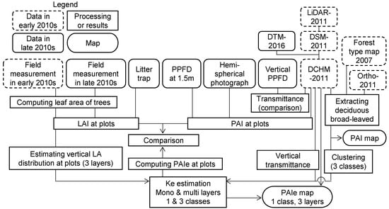
Figure 1.
Analysis flow.
2.1. Study Site
The study site was a deciduous secondary broad-leaved forest (centered at 137°25.5′E, 36°9′N, 3.4 × 2.5 km; a total of 3.1 km2 of broad-leaved forest) in the upper valley of the Namai River near Takayama, Gifu, central Japan (Figure 2). The topography is rather steep, with slopes between 30° and 40°, and elevation ranging between ca. 1080 m and 1490 m. The deciduous broad-leaved forest is surrounded by coniferous forest plantations composed of Japanese cedar (Cryptomeria japonica), Hinoki cypress (Chamaecyparis obtusa), and Japanese larch (Larix leptolepis). The deciduous secondary broad-leaved forest is composed of Mongolian oak (Quercus mongolica var. grosseserrata), Japanese umbrella tree (Magnolia obovata), and birch (Betula spp.), which occupy the upper tree layer. This secondary forest was used for harvesting firewood until the 1950s, as indicated by remnants of charcoal kilns, tree size after coppicing, testimony from a long-time resident, and visual interpretation of 1963 aerial photos obtained from the Forestry Agency of Japan. The secondary forests were mostly younger than 100 years old with simple canopy structure, and covered the whole study area.
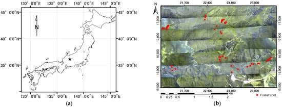
Figure 2.
Study site. (a) Location in Japan; (b) aerial photo of the study area in 2011. Red dots show locations of deciduous broad-leaved forest plots.
2.2. Forest Plot Survey
Plot surveys were undertaken between 2010 and 2012 for deciduous broad-leaved trees. Various height classes of stands were selected in the surveys, and circular plots were set in relatively homogeneous parts of stands. Plot radii varied between 5 and 17 m, based on tree height and tree density to control the number of sample trees in a plot. Plot radius was determined to be large enough to include at least 40 sample trees in each plot. Stem diameter (cm; 4 cm minimum usually) at a height of 1.2 m (DBH) of all trees was measured using calipers, and species names were recorded. Tree height (H, m) was measured using a Vertex hypsometer (Haglöf, Avesta, Dalarnas, Sweden) for all trees for which DBH was measured. Number of stems per plot was counted, and stem density was computed [51]. Geographic location of plots was determined with a GNSS receiver (either Mobile Mapper CX or Mobile Mapper 100, Thales, Arlington, VA, USA), and the coordinates were computed by the post-differential method. The survey records of 40 plots were used in this study (Figure 2). Data from all 40 plots were used for vertical LAI or LAD estimation. PPFD was measured for PAD estimation, hemispherical photographs were taken for PAI estimation, and litter traps were set for LAI measurement in 5 of the 40 plots with representative stand structure (Table 2) in 2019 and 2020. DBH and H were re-measured in 2019 or 2020 in each of the 5 plots to check changes after early 2010s. The stands were coppice forest because some trees sprouted bushes after logging at the base. Stands were arranged as plot 1, plot 5, plot 4, plot 3, and plot 2 in the order of the tree size from the smallest to the largest or the successional stage from the earlier to the latter. We estimated that the age of forest at plot 2 was less than 100 years.
Table 2.
Tree size data for the 5 plots in the 2010s.
2.3. Airbone LiDAR Data
Airborne LiDAR data (hereafter LiDAR data) were obtained during a helicopter flight on 28 August 2011 (LiDAR-2011); average pulse density was 4.83 points/m2 (DSM-2011, Table 3). A digital terrain model (DTM-2016) created using LiDAR data obtained by the Gifu prefectural government in October 2016 was also used to create a digital canopy height model (DCHM-2011) by subtracting DTM-2016 from DSM-2011. All of the remote sensing data were projected onto the Japanese plane rectangular coordinate system, zone 7 [75].
Table 3.
Summary of LiDAR observations.
2.4. Forest Type Map and Aerial Photography
A 2-m-mesh forest type map created using QuickBird imagery in 2007, LiDAR data from 2003 [76], and 0.5-m-mesh aerial ortho-photography (Figure 2) taken at the same time as the LiDAR measurements in 2011 were used for reference to identify broad-leaved forest.
2.5. Analysis
A total of 310 ha was selected for analysis in areas where the dominant vegetation was deciduous broad-leaved trees and there were no artificial structures, forest roads, open spaces, or rivers. Deciduous broad-leaved forests were selected using the forest type map [76] and aerial ortho-photography. Artificial structures, forest roads, open spaces, and rivers were excluded by using a terrain slope map computed with DTM-2016 and aerial ortho-photography. Areas in a 10 m buffer zone around excluded areas were also removed from the analysis. Average canopy height in the selected forests was 15.1 m on DCHM-2011.
2.5.1. Estimation of Leaf Area Using Allometric Equations
Allometric equations that compute leaf area per tree (LAT) were applied to all trees in the 40 plots, and vertical leaf distribution was computed using a Weibull distribution equation that approximated the distribution as described below. Leaf areas were summed by height in each plot, and LAI and vertical LAD distribution were estimated.
Allometric equations for computing LAT were created using data of 65 trees that were logged by Komiyama et al. [77] for an analysis of relative growth among tree parts of deciduous broad-leaved trees in Hida district, Gifu between 1990 and 1993. Trees were logged in Shoukawa village, Gifu and the Kuraiyama Experimental Forest of Gifu University [77] about 40 km west and 27 km southwest of our study site, respectively. The major species, Mongolian oak, painted maple (Acer mono), Japanese lime tree (Tilia japonica), Japanese red birch (Betula maximowicziana), and Kousa dogwood (Cornus controversa var. controversa), and ages of the trees in these areas were similar to those in our study site. Allometric equations for LAT estimation were created with Equation (3), which employs the least-squares method using the square of DBH (cm) multiplied by H (m).
where Y is LAT (m2 per tree), X is (DBH2 × H), and a and b are coefficients.
Y = aXb
The equations produced were applied to all trees in the 40 plots, and leaf area per plot (LAP) was estimated.
2.5.2. Estimation of Vertical Leaf Area Distribution
Vertical leaf area distribution was estimated by applying a Weibull distribution equation [33] to the computed LAT for all trees in the 40 plots. Cumulative leaf area CLA(Hn) (m2) from the tree top to height Z is expressed as follows [33]:
where Z is height from the ground (m), H is tree height (m), Hn is the normalized height of Z by tree height H, and β and ε are constants.
Leaf area density at layer j (LADj) in a plot is shown by Equation (5) as the vertical LAD distribution in 1 m height increments.
where N is number of vertical layers, CLAj (m2) is cumulative leaf area from the tree top to layer j, and Splot (m2) is area of the forest plot.
Utsugi [33] showed that the constants, β and ε, of the Weibull distribution equation are positively correlated with canopy length (CL) by tree height (CL/H) (p < 0.01) using felled stem samples of 26 trees (Japanese white birch, Betula platyphylla var. japonica; Mongolian oak; Castor aralia, Kalopanax pictus) logged in a 91-year-old deciduous broad-leaved forest near Sapporo, Hokkaido, Japan, as shown in Equations (6)–(8).
when CL/H < 0.55,
when CL/H > 0.55,
The relationship between H and CL (m) is as follows [33].
For Japanese white birch, it is
For other species, it is
The CL of all trees in the 40 plots in our study area was computed using Equations (9) and (10), and constants β and ε were computed for all trees using Equations (6)–(8). CLA(Hn) was computed using the LAT calculated with the allometric equations and Equation (4). Vertical LAD distribution in 1 m increments was computed for the 40 plots by applying Equation (5) to the computed CLA(Hn), and the vertical LAD distribution was then summarized for each plot.
2.5.3. LAI Measurement by Litter Trap
We conducted field measurements in 5 plots in 2019 and 2020; Plots 1–3 were measured in 2019 and Plots 4–5 in 2020. We set 2 litter traps in Plot-1, Plot-2, and Plot-3 in 2019 and in Plot-2, Plot-3, Plot-4, and Plot-5 in 2020. The traps were 1.0 m2 and placed 1.5 m above the ground. They were placed at least 10 m away from each other within each plot. Litter such as leaves, branches, and seeds were usually collected from the traps about once every 2 weeks from late August until mid-December. Litter was collected more frequently (once every 3 days) in October and November in 2020 to avoid disturbance by bear foraging.
Collected litter samples were dried in an oven at 60 °C for more than 48 h, then the litter was separated into leaves and other material (e.g., branches and seeds). Leaf dry weight in each trap was measured for each collection date. Approximately 10% of the dried leaves in each trap was reweighed, and their surface area was measured each time in 2019 and once every month in 2020 to compute the specific leaf area (SLA, m2 g−1). Leaves were fully spread and scanned (200 dpi) with an image scanner (GT-970, EPSON, Suwa, Nagano, Japan), and leaf area was computed from the scanned image. SLA was computed as the total leaf area divided by total weight of the sample. Total leaf area was computed by multiplying SLA by the total leaf weight in a litter trap on each collection day. The average SLA value before and after the sampling date was used to calculate total leaf area for samples without SLA sampling. Leaf areas were summed for each litter trap between the middle of August and the middle of December after defoliation and divided by the trap area to compute LAI (m2 m−2). The average LAI of the two traps was used as the LAI for each plot.
2.5.4. Effective PAI and Vertical Effective PAD Distribution Estimation
PPFD (mmol min−1 m−2) was measured on the forest floor (PPFD(I)) and in an open space (PPFD(I0)); rPPFD was then computed as PPFD(I) divided by PPFD(I0). Effective PAD (ePAD) and effective PAI (ePAI) were estimated using Equation (1), the Beer–Lambert law, and by setting the extinction coefficient K to 1 [25].
PPFD Measurement
Two photon sensors (SA-190, Li-Cor Lincoln, NB, USA) equipped with a data logger (CR800-4M or CR-1000, Campbell Scientific, Logan, UT, USA) were used to measure PPFD at Plot-1, Plot-2, and Plot-3 on 6 August 2019 and at Plot-2, Plot-3, Plot-4, and Plot-5 in early September 2020. Each photon sensor was attached to the top of 1.5-m-long steel pole that was placed upright, and the PPFD of the forest floor (I1.5m) was measured. In addition, the vertical PPFD distribution was measured at Plot-3 and Plot-5 between 1 and 10 September 2020. A 15 m surveying fiberglass grade rod was set to 10 m long and stood upright with four photon sensors attached at heights of 1.5 m (I1.5m), 4 m (I4m), 7.5 m (I7.5m), and 10 m (I10m) on the pole, and the vertical PPFD distribution was measured in each plot. Tree height around the 10 m pole was about 23 m in Plot-3 and 12 m in Plot-5.
We could not set any photon sensors above the canopies and did not measure downward solar PPFD (I0) in each plot. Therefore, downward solar PPFD was measured in 3 open spaces about 150–700 m from the plots as follows. Downward solar PPFD was measured at the top of a canopy observatory tower 25 m above the ground at the Takayama Flux Observatory for Plot-2 and Plot-3. Downward solar PPFD was measured with a photon sensor at the top of an upright 2 m steel pole in a large open space near Plot-1 and with an attached photon sensor (10 m high) on a surveying fiberglass grade rod in a small open space near Plot-4 and Plot-5. All PPFD measurements were made at 5 s intervals for 60 s; the 12 measurements were then averaged and recorded. PPFD in the period of stable records exceeding 100 mmol min−1 m−2 was selected to remove unreliable measurements, and the average rPPFD (I1.5m/I0,I4m/I0,I7.5m/I0,I10m/I0) of each photon sensor was computed for all plots.
Estimation of ePAI and Vertical Transmittance of PPFD
The Beer–Lambert law was applied to the PPFD data to estimate the ePAI and vertical ePAD distribution. PAD from height (h) above ground to the canopy top was computed with Equation (11), and when K = 1, it is the ePAD. The ePAD between the ground and the top of the canopy is ePAI. Since the photon sensors were set at 1.5 m above ground in all plots in our study, ePAI above 1.5 m was computed using Equation (11).
where PADh–top is the PAD from height h (m), which is 1.5 m, 4 m, 7.5 m, and 10 m above the ground, to the canopy top, Ih is the PPFD at h, I0 is the downward solar PPFD, and K is the extinction coefficient.
The transmittance of PPFD was computed at the sensor position (h = 1.5, 4, 7, and 10 m).
where TRh is transmittance of PPFD at h. The TRh was computed by applying Equation (12) to the measured PPFD in Plot-3 and Plot-5.
2.5.5. PAI Estimation Using Hemispherical Photographs
Hemispherical photographs were taken at 3 places in the 5 plots. A free software package (LIA32 ver. 0.3781 [78]) was used for the PAI calculation.
Taking Hemispherical Photos
Hemispherical photographs were taken at Plot-1, Plot-2, and Plot-3 on 9 September 2019 and at Plot-2, Plot-3, Plot-4, and Plot-5 on 28 August 2020. In 2019, a digital camera (Pentax Q10, Pentax, Tokyo, Japan) equipped with a standard zoom lens (SMC PN5-15BK, Pentax) and a fish-eye converter lens (Fit UWC-0195, Fit, Shimosuwa, Nagano, Japan) were set horizontally 1.5 m above the ground on a tripod to direct the lens perpendicular to the ground. Another digital camera (Canon 6D Mark II, Canon, Tokyo, Japan) equipped with a fisheye lens (Sigma 8 mm, Sigma, Kawasaki, Japan) was used in 2020 to take hemispherical photographs in the same way as in 2019. Photos were taken using the automatic exposure function by reducing exposure levels 3 to 6 times to avoid overexposure.
Computing PAI
PAI was computed using LIA32 [78] and the same algorithm that was used for LAI-2000 [79]. The parameters were set as follows: Pentax Q10 Projection: equidistance projection, field of view (FOV): 90.0°; Canon 6D Mark-II Projection: Sigma 8 mm (no aberration correction, built-in), FOV: 89.7°. The blue channel was used for PAI estimation. Prescribed values in LIA32 were used for other parameters such as binarization of photos.
2.5.6. Estimation of ePAI and Vertical ePAD Distributions Using LiDAR Data
DCHM-2011 was separated into cubes as described below, and ePAI and vertical ePAD distribution were computed using the Beer–Lambert law and the number of input and output pulses. We developed our own Fortran programs to preprocess the LiDAR pulse data. ArcGIS ver. 10.6 (ESRI, Redlands, CA, USA) was used for image processing, and JMP 11 (SAS, Cary, NC, USA) was used for statistical analyses.
Pre-Processing
Almedia et al. [25] have pointed out that pulse density influences the accuracy of LAI estimation. They have recommended a 10 m mesh for the stable analysis of ePAI and vertical ePAD distribution for pulses with a density of 1 to 15 points m−2. The pulse density of DCHM 2011 varied greatly due to the pitching of the platform (i.e., the helicopter) by keeping a consistent flight altitude above the ground. The maximum point density of DCHM-2011 was controlled up to 10 points m−2 by random sampling to reduce variation in the accuracy of LAI estimates caused by differences in pulse density. The average point density was 5.75 m−2 over the target deciduous broad-leaved forests after resampling. The resampled DCHM-2011 text data were divided into 1 m cubes, and the number of pulses in each cube was counted. The number of pulses was stored for each cube position in a multi-layer raster file (hereafter, the Cube-raster file).
Summarizing the Number of Pulses in Cubes
The Cube-raster file was summarized to adjust the position to be compatible with the vertical LAD estimation of the other methods for comparison as follows.
LA: multi-layer data of DCHM points; used to compare with results of allometric equations.
LA height layers: height 1.2 m below ground ≤ Height (H) < 1.0 m above ground (ground surface, LA0), 1.0 ≤ H < 2.0 m (herb layer, LA1), 2.0 ≤ H < 3.0 m (LA2), 3.0 ≤ H < 4.0 m (LA3), 4.0 ≤ H < 5.0 m (LA4) …… 29.0 ≤ H < 30.0 m (LA29) above ground.
LP: multi-layer data of DCHM points; used to compare with estimates by rPPFD.
LP height layers: 1.2 m below ground ≤ DCHM < 1.0 m above ground (ground surface, LP0), 1.0 ≤ DCHM < 1.5 m (herb layer, LP1), 1.5 ≤ DCHM < 4.0 m (LP2), 4.0 ≤ DCHM < 7.0 m (LP3), 7.0 ≤ DCHM < 10.0 m (LP4), and 10.0 ≤ DCHM < 30.0 m (LP5).
A cylinder with a radius of 10 m was set at the center coordinate of each plot, and DCHM points for cases LA and LP were extracted. The number of total pulses (−1.2 m ≤ DCHM < 30.0 m) and number of pulses less than or equal to the herb layer (number of understory layer pulses, H < 2.0 m) were then summarized. The 1-m-mesh Cube-raster file was summarized as 10-m-mesh data, and the calculated number of total pulses and understory layer pulses were summarized in each mesh to estimate PAI. Since we analyzed LAI of trees and there were few tree leaves below 2 m, difference of the herb layer height between LA and LP was neglected.
ePAD Estimation Using the Beer–Lambert Law
The vertical ePAD distribution was estimated by using the summarized DCHM-layer pulse data as follows. Numbers of pulses entering a layer from above and penetrating through the layer were counted. Pulses that were not reflected in a given layer were assumed to enter the layer below.
where Pj is the number of pulses reflected at layer j, n is the number of layers, Iini is the number of pulses entering from above, and Iouti is the number of pulses passing through layer i.
The Beer–Lambert law was applied to calculate the vertical ePAD distribution using Equation (15).
where PADi is the PAD in layer i, and K is the extinction coefficient. If K = 1, it is the ePAD.
PAI is the sum of the PAD of all layers:
where the PADs of layer 2 (LA2 or LP2) and higher were summed, and the herb layer was excluded in the analysis.
Equations (13)–(16) were applied to cylindrical DCHM pulses LA and LP, which were extracted at the 40 plots, and the vertical ePAD distributions were estimated with K = 1. The Beer–Lambert law with K = 1 was also applied for the 10-m-mesh DCHM LA of the LiDAR data as well and summed to create an ePAI map. Transmittance at the same height as the vertical PPFD measurement was also computed:
where I0 is number of pulses over the plot, Iinh is number of pulses reaching height h (m), and TRLh is the transmittance of pulses at h.
Estimation of PAI and Vertical PAD Distribution Using LiDAR Data with an Empirically Estimated Ke
Extinction coefficients in the 40 plots were estimated by dividing the vertical ePAD distribution by the vertical LAD distribution estimated using tree measurement data. Before estimating Ke, the vertical ePAD distribution of DCHM-2011 and the vertical LAD distribution of field plot data were standardized at 1 to be the maximum canopy height within each plot. Forest canopy was classified into 3 layers as 0–33, 34–66, and 67–100 (%) from the ground to the maximum canopy height, and ePAD and LAD were summarized in each layer and all layers 0–100 (%). Values of Ke were computed using the summarized ePAD and LAD and Equations (18)–(21) in the 40 plots.
where (0–33), (34–66), and (67–100) indicate each of the three respective height layers and (0–100) shows the whole canopy.
Meshes with similar vertical ePAD distributions in the vertical ePAD distribution map were segmented as a polygon file using the segmentation function in ArcGIS. The segments were classified into 3 forest types using the vertical ePAD distribution data and Ward clustering [80] of JMP 11 to evaluate the effects of forest structure on a PAI map [64].
The estimated Ke values were summarized, and Ke values to be applied to each forest type were determined. The PAI and vertical PAD distribution were estimated using DCHM-2011 and the appropriate Ke. A PAI distribution map was produced using DCHM-2011 and the Beer–Lambert law with the most favorable Ke.
3. Results
3.1. Vertical Leaf Area Distribution by Allometric and the Weibull Distribution Equation
We performed a regression analysis to produce allometric equations for LAT estimation using the logged sample trees by Komiyama et al. [77]. The square of DBH multiplied by H (DBH2H) was used as an independent variable in a least-squares regression analysis. The relationship between LAT and DBH2H was different for birch species and other species. Similar to the relationships between canopy length and tree height (Equations (9) and (10)), birch spp. seemed to have a unique canopy structure. We therefore derived Equation (22) using 12 Japanese white birch and Japanese red birch and Equation (23) using 52 Mongolian oak, Kousa dogwood, Japanese umbrella tree, maple spp., and Japanese bird cherry (Prunus grayana). The coefficient of determination (r2) for Equation (22) for birch was lower than that for Equation (23), and the estimation bias of leaf area may be large. Komiyama et al. [77] have pointed out that using branch height as an explanatory variable improved the accuracy of their leaf dry weight estimation model. However, we did not measure branch height because the primary objective of the plot surveys in the early 2010s was estimating stem volume using DBH and H [51]. It might reduce the accuracy of leaf area estimation.
where LAT is leaf area of a tree (m2) and D2H is DBH2H (cm2 m).
Using these equations, we estimated the vertical LAD distribution for each tree and summarized it for each plot in 1 m layers up from the ground using the LAT and the Weibull distribution Equation (5) [33]. The distribution was unique in each plot (Figure 3a). LAD was the greatest at about 4 to 6 m below the tree tops. This trend became clearer when the tree height varied among trees in the upper canopy layer. Large Mongolian oak trees dominated in Plot-2, while birch spp. and many other species grew in other plots, and successional stages (from early to late) were in the order of Plot-1, Plot-5, Plot-4, and Plot-3 (Table 2).
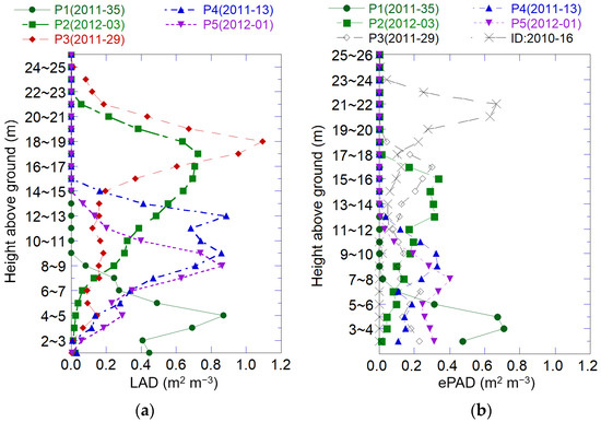
Figure 3.
Vertical distribution of LAD and ePAD in 1 m intervals for 5 plots (P1~5). (a) LAD estimated using plot survey data, allometric equations, and the Weibull distribution equation. (b) ePAD estimated using DCHM-2011 and the Beer–Lambert law with K = 1. Pulses did not pass through the upper canopy in plot ID 2020-16.
3.2. LAI Estimation Using Collected Litter
LAI was computed using the SLA and collected litter samples (Table 4). The LAI in plots differed in 2019 and 2020. LAI was in the order of Plot-3 > Plot-2 > Plot-1 in 2019, but Plot-2 > Plot-4 > Plot-3 > Plot-5 in 2020. Moreover, LAI was greater in Plot-2 and Plot-3 in 2020 than in 2019. Annual variation was great in Plot-2, where the value was 1.35 times higher in 2020 than in 2019. The trap cloth in one trap in Plot-1 was partially floating in 2019, and the amount of litter in that trap was only 7% of that in the other. Litter was probably lost due to the wind, and LAI was therefore most likely underestimated.
Table 4.
Estimated LAI and PAI by litter, PPFD, and hemispherical photography.
3.3. ePAI Estimation by PPFD and PPFD Vertical Transmittance
PPFD at 1.5 m was measured on 6 August 2019 in Plot-1, 2 and 3. PPFD at 1.5 m was measured in Plot-2 and Plot-4, and vertical PPFD was measured in Plot-3 and Plot-5 on 1, 9, and 10 September 2020. The respective dates and plots of the PPFD measurements are given in Table 4. ePAI was computed using these measurements and the Beer–Lambert law with K = 1. In 2019, the maximum ePAI value (3.22) was found in Plot-3, and the minimum (2.20) was in Plot-2. In 2020, the maximum ePAI (2.97) was in Plot-3, and the minimum (2.41) was in Plot-4. The ePAI was greater in Plot-3 than in Plot-2 in 2019 and 2020 (Table 4). Vertical PPFD transmittance differed between Plot-3 and Plot-5 (Figure 4a). The forest in Plot-3 was mature with top-layer trees (20% of trees) averaging about 22.7 m in height, whereas the forest in Plot-5 was younger, with top-layer trees about 13.0 m tall in 2020. Much of leaves existed at heights greater than 10 m to the canopy top in Plot-3 and varied from the bottom to near the canopy top in Plot-5 (Figure 4).
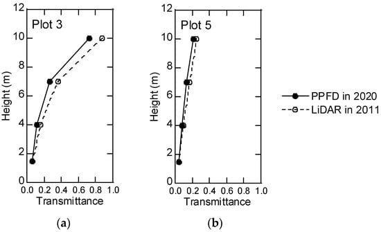
Figure 4.
Vertical transmittance in PPFD measurements and LiDAR pulses: (a) Plot-3, (b) Plot-5.
3.4. PAI Estimated by Hemispherical Photography
The respective dates and plots of the hemispherical photos are given in Table 4, along with the PAI values. Photos were taken at dawn, in the evening, or during overcast conditions with scattered light. However, a few photos had uneven brightness.
3.5. ePAI and Vertical ePAD Distribution Estimated by LiDAR Data
LiDAR pulses reached the ground in most plots as shown in Figure 3b, and the canopy structure was observable. Although dense leaves reflect pulses at the upper canopy, blocking pulses from reaching the ground, an average of 0.69 points m−2 was observed on the ground. The vertical ePAD distribution clearly shows the underlayer structure in Figure 3b. However, small trees and branches in the underlayer were not observed (Plot ID 2010-16) among the 40 plots, because pulses did not reach the underlayer (Figure 3b). The number of incident pulses was 2.49 points m−2, but the number of pulses in the plot was 0.19 points m−2 at 10 m above the ground, and was very low compared to the other plots. It suggests that ePAI may not be estimated in forest with very dense canopy leaves by DCHM-2011. Plot 2010-16 was excluded from the following analysis.
Vertical pulse transmittance was computed in Plot-3 and Plot-5 (Figure 4). The decrease in pulse transmittance from the top to the bottom of the stand was very similar to that computed by PPFD in Plot-5, but the LiDAR value was greater than the PPFD value at 10 m in Plot-3. The distribution of ePAI was rather homogeneous in a large part of the forest (Figure 5). The maximum, minimum, average, and standard deviation of the estimated ePAI values were 6.86, 0.0, 3.0, and 0.88, respectively, in the ePAI map in the study area.
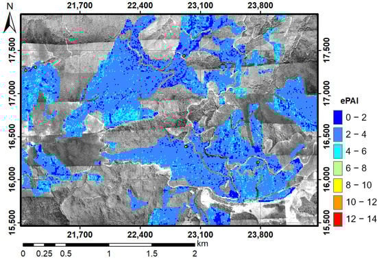
Figure 5.
Map of the ePAI distribution using DCHM-2011 and the Beer–Lambert law with K = 1. The background is the red channel of aerial ortho-photography in 2011.
3.6. PAI Estimation Using LiDAR Data and Empirically Estimated Ke
3.6.1. Estimating Ke
Histograms and box-and-whisker plots of empirically estimated Ke values for 3 normalized vertical layers (0–33, 34–66, 67–100%) and all layers (0–100%) are shown in Figure 6. The median Ke was smaller in higher canopies with more leaves than in the lower parts. Some plots had notable outliers. Because the ePAD estimated by DCHM-2011 including all data would have been too small and the LAD estimated using field plot data would have been too large. The plots with outlier Ke values were excluded from the computed statistics shown in Table 5.
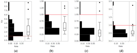
Figure 6.
Histograms and box-and-whisker plots of empirically estimated Ke at a height of (a) 0–33 (%), (b) 34–66 (%), (c) 67–100 (%), and (d) 0–100 (%). The horizontal lines in the middle of each right box shows the median, and the bottom and top edges of box show the 25th and 75th percentiles, respectively. Whiskers show 1.5 times a quartile; pulses out of the whisker range were considered to be outliers. The red line shows K = 1 which is used for ePAI estimation.
Table 5.
Ke statistics in the 3 vertical layers computed using DCHM-2011.
3.6.2. Forest Type Classification Map
The forest type map showed three forest types, as classified by the Ward method (Figure 7). Plot-2 and Plot-3 were classified as forest type 1, in which tree bodies converged at heights over 10 m. Plot-4 and Plot-5 were forest type 2, in which tree bodies converged between heights of 5 m and 10 m. Plot-1 was classified as forest type 3, in which tree bodies converged between heights of 2 m and 5 m.
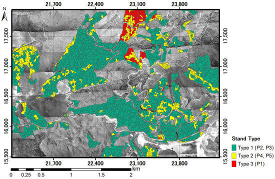
Figure 7.
Forest type map by segmentation of DCHM-2011 using the Ward method. Plot-2 and Plot-3 belong to type 1, Plot-4 and Plot-5 belong to type 2, and Plot-1 to type 3. The canopy height was in the order (tallest to shortest): Type 1 > Type 2 > Type 3.
3.6.3. Estimating Ke, PAI, and Vertical PAD Distribution
Ke was estimated for each forest type shown in Figure 7. The outlier plots in Figure 6 were excluded from the estimation, and Ke was summarized for each forest type (Table 6). The vertical PAD distribution and PAI were computed using DCHM-2011, the Beer–Lambert law, and the derived Ke in each segment.
Table 6.
Ke statistics in the 3 vertical layers of the 3 forest types.
3.7. Comparison of Estimated LAI, Vertical LAD Estimation, PAI, and Vertical PAD Distribution
In this section, we compare the LAI, LAD, PAI, and PAD values generated from the field measurements and estimation methods.
3.7.1. Comparison of Estimates Using Litter Traps and Plot Survey Data
There was a linear relationship between LAI estimated by the plot data and the allometric equations and LAI measured by litter traps in 2019 and 2020 in the 5 plots (Figure 8, p < 0.001). LAI values estimated using the allometric equations were about 1.3 times of those computed by litter trap measurements.

Figure 8.
Relationship between LAI estimated by allometric equations and litter trap measurements.
3.7.2. Comparison of Estimates Using LiDAR and Forest Plot Data
The vertical PAD distribution and PAI were computed using the ePAD derived from DCHM-2011 and the average Ke values in Table 5 and Table 6. The PAI estimated for the 3 canopy layers from the ground to the top (0–33, 34–66, and 67–100%) using the Ke for each layer (Table 5 and Table 6) is labelled PAI (Ke: multi), and the PAI estimated using the Ke for the whole layer (0–100%) is called PAI (Ke: mono). The PAIs estimated using the Ke for the 3 forest types and the Ke for all plots were named PAI (Ke: type) and PAI (Ke: all), respectively. Four PAIs were estimated with these combinations of layer and forest type selections. The relationship between LAI estimated by the allometric equations and the 4 PAIs was examined with a regression analysis and scatter diagrams (Figure 9).
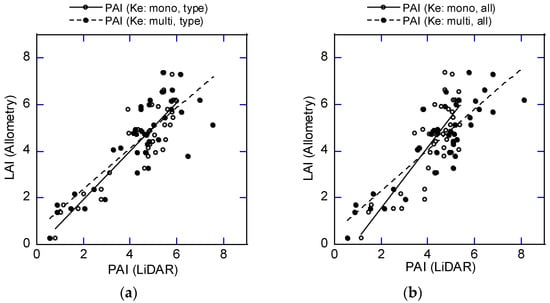
Figure 9.
Relationship between LAI estimated by allometric equations and PAI estimated using DCHM-2011. (a) The case of LAI and PAI estimated for 3 forest types separately. (b) The case of LAI and PAI estimated as 1 forest type. Mono represents the case where LAI and PAI were estimated as 1 layer. Multi is the case where LAD and PAD were estimated in the three layers and summed. “Type” and “all” refer to the individual forest types and the combined forest, respectively.
Ke: mono, type
Ke: multi, type
Ke: mono, all
Ke: multi, all
where LAI is the LAI estimated by the allometric equations, and PAI is the PAI estimated using DCHM-2011 and the Beer–Lambert law with the respective estimated average Ke values shown in Table 5 and Table 6.
The relationships in Equations (24)–(27) were all significant (p < 0.001). The case of Ke (mono, type) had the closest offset to the origin, closest slope to 1, and the greatest coefficient of determination, but the estimates seemed to be saturated at a PAI of 6 (Figure 9a). On the other hand, the estimates did not become saturated with Ke (multi, all), which had the second highest coefficient of determination (Figure 9b). This supports applying Ke (multi, all) to produce a PAI distribution map using DCHM-2011. Estimating PAI using Ke (multi, type) may be risky because there were only seven plots for forest type 2 and type 3 in the Ke estimation, and the number of pulses in each layer may be insufficient to obtain an accurate estimate. A PAI distribution map was produced using DCHM-2011 and the Beer–Lambert law with Ke (multi, all) (Figure 10). Forest type 3, which has the lowest canopy height (Figure 7), had the lowest PAI. On the other hand, forest type 1 (the tallest) had the largest area and a wide range of PAI. However, areas with high PAI values (>10) were located areas with steep slopes (>30°) and cliffs. Steep slope angles and sharp changes would introduce estimation errors.
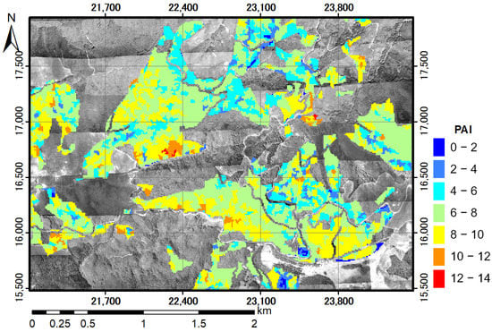
Figure 10.
Map of PAI distribution estimated using DCHM-2011 and the Beer–Lambert law with different Ke values for the three layers and all plots (Ke: multi, all). The applied values of Ke were 2.15, 0.52, and 0.30 for the 0–33, 34–66, and 67–100% height layers, respectively (Table 5). The background is the red channel of aerial ortho-photography in 2011.
3.7.3. Comparison of Transmittance between LiDAR Pulse and PPFD
Estimated transmittance of pulses in DCHM-2011 and PPFD measurement showed a similar attenuation pattern relative to the height above ground (Figure 4). The average tree height of the top 20 trees (about 25% of all trees in Plot-3) was 20.4 m in 2011 and 22.7 m in 2019. The top photon sensor (10 m) was situated under the leaf canopy. Therefore, PPFD was attenuated at the canopy leaf layer and reached the top sensor. As the result, transmittance of PPFD at 10 m was smaller than DCHM-2011. On the other hand, transmittance changes were very similar to each other in Plot-5. The average height of the top 20 trees was 11.1 m in 2012 and 13.4 m in 2020. Thus, the top photon sensor (10 m) almost reached the top of the leaf layer in Plot-5.
3.7.4. Comparison of All LiDAR and Field Estimations
The LAI measurements can be classified into two patterns in the field estimations (Figure 11). The first pattern is that the estimated LAI was greater in Plot-2, Plot-3, and Plot-4 than that in Plot-1 and Plot-5 for the estimation by allometric equations and litter traps. The second is that the estimated PAI was greater in Plot-3 and Plot-5 than that in Plot-2 and Plot-4 for the estimation using hemispherical photography and ePAI by rPPFD (K = 1). On the other hand, the PAI estimated using DCHM-2011 varied among the plots when different Ke values were used (Figure 11). PAI (Ke: multi) showed a similar relation among plots as PAI estimated by allometric equations, while PAI (Ke: mono) showed a similar relationship among plots to PAI estimated by hemispherical photography. These trends were the same between PAI (Ke: type) and PAI (Ke: all) even when the forest types were classified. The ePAI estimated using DCHM-2011 with K = 1 was similar to the estimation by rPPFD with K = 1.
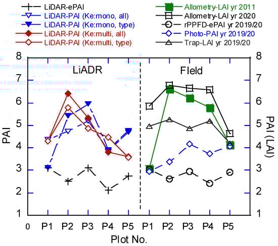
Figure 11.
Comparison of LAI and PAI estimates using LiDAR data (DCHM-2011) and field measurements by different methods. Ke multi, all, and type are defined in Figure 9.
Estimates of PAD using DCHM-2011 and LAD using the allometric equations were compared in Plot-3, forest type 1 (Figure 12). Vertical PAD distributions differed among LiDAR estimations with different Ke assignments. The LiDAR ePAD using K = 1 was clearly smaller than the allometry-derived LAD, but ePAD became slightly greater at height below 8 m than that over 8 m. The LiDAR PAD (Ke: mono) showed a similar vertical PAD distribution pattern to that of LiDAR ePAD, but the magnitude was almost twice as large. The LiDAR PAD (Ke: multi) had the clearest and greatest PAD peak (at 16 m) among the LiDAR estimates. The vertical distribution was similar to that of the allometry-derived LAD with smaller LAD at the lower part than that at the upper canopy. The LiDAR PAD (Ke: multi) had vertical PAD distribution most similar to the allometry-derived LAD.

Figure 12.
Estimates of PAD or LAD using DCHM-2011 and the allometric equations in Plot-3.
4. Discussion
4.1. Appropriateness of Field Measurements
There are some measurement records of LAI and PAI in a type 1 forest (i.e., Plot-2 and Plot-3 in this study) near the center of our study area [41,74,81]. Therefore, we compared those measurement records with our own to check the reliability of our field measurements. Although those studies measured seasonal changes of LAI or PAI, we compared the annual maximum values of their measurements with ours.
The LAIs were determined to be 3.9–5.3 (m2 m−2) in Plot-2 and Plot-3 by litter trap measurements in 2019 and 2020 (Table 4). This was close to the maximum LAI value (5.3 m2 m−2) found by litter trap measurement that incorporated vertical changes of leaf mass per area in 2006 and 2007 by Nasahara et al. [41]. This is the only published case of litter trap measurement that accounted for vertical canopy structure, and the estimate is most likely close to the true LAI. At the same time of the litter trap study, a PAI measurement using LAI-2000 resulted in a PAI of 3.3 (m2 m−2), about 60% of the litter trap estimate [41]. Another PAI estimate using hemispherical photography was 4.0 [81]. Our PAI estimates by hemispherical photography using the LAI-2000 algorithm were 2.9 and 3.1 in 2019 and 3.4 and 4.2 in 2020, close to the value of Muraoka and Koizumi [81]. Muraoka et al. [74] estimated that PAI was 6.5 ± 0.4 using PPFD measurements with K = 0.46 in 2003 and 2007. When we applied the same K to our PPFD measurements in 2019 and 2020, PAI was 5.7–6.5.
Therefore, the LAI or PAI values estimated from our measurements by litter trap, hemispherical photography, and PPFD were similar to those estimated by the same methods in a type 1 forest in other studies. However, each method resulted in different estimates. PAI and LAI values estimated by hemispherical photography or LAI-2000 were about a half those of litter trap measurements, which are assumed to be the most accurate (Table 4, Figure 11).
LAI estimated by the allometric equations was similar to LAI estimated by litter traps in Plot-1 and Plot-5, which had small, young trees (Table 2). On the other hand, LAI estimated by the allometric equations was greater in Plot-2, Plot-3, and Plot-4, which had tall trees. There must be a few causes of this trend. First of all, the maximum size of sample trees that were used to produce the allometric equations were as follows: 31.7 cm and 38.1 cm for DBH and 25.6 cm and 24.9 m for H for birches and other trees, respectively [77]. Oak trees were dominant in Plot-2, with a maximum DBH and H of 45.5 cm and 21.5 m, respectively. Birches were dominant in Plot-3, with a maximum DBH and H of 36.0 cm and 24.3 m, respectively. Thus, the DBH of some trees in these two plots exceeded the maximum of the sample trees used to produce the allometric equations. The coefficient of determination of 0.644 for the birch equation suggests that the allometric relationship between DBH, H, and leaf amount varies. Therefore, the LAT estimation accuracy might be not high.
The second possible cause is natural pruning. The canopy length (i.e., leaf amount) varies by location in forests due to different light conditions even if DBHs are the same [77]. Komiyama et al. [77] used lower branch height for leaf dry weight estimation. We did not measure lower branch height and instead used DBH2H for leaf area estimation, which may have been greater than that of the litter trap measurement.
4.2. Validation of Empirically Estimated Extinction Coefficient Ke
Extinction coefficients (Ke) were estimated as ratios of vertical ePAD distributions (estimated using DCHM-2011) and vertical LAD distributions (estimated using tree measurements in 40 plots). As noted in the previous section, the allometric equations yielded relatively high estimates of leaf area in old forests. Therefore, the estimates of Ke may be relatively low. Various factors influence K estimation using LiDAR data, such as distribution of leaf inclination angle, leaf clumping, beam size, pulse intensity, incidence angle of pulse, and laser wavelength [25].
Of the factors listed above, the relationship between the distribution of leaf inclination angle (θleaf) and incidence angle of pulse (θlidar) is the most important because K is defined as cos(θleaf)/cos(θlidar) (Equation (2)) [71]. When the pulse incidence angle is small enough (θlidar ≤ ±10°), the effects of cos(θlidar) are small, and K is equal to cos(θleaf) [11,72]. When leaf inclination angle (α) is constant, K is a function of α, i.e., K = cos(α) where α + θ ≤ 90° where θ is beam incident angle [69]. LiDAR-2011 was scanned with a scan angle of ±30°, and leaf angle was calculated using Equation (2). The calculated leaf angles, using the average Ke values in Table 5 with a scan angle of ±30°, are as follows: about 0° in layer 0–33%, 59°–63° in layer 34–66%, 72°–75° in layer 67–100%, and 59°–63° for the whole canopy (0–100%). Thus, the leaf angle changed from upright to almost horizontal from the top to the bottom of the canopy. The Ke in the lowest layer (0–33%) was 2.15 because there were few leaves there, and pulses hit branches and stems. The estimated Ke in the other layers agreed well with reported leaf inclination angles and K values. The Ke of 0.52 for the whole canopy was very close to 0.5, which is the value derived assuming spherical leaf angle distribution and is used for various types of forests [11].
4.3. Importance of Applying Vertically Distinct Ke
Applying vertically distinct values of Ke in forest layers yielded much more accurate PAD distributions than did treating the forest as a single layer with an average Ke (Figure 12). Estimates of PAI and vertical PAD distribution using DCHM-2011 with vertically distinct values of Ke were similar to the estimates of LAI and vertical LAD determined by using allometric equations (Figure 9, Figure 11 and Figure 12). Methods that treat the canopy as a single layer such as LiDAR-PAI (Ke: mono), hemispherical photography, and relative PPFD measurement with one quantum sensor on the ground underestimated PAI (Figure 11). The use of vertically distinct Ke values improved the accuracy of LAD estimation, particularly in the upper canopy (Figure 12), which has dense leaves with large inclination leaf angle. Figure 10 shows the usefulness of vertically distinct Ke values. Fine PAI distribution patterns and difference of PAI among 3 forest types are clearer than that in Figure 5 in which ePAI is shown treating the canopy as single layer.
Vertical canopy structure affects the physical environment under canopies [33]. Therefore, mapping the vertical PAD structure in large forests is important to better understand the function of canopies, and it should be a topic of future research. It is important to estimate Ke using airborne LiDAR data and known vertical LAD or PAD distributions or to set Ke for distinct vertical layers by measuring leaf angle distribution accurately to estimate PAI and vertical PAD using the Beer–Lambert law.
5. Conclusions
We examined the performance of LiDAR data in deciduous broad-leaved forest in Takayama, Gifu, Japan, for estimating vertical and horizontal leaf area distributions. We estimated ePAI and vertical ePAD distribution by applying the Beer–Lambert law with K = 1 to DCHM-2011. We also estimated LAI and vertical LAD distribution of trees or plots using allometric equations and a Weibull distribution equation. We then estimated extinction coefficients for three height layers from the ground to the canopy top using the estimated ePAI and vertical ePAD distribution. The estimated values of Ke were almost the same as those computed using traditional leaf angle distribution.
It is important not to allocate a single Ke to the entire canopy as single layer, but rather to allocate vertically distinct Ke values to multiple height layers for accurate estimation of PAI and vertical PAD distribution using the Beer–Lambert law. The derived LAI had a linear relationship with LAI determined by litter trap measurements, a relationship that was not observed with estimates that treated canopies as single layer, for example, hemispherical photography or relative PPFD. The Beer–Lambert law, with independent Ke in vertical layers, must be incorporated in order to make an accurate PAI or LAI estimation.
The use of LAI and a vertical LAD distribution, which are estimated by applying allometric equations to tree measurements to estimate leaf area per tree and applying the Weibull distribution equation to the leaf area, is effective for estimating Ke in vertical layers using airborne LiDAR data. Determining the causes of outliers of Ke and large variation of Ke near the ground in the lowest forest layer, removing the causes in the Ke estimation, and obtaining more measurement data are still needed to improve this method of estimating 3D leaf area distribution using airborne LiDAR data.
The young secondary forests have quite simple canopy structures compared to that of old growth. The simple structures would result in excellent PAI estimation. Therefore, validation of this method is a future research topic in old growth stands of deciduous broad-leaved forests with initially complex canopy structures. Thus, the applicability of the method should be examined in other forest ecosystems. Topographic effects on steep slopes should also be studied for accurate PAI mapping and for clarifying any limitations of this method.
Author Contributions
Conceptualization and methodology, Y.A.; resources and software, Y.A.; formal analysis, K.A.; field survey, Y.A. and K.A.; data curation, K.A.; visualization, K.A. and Y.A.; writing—original draft preparation, K.A.; writing—review and editing, Y.A.; supervision, Y.A.; research administration and funding acquisition, Y.A. All authors have read and agreed to the published version of the manuscript.
Funding
This study was supported by JSPS KAKENHI (grant number 19K06123, “Development of methodology for 3D canopy structure analysis of deciduous broadleaved forest”, Grant-in-Aid for Scientific Research C). This research was also executed in the master course program by Gifu University’s fund.
Data Availability Statement
The data presented in this study are available on request from the corresponding author after concluding a joint research agreement with the River Basin Research Center of Gifu University. Restrictions apply to the availability of LiDAR 2016 (DTM). These data were obtained from the Gifu Prefecture Government and are available by applying for use of them from the prefecture.
Acknowledgments
We express heartfelt gratitude to Yasuyuki Maruya, a former research associate of the River Basin Research Center (currently an assistant professor at Kyushu University), and Kouji Suzuki and Hajime Hiratsuka, staff members of Takayama Research Center, River Basin Research Center for their support in the field survey. We also express our gratitude to Fuku Uekanekuri and Yuka Nishio (Faculty of Applied Biological Sciences at that time) at Gifu University. The 2016 LiDAR data were provided by the Gifu Prefecture Government. We also express our gratitude to the government and its staff who supported our study. We give special thanks to the editors and the three anonymous reviewers for their valuable comments and suggestions on our manuscript.
Conflicts of Interest
The authors declare no conflict of interest.
References
- Jones, H.G. Plants and Microclimate: A Quantitative Approach to Environmental Plant Physiology, 3rd ed.; Cambridge University Press: Cambrige, UK, 2014; p. 407. [Google Scholar]
- Chapin, F.S., III; Matson, P.A.; Mooney, H.A. Principles of Terrestrial Ecosystem Ecology; Sringer-Verlag: New York, NY, USA, 2002; p. 436. [Google Scholar]
- Kato, A.; Tamura, T.; Ichihashi, A.; Kobayashi, T.; Takahashi, T. An automatic method to estimate forest coverage and strata from terrestrial laser data. J. Jpn. Soc. Reveget. Tech. 2019, 45, 121–126, (In Japanese with English Summary). [Google Scholar]
- Murai, H.; Higuchi, H. Factors affecting bird Species diversity in Japanese forests. Strix 1998, 7, 83–100, (In Japanese with an English Summary). [Google Scholar]
- Clawges, R.; Vierling, K.; Vierling, L.; Rowell, E. The use of airborne lidar to assess avian species diversity, density, and occurrence in a pine/aspen forest. Remote Sens Environ. 2008, 112–115, 2064–2073. [Google Scholar] [CrossRef]
- Melin, M.; Matala, J.; Mehtätalo, L.; Pusenius, J.; Packalen, P. Ecological dimensions of airborne laser scanning—Analyzing the role of forest structure in moose habitat use within a year. Remote Sens. Environ. 2016, 173, 238–247. [Google Scholar] [CrossRef]
- Martinuzzi, S.; Vierling, L.A.; Gould, W.A.; Falkowski, M.J.; Evans, J.S.; Hudak, A.T.; Vierling, K.T. Mapping snags and understory shrubs for a LiDAR-based assessment of wildlife habitat suitability. Remote Sens. Environ. 2009, 113, 2533–2546. [Google Scholar] [CrossRef]
- Monsi, M.; Saeki, T.; Schortemeyer, M. On the factor light in plant communities and its importance for matter production. Ann. Bot. 2005, 95, 549–567. [Google Scholar] [CrossRef]
- Asner, G.P.; Scurlock, J.M.O.; Hicke, J.A. Global synthesis of leaf area index observations: Implications for ecological and remote sensing studies. Glob. Ecol. Biogeogr. 2003, 12–13, 191–205. [Google Scholar] [CrossRef]
- Goodwin, N.R.; Coops, N.C.; Culvenor, D.S. Assessment of forest structure with airborne LiDAR and the effects of platform altitude. Remote Sens. Environ. 2006, 113, 2317–2327. [Google Scholar] [CrossRef]
- Richardson, J.J.; Moskal, L.M.; Kim, S.H. Modeling approaches to estimate effective leaf area index from aerial discrete-return LIDAR. Agric. For. Meteorol. 2009, 149, 1152–1160. [Google Scholar] [CrossRef]
- Falkowski, M.J.; Evans, J.S.; Martinuzzi, S.; Gessler, P.E.; Hudak, A.T. Characterizing forest succession with lidar data: An evaluation for the Inland Northwest, USA. Remote Sens. Environ. 2009, 113–115, 946–956. [Google Scholar] [CrossRef]
- Zhao, K.; Popescu, S. Lidar-based mapping of leaf area index and its use for validating GLOBCARBON satellite LAI product in a temperate forest of the southern USA. Remote Sens. Environ. 2009, 113, 1628–1645. [Google Scholar] [CrossRef]
- Leeuwen, M.; Nieuwenhuis, M. Retrieval of forest structural parameters using LiDAR remote sensing. Eur. J. Forest Res. 2010, 129, 749–770. [Google Scholar] [CrossRef]
- Korhonen, L.; Korpela, I.; Heiskanen, J.; Maltamo, M. Airborne discrete-return LIDAR data in the estimation of vertical canopy cover, angular canopy closure and leaf area index. Remote Sens. Environ. 2011, 115, 1065–1080. [Google Scholar] [CrossRef]
- Peduzzi, A.; Wynne, R.H.; Fox, T.R.; Nelson, R.F.; Thomas, V.A. Estimating leaf area index in intensively managed pine plantations using airborne laser scanner data. For. Ecol. Manag. 2012, 270, 54–65. [Google Scholar] [CrossRef]
- Stark, S.C.; Leitold, V.; Wu, J.L.; Hunter, M.O.; de Castilho, C.V.; Costa, F.R.C.; Mcmahon, S.M.; Parker, G.G.; Shimabukuro, M.T.; Lefsky, M.A.; et al. Amazon forest carbon dynamics predicted by profiles of canopy leaf area and light environment. Ecol. Lett. 2012, 15, 1406–1414. [Google Scholar] [CrossRef]
- Hopkinson, C.; Lovell, J.; Chasmer, L.; Jupp, D.; Kljun, N.; van Gorsel, E. Integrating terrestrial and airborne lidar to calibrate a 3D canopy model of effective leaf area index. Remote Sens. Environ. 2013, 136, 301–314. [Google Scholar] [CrossRef]
- Sabol, J.; PatoČka, Z.; Mikita, T. Usage of LiDAR data for leaf area index estimation. GeoScience Eng. 2014, 60–63, 10–18. [Google Scholar] [CrossRef]
- Palace, M.W.; Sullivan, F.B.; Ducey, M.J.; Treuhaft, R.N.; Herrick, C.; Shimbo, J.Z.; Mota-E-Silva, J. Estimating forest structure in a tropical forest using field measurements, a synthetic model and discrete return lidar data. Remote Sens. Environ. 2015, 161, 1–11. [Google Scholar] [CrossRef]
- Sumnall, M.J.; Peduzzi, A.; Fox, T.R.; Wynne, R.H.; Thomas, V.A.; Cook, B. Assessing the transferability of statistical predictive models for leaf area index between two airborne discrete return LiDAR sensor designs within multiple intensely managed Loblolly pine forest locations in the south-eastern USA. Remote Sens. Environ. 2016, 176, 308–319. [Google Scholar] [CrossRef]
- Sumnall, M.J.; Trlica, A.; Carter, D.R.; Cook, R.L.; Schulte, M.L.; Campoe, O.C.; Rubilar, R.A.; Wynne, R.H.; Thomas, V.A. Estimating the overstory and understory vertical extents and their leaf area index in intensively managed loblolly pine (Pinus taeda L.) plantations using airborne laser scanning. Remote Sens. Environ. 2021, 254, 112250. [Google Scholar] [CrossRef]
- Tseng, Y.; Lin, L.; Wang, C. Mapping CHM and LAI for heterogeneous forests using airborne full-waveform LiDAR data. Terr. Atmos. Ocean. Sci. 2016, 27, 537–548. [Google Scholar] [CrossRef]
- Muraoka, H.; Maruya, Y.; Nagai, S. Long-term and multidisciplinary research on carbon cycling and forest ecosystem functions in a mountainous landscape: Development and perspectives. J. Geogr. 2019, 128, 129–146, (In Japanese with an English Summary). [Google Scholar] [CrossRef]
- Almeida, D.R.A.; Stark, S.C.; Shao, G.; Schietti, J.; Nelson, B.W.; Silva, C.A.; Gorgens, E.B.; Valbuena, R.; Papa, D.A.; Brancalion, P.H.S. Optimizing the remote detection of tropical rainforest structure with airborne lidar: Leaf area profile sensitivity to pulse density and spatial sampling. Remote Sens. 2019, 11, 92. [Google Scholar] [CrossRef]
- Kamoske, A.G.; Dahlin, K.M.; Stark, S.C.; Shawn, P.; Serbind, S.P. Leaf area density from airborne LiDAR: Comparing sensors and resolutions in a temperate broadleaf forest ecosystem. For. Ecol. Manag. 2019, 433, 364–375. [Google Scholar] [CrossRef]
- Zhu, X.; Liu, J.; Skidmore, A.K.; Premiere, J.; Heuriche, M. A voxel matching method for effective leaf area index estimation in temperate deciduous forests from leaf-on and leaf-off airborne LiDAR data. Remote Sens. Environ. 2020, 240, 111696. [Google Scholar] [CrossRef]
- Pascual, C.; García-Abril, A.; García-Montero, L.G.; Martín-Fernández, S.; Cohen, W.B. Object-based semi-automatic approach for forest structure characterization using lidar data in heterogeneous Pinus sylvestris stands. For. Ecol. Manag. 2008, 255, 3677–3685. [Google Scholar] [CrossRef]
- Li, J.; Hu, B.; Noland, T.L. Classification of tree species based on structural features derived from high density LiDAR data. Agric. For. Meteorol. 2013, 171–172, 104–114. [Google Scholar] [CrossRef]
- Lefsky, M.A.; Harding, D.; Cohen, W.B.; Parker, G.; Shugart, H.H. Surface lidar remote sensing of basal area and biomass in deciduous forests of eastern Maryland, USA. Remote Sens. Environ. 1999, 67, 83–98. [Google Scholar] [CrossRef]
- Ohmasa, K.; Hosoi, F.; Nakai, Y. Observation of forest structural parameters by three-dimensional remote sensing. Heredity 2009, 63–66, 44–50, (In Japanese. The title is author’s tentative translation). [Google Scholar]
- Maltamo, M.; Eerikäinenn, K.; Pitkänen, J.; Hyyppä, J.; Vehmas, M. Estimation of timber volume and stem density based on scanning laser altimetry and expected tree size distribution functions. Remote Sens. Environ. 2004, 90, 319–330. [Google Scholar] [CrossRef]
- Utsugi, G. Influences of Forest Leaf Structure on Photosythetic Production of Canopies—Focusing Effects by Leaf Inclination. Ph.D. Thesis, No 24728. University of Tokyo, Tokyo, Japan, 2009; p. 191. [Google Scholar]
- Parker, G.G. Tamm review: Leaf Area Index (LAI) is both a determinant and a consequence of important processes in vegetation canopies. For. Ecol. Manag. 2020, 477, 118496. [Google Scholar] [CrossRef]
- Hosoi, F.; Omasa, K. 3-D remote sensing for measurement and analysis of forest structure. Jpn. J. Ecol. 2014, 64, 223–231. [Google Scholar]
- Li, S.; Dai, L.; Wang, H.; Wang, Y.; He, Z.; Lin, S. Estimating Leaf Area Density of Individual Trees Using the Point Cloud Segmentation of Terrestrial LiDAR Data and a Voxel-Based Model. Remote Sens. 2017, 9, 1202. [Google Scholar] [CrossRef]
- Luo, S.; Wang, C.; Pan, F.; Xi, X.; Li, G.; Nie, S.; Shaobo Xia, S. Estimation of wetland vegetation height and leaf area index using Airborne laser scanning data. Ecol. Indic. 2015, 48, 550–559. [Google Scholar] [CrossRef]
- Spanner, M.A.; Pierce, L.L.; Peterson, D.L.; Running, S.W. Remote-sensing ofntemperate coniferous forest leaf-area index—The influence of canopy closure, understory vegetation and background reflectance. Int. J. Remote Sens. 1990, 11, 95–111. [Google Scholar] [CrossRef]
- Melnikova, I.; Awaya, Y.; Saitoh, T.M.; Muraoka, H.; Sasai, T. Estimation of Leaf Area Index in a Mountain Forest of Central Japan with a 30-m Spatial Resolution Based on Landsat Operational Land Imager Imagery: An Application of a Simple Model for Seasonal Monitoring. Remote Sens. 2018, 10, 179. [Google Scholar] [CrossRef]
- Bréda, N.J.J. Ground-based measurements of leaf area index: A review of methods, instruments and current controversies. J. Exp. Bot. 2003, 54, 2403–2417. [Google Scholar] [CrossRef] [PubMed]
- Nasahara, K.N.; Muraoka, H.; Nagai, S.; Mikami, H. Vertical integration of leaf area index in a Japanese deciduous broad-leaved forest. Agric. For. Meteorol. 2008, 148, 1136–1146. [Google Scholar] [CrossRef]
- Beraldin, J.; Blais, F.; Lohr, U. Laser Scanning Technology. In Airborne and Terrestrial Laser Scanning; Vosselman, G., Mass, H., Eds.; Whittles Publishing: Scotland, UK, 2010; pp. 19–30. [Google Scholar]
- Vosselman, G.; Mass, H. (Eds.) Airborne and Terrestrial Laser Scanning; Whittles Publishing: Scotland UK, 2010; p. 318. [Google Scholar]
- Næsset, E.; Bjerknes, K.O. Estimating tree heights and number of stems in young forest stands using airborne laser scanner data. Remote Sens. Environ. 2001, 78, 328–340. [Google Scholar] [CrossRef]
- Hirata, Y. Relationship between Tree Height and Topography in a Chamaecyparis obtusa Stand Derived from Airborne Laser Scanner Data. J. Jpn. For. Soc. 2005, 87, 497–503, (In Japanese with English Summary). [Google Scholar] [CrossRef]
- Nelson, R.; Krabil, W.; Tonelli, J. Estimating forest biomass and volume using airborne laser data. Remote Sens. Environ. 1988, 24, 247–267. [Google Scholar] [CrossRef]
- Næsset, E. Estimating timber volume of forest stands using airborne laser scanner data. Remote Sens. Environ. 1997, 61, 246–253. [Google Scholar] [CrossRef]
- Lefsky, M.A.; Cohen, W.B.; Acker, S.A.; Parker, G.C.; Spies, T.A.; Harding, D. Lidar Remote Sensing of the Canopy Structure and Biophysical Properities of Douglas-Fir Western Hemlock Forests. Remote Sens. Environ. 1999, 70, 339–361. [Google Scholar] [CrossRef]
- Matsue, K.; Itoh, T.; Naito, K. Estimating forest resources using airbone LiDAR-Estimating stand parameters of Sugi (Cryptomeria japonica D. Don) and Hinoki (Chamaecyparis obtusa Endl.) stands with differing densities. J. Jpn. Soc. Photogramm. 2006, 45, 4–13, (In Japanese with English Summary). [Google Scholar]
- Takahashi, T.; Awaya, Y.; Hirata, Y.; Furuya, N.; Sakai, T.; Sakai, A. Stand volume estimation by combining low laser-sampling density LiDAR data with QuickBird panchromatic imagery in closed-canopy Japanese cedar (Cryptomeria japonica) plantations. Int. J. Remote Sens. 2010, 31–35, 1281–1301. [Google Scholar] [CrossRef]
- Awaya, Y.; Takahashi, T. Evaluating the differences in modeling biophysical attributes between deciduous broadleaved and evergreen conifer forests using low-density small-footprint LiDAR data. Remote Sens. 2017, 9, 572. [Google Scholar] [CrossRef]
- Ko, C.; Sohn, G.; Remmel, T.K.; Miller, J. Hybrid Ensemble Classification of Tree Genera Using Airborne LiDAR Data. Remote Sens. 2014, 6, 11225–11243. [Google Scholar] [CrossRef]
- Hovi, A.; Korhonen, L.; Vauhkonen, J.; Korpela, I. LiDAR waveform features for tree species classification and their sensitivity to tree- and acquisition related parameters. Remote Sens. Environ. 2016, 173, 224–237. [Google Scholar] [CrossRef]
- Awaya, Y.; Kameta, C.; Gotoh, S.; Miyasaka, S.; Unome, S. Cassification of Sugi and Hinoki using high density airborne LiDAR data and two canopy shape parameters. Jpn. J. For. Plann. 2017, 51, 9–18, (In Japanese with English Summary). [Google Scholar] [CrossRef]
- Nakatake, S.; Yamamoto, K.; Yoshida, N.; Yamaguchi, A.; Unome, S. Development of a Single Tree Classification Method Using Airborne LiDAR. J. Jpn. For. Soc. 2018, 100, 149–157, (In Japanese with an English Summary). [Google Scholar] [CrossRef]
- Zhang, K. Identification of gaps in mangrove forests with airborne LIDAR. Remote Sens. Environ. 2008, 112, 2309–2325. [Google Scholar] [CrossRef]
- Vepakomma, U.; St-Onge, B.; Kneeshaw, D. Spatially explicit characterization of boreal forest gap dynamics using multi-temporal lidar data. Remote Sens. Environ. 2008, 112–115, 2326–2340. [Google Scholar] [CrossRef]
- Choi, H.; Song, Y.; Jang, Y. Urban Forest Growth and Gap Dynamics Detected by Yearly Repeated Airborne Light Detection and Ranging (LiDAR): A Case Study of Cheonan, South Korea. Remote Sens. 2019, 11, 1551. [Google Scholar] [CrossRef]
- Araki, K.; Awaya, Y. Analysis and prediction of gap dynamics in a secondary deciduous broadleaf forest of central Japan using airborne multi-LiDAR observations. Remote Sens. 2021, 13, 100. [Google Scholar] [CrossRef]
- Pearse, G.D.; Morgenroth, J.; Watt, M.S.; Dash, J.P. Optimising prediction of forest leaf area index from discrete airborne lidar. Remote Sens. Environ. 2017, 200, 220–239. [Google Scholar] [CrossRef]
- Qu, Y.; Shaker, A.; Silva, C.A.; Klauberg, C.; Pinagé, E.R. Remote sensing of leaf area index from LiDAR height percentile metrics and comparison with MODIS product in a selectively logged tropical forest area in Eastern Amazonia. Remote Sens. 2018, 10, 970. [Google Scholar] [CrossRef]
- Shao, G.; Stark, S.C.; de Almeida, M.D.R.A.; Smith, M.N. Towards high throughput assessment of canopy dynamics: The estimation of leaf area structure in Amazonian forests with multitemporal multi-sensor airborne lidar. Remote Sens. Environ. 2019, 221, 1–13. [Google Scholar] [CrossRef]
- Li, Q.; Wong, F.K.K.; Fung, T.; Brown, L.A.; Dash, J. Assessment of Active LiDAR Data and Passive Optical Imagery for Double-Layered Mangrove Leaf Area Index Estimation: A Case Study in Mai Po, Hong Kong. Remote Sens. 2023, 15, 2551. [Google Scholar] [CrossRef]
- Hyer, E.J.; Goetz, S.J. Comparison and sensitivity analysis of instruments and radiometric methods for LAI estimation: Assessments from a boreal forest site. Agric. For. Meteorol. 2004, 122, 157–174. [Google Scholar] [CrossRef]
- Sumida, A.; Nakai, T.; Yamada, M.; Ono, K.; Uemura, S.; Sumida, T.H.; Nakai, A.; Yamada, T.; Ono, M.; Uemura, K. Ground-based estimation of leaf area index and vertical distribution of leaf area density in a Betula ermanii forest. Silva Fenn. 2009, 43–45, 799–816. [Google Scholar] [CrossRef]
- Sumida, A. Background (Behind) of Vertical Leaf Distribution Estimation Using MacArthur-Horn Method. 2012. Available online: https://www2.kpu.ac.jp/for_ecol/Erman/Hosoku1.pdf (accessed on 6 April 2022).
- Majasalmia, T.; Korhonenb, L.; Korpelaa, I.; Vauhkonenca, J. Application of 3D triangulations of airborne laser scanning data toestimate boreal forest leaf area index. Int. J. Appl. Earth Obs. Geoinf. 2017, 59, 53–62. [Google Scholar]
- Tian, L.; Qu, Y.; Qi, J. Estimation of Forest LAI Using Discrete Airborne LiDAR: A Review. Remote Sens. 2021, 13, 2408. [Google Scholar] [CrossRef]
- Nilson, T. A theoretical analysis of the frequency of gaps in plant stands. Agric. Meteorol. 1971, 8, 25–38. [Google Scholar] [CrossRef]
- Fuchs, M.; Asrar, G.; Kanemasu, E.T. Leaf area esimates from measurements of photosynthetically active radiation in wheat canopies. Agrc. For. Meteorol. 1984, 32, 13–22. [Google Scholar] [CrossRef]
- Wang, W.M.; Li, Z.L.; Su, H.B. Comparison of leaf angle distribution functions: Effects on extinction coefficient and fraction of sunlit foliage. Agric. For. Meteorol. 2007, 143, 106–122. [Google Scholar] [CrossRef]
- Morsdorf, F.; Kötz, B.; Meier, E.; Itten, K.I.; Allgöwer, B. Estimation of LAI and fractional cover from small footprint airborne laser scanning data based on gap fraction. Remote Sens. Environ. 2006, 104, 50–61. [Google Scholar] [CrossRef]
- Lovell, J.L.; Jupp, D.L.B.; Culvenor, D.S.; Coops, N.C. Using airborne and ground-based ranging lidar to measure canopy structure in Australian forests. Can. J. Remote Sens. 2003, 29, 607–622. [Google Scholar] [CrossRef]
- Muraoka, H.; Saigusa, N.; Nasahara, K.N.; Noda, H.; Yoshino, J.; Saitoh, T.M.; Nagai, S.; Murayama, S.; Koizumi, H. Effects of seasonal and interannual variations in leaf photosynthesis and canopy leaf area index on gross primary production of a cool-temperate deciduous broadleaf forest in Takayama, Japan. J. Plant Res. 2010, 123, 563–576. [Google Scholar] [CrossRef]
- Masaharu, H. Map Projections-Technique on Geospatial Information; Asakura Publishing Co. Ltd.: Tokyo, Japan, 2011; pp. 19–26. (In Japanese) [Google Scholar]
- Fukuda, N.; Awaya, Y.; Kojima, T. Classification of forest vegetation types using LiDAR data and Quickbird images—Case study of the Daihachiga River Basin in Takayama city. J. JASS 2012, 28, 115–122, (In Japanese with English Summary). [Google Scholar]
- Komiyama, A.; Kato, S.; Ninomiya, I. Allometric Relationships for Deciduous Broad-leaved Forests in Hida District, Gifu Prefecture, Japan. J. Jpn. For. Soc. 2002, 84, 130–134, (In Japanese with English Summary). [Google Scholar]
- Yamamoto, K. LIA for Win32 (LIA32) ver.0.376β1 Users Manual (Revised Version). 2003. Available online: https://www.agr.nagoya-u.ac.jp/~shinkan/LIA32/ (accessed on 6 April 2022). (In Japanese).
- Welles, J.M.; Norman, J.M. Instrument for indirect measurement of canopy architecture. Agron. J. 1991, 83, 818–825. [Google Scholar] [CrossRef]
- Ward, J.H., Jr. Hierarchical Grouping to Optimize an Objective Function. J. Am. Stat. Assoc. 1963, 58, 236–244. [Google Scholar] [CrossRef]
- Muraoka, H.; Koizumi, H. Photosynthetic and structural characteristics of canopy and shrub trees in a cool-temperate deciduous broadleaved forest: Implication to the ecosystem carbon gain. Agric. For. Meteorol. 2005, 134, 39–59. [Google Scholar] [CrossRef]


Disclaimer/Publisher’s Note: The statements, opinions and data contained in all publications are solely those of the individual author(s) and contributor(s) and not of MDPI and/or the editor(s). MDPI and/or the editor(s) disclaim responsibility for any injury to people or property resulting from any ideas, methods, instructions or products referred to in the content. |
© 2023 by the authors. Licensee MDPI, Basel, Switzerland. This article is an open access article distributed under the terms and conditions of the Creative Commons Attribution (CC BY) license (https://creativecommons.org/licenses/by/4.0/).