Hyperspectral Image Classification Based on Multiscale Hybrid Networks and Attention Mechanisms

Abstract

Hyperspectral image (HSI) classification is one of the most crucial tasks in remote sensing processing. The attention mechanism is preferable to a convolutional neural network (CNN), due to its superior ability to express information during HSI processing. Recently, numerous methods combining CNNs and attention mechanisms have been applied in HSI classification. However, it remains a challenge to achieve high-accuracy classification by fully extracting effective features from HSIs under the conditions of limited labeled samples. In this paper, we design a novel HSI classification network based on multiscale hybrid networks and attention mechanisms. The network consists of three subnetworks: a spectral-spatial feature extraction network, a spatial inverted pyramid network, and a classification network, which are employed to extract spectral-spatial features, to extract spatial features, and to obtain classification results, respectively. The multiscale fusion network and attention mechanisms complement each other by capturing local and global features separately. In the spatial pyramid network, multiscale spaces are formed through down-sampling, which can reduce redundant information while retaining important information. The structure helps the network better capture spatial features at different scales, and to improve classification accuracy. Experimental results on various public HSI datasets demonstrate that the designed network is extremely competitive compared to current advanced approaches, under the condition of insufficient samples.

1. Introduction

Remote sensing is an advanced earth observation technology for modern society, which can acquire electromagnetic wave characteristics of remote objects without any contact [1]. With the continuous evolution of imaging spectroscopy, hyperspectral remote sensing has attracted much attention. The captured HSI can be represented as a three-dimensional data cube containing rich spectral signatures and spatial features [2]. Therefore, hyperspectral imaging has been utilized in various vital areas, such as precision agriculture [3], environment monitoring [4], and target detection [5]. Acquiring HSI data is easy, but how to intelligently process them is a challenge. Therefore, classification, as an important intelligent processing method, has received extensive attention [6].

Numerous methods of HSI classification have been proposed so far. Many methods based on machine learning (ML) are explored in the initial stage. Tensor-based models [7,8] can also be applied to feature extraction and classification in hyperspectral imaging. ML-based methods can be classified into two categories, based on the type of features: spectral-based methods and spectral-spatial-based methods. In general, the manner in which the spectral-based method treats HSIs can be thought of as an assemblage of spectral signatures. For example, random forest [9], K-nearest neighbors [10], and support vector machine (SVM) [11]. Furthermore, given the high spectral bands of HSI, the classification task may be affected by the Hughes phenomenon, resulting in suboptimal classification accuracy. To alleviate the phenomenon, some methods of dimensionality reduction incorporate principal component analysis (PCA) [12] and linear discriminant analysis [13]. The purpose is to map HSIs, which have a high number of dimensions, onto a low-dimensional feature space, while preserving the distinctiveness of various classes. A band selection approach, based on heterogeneous regularization [14], is also applied to HSIs. The principal objective is to select spectral bands containing abundant information and reduce spectral dimensions, which contributes to the smooth operation of subsequent tasks. However, it is challenging to accomplish superior classification accuracy of ground objects only by using spectral signatures, due to the intra-class variability of spectral profiles in non-local spatial landmarks, and the scarcity of labeled samples [15]. To offset the above shortcomings, the spatial-spectral-based methods include Gabor wavelet transform [16] and local binary patterns [17] that have been highly regarded by researchers. However, these approaches for optimizing the hyperparameters, using a priori knowledge, are not able to extract deep features of hyperspectral imaging, to obtain desirable performance in complex scenes [18].

Compared to traditional classifiers, deep learning (DL)-based techniques have shown remarkable performance in various visual tasks, due to their powerful fitting and feature extraction capabilities. Since their inception in 2006 [19], these approaches have been successfully applied in various fields such as semantic segmentation [20], image classification [21], and the processing of remote sensing imagery [22]. Given the advantages of high flexibility, automatic feature learning, and high precision, DL can capture high-level features from complex HSI data. Recently, DL-based classifiers have gained considerable research attention and are widely used, due to their capability in automatically identifying distinguishing features. Representative DL architectures contain stacked autoencoders [23], deep belief networks [24], recurrent neural networks [25], and CNNs [6,26,27]. A CNN has the advantages of automatic feature learning, parameter sharing, and parallel computing, making it particularly suitable for HSI classification. Firstly, a CNN has one-dimensional convolutions (1D-CNN) [28,29] to capture features from individual pixels of HSIs and subsequently uses the obtained features for HSI classification. Nevertheless, the restricted number of labeled samples creates difficulty for a CNN to exploit its performance when only spectral signatures are considered [30]. Additionally, the intra-class variability of spectral signatures leads to a significant amount of salt-pepper noise in the classification maps [31]. As a two-dimensional CNN (2D-CNN) [32,33] is capable of extracting features in the spatial dimension, it can better utilize spatial context information. However, it can be shown [34] that the complicated 3D structure of HSI data cannot be processed well by considering only spectral signatures and spatial features. The integrated spectral and spatial features are easily disregarded, which is an essential element affecting classification accuracy. As a result, three-dimensional CNNs (3D-CNN) [35,36,37] come into the limelight. Compared with 2D-CNN models, 3D-CNN kernels are able to slide into the spatial and spectral domains simultaneously, to extract joint spatial-spectral features.

Attention mechanisms have the characteristics of concentrating on useful information and suppressing useless information, which can be used as an enhancement unit in the CNN structure, to optimize the classification results. Additionally, the weakness of a narrow CNN receptive field can be alleviated by the attention mechanism, by calculating dynamic global weights. Recently, CNNs combined with attention mechanisms have been favored by many researchers. The 4-dimensional CNN (4D-CNN) fuses spectral and spatial attention mechanisms [38]. The attention mechanism can adaptively allocate the weights from different regions. The spectral and spatial information of 4D representations is processed by the CNN. The ultimate objective of 4D-CNN-based attention mechanisms is to help researchers capture important regions. Attention gate [39], an algorithm that mimics human visual learning, can be combined with DL models. It helps the network focus on the target location and learns to minimize redundant information in the feature map. Feature points in each layer of the image are emphasized by the attention mechanism to reduce the loss of location information. Detail attention [40] is located after the CNN layer and before the max pooling layer. It is applied to improve the feature map’s ability to concentrate on key regions and improve network performance. A modified squeeze-and-excitation network [41] is embedded in a multiscale CNN to strengthen the feature representation capability. It serves as a channel attention mechanism to emphasize useful information, and helps boost network performance. Additionally, multiscale nonlocal spatial attention [42], an essential component of a multiscale CNN, aggregates the dependencies of features in the learning process in multiscale space. It is employed for hyperspectral and multispectral image fusion. Although the convolution operation in a CNN captures the relationships between neighboring features of different inputs, these relationships are not utilized during the network training. This is the reason for the unsatisfactory results. The employment of a self-attention mechanism [43] is a potential solution to the problem. However, the multi-head attention mechanism [43] is proposed due to the fact that the self-attention mechanism has the weakness of over-focusing on its own position.

We designed an HSI classification network based on a multiscale hybrid networks and attention (MHNA) mechanisms. The designed approach comprises three stages: a spectral-spatial feature extraction network, a spatial inverted pyramid network, and a classification network. The spectral-spatial feature extraction network is utilized for extracting the spectral and spatial features, and the spatial inverted pyramid network is employed to capture the spatial features of the HSI dataset. The classification network is applied to generate classification results. The structure of the multiscale hybrid network is employed for extracting complex spectral and spatial features under the condition of insufficient training samples. Dilated convolution, combined with residual convolution in the spectral-spatial feature extraction network, can alleviate the restricted receptive field and gradient vanishing. Moreover, the residual convolution can maintain shallow features of the low-level layers to reduce information loss. Ultimately, the classification network is applied to integrate the features and obtain classification results. The main contributions of the proposed MHNA mechanisms can be summarized as:

(1)

In the article, a novel multiscale hybrid network, using two different attention mechanisms, is applied for HSI classification. It includes a spectral-spatial feature extraction network with a hybrid attention mechanism, a spatial inverted pyramid network, and a classification network with multi-head attention mechanism. The designed approach can capture sufficient spectral and spatial features with a limited number of labeled training samples.

(2)

We apply a hybrid attention mechanism and a multi-head attention mechanism in the MHNA mechanism. The objective of the hybrid attention mechanism is to focus on numerous spectral signatures primarily, and a few spatial features, which suppresses the useless features. The muti-head attention mechanism can form multiple subspaces and help the network pay attention to information from different subspaces.

(3)

We propose a dilated convolution, combined with residual convolution in a spatial-spectral feature extraction network, to obtain a larger receptive filed without changing the size of the original input feature map. Moreover, the residual network is able to prevent gradient vanishing and maintain the shallow features of the low-level layers.

(4)

A spatial inverted pyramid network is introduced for spatial feature extraction. Firstly, multiscale spaces are generated by down-sampling operations. Secondly, the feature extraction blocks are applied to capture spatial features from multiscale spatial information. Then the spatial features from multiple scale streams are fused by feature fusion blocks. It is beneficial to sufficiently extract spatial features and allow more informative features to pass further.

The remainder of this article is structured as follows. Section 2 presents the related works. The specifics of the designed approach are outlined in Section 3. Experimental results are reported in Section 4, and Section 5 provides various discussions. Section 6 offers the conclusion and future prospect of the article.

2. Related Works

2.1. HSI Classification Methods Based on CNNs

With the development of DL, more and more frameworks based on CNNs are ap-plied to HSI classification. Hu et al. [28] apply 1D-CNNs to HSI classification network, which achieves better classification results for the first time. Yu et al. [29] propose an architecture based on 1D-CNNs, which incorporates extracted hashing features and utilizes the semantic information from HSIs for classification. These methods cannot achieve high-precision classification results because spatial information is ignored by 1D-CNNs. To utilize spatial information, researchers have applied 2D-CNN features to the classification of HSIs and achieved promising results. Chen et al. [32] first reduced the raw spectral dimensions using PCA, and then explored the spatial features contained in neighboring pixels using a 2D-CNN. Mei et al. [33] designed a multilayer 2D-CNN architecture that cleverly integrates spatial and spectral features of HSIs into the framework. A framework for joint denoising and classification of HSIs was designed by Li et al. [44]. The network consists of several 2D-CNN layers with a global max pooling layer. The shortcomings of 2D-CNNs can be solved by 3D-CNNs. The HybridSN model implemented by Roy et al. [35] combines 2D convolution and 3D convolution operations to mine spectral and spatial features. In parallel, following the residual network approach [36], Zhong et al. [37] have derived a supervised network with a spectral-spatial residual network (SSRN) to extract spectral and spatial features hierarchically. Under the influence of the SSRN and the dense network [45], Wang et al. [46] proposed a fast, densely connected end-to-end network (FDSS), which can extract more features with fewer training samples. Despite the satisfactory classification performance of SSRNs and FDSSs, these networks are structured in such a way that spectral and spatial features are captured in two successive feature extraction blocks, and the input of the spatial block depends on the spectral block. Thus, the configuration may result in the loss of a portion of the spatial features. To relieve the deficiency, Yang et al. [47] proposed a dual-branch CNN to automatically learn the united spectral-spatial features of HSIs. Li et al. [48] constructed a deep CNN for obtaining spectral and spatial features with boosting classification performance. Li et al. [49] created a new dense network with multilayer fusion (DMFN). The approach uses two independent pathways for capturing spectral and spatial features, and finally fuses both types of features. The above networks suffer from the problem of fixed receptive field size, due to the limitation of convolutional kernels, which can only be alleviated by deepening the network. Additionally, the approaches lead to obtaining numerous useless features, while ignoring shallow features, which affect the network efficiency.

This paper improves upon the shortcomings of CNNs while leveraging their strengths to build a new CNN framework. A novel multiscale hybrid network with a spectral-spatial feature extraction network and spatial pyramid network is designed. The dilated convolution, combined with the residual network blocks, is applied to extract a substantial amount of spectral information and a small amount of spatial information. The receptive field can be increased by the dilated convolution without changing the original input size and without adding additional parameters. The residual network can prevent gradient vanishing and maintain shallow features of the lower layers. The spatial information of HSIs is extracted by a spatial inverted pyramid network with 2D-CNN and 3D-CNN features. It contributes to the sufficient extraction of spatial information by down-sampling to form multiscale spatial information. Details of the two subnetworks can be found in Section 3.4 and Section 3.5.

2.2. HSI Classification Methods Combined with Attention Mechanisms

Attention mechanisms play an influential role in improving the classification results that can be embedded in any part of CNNs. Researchers incorporate attention mechanisms into CNNs and use their strengths to focus on key information in HSIs. Roy et al. [50] propose a fusion model combining the squeeze and excitation attention [51] to generate activation weights through two different compression operations, namely global pooling and maximum pooling. To simultaneously enhance and suppress both useful and useless features of HSIs, researchers propose various networks for HSI classification that utilize both spectral-spatial features and attention mechanisms. Among them, Sun et al. [52] have developed a network with spectral-spatial attention that can obtain discriminative features and suppress the influence between pixels. Influenced by SSRNs, Ma et al. [53] have proposed a dual-branch multi-attention network (DBMA). Li et al. [54] advocated for a network with an attention mechanism incorporating both spectral-spatial and global context (SSGC) information. In addition, Shi et al. [55] have achieved a pyramid convolution network with iterative attention (PCIA), where each branch is capable of extracting hierarchical features. Pan et al. [56] design an improved dense network with polarized attention named one-shot network (OSDN), which, similarly, has two independent branches for feature extraction. Although the aforementioned network demonstrates strong performance in classification, there are still certain issues to be addressed. The CNN structures have the problem of receptive field limitation, which can be alleviated by deepening the network but may be accompanied with gradient vanishing [57]. Additionally, a large amount of training samples is required for the network to extract the required features.

The designed approach incorporates two different attention mechanisms, where the hybrid attention is located in a spectral-spatial feature extraction network and the multi-head attention is situated after the fusion of different features. Hybrid attention can contribute to the network’s ability to suppress useless features and highlight useful ones. Multi-head attention allows the model to learn different attention points in different perspectives, to better capture different aspects of information. It allows the model to look for information related to the current location in the input sequence and learn different aspects of the information in different heads separately, and it can better integrate information and enhance the performance of the network. The addition of two attention mechanisms can effectively help the network to improve its classification ability. Detailed descriptions of both attention mechanisms can be accessed in Section 3.4 and Section 3.6.

3. Methodology

3.1. Dilated Convolution

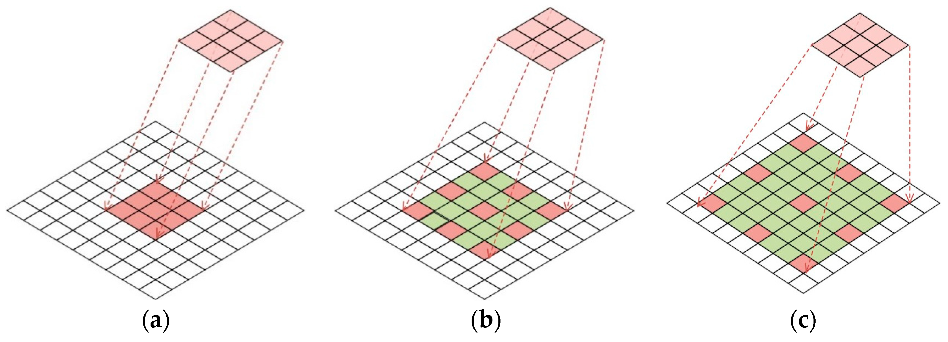
The dilated convolution [58] was originally developed in the wavelet decomposition algorithm [59] and known as a special convolution operator of Atrous convolution. The primary idea was to increase the receptive field by expanding the size of the convolution kernel without increasing the calculation. The receptive field size of dilated convolution varies depending on the number of intervals for the convolutional kernels, which are called the dilation rates. Thus, dilation convolution is effective for generating dense feature mappings between CNNs, which is extremely promising for pixel-level tasks. We provide a concise explanation of the dilation convolution in one dimension (1D) and two dimensions (2D).

For the 1D case, the input data, output data, filter, and filter size are represented by $x\left[i\right]$, $D\left[i\right]$, $f_D$, $k$, respectively. The dilated convolution is represented by the following Formula (1), where r denotes the dilated rate.

$$D\left[i\right]={\displaystyle \sum }_0^{k=1}{f}_D\times x\left[i+r\cdot k\right]$$

(1)

For the 2D case, the situation where $r$ is set to 1, 2, and 3, respectively is detailed in Figure 1. The fundamental concept behind dilated convolution is to insert (r − 1) zeros between adjacent convolution kernels of standard convolution. For example, considering that the convolution kernel is 3 × 3 and $r$ = 2, the receptive field of dilated convolution is 5 × 5. The green background represents the range of receptive fields.

3.2. Residual Convolution Network Structure

HSI classification performance can be greatly improved by utilizing CNN-based methods. However, once the network depth surpasses a certain extent, the phenomenon of gradient vanishing ensues which directly causes a deterioration of the network’s performance. The residual network (ResNet) [36] has the characteristic of being easy to optimize; thus, it can contribute to the prevention network degradation. Moreover, the residual blocks inside the ResNet can overcome the issue, of the over-deepening of the network, by skipping connections [36].

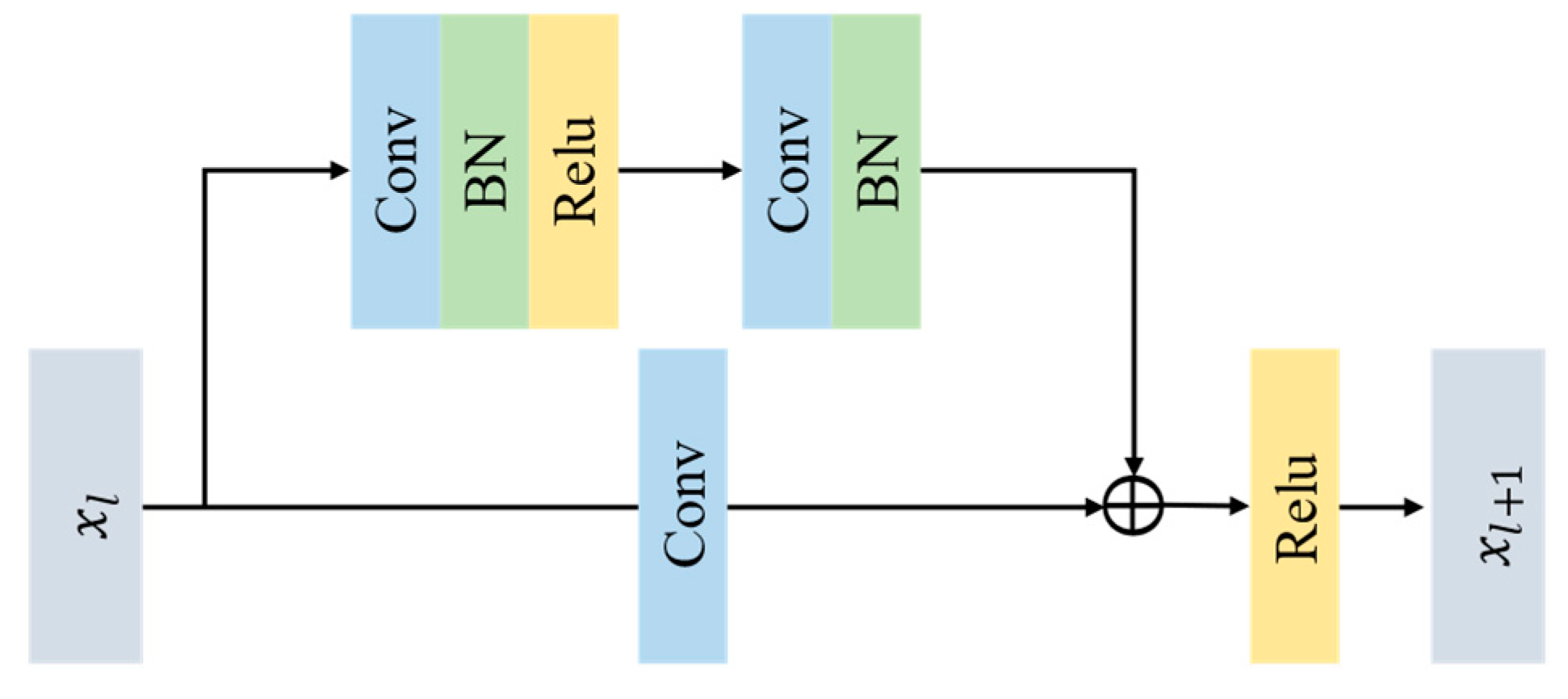
The ResNet is constructed by concatenating a set of residual blocks, and the detailed structure is shown in Figure 2. A residual block consists of a direct mapping $h\left(x_l\right)$ and a residual component $ℱ\left(x_l,W_l\right)$. The residual block can be defined by the following Equation (2), where $x_l$, $x_{l+1}$ represent the input and output of layer $l$, respectively. By using 1 × 1 convolution to resolve the different dimensionality of the feature maps of $x_l$ and $x_{l+1}$, the residual block can be expressed by Equation (3), where $h\left(x_l\right)=W_l^{\prime }x$, and 1 × 1 convolution is represented by $W_l^{\prime }$.

$$x_{l+1}=x_l+ℱ\left(x_l,W_l\right)$$

(2)

$$x_{l+1}=h\left(x_l\right)+ℱ\left(x_l,W_l\right)$$

(3)

3.3. Architecture of the Designed MHNA

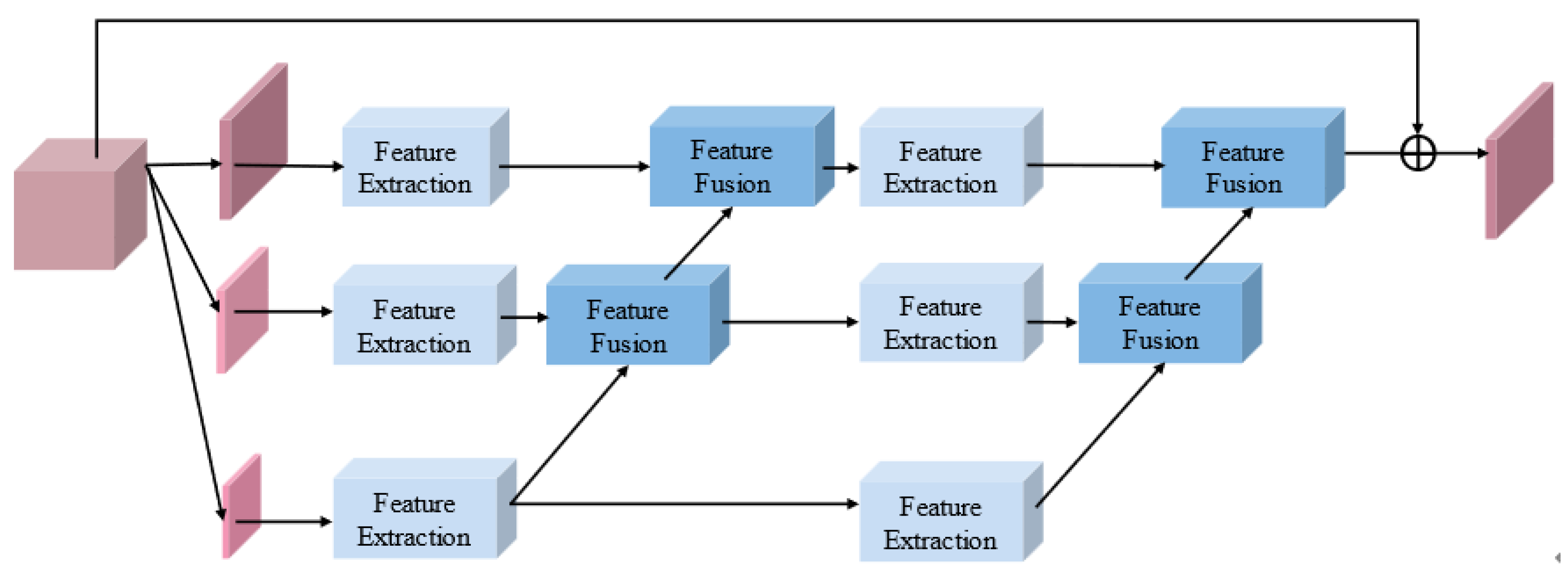
The structure of the MHNA mechanism is displayed in Figure 3, which is a parallel dual-branch architecture. The proposed approach has three components: a spectral-spatial feature extraction network, a spatial inverted pyramid network, and a classification network. The spectral-spatial feature extraction network contains three similar dilated convolution blocks combined with ResNet and a hybrid attention mechanism, which is applied to extract a substantial number of spectral signatures and a few spatial features. Additionally, the combination structure can effectively preserve and transmit the features obtained from the initial layers of the network. Next, the spatial inverted pyramid network is utilized to capture spatial features. The spatial inverted pyramid network includes two spatial inverted pyramid blocks. Each block consists of three down-sampling operations, four up-sampling operations, six feature extraction blocks, and four feature fusion blocks. Finally, the classification network includes a concatenate, a multi-head attention mechanism, a ReLu layer, and a fully connected layer, which are employed to obtain classification results. Among them, the concatenation operator is used to merge the features from different branches, and a multi-head attention mechanism can help the network pay attention to the information from different subspaces. The ReLu activation function introduces nonlinear properties into the model to improve network expressiveness. The fully connected layer is employed to generate the ultimate classification results.

3.4. Spatial-Spectral Feature Extraction Network

In the proposed network, a spectral-spatial feature extraction network is introduced to capture multiscale information from feature maps, as shown in Figure 4. It contains four similarly dilated convolutions combined with ResNet blocks (DR) and a hybrid attention mechanism. Additionally, the hybrid attention is located after the third DR block, which can greatly assist the fourth DR block to extract higher-level features of the network. The strategy can facilitate the network achieving a better performance in classification tasks. The architecture of the hybrid attention mechanism is depicted in Figure 5. Suppose $F\in {ℝ}^{H\times W\times C}$ is the input of attention, and multiplies it to a 1D channel attention tensor $A_{C }\in {ℝ}^{1\times 1\times C}$ to obtain the channel-refined feature $F^{\prime }$. $F^{\prime }$ is then divided into two groups, by the spatial attention submodule, which are called $F_1^{\prime }$, $F_2^{\prime }$. The two groups of features are produced their own 2D spatial attention tensors: $A_{s,1}\in {ℝ}^{H\times W\times 1}$, $A_{s,2}\in {ℝ}^{H\times W\times 1}$. By multiplying $A_{s,1}$, $A_{s,2}$ with $F_1^{\prime }$, $F_2^{\prime }$, respectively, a pair of spatial refined features are named $F_1^{″}$ and $F_2^{″}$, are generated. The process of a hybrid attention mechanism can be summarized by the following equations:

$$F^{\prime }=A_C\left(F\right) ⨂ F$$

(4)

$$F^{\prime }= F_1^{\prime }\oplus F_2^{\prime }$$

(5)

$$F_1^{″}=A_{s,1}\left(F_1^{\prime }\right)⨂ F_1^{\prime }$$

(6)

$$F_2^{″}=A_{s,2}\left(F_2^{\prime }\right)⨂ F_2^{\prime }$$

(7)

$$F^{″}=F_1^{″}\oplus F_2^{″}\oplus F$$

(8)

Next, we describe the network process of the spectral-spatial feature extraction network in detail on the Pavia Center. First, we randomly select a 3D patch cube (9 × 9 × 102) as the network’s original input to consider both spectral information around the central pixel and spatial information. The input data pass through a 3-D convolution with a convolution kernel of (1 × 1 × 1), filters of 8, stride of (1 × 1 × 1), and without padding. The size of the output feature map is (9 × 9 × 102, 8). Next, the outputs of 3-D convolution are fed into a cascade of DR blocks, which consists of dilated convolutions and residual convolutions. The dilated rate $d=2^n\left(n=0, \dots , 3\right)$ increases proportionally to the growth of n. The kernel size, stride, dilation rate, and filters of the first DR block are (1 × 1 × 3), (1 × 1 × 1), (1 × 1 × 1), and 16, respectively. The distinction between the other DR blocks and the first DR block is the number of filters and the dilated rate. The second block has filters of 32 with a dilation rate of (2, 2, 2), the third block has filters of 64 with a dilation rate of (4, 4, 4), and the last block has a filter of 16 with a dilation rate of (8, 8, 8). In addition, it should be emphasized that the convolution kernels of the parallel residual convolution in each block are (1 × 1 × 1), which are used to ensure that the elements of the feature fusion process are summed to obtain the same shape tensor. Finally, we get the feature map of (9 × 9, 16). The spectral-spatial feature extraction process is detailed in

Table 1. The details of spectral-spatial feature extraction network.

Name	Input	Operations	Kernel Size	Dilation	Filters	Output
Conv3D	(9 × 9 × 102, 1)	Conv3D	(1 × 1 × 1)	\	8	(9 × 9 × 102, 8)
DR Block 1	(9 × 9 × 102, 8)	ResConv	(1 × 1 × 1)	\	16	(9 × 9 × 102, 16)
	(9 × 9 × 102, 8)	Dilated Conv	(1 × 1 × 3)	(1, 1, 1)	16	(9 × 9 × 100, 16)
	(9 × 9 × 100, 16)	Dilated Conv	(1 × 1 × 3)	(1, 1, 1)	16	(9 × 9 × 98, 16)
	(9 × 9 × 102, 16)	Slice	\	\	\	(9 × 9 × 98, 16)
	(9 × 9 × 98, 16)/(9 × 9 × 98, 16)	Element-wise Sum	\	\	\	(9 × 9 × 98, 16)
DR Block 2	(9 × 9 × 98, 16)	ResConv	(1 × 1 × 1)	\	32	(9 × 9 × 98, 32)
	(9 × 9 × 98, 16)	Dilated Conv	(1 × 1 × 3)	(2, 2, 2)	32	(9 × 9 × 94, 32)
	(9 × 9 × 94, 32)	Dilated Conv	(1 × 1 × 3)	(2, 2, 2)	32	(9 × 9 × 90, 32)
	(9 × 9 × 98, 32)	Slice	\	\	\	(9 × 9 × 90, 32)
	(9 × 9 × 90, 32)/(9 × 9 × 90, 32)	Element-wise Sum	\	\	\	(9 × 9 × 90, 32)
DR Block 3	(9 × 9 × 90, 32)	ResConv	(1 × 1 × 1)	\	64	(9 × 9 × 90, 64)
	(9 × 9 × 90, 32)	Dilated Conv	(1 × 1 × 3)	(4, 4, 4)	64	(9 × 9 × 82, 64)
	(9 × 9 × 82, 64)	Dilated Conv	(1 × 1 × 3)	(4, 4, 4)	64	(9 × 9 × 74, 64)
	(9 × 9 × 90, 64)	Slice	\	\	\	(9 × 9 × 74, 64)
	(9 × 9 × 74, 64)/(9 × 9 × 74, 64)	Element-wise Sum	\	\	\	(9 × 9 × 74, 64)
Attention	(9 × 9 × 74, 64)	Hybrid Attention	\	\	\	(9 × 9 × 74, 64)
DR Block 4	(9 × 9 × 74, 64)	ResConv	(1 × 1 × 1)	\	16	(9 × 9 × 74, 16)
	(9 × 9 × 74, 64)	Dilated Conv	(1 × 1 × 3)	(8, 8, 8)	16	(9 × 9 × 58, 16)
	(9 × 9 × 58, 16)	Dilated Conv	(1 × 1 × 3)	(8, 8, 8)	16	(9 × 9 × 42, 16)
	(9 × 9 × 74, 16)	Slice	\	\	\	(9 × 9 × 42, 16)
	(9 × 9 × 42, 16)/(9 × 9 × 42, 16)	Element-wise Sum	\	\	\	(9 × 9 × 42, 16)
Sequential	(9 × 9 × 42, 16)	Reshape	\	\	\	(9 × 9, 672)
	(9 × 9, 672)	BN-Relu-Conv2D	(1 × 1)	\	16	(9 × 9, 16)

.

3.5. Spatial Inverted Pyramid Network

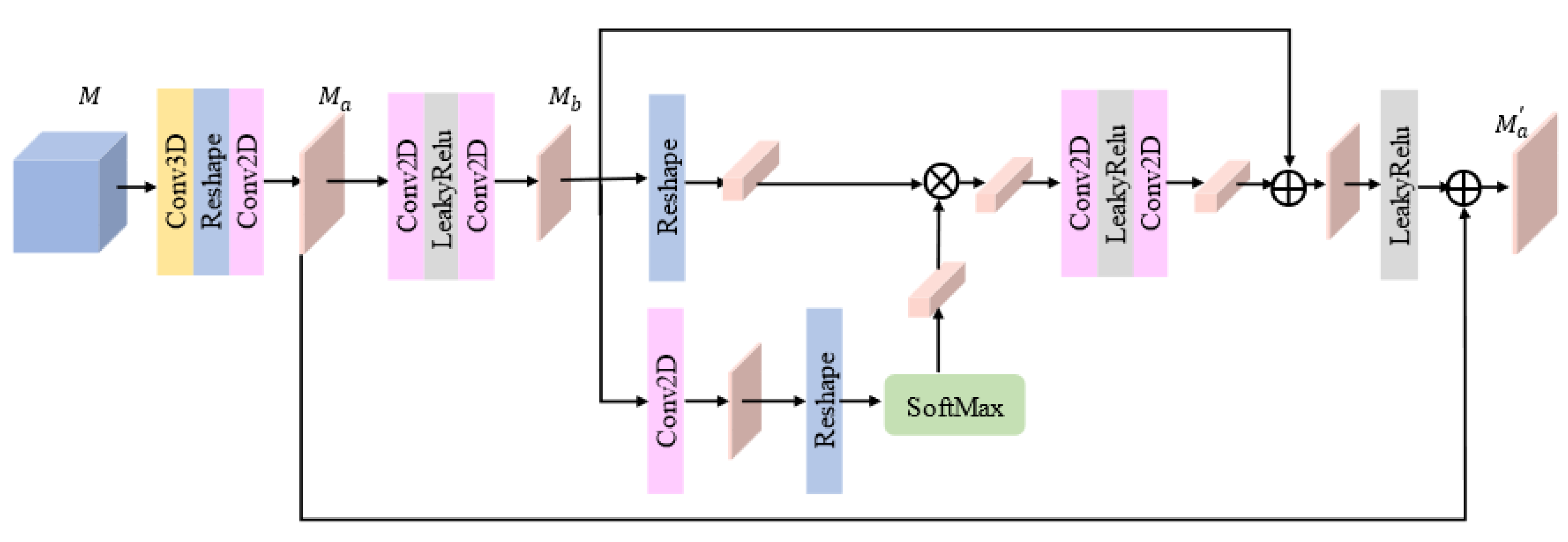
In the designed network, a spatial inverted pyramid network is applied to obtain multiscale spatial information from feature maps that are processed by PCA, as shown in Figure 6. The feature extraction block and the feature fusion block are essential components of the spatial inverted pyramid network. The spatial representations of the three different scales are first obtained by down-sampling operations and then fed into the feature extraction block separately. The objective of the feature extraction block is to capture spatial features in different scale streams, which can suppress less useful features and allow more informative ones to pass further. Then, the features from multiple scales are fused by the feature fusion blocks. Figure 7 illustrates the structure of the feature extraction block. Assuming $M \in {ℝ}^{H\times W\times C}$ as the original input after convolution and a reshaping operation to obtain $M_a \in {ℝ}^{H\times W}$, that is the beginning of the feature extraction block. The overall process of the feature extraction block is summarized as:

$$M_a=W_1\left(M\right)$$

(9)

$$M_b=W_{L_1}\left(M\right)$$

(10)

$$M_a^{\prime }=M_a+F_L[M_b+W_{L_2}\left({\sigma }_1\left(M_b\right)\times F_{SM}\left({\sigma }_2\left(W_2\left(M_b\right)\right)\right)\right)]$$

(11)

where $W_1$ denotes a set of operations, including 3-D and 2-D convolutions with kernel sizes (1 × 1 × 1), (2 × 2), and a reshape operator. $W_{L_1}$ represents 2-D convolutions with kernel size (3 × 3) and LeakyRelu. ${\sigma }_1$ and ${\sigma }_2$ are individual reshape operators, and a SoftMax operator is denoted by $F_{SM}$($·$).$W_{L_2}$ means a group of operations containing 2-D convolutions with kernel size (1 × 1) and LeakyRelu, $F_L$ stands for independent LeakyRelu operator. Finally, the output of the block is denoted by $M_a^{\prime }$.

The feature fusion block structure is illustrated in Figure 8. $L_1 \in {ℝ}^{H\times W}$ and $L_2 \in {ℝ}^{H\times W}$ are assumed to be the output from the feature extraction block and input of the feature fusion block, respectively. The fusion process can be represented as follows:

$$A_1=L_1\odot \left[W_s\left(W_L\left(GAP(L_1+L_2\right)\right))\right]$$

(12)

$$A_2=L_2\odot \left[W_s\left(W_L\left(GAP(L_1+L_2\right)\right))\right]$$

(13)

$$A=A_1+A_2$$

(14)

where GAP is the global average pooling. W_L represents a set of operations including a 2-D convolution using a kernel of size (1 × 1) and LeakyReLu operator. $W_s$ denotes a group operation containing a 2-D convolution applying a kernel of size (1 × 1) and SoftMax operators. $L_1$ and $L_2$ are element-wise products, obtaining $A_1$ and $A_2$, respectively, as a result of the above operation. $A \in {ℝ}^{H\times W}$ can be formulated as the ultimate output of the feature fusion block by Equation (14).

The details of the spatial inverted pyramid network are described on the Pavia Center dataset in

Table 2. The detail of spatial inverted pyramid network.

Name	Input	Operations	Kernel Size	Filter	Output
Input	(9 × 9 × 3, 1)	Conv3D	(1, 1, 1)	8	(9 × 9 × 3, 8)
	(9 × 9 × 3, 8)	Reshape	\	\	(9 × 9, 24)
	(9 × 9, 24)	Conv2D	(2, 2)	128	(8 × 8, 128)
Down-sampling	(8 × 8, 128)	\	\	\	(8 × 8, 128)
	(8 × 8, 128)	Down-sampling	(3, 3)/(3, 3)	192	(4 × 4, 192)
	(4 × 4, 128)	Down-sampling	(2, 2)/(2, 2)	288	(2 × 2, 288)
Up-sampling Feature Fusion	(2 × 2, 288)	Up-sampling	(2, 2)/(2, 2)	192	(4 × 4, 192)
	(4 × 4, 192)/(4 × 4, 192)	Feature Fusion	\	\	(4 × 4, 192)
Up-sampling	(4 × 4, 192)	Up-sampling	(3, 3)/(3, 3)	128	(8 × 8, 128)
Feature Fusion	(8 × 8, 128)/(8 × 8, 128)	Feature Fusion	\	\	(8 × 8, 128)
Output	(8 × 8, 128)	Conv2D	(1, 1)	128	(8 × 8, 128)
	(8 × 8, 128)/(8 × 8, 128)	Element-wise Sum	\	\	(8 × 8, 128)

. A 3D patch (9 × 9 × 3) is randomly selected as the network’s original input. The result of (8 × 8) is obtained by using a 3-D convolution with kernel size (1, 1, 1), a reshape operation, and a 2-D convolution using a kernel of size (2, 2). Subsequently, three different scales of spatial information, with sizes (8 × 8), (4 × 4), and (2 × 2), are generated by successive down-sampling operations. Then, the spatial features from different scale streams are extracted separately by the feature extraction block, and then are fused by the up-sampling operations and the feature fusion block.

3.6. Classification Network

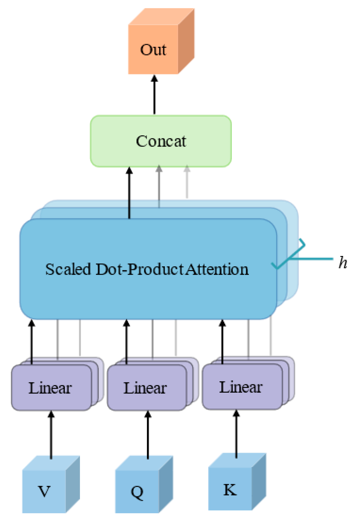
In the designed network, a classification network is employed to generate the classification results, which include a multi-head attention mechanism, ReLu, and fully connected layer. The multi-head attention mechanism can form multiple subspaces to optimize the features of different subspaces and balance the bias that may be overly focused on one. The structure of the multi-head attention is demonstrated in Figure 9. The scaled dot-product attention is an important operation within it. The following equation can be used to express it.

$$Attention\left(Q,K,V\right)=SoftMax\left(\frac{Q{K}^T}{\sqrt{d_k}}\right)V$$

(15)

With $Q$, $K$, and $V$ as input, the similarity of $Q$ and $V$ is obtained by SoftMax after the inner product of $Q$ and $K^T$. In addition, $\sqrt{d_k}$ is used as a scaling factor to prevent $Q{K}^T$ results from being too large, and the small gradient after SoftMax is not conducive to back propagation. The multi-head attention mechanism can be expressed by the following equations:

$$hea{d}_i=Attention\left(Q{W}_i^Q, K{W}_i^K,V{W}_i^V\right)$$

(16)

$$MultiHead \left(Q,K,V\right)=Concat\left(hea{d}_1, \dots , hea{d}_h\right)W^O$$

(17)

In (17), $Q$, $K$, and $V$ denote the query, key, and value, respectively. $h$ represents the number of heads; $hea{d}_i$ is the results of the $i$th head, and $W^O$ is the result transformation matrix. In (16), $W_i^Q$, $W_i^K$, and $W_i^v$ are, respectively, the query, key, and value transformation matrix of the $i$th head. $Attention$ can be described by (15). The detail of classification network is implemented in

Table 3. The detail of classification network.

Name	Input	Operations	Output
Classification	(9 × 9, 16)	Conv2D	(8 × 8, 16)
	(8 × 8, 16)/(8 × 8, 128)	Concatenate	(8 × 8, 144)
	(8 × 8, 144)	Multi-Head Attention	(8 × 8, 144)
	(8 × 8, 144)	Reshape	9216
	9216	ReLu-Dropout	256
	256	ReLu-Dropout	128
	128	ReLu	9

.

4. Experiment

4.1. Description of the Hyperspectral Datasets

In our experiments, the aim is to indicate the effectiveness of the designed approach. Five famous hyperspectral datasets from various imaging platforms are adopted. Detailed descriptions of the datasets are shown below:

Pavia Center dataset (PC): The PC dataset was acquired using the ROSIS sensor from Pavia Center, Italy. It comprises bands of 1096 × 715 pixels, and spectral reflectance bands in the range of 0.43–0.86 μm. The geometric resolution is 1.3 m. There are 13 noisy bands excluded, leaving 102 bands for classification to minimize the occurrence of mixed pixels. The PC’s ground truth consists of nine landcovers.

Salinas Valley (SA): The SA dataset was collected by the AVIRIS sensor. The spatial dimensions of SA are 512 × 217 and its resolutions is 3.7 m. The raw dataset of SA has 24 bands ranging from 0.4 to 2.5 μm. A total of 20 bands affected by water absorption are eliminated. As a result, we only use 204 bands for classification. The dataset comprises 16 types of landcover.

WHU-Hi-LongKou (LK): The LK dataset was obtained by the RSIDEA research group of Wuhan University. It comprises 550 × 400 pixels and 270 bands from 0.4 to 1.0 μm. The spatial resolution is approximately 0.463 m. The study site is an agricultural land space, which includes nine samples.

WHU-Hi-HongHu (HH): The HH dataset was captured by the RSIDEA research group of Wuhan University on 20 November 2017. The imagery size is 940 × 475 pixels, with 270 bands from 0.4 to 1.0 μm, and a spatial resolution of about 0.043 m. The dataset includes 22 classes, but 18 categories were selected from the original dataset in our experiment, and the processed image size is 331 × 330.

Huston (HO): The HO dataset was obtained by the ITERS CASI-1500 sensor in Houston, Texas, USA and its surrounding rural areas, with a spatial resolution of 2.5 m. Its data size is 349 × 1905 and it contains 144 bands in the 0.36 to 1.05 μm band range. There are 15 characteristic types in the study area, including roads, soil, trees, highways, etc.

4.2. Experiment Evaluation Indicators

Three evaluation indicators are applied to evaluate the classification performance of the designed approach in the article, namely, overall accuracy (OA), average accuracy (AA), and Kappa coefficient (Kappa) [60]. The confusion matrix is introduced to provide a more intuitive display of the three evaluation indexes mentioned above. In general, it is expressed in the matrix form of $\left(C_{n\times n}\right)$. In the confusion matrix, the prediction labels are represented by each column, and the actual labels are represented by each row. The matrix can be defined as follows:

$$C=\left[\begin{array}{ccc}{C}_{11}& \cdots & C_{1n}\\ ⋮& \ddots & ⋮\\ C_{n1}& \cdots & C_{nn}\end{array}\right]$$

(18)

In (18), the value of $n$ corresponds to the total number of categories, $C_{ij}$ represents the number of samples from class $i$ that are classified as class $j$, and $\sum _i^n{C}_{ij}$ and $\sum _j^n{C}_{ij}$ represent the total of the samples in each row and class. Therefore, OA, AA, and Kappa are described as follows:

$$OA=\frac{{\sum }_{i=1}^n{C}_{ii}}{{\sum }_i^n{\sum }_j^n{C}_{ij}}$$

(19)

$$AA=\frac{1}{n}\times {{\displaystyle \sum }}_{i=1}^n\frac{C_{ii}}{C_{ij}}$$

(20)

$$Kappa=\frac{OA-{\sum }_{i=1}^n\left({\sum }_i^n{C}_{ij}\times {\sum }_j^n{C}_{ij}\right)}{1-{\sum }_{i=1}^n\left({\sum }_i^n{C}_{ij}\times {\sum }_j^n{C}_{ij} \right)}$$

(21)

4.3. Experiment Setting

The experiment is performed on a workstation specifically designed for DL tasks; we use Intel(R) Xeon(R) CPU E5-26800 V4 processor. The clock frequency of CPU is 2.4 GHZ, the number of CPU cores is 14, and the cache size is 35,840 KB. At the same time, it also has 128 GB’s RAM and 6×NVIDIA GeForce RTX 2080Ti Super Graphics processing Unit with 12 GB of memory.

To verify the performance of our designed network, we choose ten methods for comparative experiments, including one the most classical ML method and nine advanced methods based on CNNs. The brief introduction to the comparative methods as follows:

(1)

SVM: From the perspective of classification, a SVM is a generalized classifier, which is evolved on the basis of a linear classifier by introducing a structural risk minimization principle, optimization theory and kernel function [61]. Each labeled sample, with a continuous spectral vector in the HSI, can be directly sent to the classifier without feature extraction and dimensionality reduction.

(2)

SSRN [37]: The primary idea of an SSRN is to capture features by stacking multiple spectral residual blocks and multiple spatial residual blocks. The spectral residual blocks used a 1 × 1 × 7 convolution kernel for feature extraction and dimensionality reduction. The spatial residual blocks use a 3 × 3 × 1 convolution kernel for spatial feature extraction. The classification accuracy is improved by adding batch normalization (BN) [62] and ReLu after each convolution layer.

(3)

FDSS [46]: The 1 × 1 × 7 and 3 × 3 × 7 convolution kernels are used to obtain spectral and spatial features, respectively. To improve the speed and prevent overfitting, the FDSSC uses a dynamic learning rate, a parameter correction linear unit (PRELU) [63], BN and dropout layer.

(4)

DBMA [53]: The network is composed of two branches, which extract spectral signatures and spatial features to reduce the interference between the two features. In addition, inspired by CBAM [64], a channel and a spatial attention mechanism are applied to the branches to improve the classification accuracy.

(5)

DMFN [49]: A two-branch network structure extracts spatial features through 2-D convolution and 2-D dense blocks. Additionally, it uses 3-D convolution and 3-D dense blocks to extract spectral features directly from the original data. Then, the two features are converged by 3-D convolutional blocks and 3-D dense blocks, which are different from the fusion of other networks.

(6)

PCIA [55]: It is a double-branch structure, which is implemented by pyramid 3D-CNN architecture, and the iterative attention mechanism is introduced into it. A new activation function, Mish, and an early stop are applied to improve the effective.

(7)

SSGCA [54]: The difference between SSGCA and DBMA is the attention mechanism, which refers to the GCNet [65].

(8)

MDANet [66]: The network is a multiscale three-branch dense connection attention network. Traditional 3-D convolutions are replaced with 3-D spectral convolution blocks and 3-D spatial convolution blocks.

(9)

MDBNet [67]: A multiscale dual-branch feature fusion network with attention mechanism is adopted in the network. It can extract pixel-level spatial and spatial features through a multiscale feature extraction block to enlarge the receptive field.

(10)

OSDN [56]: The combination of one-shot dense blocks and polarization attention mechanism comprises of two separate branches for feature extraction.

The designed approach is structured in an end-to-end manner. Specifically, parameters in the network can be trained and the network is able to learn features in HSIs and perform feature extraction and classification tasks. Details of the MHNA implementation are summarized in Algorithm 1. To ensure the impartiality of the experiment, the same hyperparameters are applied to all methods, and the Adam optimizer [68] is used to update for 200 training epochs. The initial learning rate is set to 0.001 and the cosine annealing [69] method is employed to dynamically adjust the learning rate each 15 epochs. In addition, an early-stopping mechanism is added to terminate the training process and enter the testing phase if the validation loss does not decrease for 20 consecutive epochs. The input of the HSI cube patch size is 9 × 9, and the batch size is 64. Additionally, the original input of the spatial inverted pyramid network reduces the dimension to 3 by using PCA.

Table 4. Landcover categories and dataset division in the PC dataset.

Class	Category	Total	Train	Validation	Test
C1	Water	824	8	8	808
C2	Trees	820	8	8	804
C3	Asphalt	816	8	8	800
C4	Self-blocking bricks	808	8	8	792
C5	Bitumen	808	8	8	792
C6	Tiles	1260	13	13	1234
C7	Shadows	476	5	5	466
C8	Meadows	824	8	8	808
C9	Bare Soil	820	8	8	804
	Total	7456	74	74	7308

,

Table 5. Landcover categories and dataset division in the SA dataset.

Class	Category	Total	Train	Validation	Test
C1	Weeds-1	2009	40	40	1929
C2	Weeds-2	3726	75	75	3576
C3	Fallow	1976	40	40	1896
C4	Fallow-P	1394	28	28	1338
C5	Fallow-S	2678	54	54	2570
C6	Stubble	3959	79	79	3801
C7	Celery	3597	72	72	3453
C8	Grapes	11,271	225	225	10,821
C9	Soil	6203	124	124	5955
C10	Corn	3278	66	66	3146
C11	Lettuce-4wk	1068	21	21	1026
C12	Lettuce-5wk	1927	39	39	1849
C13	Lettuce-6wk	916	18	18	880
C14	Lettuce-7wk	1070	21	21	1028
C15	Vineyard-U	7268	145	145	6978
C16	Vineyard-T	1807	36	36	1735
	Total	54,129	1083	1083	51,963

,

Table 6. Landcover categories and dataset division in the LK dataset.

Class	Category	Total	Train	Validation	Test
C1	Corn	34,511	345	345	33,821
C2	Cotton	8374	84	84	8206
C3	Sesame	3031	30	30	2971
C4	Broad-leaf soybean	63,212	632	632	61,948
C5	Narrow-leaf soybean	4151	42	42	4067
C6	Rice	11,854	119	119	11,616
C7	Water	67,056	671	671	65,714
C8	Roads and houses	7124	71	71	6982
C9	Mixed weed	5229	52	52	5125
	Total	204,542	2046	2046	200,450

,

Table 7. Landcover categories and dataset division in the HH dataset.

Class	Category	Total	Train	Validation	Test
C1	Red roof	3320	33	33	3254
C2	Road	1609	16	16	1577
C3	Bare soil	20,574	205	205	20,164
C4	Cotton	1792	17	17	1758
C5	Cotton firewood	27,964	279	279	27,406
C6	Rape	8993	89	89	8815
C7	Chinese cabbage	4054	40	40	3974
C8	Pak choi	2375	23	23	2329
C9	Cabbage	939	9	9	921
C10	Tuber mustard	5847	58	58	5731
C11	Brassica parachinensis	1233	12	12	1209
C12	Brassica chinensis	5348	53	53	5242
C13	Small Brassica chinensis	4307	43	43	4221
C14	Lactuca sativa	1002	10	10	982
C15	Celtuce	1517	15	15	1487
C16	Film covered lettuce	1436	14	14	1408
C17	White radish	973	9	9	955
C18	Garlic sprout	2037	20	20	1997
	Total	95,320	945	945	93,430

and

Table 8. Landcover categories and dataset division in the HO dataset.

Class	Category	Total	Train	Validation	Test
C1	Healthy grass	1251	12	12	1215
C2	Stressed grass	1254	12	12	1228
C3	Synthetic grass	697	6	6	683
C4	Trees	1244	12	12	1220
C5	Soil	1242	12	12	1218
C6	Water	325	3	3	229
C7	Residential	1268	12	12	1242
C8	Commercial	1244	12	12	1220
C9	Road	1252	12	12	1228
C10	Highway	1227	12	12	1203
C11	Railway	1235	12	12	1211
C12	Parking1	1233	12	12	1209
C13	Parking2	469	4	4	459
C14	Tennis Court	428	4	4	420
C15	Running Track	660	6	6	646
	Total	15,029	143	143	14,743

provide the quantity of the training sets, validation sets, and test sets on the five datasets.

Algorithm 1 Structure of the designed MHNA

Input:

(1) Unprocessed HSI by PCA: H with b bands

(2) Processed HSI by PCA: P with p bands

Step 1: H and P are normalized and divided into training test, validation test, and test set.

Step 2: A w $\times$ w $\times$ b patch, extracted around each pixel of the dimension-unreduced HSI, is considered the spectral-spatial features.

Step 3: A w $\times$ w $\times$ p patch, extracted around each pixel of the dimension-reduced HSI, is considered the spatial features.

Step 4: The samples of the training test are fed into the network and optimized using the Adam optimizer. The initial learning rate is set 0.001. It is adjusted dynamically every 15 epochs.

Step 5: The classification of the total HSI is achieved by inputting the corresponding spectral and spatial features to the network.

Step 6: The two-dimensional matrix records labels of the HSI.

Output: Prediction classification map

4.4. Experiment Results

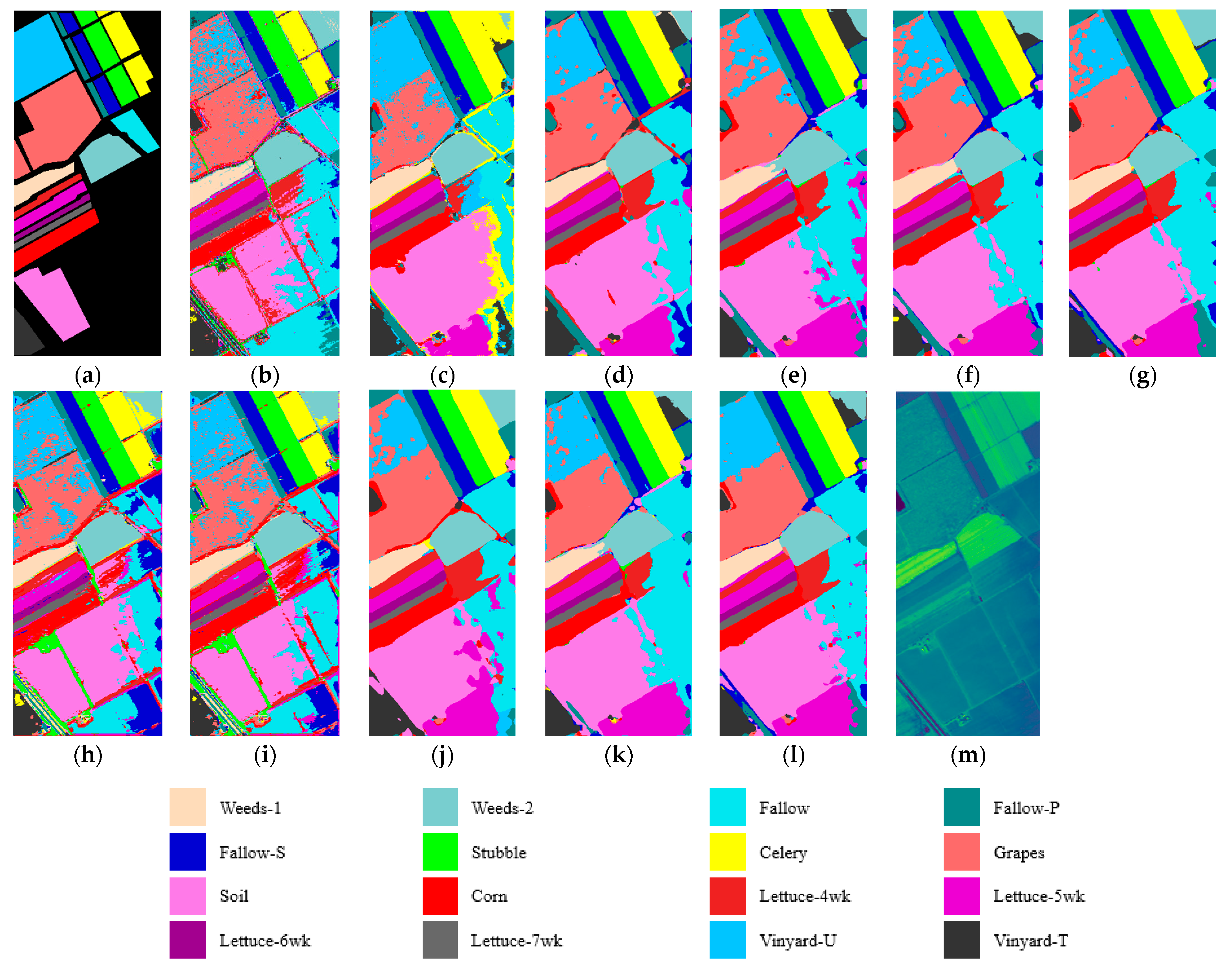
We first analyze the classification performance of the various approaches on the SA dataset in

Table 9. Classification accuracies of various approaches on the SA dataset (The best results are highlighted in bold).

Class	Color	SVM	SSRN	FDSS	DBMA	DMFN	PCIA	MDAN	MDBN	SSGC	OSDN	MHNA
C1		95.15	100.0	100.0	100.0	99.19	100.0	98.95	99.92	100.0	100.0	100.0
C2		99.45	99.91	100.0	100.0	99.83	100.0	99.19	99.80	100.0	98.59	99.81
C3		99.48	100.0	97.74	100.0	98.45	100.0	91.30	98.71	100.0	97.73	100.0
C4		98.83	95.72	98.04	91.13	95.91	100.0	99.83	94.00	98.95	99.62	99.55
C5		93.18	100.0	97.99	99.27	98.54	99.92	85.09	99.24	99.49	99.45	99.57
C6		99.66	99.73	100.0	99.78	99.97	100.0	99.82	98.23	100.0	100.0	100.0
C7		99.03	99.53	99.94	100.0	99.51	100.0	95.38	99.16	99.04	99.24	99.94
C8		86.14	96.36	95.11	94.64	88.00	84.57	86.12	97.72	83.56	92.70	95.51
C9		96.12	99.71	99.26	100.0	99.81	99.89	98.31	100.0	100.0	100.0	99.61
C10		88.37	99.90	97.33	90.54	94.15	99.65	94.16	99.86	98.99	99.67	97.71
C11		93.20	100.0	93.98	99.90	97.62	100.0	87.50	100.0	99.61	100.0	99.02
C12		99.26	99.94	99.67	99.78	99.89	99.94	95.39	99.92	100.0	99.94	99.03
C13		98.00	90.16	97.99	99.65	100.0	100.0	93.16	100.0	99.77	99.31	99.66
C14		93.53	99.41	99.70	97.85	97.83	99.02	98.50	98.38	100.0	95.85	98.34
C15		49.26	77.90	92.17	83.55	82.49	99.09	72.51	71.52	99.03	93.78	92.66
C16		94.07	100.0	98.50	100.0	98.12	100.0	98.85	97.20	100.0	100.0	99.72
OA (%)		87.94	95.24	97.23	95.54	94.29	96.07	90.52	93.84	95.64	97.24	97.74
AA (%)		92.67	97.39	97.96	97.25	96.83	98.88	93.38	97.10	98.65	98.49	98.76
Kappa×100		86.54	94.71	96.91	95.04	93.64	95.61	89.46	93.17	95.13	96.93	97.49
Parameters (M)		\	0.40	1.54	0.50	3.92	0.53	0.51	0.49	0.42	0.10	4.32

. The best OA, AA, and Kappa results are highlighted in bold. The proposed approach is compared with the SVM, SSRN, FDSSC, DBMA, DMFN, PCIA, MDAN, MDBN, SSGCA, and OSDN approaches. The proposed MHNA improves OA by 9.77%, 2.50%, 0.51%, 2.20%, 3.45%, 1.67%, 7.22%, 3.90%, 2.10%, and 0.50% more than the above methods, respectively. It is because the spectral-spatial feature extraction network and the spatial inverted pyramid network are applied to jointly extract spectral and spatial features. Additionally, losing the multiscale information is prevented by using residual convolution in the spectral-spatial feature extraction network. The OA of the SVM is lower compared to that of DL-based methods, because the SVM only utilizes the spectral signatures of the HSI. The MDAN and MDBN have lower OA than other DL-based methods. This indicates that it is difficult to target the characteristics of the hyperspectral dataset and to extract discriminative features on the SA dataset. The PCIA network, based on a pyramid structure, achieves the highest AA among all methods, reaching 98.88%. It shows that the pyramid structure has an extremely high potential for feature extraction. It can be observed that the SSRN and FDSS achieve lower OAs than the proposed MHNA and OSDN. This is because SSRNs and FDSSs extract spectral and spatial features through two consecutive convolutional blocks. Additionally, the input of the spatial block is derived from the spectral block, resulting in the loss of some spatial information. The DBMA and DMFN are dual-branch networks, while the DBMA has better OA than the DMFN. The distinction between the DMFN and DBMA lies in the absence of the attention mechanism in the DMFN. This suggests that attention mechanisms have a significant impact on the network. Meanwhile, the number of parameters for all approaches is reported in Table 9. It can be concluded that the number of parameters obtained by the SVM method can be ignored. Because the SVM is an ML method, it contains an extremely small number of parameters. Other methods are based on DL, which include both single input (SSRN, FDSS, DBMA, PCIA, MDAN, MDBA, and OSDN) and dual input (DMFN and MHNA) approaches. It is clear that dual input approaches implement a larger number of parameters than others. The MHNA mechanism received the highest OA. The classification result maps of all methods are displayed in Figure 10. We can note that the proposed MHNA is the closest to the real image (Figure 10a). And it can be clearly seen in Figure 10b,e–j that a large number of the C8 (Grapes) is mistaken in C15 (Vineyard-U). It indicates that it is difficult to distinguish C8 and C15 on the SA dataset. From the classification map of Figure 10l, achieved by the proposed MHNA, it is worth noting that there is a small number of samples that are misclassified. The experimental results indicate that the designed approach is more effective than other approaches for classification tasks.

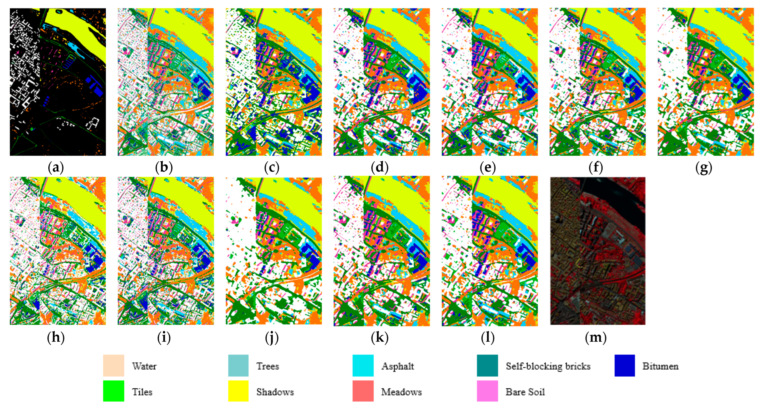
The PC is a dataset of urban center landscapes, which contains nine landcovers. All methods, including SVM, achieve satisfactory classification results, as displayed in

Table 10. Classification accuracies of various approaches on the PC dataset (The best results are highlighted in bold).

Number	Color	SVM	SSRN	FDSS	DBMA	DMFN	PCIA	MDAN	MDBN	SSGC	OSDN	MHNA
C1		99.95	99.53	99.97	99.99	99.97	100.0	99.98	99.97	99.99	99.98	100.0
C2		90.71	99.46	98.35	98.02	97.66	98.65	96.91	96.49	97.72	98.89	97.13
C3		84.54	99.85	91.09	90.68	89.87	89.36	90.20	93.26	90.35	83.34	96.47
C4		86.87	84.32	90.34	90.51	79.04	96.87	78.77	85.89	89.08	89.38	96.31
C5		91.96	98.85	95.16	95.41	91.48	97.99	99.40	98.03	99.10	99.57	98.54
C6		93.96	96.96	98.42	97.34	96.02	93.71	93.84	96.63	93.98	97.31	99.52
C7		84.54	82.44	99.48	99.01	98.55	99.57	95.96	97.02	99.93	99.98	96.49
C8		99.1	99.91	99.84	99.81	99.65	99.62	97.67	99.40	99.37	99.92	99.80
C9		99.93	99.85	99.24	98.67	98.07	99.81	99.96	99.96	98.77	97.20	99.75
OA (%)		97.1	97.96	99.13	99.02	98.41	99.00	97.88	98.76	98.81	99.05	99.38
AA (%)		92.4	94.57	96.51	96.60	94.48	97.29	94.74	96.29	96.48	96.17	98.22
Kappa×100		96.2	97.10	98.55	98.62	97.75	98.58	96.99	98.25	98.32	98.66	99.13
Parameters (M)		\	0.21	0.34	0.21	4.06	0.22	0.49	0.49	0.21	0.05	3.33

. Parameters obtained by MHNA are less than DMFN. As can be observed, the designed MHNA has an outstanding performance and achieves the highest OA, AA, and Kappa. In particular, the MHNA achieves 100% on C1 (Water). However, SVM, DMFN, PCIA, and OSDN achieve an OA of less than 90% on C3 (Asphalt). And FDSS, DBMA, MDAN, and SSGC achieve an OA of less than 92% on C3. A similar phenomenon is observed for C4 (Self-blocking bricks); it can be seen that most approaches achieve an OA lower than 90%. This indicates that it is a challenge to classify C3 and C4 accurately. Conversely, the proposed MHNA achieves OAs of more than 96% on C3 and C4. The classification maps in the PC dataset are exhibited in Figure 11. It is apparent that the landcover contours and boundaries are smoother and clearer on Figure 11l, which is obtained by the proposed approach.

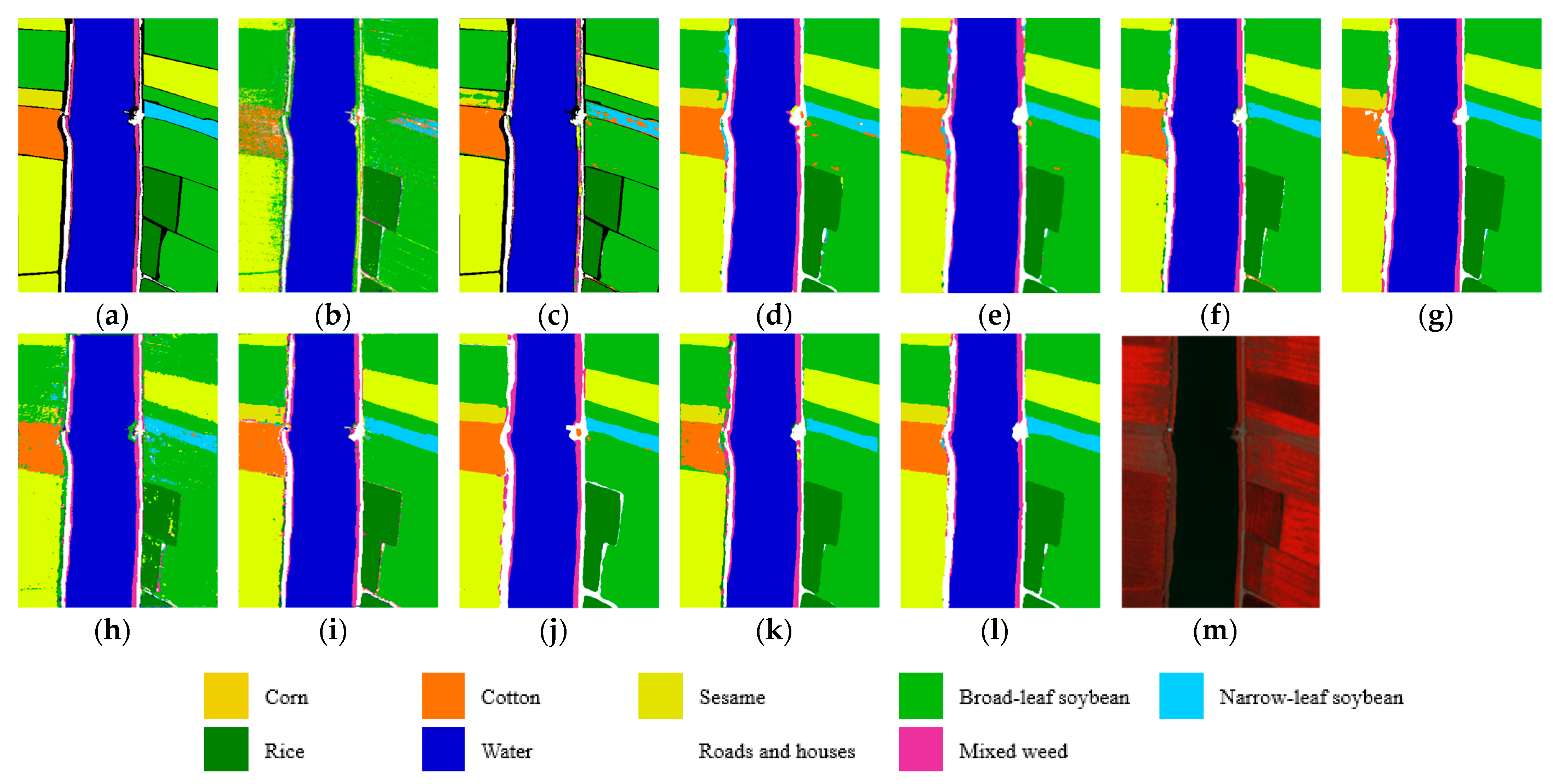
There are nine landcovers in the LK dataset, which includes numerous samples. The precise experimental results are displayed in

Table 11. Classification accuracies of various approaches on the LK dataset (The best results are highlighted in bold).

Number	Color	SVM	SSRN	FDSS	DBMA	DMFN	PCIA	MDAN	MDBN	SSGC	OSDN	MHNA
C1		98.28	97.78	99.40	99.91	99.79	99.93	97.41	99.77	99.93	99.44	99.69
C2		76.61	84.70	92.93	99.34	97.36	99.97	96.12	99.13	96.70	99.69	98.82
C3		76.52	99.77	100.0	100.0	96.45	98.97	50.27	92.53	99.62	100.0	100.0
C4		96.52	96.57	99.40	97.67	99.24	99.55	94.83	99.59	99.47	96.99	99.54
C5		61.37	100.0	91.85	95.84	99.46	95.61	79.16	95.47	99.86	99.15	98.38
C6		97.93	97.58	99.74	99.92	99.94	98.44	95.85	99.45	100.0	98.39	99.46
C7		99.99	99.92	99.99	99.93	99.93	99.95	99.66	99.88	99.99	99.94	99.98
C8		82.58	91.09	88.82	93.30	98.50	92.89	95.80	96.65	87.36	98.01	96.51
C9		67.30	99.96	88.53	96.35	93.33	91.56	90.01	93.96	83.07	93.30	93.60
OA (%)		90.77	97.30	98.52	98.78	99.30	99.16	96.12	99.25	98.70	98.57	99.40
AA (%)		84.12	96.37	95.63	98.03	98.22	97.43	88.79	97.38	96.22	98.32	98.44
Kappa×100		93.38	96.43	98.05	98.40	99.09	98.90	94.89	99.02	98.30	98.12	99.21
Parameters (M)		\	0.47	2.22	0.50	3.24	0.53	0.49	0.52	0.51	0.10	3.61

. It can be easily seen that the OA of the SVM is 90.77%. For specific classes, the accuracy is less than 70% of the SVM, such as with C5 (Narrow leaf soybean) and C9 (Mixed weed). The SSRN, FDSS, and MDNA use spectral and spatial features, and these approaches outperform SVM in terms of classification accuracy. The performance of these methods (the DBMA, DMFN, PCIA, MDBN, SSGC, OSDN, and MHNA) is relatively stable, and satisfactory results have been obtained. It proves that the structure of dual-branch networks is more stable. It is remarkable that the designed MHNA achieved the largest number of parameters while also obtaining the highest OA, AA, and Kappa. The maps displaying the full-factor classification are presented in Figure 12. It is evident that the salt-pepper noise presents in Figure 12b, which is achieved by the SVM. Conversely, the classification maps of the DL-based method are smoother. This suggests that the smoothness of the classification maps can be enhanced by extracting spatial features in DL-based methods. As shown in Figure 12a,l, the classification map obtained by MHNA is the most approximate to the real landcovers.

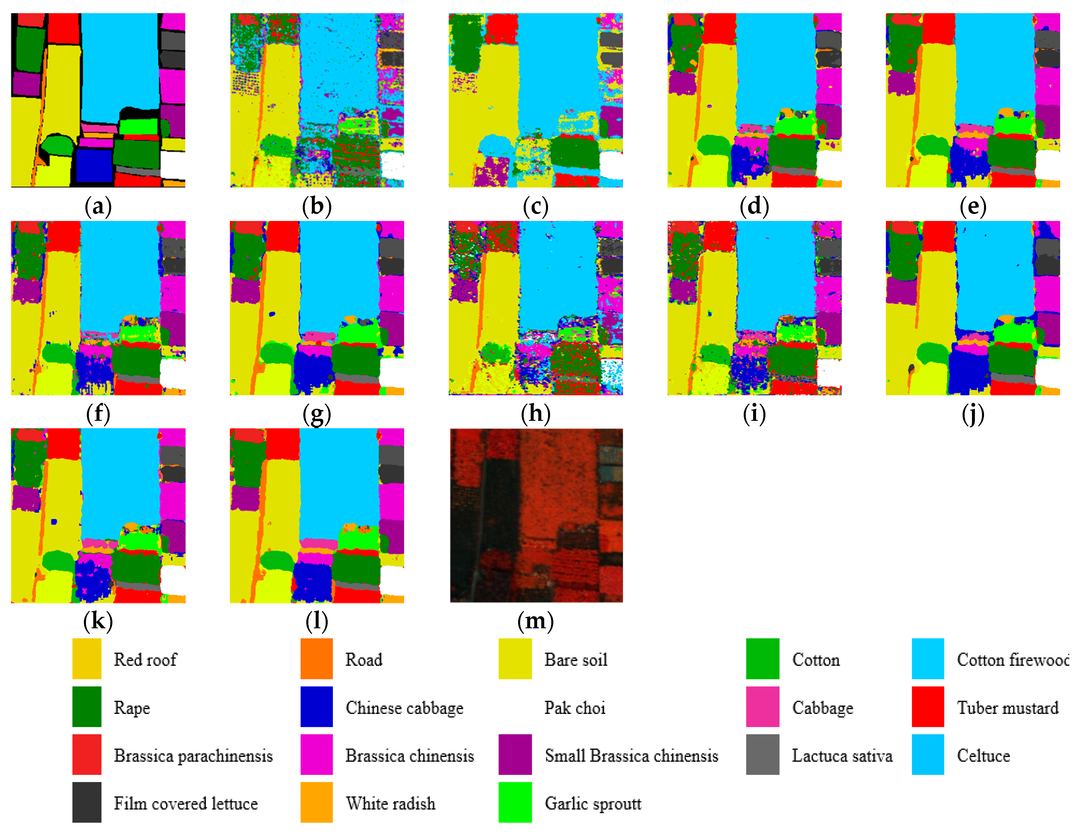
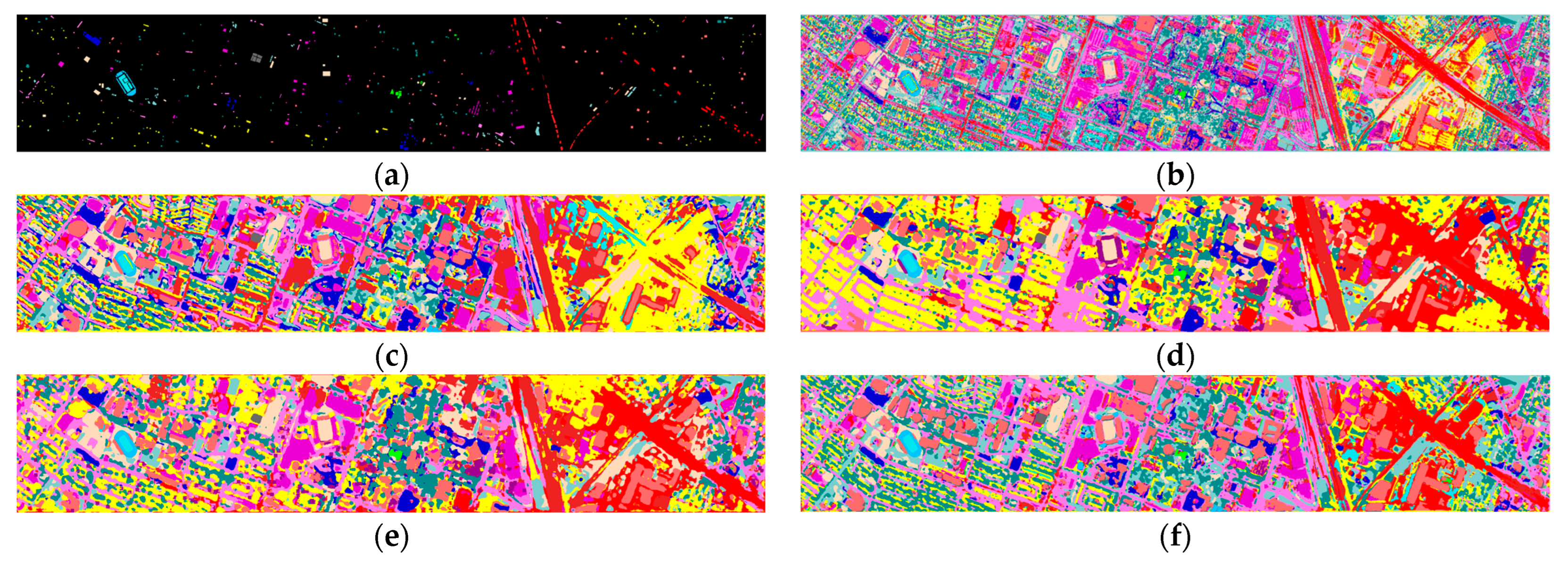
Additionally, to assess the effectiveness of the introduced MHNA, a high spatial resolution HSI dataset named HH is selected. From

Table 12. Classification accuracies of various approaches on the HH dataset (The best results are highlighted in bold).

Number	Color	SVM	SSRN	FDSS	DBMA	DMFN	PCIA	MDAN	MDBN	SSGC	OSDN	MHNA
C1		69.01	94.35	94.89	99.65	97.38	98.01	66.32	76.74	98.33	97.87	98.59
C2		70.59	84.21	85.55	78.19	93.26	88.21	79.76	86.08	98.77	83.35	94.47
C3		93.98	94.88	95.22	95.11	94.98	98.91	86.73	96.19	96.71	97.80	99.18
C4		89.48	99.52	95.23	96.29	96.90	97.25	86.11	80.93	98.24	98.80	98.88
C5		96.52	99.33	99.19	98.67	98.66	99.27	90.88	99.43	100.0	99.79	99.80
C6		63.53	81.75	92.35	95.77	92.12	98.09	62.36	91.98	98.19	95.42	97.89
C7		17.56	93.28	92.81	86.21	80.46	84.02	45.23	74.66	66.35	88.46	98.46
C8		88.44	97.03	99.82	98.44	97.88	99.44	64.83	96.40	99.82	99.78	99.11
C9		6.67	86.71	97.79	83.73	95.81	91.66	65.85	70.24	98.40	93.04	92.42
C10		20.21	98.30	91.89	94.07	94.66	96.10	54.21	87.57	96.33	96.78	97.68
C11		49.29	99.13	99.21	99.61	98.69	97.55	92.86	60.60	100.0	99.70	98.10
C12		46.27	96.03	88.42	90.38	91.08	98.20	75.60	93.41	98.10	90.01	98.48
C13		40.44	98.17	95.66	98.61	96.55	97.59	83.30	93.43	99.19	98.54	98.37
C14		55.82	96.78	97.45	92.88	94.46	94.55	77.51	54.81	93.23	98.58	92.02
C15		73.42	85.16	85.85	90.97	84.58	97.49	80.64	87.63	100.0	96.70	96.48
C16		61.59	91.51	77.52	91.94	92.80	94.95	70.34	66.88	82.20	91.64	97.98
C17		0	97.99	80.98	75.63	88.76	98.33	42.52	48.18	84.34	89.14	89.49
C18		63.34	86.42	91.03	91.98	87.68	74.85	64.69	68.28	82.08	91.75	97.92
OA (%)		73.24	94.59	94.78	95.20	94.82	96.83	79.34	90.94	95.51	96.78	98.59
AA (%)		55.92	93.36	92.27	92.12	93.15	94.69	71.65	79.63	93.90	94.90	96.96
Kappa×100		67.55	93.51	93.81	94.30	93.85	96.25	75.20	89.27	94.68	96.19	98.33
Parameters (M)		\	0.47	2.22	0.51	4.37	0.54	0.50	0.49	0.51	0.11	3.75

, maximum and minimum parameters are achieved by the OSDN and the DMFN, respectively. The SVM based only on spectral signatures achieves the lowest OA of 73.24%. The difficulty of classifying various landcovers, utilizing spectral signatures exclusively on the HH dataset, is highlighted by the results. Contrasting the classification accuracy across different categories, the results indicate that some categories—such as C2 (Road), C7 (Chinese cabbage), C9 (Cabbage), C17 (White radish), and C18 (Garlic sprout)—are difficult to classify precisely using SVM, DBMA, MDAN, and MDBN. The proposed MHNA, as a dual-branch multiscale network, achieves more stable classification results compared to other methods. From Figure 13l, C3 (Bare soil) is almost completely correctly classified by the proposed method. On the contrary, the boundary between C2 and C3 is unclear in Figure 13b–d,h,j,k. However, it can be seen that there are small patches of misclassification in Figure 13l. These may be caused by using the dilated convolution injecting holes to expand the receptive field, which leads to discontinuity in information extraction.

The HO dataset contains 15 categories, such as roads, soils, and trees. The classification accuracies and parameter number of the eleven approaches are detailed in

Table 13. Classification accuracies of various approaches on the HO dataset (The best results are highlighted in bold).

Class	Color	SVM	SSRN	FDSS	DBMA	DMFN	PCIA	MDAN	MDBN	SSGC	OSDN	MHNA
C1		85.11	84.47	90.08	79.96	95.59	85.97	92.07	97.75	96.24	79.29	82.75
C2		65.12	99.90	99.52	99.49	87.34	96.79	95.68	98.51	90.53	93.95	97.75
C3		99.41	79.47	100.0	100.0	90.55	100.0	89.26	91.04	100.0	100.0	100.0
C4		80.81	98.36	97.95	94.88	87.85	93.81	94.29	92.31	96.22	92.28	99.64
C5		89.37	85.71	95.52	92.97	97.32	88.26	92.30	98.74	87.50	93.69	95.59
C6		67.44	97.85	100.0	99.61	98.75	100.0	82.16	91.00	100.0	87.39	99.27
C7		56.43	53.68	82.78	78.11	92.22	85.21	50.19	66.39	92.44	86.99	75.45
C8		62.08	99.62	89.72	91.52	96.19	97.97	58.38	52.34	75.92	90.36	93.44
C9		38.92	78.87	70.87	89.63	85.51	80.28	75.27	77.31	64.07	76.38	86.88
C10		55.68	94.97	71.85	87.96	75.44	65.51	78.98	77.93	80.27	91.52	84.99
C11		79.20	40.45	91.78	86.93	78.23	90.84	70.39	67.48	92.86	86.53	91.81
C12		74.74	53.58	91.39	86.83	88.88	81.74	66.55	69.98	94.61	93.88	88.72
C13		87.61	100.0	71.25	82.12	96.69	84.70	16.03	11.43	60.47	80.12	97.64
C14		92.67	94.53	95.62	100.0	97.10	95.45	80.73	80.63	100.0	100.0	92.58
C15		73.29	98.58	99.84	98.18	94.96	100.0	97.33	98.74	96.14	95.43	97.83
OA (%)		68.58	73.32	88.33	89.62	89.13	87.41	77.10	79.37	87.09	88.94	90.43
AA (%)		73.86	84.00	89.88	91.21	90.91	89.77	75.97	78.09	88.48	89.85	92.29
Kappa×100		66.03	71.09	87.39	88.77	88.24	86.38	75.23	77.67	86.04	88.05	89.65
Parameters (M)		\	0.27	0.65	0.28	3.52	0.31	0.49	0.49	0.28	0.06	3.31

. The HO dataset includes a smaller number of training samples than others. Therefore, it is extremely challenging to classify categories precisely under this condition. The lowest classification results are still achieved by the SVM. The phenomenon is enough to demonstrate the importance of spatial information of HSIs. Spectral and spatial characteristics are simultaneously exploited by the MHNA, which obtains the highest levels of OA, AA and Kappa. All the classification maps are presented in Figure 14. It can be clearly seen that there are plenty of misclassified samples in all maps.

5. Discussion

5.1. Discussion of Various Spatial Patch Sizes

We now discuss the influence of the patch size on the classification accuracy of the MHNA. An appropriate patch size is selected to help the network extract useful spatial information and to reduce the waste of computer resources. The large spatial patch may contain more information, but it also contains redundant information. In contrast, the small spatial patch contains insufficient spatial information, which is not conducive to extracting discriminative features to distinguish between similar categories. As shown in Figure 15, we summarize the OAs for various spatial patch sizes, which range from 5 × 5 to 13 × 13 with a 4-pixel interval. The reason for the 4-pixel interval is the continuous down-sampling operations applied in the spatial inverted network. It can be seen clearly that the classification accuracy varies with the spatial patch size. When the spatial patch size is 9 × 9, the highest OA is achieved on the five datasets. The experimental results show that the spatial patch sizes are not proportionate to the classification accuracy. In conclusion, the selected 9 × 9 patch sizes are applied in five datasets in our experiments.

5.2. Analysis of the Impact of Varying Training Sample Proportions

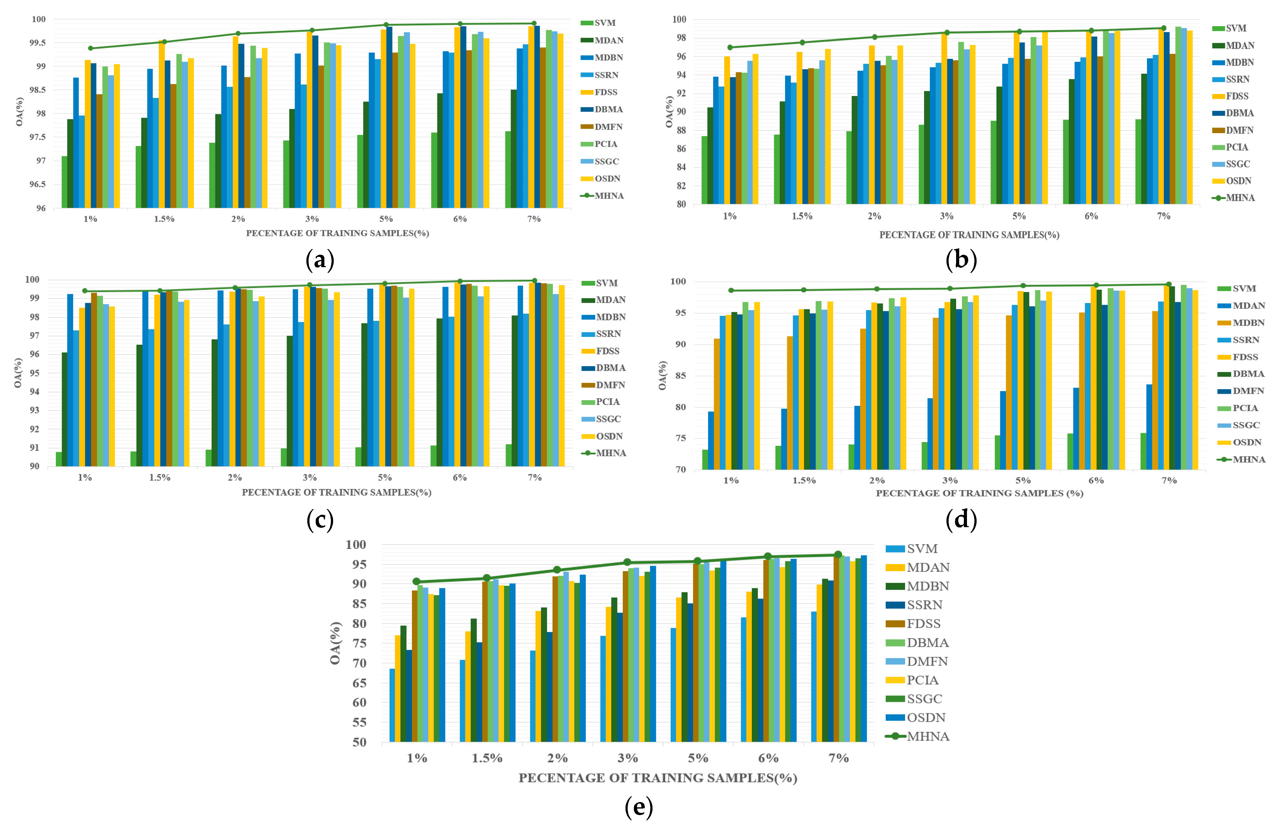
The classification performance among all methods is discussed on five datasets with various proportions of training samples in this section. It is well known that DL-based approaches require numerous labeled samples to extract discriminative features that are used for classification tasks. However, obtaining labeled samples is considered to be a time-consuming and laborious process. Consequently, the number of training samples is crucial for the learning process of DL-based methods. In order to compare and clearly analyze the performance of the designed approach in classification and the competitors with various proportions of training samples, we randomly chose 1%, 1.5%, 2%, 3%, 5%, 6%, and 7% of labeled training samples from each dataset. As shown in Figure 16, it is evident that the classification accuracy varies with the proportion of training samples. Additionally, the larger the number of training samples selected, the higher the OAs obtained by all methods. In contrast to other classification algorithms, the classification accuracies of FDSS, OSDN, and the proposed MHNA grow more slowly, especially in the LK and HH datasets, which are shown in Figure 16c,d. It demonstrates that these approaches can capture discriminative features to improve classification performance, even when limited training data is available. Satisfactory OAs are achieved by all methods when the proportion is 7% of the labeled training data. The accomplishment of the proposed method is extremely competitive. It is attributed to the important role played by the spectral-spatial pyramid network in our approach. By leveraging two networks, we can extract spectral-spatial features and abundant spatial features, which are crucial for classification tasks. In conclusion, the experimental results confirm the effectiveness of the designed MHNA in HSI classification tasks with limited training data.

5.3. Ablation Analysis

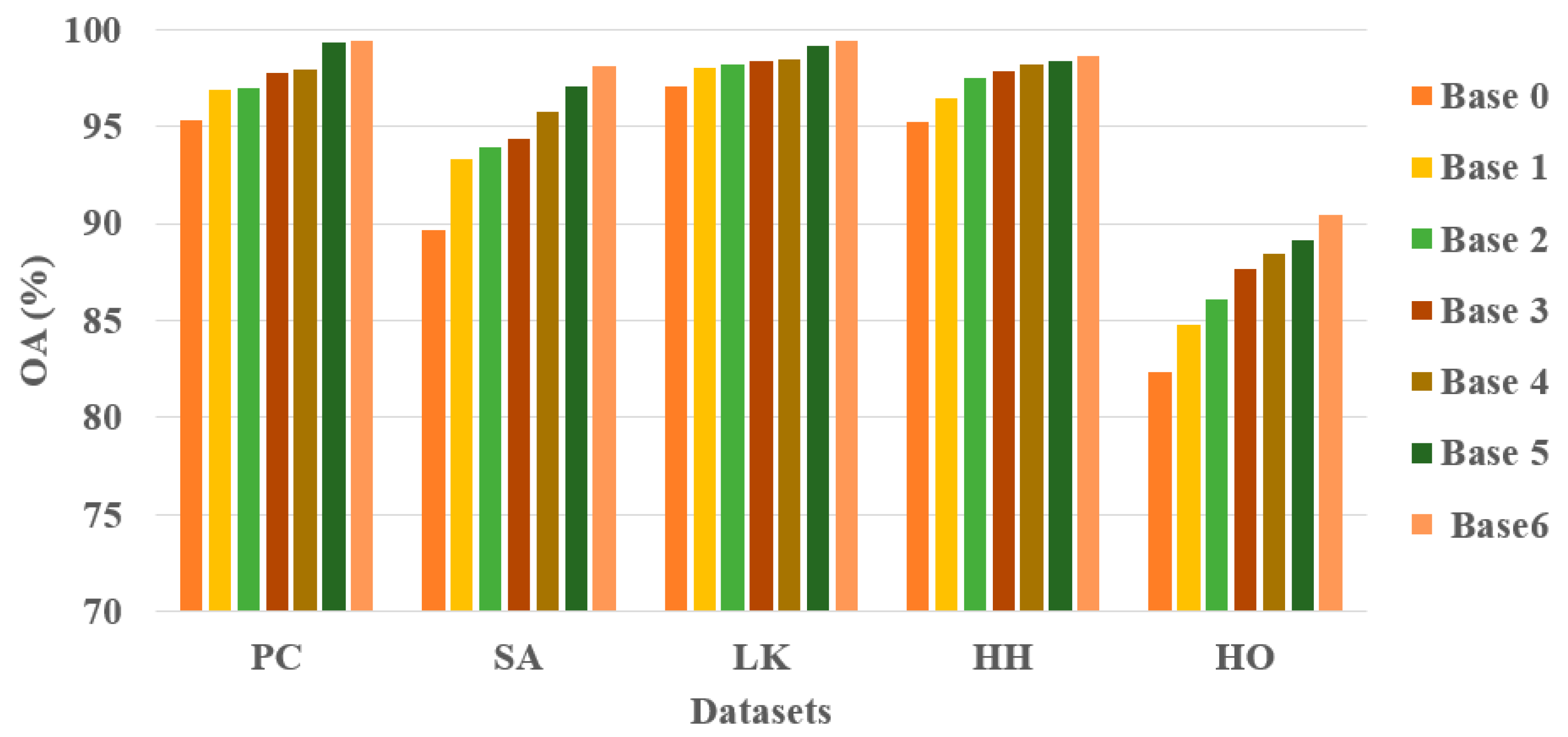
Six ablation experiments are conducted to analyze the performance of the modules in the designed method on five datasets. Additionally, dilated convolution, combined with ResNet blocks (DR), a hybrid attention mechanism, a multi-head attention mechanism, and spatial inverted pyramid blocks, are contained in six individual models. For the sake of fairness in comparison, the same hyperparameters and training samples selected are used in ablation experiments, which are introduced in Section 4.3. First, we apply the model that contains only one spatial inverted pyramid block (SIPB), and a DR block as the baseline named Base 0. The model of Base 1 consists of one SIPB and two DR blocks. One SIPB and three DR blocks are included in Base 2 and Base 3. In addition, hybrid attention is embedded in Base 3, and Base 4 is composed of 4 DR blocks, one SIPB, and hybrid attention. Base 0, Base 1, Base 2, Base 3, and Base 4 are employed to verify the capability of multiscale network feature extraction and the interaction with hybrid attention. The difference between Base 5 and Base 4 is that Base 5 incorporates two SIPBs to verify the validity of the SIPB. In the proposed MHNA, there are two separate attention mechanisms: hybrid attention and multi-head attention. Base 6 is based on Base 5 with the addition of multi-headed attention to verify whether this attention mechanism contributes to the network’s classification capability. The usage of modules is presented in

Table 14. The Usage of modules.

Name	DR1	DR2	DR3	DR4	SIPB1	SIPB2	Hybrid Attention	Multi-Head Attention
Base 0	√				√
Base 1	√	√			√
Base 2	√	√	√		√
Base 3	√	√	√		√		√
Base 4	√	√	√	√	√		√
Base 5	√	√	√	√	√	√	√
Base 6	√	√	√	√	√	√	√	√

. The results of the ablation experiments are illustrated in Figure 17. It is clear that the classification accuracies on five datasets are improved to varying degrees by incorporating the DB blocks, SIPBs, and the two attention mechanisms. In detail, the OAs of the Base 1 include two DR blocks and are improved by 1.54%, 3.68%, 0.93%, 1.20%, and 2.45% compared to Base 0, which contains one DR block on five different datasets. Compared to Base 1, which contains two DR blocks, the OAs of Base 2 that includes three DR blocks increased by 0.93% to 3.68%. Experimental results show that a multiscale network can capture image features more comprehensively to improve network performance. Compared with Base 3 and Base 5 without attention, Base 4 with hybrid attention and Base 6 with multi-head attention both show improved OAs on five datasets to varying degrees. This suggests that attention mechanisms play an essential role in the MHNA. The OAs of the Base 5 include two SIPBs, which are improved by 1.38%, 1.32%, 0.69%, 0.15%, and 0.65%, respectively, compared to Base 4 contains, which one SIPB. This indicates that the spatial inverted pyramid network can contribute to the proposed MHNA to capture more informative features. It can be observed that the best classification accuracy obtained by Base 6 includes four DR blocks, two SIPBs, and attention mechanisms on five HSI datasets, which indicates the usefulness of the modules applied in the proposed approach.

5.4. Visualization of Attention Mechanisms on a PC Dataset

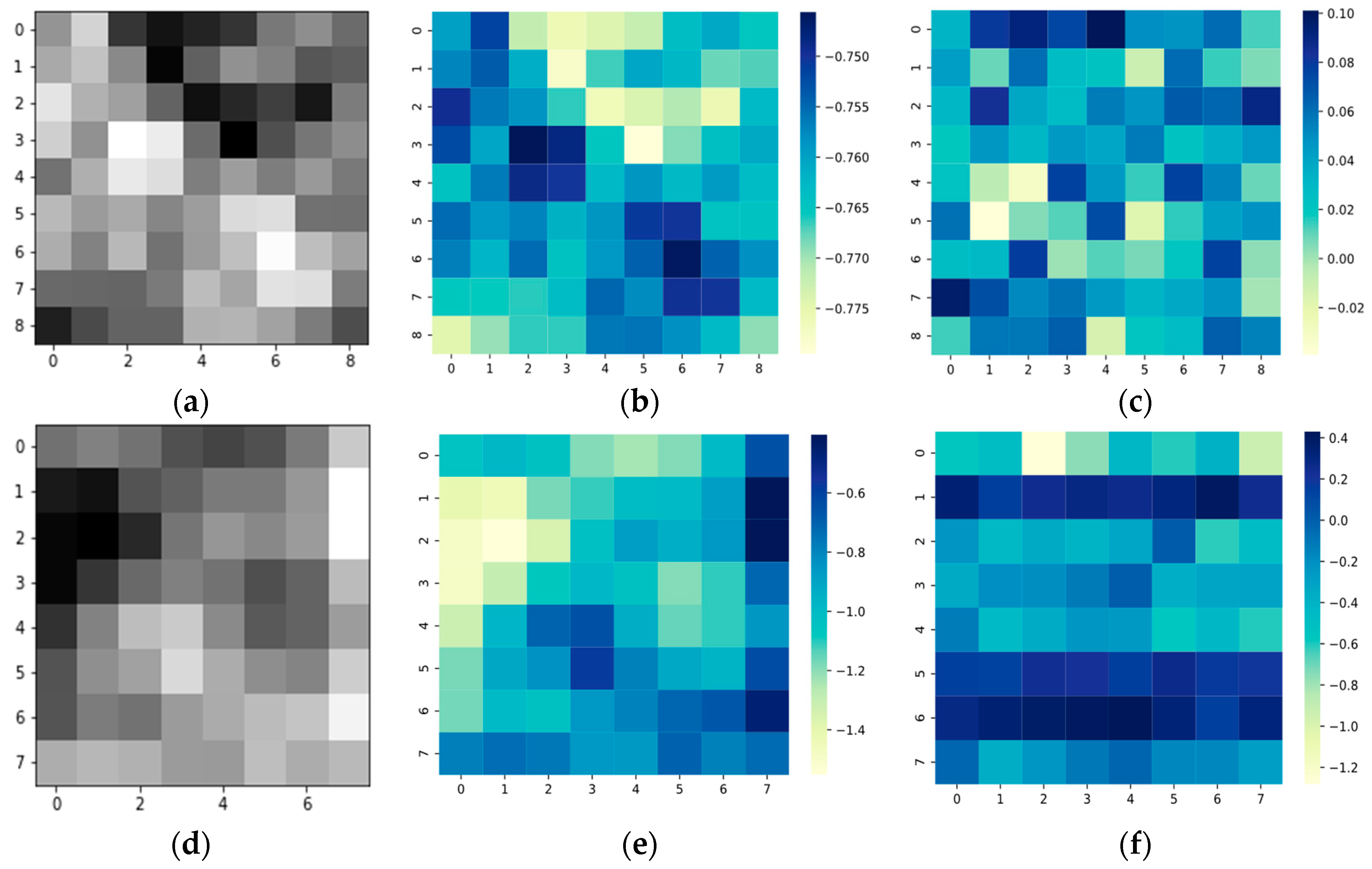
In the section, attention mechanisms are visualized as heat maps to further verify their facilitating effect on the designed MHNA. The PC dataset is selected as an example, and the visualized results are displayed in Figure 18. According to the input size of the network, a feature map of 9 × 9 pixels is taken out. It is clear from Figure 18a that the black pixels are background information and do not belong to any one category. While HSIs contain the spectral information of each pixel in a certain band range, not every pixel is meaningful for the classification task. Specifically, the labeled species are essential for the classification. The attention mechanism plays a crucial role in helping the network identify useful features and in improving its classification ability. To see it more directly, the weight matrices as heat maps. Figure 18b,c represent the heat maps before and after the hybrid attention is applied, respectively, and the darker the color of the pixel in the heat map, the higher its weight. Comparing Figure 18b,c with (a), it is clear that the weight corresponding to the key information in Figure 18b is lower, which is unfavorable for the subsequent classification task. However, the weights of the parts containing the landcovers in Figure 18b are increased by the hybrid attention. Therefore, the addition of a hybrid attention is beneficial for spectral-spatial feature extraction network. The multi-head attention is located after the fusion of two different features. As can be seen in Figure 18d, which is a grayscale image before the multi-head attention. In Figure 18e, the values of the weight matrix vary widely, and the one processed by multi-head attention is displayed in Figure 18f. We can see that the attention weight matrix has less variation in values and does not focus excessively on one part. Consequently, the multi-head attention prevents the network from focusing too much on one part, increasing the generalization ability of the model. In summary, both attention mechanisms, located at different locations, can contribute to the network and help in the subsequent classification tasks.

5.5. Analysis of the Classification Performance of the Proposed MHNA Visualized by t-SNE

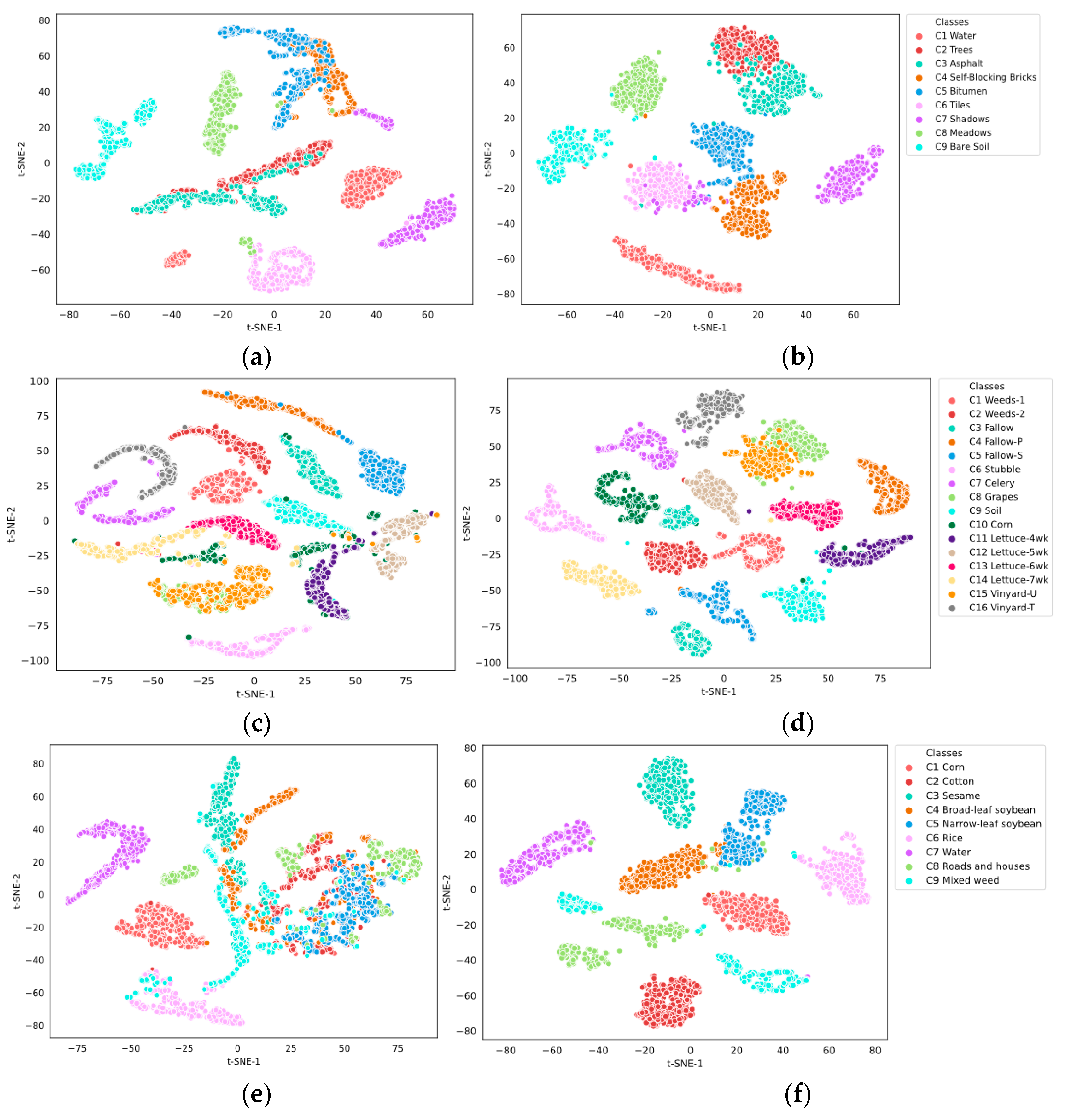
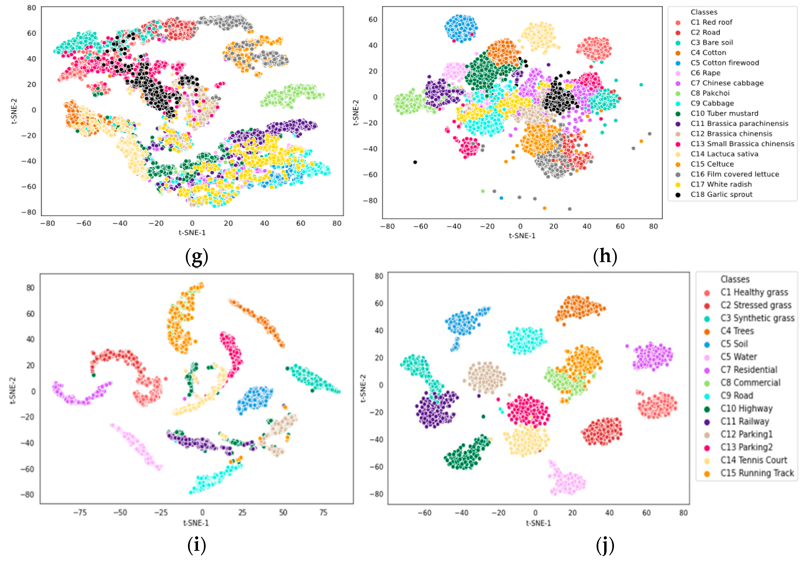
T-distributed stochastic neighbor embedding (t-SNE) was jointly developed by Laurens van Maaten and Geoffrey Hinton in 2008 [70]. t-SNE is considered as an effective technique for visualizing high-dimensional data. Specifically, it can preserve the local features of the datasets by mapping data points from high-dimensional to low-dimensional space, which more clearly demonstrates intra-class proximity and inter-class dissimilarity. In this section, the sample distributions of the five original datasets and the sample distributions, after being processed by the MHNA, are mapped to the 2D spaces. To make the results clearer, 400 samples from each class on the PC dataset, 260 samples from each class on the HO dataset, and 500 samples from each on the other three datasets are selected. In order to evaluate the classification performance of the designed MHNA, the same number of samples are selected from the test sets of the network.

The visualization results on five HSI datasets are displayed in Figure 19. The results of the sample distribution of the PC dataset are illustrated in Figure 17. From Figure 19a, it is evident that C2 (Trees) overlaps with C3 (Asphalt) and C1 (Water) overlaps with C5 (Bitumen). It indicates that there is a high degree of similarity between overlapping different categories and it is difficult to distinguish them. The above problem is alleviated by the proposed MHNA, as shown in Figure 19b. It suggests that the proposed method has the ability to extract discriminative features for distinguishing similar classes. The visualization results from the SA dataset, the LK dataset and the HO dataset are shown in Figure 19c,e,i. As we can see, there are some samples of the same category with scattered distribution, such as C10 (Corn) on the SA dataset; C1 (Corn), C2 (Cotton), and C8 (Roads and houses) on the LK dataset; and C10 (Highway) and C15 (Running Track) on HO dataset. Figure 19d,f,j are visualization results processed by MHNA; the distance between samples of the same category is significantly reduced. This demonstrates that the proposed MHNA can effectively reduce intra-class intervals to aggregate the samples in the same category. Finally, the HH dataset contains a substantial number of samples of various categories, as shown in Figure 19g. All kinds of samples are mixed together except C8 (Pak choi), which has no obvious boundaries. The results, after being processed by the network, are exhibited in Figure 19h, and it can be seen that the samples in the same category are grouped together and clear boundaries appear between the different classes. This demonstrates that the MHNA can effectively increase the inter-class distance, which can contribute to the enhancement the classification accuracy. In summary, the MHNA contains a spectral-spatial feature extraction network, a spatial inverted pyramid network, and attention mechanisms, which can help the network to capture extensive spectral and spatial features.

5.6. Discussion of Training Times and Testing Times

In this section, the training times and testing times of all approaches are discussed and analyzed with regard to five HSI datasets. A detailed report is displayed in

Table 15. Training times and testing times of various models in five datasets.

	Model	SVM	SSRN	FDSS	DBMA	DMFN	PCIA	MDAN	MDBN	SSGC	OSDN	MHNA
PC	Train (s)	27.63	69.60	103.94	156.31	391.81	155.18	979.75	160.88	103.70	72.49	120.27
	Test (s)	1.23	27.45	24.92	34.07	45.50	44.54	439.62	71.63	41.46	41.33	51.42
SA	Train (s)	25.21	210.14	386.69	180.68	130.92	224.46	3562.48	302.06	183.92	128.53	92.33
	Test (s)	1.44	17.04	21.01	21.28	26.27	26.60	802.50	52.35	29.06	30.29	33.71
LK	Train (s)	61.62	453.45	290.62	106.71	250.96	144.33	2752.99	313.72	239.29	117.39	303.13
	Test (s)	6.42	69.96	138.49	95.32	115.02	118.89	2257.85	254.36	174.03	76.49	123.66
HH	Train (s)	20.03	127.12	71.96	55.39	109.90	58.59	8232.32	129.47	75.54	54.96	100.85
	Test (s)	3.47	57.48	53.26	40.73	49.72	55.71	1007.42	117.33	62.42	36.59	41.36
HO	Train (s)	3.31	15.51	37.62	94.04	42.50	26.03	167.65	104.77	69.15	32.92	50.31
	Test (s)	0.18	2.49	2.23	23.92	10.38	5.52	19.19	29.13	13.66	6.47	14.42

. It is apparent that the shortest training times and testing times are achieved by the SVM; this is because there is a minimal number of parameters in the SVM. The training times obtained by the OSDN are the shortest of all DL-based methods on the LK and HH datasets. Because of the improved dense connection, named one-shot aggregation is implemented in the OSDN, and the training speed of the FDSS network, which used the dense connection, is slower than the OSDN within five datasets. This shows that one-shot aggregation is more efficient than the dense connection in the network, which is beneficial to reduce the training times. The SSRN and the proposed MHNA receive the shortest training times on the PC, HO, and SA datasets, separately, because the technique called ResNet is used in the SSRN and the proposed MHNA. This indicates that residual connections have the ability to shorten the training process. The dual-branch structure of these methods (the DBMA, PCIA, and SSGC), combined with attention mechanisms, have a similar computational efficiency. The MDAN achieves the longest training times and testing times of all approaches within the five datasets, because the MDAN is a three-branch network that contains several dense connections. This suggests that the lengths of training times and testing times are associated with the structure and technology applied in the network. From Table 15, it is clearly demonstrated that the training times and testing times obtained by the proposed method are not the shortest. This may have been caused by the dimensionality reduction technique used only in the spatial inverted pyramid network, and because several feature extraction blocks and feature fusion blocks are applied to the spatial inverted pyramid network. Although these structures slightly increase the complexity of the proposed network, the increase in classification performance is still worthwhile.

6. Conclusions

A multiscale hybrid network with attention mechanisms is proposed in this article, which is capable of extracting spectral and spatial features from HSI data concurrently. It contains three components: a spectral-spatial feature extraction network, a spatial inverted pyramid network, and a classification network. The multiscale hybrid network is employed to increase the receptive field and preserve the shallow features of the low-level layers in the spectral-spatial feature extraction subnetwork. The hybrid attention is used to focus on useful features and suppress useless features. Furthermore, a spatial inverted pyramid network is applied for extracting spatial features, which allows more informative information to pass further. Finally, the multi-head attention in the classification network provides multiple subspaces and helps the network to pay attention to the information from different subspaces, compared with ten approaches on five different datasets. This indicates that the MHNA is extremely competitive with the limited labeled samples. However, compared to traditional methods, it remains a time-consuming and laborious model. In the future, we plan to concentrate on simplifying the network architecture while maintaining classification accuracy.

References

1. Weng, Q. Remote sensing of impervious surfaces in the urban areas: Requirements, methods, and trends. Remote Sens. Environ. 2012, 117, 34–49. [Google Scholar] [CrossRef]
2. Heiden, U.; Segl, K.; Roessner, S.; Kaufmann, H. Determination of robust spectral features for identification of urban surface materials in hyperspectral remote sensing data. Remote Sens. Environ. 2007, 111, 537–552. [Google Scholar] [CrossRef]
3. Jiao, Q.; Zhang, B.; Liu, J.; Liu, L. A novel two-step method for winter wheat-leaf chlorophyll content estimation using a hyperspectral vegetation index. Int. J. Remote Sens. 2014, 35, 7363–7375. [Google Scholar] [CrossRef]
4. Zhang, B.; Shen, Q.; Li, J.; Zhang, H.; Wu, D. Retrieval of three kinds of representative water quality parameters of Lake Taihu from hyperspectral remote sensing data. J. Lake Sci. 2009, 21, 182–192. [Google Scholar]
5. Nasrabadi, N.M. Hyperspectral target detection: An overview of current and future challenges. IEEE Signal Process. Mag. 2013, 31, 34–44. [Google Scholar] [CrossRef]
6. Li, S.; Song, W.; Fang, L.; Chen, Y.; Ghamisi, P.; Benediktsson, J.A. Deep learning for hyperspectral image classification: An overview. IEEE Trans. Geosci. Remote Sens. 2019, 57, 6690–6709. [Google Scholar] [CrossRef]
7. Xue, J.; Zhao, Y.; Bu, Y.; Chan, J.C.-W.; Kong, S.G. When Laplacian scale mixture meets three-layer transform: A parametric tensor sparsity for tensor completion. IEEE Trans. Cybern. 2022, 52, 13887–13901. [Google Scholar] [CrossRef]
8. Xue, J.; Zhao, Y.; Huang, S.; Liao, W.; Chan, J.C.-W.; Kong, S.G. Multilayer sparsity-based tensor decomposition for low-rank tensor completion. IEEE Trans. Neural Netw. Learn. Syst. 2021, 33, 6916–6930. [Google Scholar] [CrossRef]
9. Du, B.; Zhang, L. Target detection based on a dynamic subspace. Pattern Recognit. 2014, 47, 344–358. [Google Scholar] [CrossRef]
10. Ma, L.; Crawford, M.M.; Tian, J. Local Manifold Learning-Based k-Nearest-Neighbor for Hyperspectral Image Classification. IEEE Trans. Geosci. Remote Sens. 2010, 48, 4099–4109. [Google Scholar] [CrossRef]
11. Kuo, B.-C.; Ho, H.-H.; Li, C.-H.; Hung, C.-C.; Taur, J.-S. A kernel-based feature selection method for SVM with RBF kernel for hyperspectral image classification. IEEE J. Sel. Top. Appl. Earth Obs. Remote Sens. 2013, 7, 317–326. [Google Scholar] [CrossRef]
12. Kang, X.; Xiang, X.; Li, S.; Benediktsson, J.A. PCA-based edge-preserving features for hyperspectral image classification. IEEE Trans. Geosci. Remote Sens. 2017, 55, 7140–7151. [Google Scholar] [CrossRef]
13. Bruce, L.M.; Koger, C.H.; Li, J. Dimensionality reduction of hyperspectral data using discrete wavelet transform feature extraction. IEEE Trans. Geosci. Remote Sens. 2002, 40, 2331–2338. [Google Scholar] [CrossRef]
14. Huang, S.; Zhang, H.; Xue, J.; Pižurica, A. Heterogeneous regularization-based tensor subspace clustering for hyperspectral band selection. IEEE Trans. Neural Netw. Learn. Syst. 2022, 1–15. [Google Scholar] [CrossRef] [PubMed]
15. Yu, H.; Gao, L.; Liao, W.; Zhang, B.; Zhuang, L.; Song, M.; Chanussot, J. Global spatial and local spectral similarity-based manifold learning group sparse representation for hyperspectral imagery classification. IEEE Trans. Geosci. Remote Sens. 2019, 58, 3043–3056. [Google Scholar] [CrossRef]
16. Jia, S.; Wu, K.; Zhu, J.; Jia, X. Spectral–spatial Gabor surface feature fusion approach for hyperspectral imagery classification. IEEE Trans. Geosci. Remote Sens. 2018, 57, 1142–1154. [Google Scholar] [CrossRef]
17. Jia, S.; Hu, J.; Zhu, J.; Jia, X.; Li, Q. Three-dimensional local binary patterns for hyperspectral imagery classification. IEEE Trans. Geosci. Remote Sens. 2017, 55, 2399–2413. [Google Scholar] [CrossRef]
18. Hong, D.; Gao, L.; Yao, J.; Zhang, B.; Plaza, A.; Chanussot, J. Graph convolutional networks for hyperspectral image classification. IEEE Trans. Geosci. Remote Sens. 2020, 59, 5966–5978. [Google Scholar] [CrossRef]
19. Hinton, G.E.; Salakhutdinov, R.R. Reducing the dimensionality of data with neural networks. Science 2006, 313, 504–507. [Google Scholar] [CrossRef]
20. Lateef, F.; Ruichek, Y. Survey on semantic segmentation using deep learning techniques. Neurocomputing 2019, 338, 321–348. [Google Scholar] [CrossRef]
21. Wang, P.; Fan, E.; Wang, P. Comparative analysis of image classification algorithms based on traditional machine learning and deep learning. Pattern Recognit. Lett. 2021, 141, 61–67. [Google Scholar] [CrossRef]
22. Zhang, L.; Zhang, L.; Du, B. Deep learning for remote sensing data: A technical tutorial on the state of the art. IEEE Geosci. Remote Sens. Mag. 2016, 4, 22–40. [Google Scholar] [CrossRef]
23. Chen, Y.; Lin, Z.; Zhao, X.; Wang, G.; Gu, Y. Deep learning-based classification of hyperspectral data. IEEE J. Sel. Top. Appl. Earth Obs. Remote Sens. 2014, 7, 2094–2107. [Google Scholar] [CrossRef]
24. Li, T.; Zhang, J.; Zhang, Y. Classification of hyperspectral image based on deep belief networks. In Proceedings of the 2014 IEEE International Conference on Image Processing (ICIP), Paris, France, 27–30 October 2014; pp. 5132–5136. [Google Scholar]
25. Liu, Q.; Zhou, F.; Hang, R.; Yuan, X. Bidirectional-convolutional LSTM based spectral-spatial feature learning for hyperspectral image classification. Remote Sens. 2017, 9, 1330. [Google Scholar] [CrossRef]
26. Paoletti, M.; Haut, J.; Plaza, J.; Plaza, A. Deep learning classifiers for hyperspectral imaging: A review. ISPRS J. Photogramm. Remote Sens. 2019, 158, 279–317. [Google Scholar] [CrossRef]
27. Zamir, S.W.; Arora, A.; Khan, S.; Hayat, M.; Khan, F.S.; Yang, M.-H.; Shao, L. Learning enriched features for fast image restoration and enhancement. IEEE Trans. Pattern Anal. Mach. Intell. 2022, 45, 1934–1948. [Google Scholar] [CrossRef]
28. Hu, W.; Huang, Y.; Wei, L.; Zhang, F.; Li, H. Deep convolutional neural networks for hyperspectral image classification. J. Sens. 2015, 2015, 258619. [Google Scholar] [CrossRef]
29. Yu, C.; Zhao, M.; Song, M.; Wang, Y.; Li, F.; Han, R.; Chang, C.-I. Hyperspectral image classification method based on CNN architecture embedding with hashing semantic feature. IEEE J. Sel. Top. Appl. Earth Obs. Remote Sens. 2019, 12, 1866–1881. [Google Scholar] [CrossRef]
30. Gao, L.; Gu, D.; Zhuang, L.; Ren, J.; Yang, D.; Zhang, B. Combining t-distributed stochastic neighbor embedding with convolutional neural networks for hyperspectral image classification. IEEE Geosci. Remote Sens. Lett. 2019, 17, 1368–1372. [Google Scholar] [CrossRef]
31. Hong, D.; Gao, L.; Hang, R.; Zhang, B.; Chanussot, J. Deep encoder–decoder networks for classification of hyperspectral and LiDAR data. IEEE Geosci. Remote Sens. Lett. 2020, 19, 5500205. [Google Scholar] [CrossRef]
32. Chen, Y.; Jiang, H.; Li, C.; Jia, X.; Ghamisi, P. Deep feature extraction and classification of hyperspectral images based on convolutional neural networks. IEEE Trans. Geosci. Remote Sens. 2016, 54, 6232–6251. [Google Scholar] [CrossRef]
33. Mei, S.; Ji, J.; Bi, Q.; Hou, J.; Du, Q.; Li, W. Integrating spectral and spatial information into deep convolutional neural networks for hyperspectral classification. In Proceedings of the 2016 IEEE International Geoscience and Remote Sensing Symposium (IGARSS), Beijing, China, 10–15 July 2016; pp. 5067–5070. [Google Scholar]
34. Audebert, N.; Le Saux, B.; Lefèvre, S. Deep learning for classification of hyperspectral data: A comparative review. IEEE Geosci. Remote Sens. Mag. 2019, 7, 159–173. [Google Scholar] [CrossRef]
35. Roy, S.K.; Krishna, G.; Dubey, S.R.; Chaudhuri, B.B. HybridSN: Exploring 3-D–2-D CNN feature hierarchy for hyperspectral image classification. IEEE Geosci. Remote Sens. Lett. 2019, 17, 277–281. [Google Scholar] [CrossRef]
36. He, K.; Zhang, X.; Ren, S.; Sun, J. Deep residual learning for image recognition. In Proceedings of the IEEE Conference on Computer Vision and Pattern Recognition, Las Vegas, NV, USA, 27–30 June 2016; pp. 770–778. [Google Scholar]
37. Zhong, Z.; Li, J.; Luo, Z.; Chapman, M. Spectral–spatial residual network for hyperspectral image classification: A 3-D deep learning framework. IEEE Trans. Geosci. Remote Sens. 2017, 56, 847–858. [Google Scholar] [CrossRef]
38. Xiao, G.; Shi, M.; Ye, M.; Xu, B.; Chen, Z.; Ren, Q. 4D attention-based neural network for EEG emotion recognition. Cogn. Neurodyn. 2022, 16, 805–818. [Google Scholar] [CrossRef]
39. Rehman, M.U.; Ryu, J.; Nizami, I.F.; Chong, K.T. RAAGR2-Net: A brain tumor segmentation network using parallel processing of multiple spatial frames. Comput. Biol. Med. 2023, 152, 106426. [Google Scholar] [CrossRef]
40. Liu, X.; Bai, Y.; Cao, J.; Yao, J.; Zhang, Y.; Wang, M. Joint disease classification and lesion segmentation via one-stage attention-based convolutional neural network in OCT images. Biomed. Signal Process. Control 2022, 71, 103087. [Google Scholar] [CrossRef]
41. Liu, Z.; Lu, H.; Pan, X.; Xu, M.; Lan, R.; Luo, X. Diagnosis of Alzheimer’s disease via an attention-based multi-scale convolutional neural network. Knowl.-Based Syst. 2022, 238, 107942. [Google Scholar] [CrossRef]
42. Yang, J.; Xiao, L.; Zhao, Y.-Q.; Chan, J.C.-W. Variational regularization network with attentive deep prior for hyperspectral–multispectral image fusion. IEEE Trans. Geosci. Remote Sens. 2021, 60, 1–17. [Google Scholar] [CrossRef]
43. Vaswani, A.; Shazeer, N.; Parmar, N.; Uszkoreit, J.; Jones, L.; Gomez, A.N.; Kaiser, Ł.; Polosukhin, I. Attention is all you need. Adv. Neural Inf. Process. Syst. 2017, 30, 5998–6008. [Google Scholar]
44. Li, X.; Ding, M.; Gu, Y.; Pižurica, A. An End-to-End Framework for Joint Denoising and Classification of Hyperspectral Images. IEEE Trans. Neural Netw. Learn. Syst. 2023, 1–15. [Google Scholar] [CrossRef] [PubMed]
45. Huang, G.; Liu, Z.; Van Der Maaten, L.; Weinberger, K.Q. Densely connected convolutional networks. In Proceedings of the IEEE Conference on Computer Vision and Pattern Recognition, Seattle, WA, USA, 14–19 June 2017; pp. 4700–4708. [Google Scholar]
46. Wang, W.; Dou, S.; Jiang, Z.; Sun, L. A fast dense spectral–spatial convolution network framework for hyperspectral images classification. Remote Sens. 2018, 10, 1068. [Google Scholar] [CrossRef]
47. Yang, J.; Zhao, Y.-Q.; Chan, J.C.-W. Learning and transferring deep joint spectral–spatial features for hyperspectral classification. IEEE Trans. Geosci. Remote Sens. 2017, 55, 4729–4742. [Google Scholar] [CrossRef]
48. Li, X.; Ding, M.; Pižurica, A. Deep feature fusion via two-stream convolutional neural network for hyperspectral image classification. IEEE Trans. Geosci. Remote Sens. 2019, 58, 2615–2629. [Google Scholar] [CrossRef]
49. Li, Z.; Wang, T.; Li, W.; Du, Q.; Wang, C.; Liu, C.; Shi, X. Deep multilayer fusion dense network for hyperspectral image classification. IEEE J. Sel. Top. Appl. Earth Obs. Remote Sens. 2020, 13, 1258–1270. [Google Scholar] [CrossRef]
50. Roy, S.K.; Dubey, S.R.; Chatterjee, S.; Baran Chaudhuri, B. FuSENet: Fused squeeze-and-excitation network for spectral-spatial hyperspectral image classification. IET Image Process. 2020, 14, 1653–1661. [Google Scholar] [CrossRef]
51. Hu, J.; Shen, L.; Sun, G. Squeeze-and-excitation networks. In Proceedings of the IEEE Conference on Computer Vision and Pattern Recognition, Salt Lake City, UT, USA, 18–23 June 2018; pp. 7132–7141. [Google Scholar]
52. Sun, H.; Zheng, X.; Lu, X.; Wu, S. Spectral–spatial attention network for hyperspectral image classification. IEEE Trans. Geosci. Remote Sens. 2019, 58, 3232–3245. [Google Scholar] [CrossRef]
53. Ma, W.; Yang, Q.; Wu, Y.; Zhao, W.; Zhang, X. Double-branch multi-attention mechanism network for hyperspectral image classification. Remote Sens. 2019, 11, 1307. [Google Scholar] [CrossRef]
54. Li, Z.; Cui, X.; Wang, L.; Zhang, H.; Zhu, X.; Zhang, Y. Spectral and spatial global context attention for hyperspectral image classification. Remote Sens. 2021, 13, 771. [Google Scholar] [CrossRef]
55. Shi, H.; Cao, G.; Ge, Z.; Zhang, Y.; Fu, P. Double-branch network with pyramidal convolution and iterative attention for hyperspectral image classification. Remote Sens. 2021, 13, 1403. [Google Scholar] [CrossRef]
56. Pan, H.; Liu, M.; Ge, H.; Wang, L. One-Shot Dense Network with Polarized Attention for Hyperspectral Image Classification. Remote Sens. 2022, 14, 2265. [Google Scholar] [CrossRef]
57. Hochreiter, S. Untersuchungen zu Dynamischen Neuronalen Netzen. Master’s Thesis, Technische Universität München, Munich, Germany, 1991; p. 91. [Google Scholar]
58. Yu, F.; Koltun, V. Multi-scale context aggregation by dilated convolutions. arXiv 2015, arXiv:1511.07122. [Google Scholar]
59. Holschneider, M.; Kronland-Martinet, R.; Morlet, J.; Tchamitchian, P. A real-time algorithm for signal analysis with the help of the wavelet transform. In Proceedings of the Wavelets: Time-Frequency Methods and Phase Space Proceedings of the International Conference, Marseille, France, 14–18 December 1990; pp. 286–297. [Google Scholar]
60. Liu, D.; Han, G.; Liu, P.; Yang, H.; Sun, X.; Li, Q.; Wu, J. A Novel 2D-3D CNN with Spectral-Spatial Multi-Scale Feature Fusion for Hyperspectral Image Classification. Remote Sens. 2021, 13, 4621. [Google Scholar] [CrossRef]
61. Pedregosa, F.; Varoquaux, G.; Gramfort, A.; Michel, V.; Thirion, B.; Grisel, O.; Blondel, M.; Prettenhofer, P.; Weiss, R.; Dubourg, V. Scikit-learn: Machine learning in Python. J. Mach. Learn. Res. 2011, 12, 2825–2830. [Google Scholar]
62. Ioffe, S.; Szegedy, C. Batch normalization: Accelerating deep network training by reducing internal covariate shift. In Proceedings of the International Conference on Machine Learning, Lille, France, 6–11 July 2015; pp. 448–456. [Google Scholar]
63. He, K.; Zhang, X.; Ren, S.; Sun, J. Delving Deep into Rectifiers: Surpassing Human-Level Performance on ImageNet Classification. In Proceedings of the 2015 IEEE International Conference on Computer Vision (ICCV), Santiago, Chile, 7–13 December 2015; pp. 1026–1034. [Google Scholar]
64. Woo, S.; Park, J.; Lee, J.-Y.; Kweon, I.S. Cbam: Convolutional block attention module. In Proceedings of the European Conference on Computer Vision (ECCV), Munich, Germany, 8–14 September 2018; pp. 3–19. [Google Scholar]
65. Cao, Y.; Xu, J.; Lin, S.; Wei, F.; Hu, H. Gcnet: Non-local networks meet squeeze-excitation networks and beyond. In Proceedings of the IEEE/CVF International Conference on Computer Vision Workshops, Montreal, BC, Canada, 11–17 October 2019; pp. 1971–1980. [Google Scholar]
66. Wang, X.; Fan, Y. Multiscale densely connected attention network for hyperspectral image classification. IEEE J. Sel. Top. Appl. Earth Obs. Remote Sens. 2022, 15, 1617–1628. [Google Scholar] [CrossRef]
67. Gao, H.; Zhang, Y.; Chen, Z.; Li, C. A multiscale dual-branch feature fusion and attention network for hyperspectral images classification. IEEE J. Sel. Top. Appl. Earth Obs. Remote Sens. 2021, 14, 8180–8192. [Google Scholar] [CrossRef]
68. Kingma, D.P.; Ba, J. Adam: A method for stochastic optimization. arXiv 2014, arXiv:1412.6980. [Google Scholar]
69. Loshchilov, I.; Hutter, F. Sgdr: Stochastic gradient descent with warm restarts. arXiv 2016, arXiv:1608.03983. [Google Scholar]
70. Van der Maaten, L.; Hinton, G. Visualizing data using t-SNE. J. Mach. Learn. Res. 2008, 9, 2579–2605. [Google Scholar]
Figure 1. Dilated convolution with different dilated rates: (a) normal Convolution, kernel = 3 × 3, r = 1; (b) dilated convolution, kernel = 3 × 3, r = 2; (c) dilated convolution, kernel = 3 × 3, r = 3.
Remotesensing 15 02720 g001
Figure 2. The architecture of residual block.
Remotesensing 15 02720 g002
Figure 3. The architecture of the designed network.
Remotesensing 15 02720 g003
Figure 4. The architecture of spectral-spatial feature extraction network.
Remotesensing 15 02720 g004
Figure 5. The architecture of hybrid attention mechanism.
Remotesensing 15 02720 g005
Figure 6. The architecture of spatial inverted pyramid block.
Remotesensing 15 02720 g006
Figure 7. The architecture of feature extraction block.
Remotesensing 15 02720 g007
Figure 8. The architecture of feature fusion block.
Remotesensing 15 02720 g008
Figure 9. The architecture of multi-head attention mechanism.
Remotesensing 15 02720 g009
Figure 10. Full-factor classification maps for the SA dataset: (a) ground-truth; (b) SVM; (c) SSRN; (d) FDSS; (e) DBMA; (f) DMFN; (g) PCIA; (h) MDAN; (i) MDBN; (j) SSGC; (k) OSDN; (l) MHNA; (m) false-color image.
Remotesensing 15 02720 g010
Figure 11. Full-factor classification maps for the PC dataset: (a) ground-truth; (b) SVM; (c) SSRN; (d) FDSS; (e) DBMA; (f) DMFN; (g) PCIA; (h) MDAN; (i) MDBN; (j) SSGC; (k) OSDN; (l) MHNA; (m) false-color image.
Remotesensing 15 02720 g011
Figure 12. Full-factor classification maps for the LK dataset: (a) ground-truth; (b) SVM; (c) SSRN; (d) FDSS; (e) DBMA; (f) DMFN; (g) PCIA; (h) MDAN; (i) MDBN; (j) SSGC; (k) OSDN; (l) MHNA; (m) false-color image.
Remotesensing 15 02720 g012
Figure 13. Full-factor classification maps for the HH dataset: (a) ground-truth; (b) SVM; (c) SSRN; (d) FDSS; (e) DBMA; (f) DMFN; (g) PCIA; (h) MDAN; (i) MDBN; (j) SSGC; (k) OSDN; (l) MHNA; (m) false-color image.
Remotesensing 15 02720 g013
Figure 14. Full-factor classification maps for the HO dataset: (a) ground-truth; (b) SVM; (c) SSRN; (d) FDSS; (e) DBMA; (f) DMFN; (g) PCIA; (h) MDAN; (i) MDBN; (j) SSGC; (k) OSDN; (l) MHNA; (m) false-color image.
Remotesensing 15 02720 g014aRemotesensing 15 02720 g014b
Figure 15. The OAs of various spatial patch sizes on the five datasets.
Remotesensing 15 02720 g015
Figure 16. The of OAs various training sample proportions on the five datasets: (a) PC; (b) SA; (c) LK; (d) HH; and (e) HO.
Remotesensing 15 02720 g016
Figure 17. The OAs of various units in the designed approach for five datasets.
Remotesensing 15 02720 g017
Figure 18. The visualization heatmaps of attention mechanisms on PC dataset: (a) grayscale image before hybrid attention; (b) without hybrid attention; (c) processed by hybrid attention; (d) grayscale image before multi-head attention; (e) without multi-head attention; (f) processed by multi-head attention.
Remotesensing 15 02720 g018
Figure 19. Analysis of classification performance of MHNA visualized by t-SNE for five datasets: (a) original dataset of PC; (b) processed dataset of PC; (c) original dataset of SA; (d) processed dataset of SA; (e) original dataset of LK; (f) processed dataset of LK; (g) original dataset of HH; (h) processed dataset of HH; (i) original dataset of HO; (j) processed dataset of HO.
Remotesensing 15 02720 g019aRemotesensing 15 02720 g019b