Joint Classification of Hyperspectral and LiDAR Data Using Binary-Tree Transformer Network

Abstract

The joint utilization of multi-source data is of great significance in geospatial observation applications, such as urban planning, disaster assessment, and military applications. However, this approach is confronted with challenges including inconsistent data structures, irrelevant physical properties, scarce training data, insufficient utilization of information and an imperfect feature fusion method. Therefore, this paper proposes a novel binary-tree Transformer network (BTRF-Net), which is used to fuse heterogeneous information and utilize complementarity among multi-source remote sensing data to enhance the joint classification performance of hyperspectral image (HSI) and light detection and ranging (LiDAR) data. Firstly, a hyperspectral network (HSI-Net) is employed to extract spectral and spatial features of hyperspectral images, while the elevation information of LiDAR data is extracted using the LiDAR network (LiDAR-Net). Secondly, a multi-source transformer complementor (MSTC) is designed that utilizes the complementarity and cooperation among multi-modal feature information in remote sensing images to better capture their correlation. The multi-head complementarity attention mechanism (MHCA) within this complementor can effectively capture global features and local texture information of images, hence achieving full feature fusion. Then, to fully obtain feature information of multi-source remote sensing images, this paper designs a complete binary tree structure, binary feature search tree (BFST), which fuses multi-modal features at different network levels to obtain multiple image features with stronger representation abilities, effectively enhancing the stability and robustness of the network. Finally, several groups of experiments are designed to compare and analyze the proposed BTRF-Net with traditional methods and several advanced deep learning networks using two datasets: Houston and Trento. The results show that the proposed network outperforms other state-of-the-art methods even with small training samples.

1. Introduction

Remote sensing image classification technology uses spatial and spectral information of objects in remote sensing images for extraction and analysis, thereby achieving accurate classification and identification of objects, which is currently widely used in various fields such as urban design, agricultural planning, and military applications [1,2,3,4,5,6]. However, the image obtained from a single sensor is influenced by technical principles and other factors. It is not able to fully and comprehensively reflect the spatial and various spectral information of objects, thus having inherent limitations. For example, hyperspectral images [7,8,9,10,11,12,13] can provide rich spectral and fine feature information, but due to the limitations of the spectral imager, the phenomenon of “same spectrum different objects” and “same object different spectra” may occur in classification tasks. Figure 1 shows partial spectral information of the Houston dataset [14]. From this figure, we can see that the spectral information of certain features is quite similar, such as Highway, Railway and Road with similar materials. Hyperspectral images are often difficult to effectively distinguish target object categories with similar spectral information but different height information, such as roads and rooftops with similar concrete textures, and may have poor performance in some complex fine-grained object classification tasks [15].

At the same time, LiDAR data [16,17,18,19,20] can provide high-precision object stereo structural information and elevation information, but it is difficult to distinguish objects, such as grassland and road, having the same height due to the lack of spectral and texture features, but for objects with different heights, such as roads and rooftops, with similar concrete textures, accurate classification can be achieved through height information. The complementarity and synergy of multispectral remote sensing data fusion using hyperspectral and LiDAR images have important theoretical and practical application values, which have been validated in the literature on land-cover and land-use classification [21,22,23].

To fully leverage the complementary information between hyperspectral and LiDAR data, many methods have been proposed. One of the widely adopted methods is feature level fusion [24]. Pedergnana et al. [25] applied Morphological Extended Attribute Profiles to hyperspectral and LiDAR data. These profiles, along with the raw spectral information from the hyperspectral data, were stacked together for classification. However, the direct stacking of high-dimensional features often leads to the Hughes phenomenon when only relatively few training samples are available. To address this problem, many works have been proposed. For example, Réjichi et al. [26] introduced Principal Component Analysis (PCA) to reduce the dimensionality of hyperspectral data. Liao et al. [27] proposed a graph embedding framework. Rasti et al. [28] used extinction profiles to extract spatial and elevation data from hyperspectral and LiDAR images, and fused them with spectral information using an feature fusion method based on orthogonal total variation analysis (OTVCA) algorithm, which allows processing of fused features in low-dimensional space. Additionally, in the same year, Rasti et al. [15] improved this method by using a new sparse low-rank technique to replace the OTVCA algorithm. This technique can retain more key information while reducing dimensionality, resulting in significantly improved multi-source remote sensing image classification accuracy.

Another widely used method is decision-level fusion [24]. Liao et al. [29] inputted spatial features, elevation features, and their fused features into support vector machines (SVM) [30] to generate four classifiers. The final classification result is determined by their collaborative decision-making. Ge et al. [31] proposed a classification model based on the extinction profile, local binary pattern, and kernel collaborative representation. The idea is to use a collaborative representation classifier to separately generate intermediate results, namely residual matrices, for hyperspectral and LiDAR images, and then fuse them. Zhong et al. [32] employed three different classifiers, including maximum likelihood classifier, support vector machine (SVM) [30], and polynomial logistic regression, to classify the extracted features. Then they used differential evolution algorithm to calculate the weights of these classifiers for fusion.

To sum up, the difference between feature-level fusion and decision-level fusion lies in the timing of fusion operation [24], the former being before the classifier and the latter being after the classifier. However, both require a significant amount of time for manual feature extraction to obtain features containing rich spectral, texture, and spatial information, but the results of land cover classification are often unsatisfactory.

Compared with the traditional remote sensing image fusion classification algorithm that extracts manual features, deep learning can learn advanced semantic information from data in an end-to-end manner [33]. Therefore, some researchers have used deep learning methods [34,35] to extract multi-source data, significantly improving the accuracy of land cover classification results. For example, Mohla et al. [36] proposed a feature extraction and fusion framework called FusAtNet, based on attention mechanism, which emphasized the spatial features of HSI and obtained joint features of specific modalities. Cao et al. [37] proposed a feature fusion network called CNN-MRF, which fused spectral and spatial information into the same Bayesian framework and trained it using convolutional neural networks. Hong et al. [38] effectively utilized multimodal information by reconstructing features of different modalities with a forced fusion module. Wu et al. [39] proposed a network called C-RNN, which consists of both convolutional and recurrent layers, where the former extracts high-dimensional local shift-invariant features and the latter captures long-distance dependencies between frames. Hu et al. [40] proposed that using feature extractors of different modalities in multimodal fusion tasks can significantly improve the feature extraction capability and efficiency of the model. Using a Transformer structure [41] can effectively fuse multimodal data and achieve good results.

In general, traditional convolutional neural networks (CNNs) typically only receive supervised feedback at the output layer, making it challenging for intermediate layers to learn target features directly and transparently during the training process [42]. As the depth of the network increases, the likelihood of gradient vanishing or exploding increases significantly. Moreover, simply concatenating and fusing the features cannot fully exploit the correlation between different modal images, leading to inaccurate classification results. Finally, the performance of Convolutional Neural Networks (CNNs) is typically influenced by the amount of available training samples. However, in the context of hyperspectral and LiDAR data fusion, the number of training samples is often severely restricted. Consequently, achieving maximal utilization of the limited data presents a formidable challenge.

Given the issues mentioned above, this paper proposes a new binary-tree-style Transformer network. It fuses hyperspectral and LiDAR data to achieve high-precision land-cover classification. The network uses multi-source Transformer complementors to capture the correlations between multi-modal features, and adopts a tree structure to improve the stability of the network.

The main contributions of this paper are summarized as follows:

• To address the issues of inconsistent data structures, insufficient information utilization, and imperfect feature fusion methods, this paper proposes a new binary-tree-style Transformer network that achieves high-precision land-cover classification by fusing heterogeneous data.
• To fully exploit the complementarity between different modal data, this paper proposes a multi-source Transformer complementor (MSTC) that organically fuses hyperspectral and LiDAR data to better capture the correlations between multi-modal feature information and improve the accuracy of land cover classification. Furthermore, the internal multi-head complementary attention mechanism (MHCA) of this module helps the network better learn the long-distance dependency relationships.
• To fully obtain the feature information of multi-source remote sensing images, this paper proposes a full binary tree structure, named binary feature search tree (BFST), to extract feature maps of the images layer by layer to obtain features at different network levels. The fusion of multi-modal features at different levels is used to obtain multiple image feature representations that are stronger and more stable. This module effectively improves the stability, robustness, and prediction capability of the network.

The remaining sections of this paper are as follows. Section 2 describes the implementation details of the proposed model in detail. Section 3 introduces the datasets and experimental results Section 4 introduces Parameter Tuning and Ablation Experiments. Section 4.2 summarizes this paper.

2. Methodology

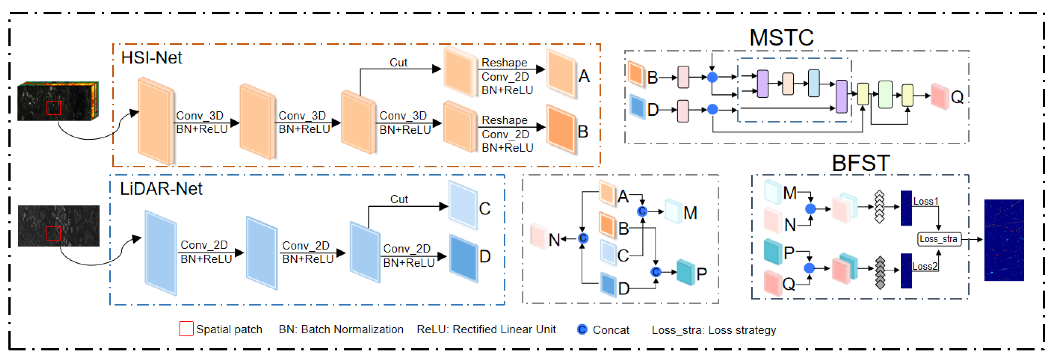
2.1. Overall Framework

To better address issues such as inconsistent data structures, irrelevant physical properties, scarce training data, insufficient utilization of information, and imperfect feature fusion method, we propose an end-to-end neural network called BTRF-Net, as shown in Figure 2.

The BTRF-Net uses HSI-Net and LiDAR-Net to extract spectral and spatial features of hyperspectral images and elevation information of LiDAR data, respectively, from different levels of the network. For the HSI-Net, PCA [26] is firstly used to reconstruct hyperspectral data in order to summarize the main detail information, compress or even discard redundant information, as shown in Equation (1). Secondly, appropriate spatial patches are chosen to obtain spatial neighborhood information around given pixels, and inputted into the HSI-Net for classification. Then, we use a 3D convolutional neural network on the hyperspectral image, using 3D convolutional kernels to simultaneously sample three dimensions to extract spectral and spatial features, and to achieve fusion of spatial and spectral information, thereby fully utilizing the advantages of hyperspectral images, and use 2D convolutional processing, as shown in Equation (2). This hybrid 3D and 2D convolutional neural network [7] can effectively extract texture information of the image and the inter-channel dependencies. For the LiDAR-Net, the spatial patch located at the same spatial position as the hyperspectral data can be directly chosed. To prevent overfitting of the network, batch normalization (BN) processing was performed simultaneously.

$$X_h=PCA\left(X_{raw}\right)$$

(1)

where $X_{raw}$ and $X_h$, respectively represent the original hyperspectral data and the hyperspectral data processed by PCA [26] for dimensionality reduction.

$$B=2DCNN\left(3DCN{N}^3\left(X_h\right)\right)$$

(2)

where $X_h$ represents the hyperspectral data processed by PCA [26] for dimensionality reduction. B is the feature map of hyperspectral data

After being processed by two sub-networks (HSI-Net and LiDAR-Net), different levels of feature representations (A, B, C, and D) for two modalities of data are firstly obtained. The specific operations are as shown in Equations (2)–(5). Secondly, three fused feature maps M, N, and P were generated by fusing the feature maps A, B, C, and D according to the fusion strategy shown in Equation (6). we input the hyperspectral and LiDAR feature maps (B and D) into the multi-source Transformer complementor (MSTC) to organically combine them by utilizing their complementarity between them, in order to better capture the correlations among multi-modal features. Then, the four fusion feature maps (M, N, P, and Q) are input into the tree structure for processing, in order to obtain multiple image features with stronger representational ability, and achieve high-precision land object classification successfully. Finally, two classifiers were constructed and processed using a weighted sum method.

$$A=2DCNN\left(Cut\left(3DCN{N}^2\left(X_h\right)\right)\right)$$

(3)

where $X_h$ represents the hyperspectral data processed by PCA [26] for dimensionality reduction. Cut represents the clipping process of the obtained feature graph to cut out the insignificant information at the edge of the feature graph. Compared to feature map B, feature map A is a shallow-level feature map of hyperspectral data. A represents the shallow-level features of hyperspectral data, while B represents the deep-level features.

$$C=Cut\left(2DCN{N}^2\left(Y_{raw}\right)\right)$$

(4)

$$D=2DCN{N}^3\left(Y_{raw}\right)$$

(5)

where $Y_{raw}$ represents the original LiDAR data. Cut represents the clipping process of the obtained feature graph to cut out the insignificant information at the edge of the feature graph. C represents the shallow-level features of LiDAR data, while D represents the deep-level features.

$$M,N,P=Concat(A,C),Concat(A,D),Concat(B,D)$$

(6)

where M, N and P, respectively represent feature fusion maps at different levels of the network.

The BTRF-Net can simultaneously and fully utilize the spectral information of hyperspectral images and the elevation information of LiDAR data and can fully explore the correlation between them so as to achieve high-precision land-cover classification. This network adopts two methods, attention mechanism and joint training, to address the issue of inconsistent data structures. Specifically, the attention mechanism enhances the feature representation of each data source by weighting its features, and then fuses them together using this mechanism. The joint training method trains multiple datasets of different modalities together, sharing model parameters and feature representation to improve the model’s generalization ability. To compensate for the impact of data scarcity on classification results, this network adopts two methods: data augmentation and joint training. Specifically, data augmentation uses diverse data processing techniques, such as cropping, to utilize the shallow information in the data, thereby reducing the risk of overfitting. It improve insufficient utilization of information by extracting feature information from different network layers. The design of binary feature search tree (BFST) enhances the robustness and anti-interference capability of this network.

2.2. Multi-Source Transformer Complementor

In order to fully utilize the complementary advantages and potential interaction between different modality data and improve data fusion methods, this paper proposes a multi-source transformer complementor (MSTC), as shown in Figure 3.

The hyperspectral and LiDAR features Ki, Qi, and Vi (i = 1 represents hyperspectral, i = 2 represents LiDAR) with added position encoding information are mapped to several lower dimensions through linear layers to obtain key vectors ki, query vectors qi, and value vectors vi (i = 1 represents hyperspectral, i = 2 represents LiDAR), as shown in Equation (7).

$$(q1,k1,v1),(q2,k2,v2)=Linear(Q1,K1,V1),Linear(Q2,K2,V2)$$

(7)

Then, multiple heads of complementary attention (MHCA) are computed separately in several dimensions and concatenated for subsequent computation, as shown in Equation (8). This is beneficial for the network to obtain different patterns of data in different attention calculations, thereby simulating the multi-channel characteristics of convolutional neural networks. The MHCA can effectively capture global features and local texture information of images, hence achieving full feature fusion.

$$Z=Attention(q1,k2,v1)=softmax\left(\frac{q1{\left(k2\right)}^T}{\sqrt{d}}\right)v1$$

(8)

Based on complementary theory support and experimental verification, we ultimately chose k2, q1, and v1 to perform the calculation of multi-head complementary attention (MHCA). We performed a dot product operation between the query vector and the transpose of the key vector to calculate the correlation between the current position’s features and the features of other positions, thereby obtaining the attention matrix. Then, the softmax function is used to normalize it and a dot product operation is performed with the value vector to make the feature of each position contain global positional feature information.

We then perform a linear mapping operation on the result, obtaining an output sequence with the same shape as Q2, and add it to the value of the input feature Q2 to form a residual connection to alleviate the degradation problem of deep neural networks, as shown in Equation (9). Next, the result is normalized to improve the network’s accelerated convergence.

$$T=Norm(Q2+Linear(Z\left)\right)$$

(9)

The multi-source Transformer complementor (MSTC) first uses a multimodal feature extractor to extract features from different modalities of remote sensing data. Then, using a multi-head complementary attention mechanism, the features of different modalities are cross-encoded to promote complementarity between them. Next, multiple complementary attention heads and feedforward neural networks are used to encode and fuse the features. Finally, the fused feature, along with three other features, is input into the BFST module for further processing.

2.3. Binary Feature Search Tree

To fully utilize the characteristic information of hyperspectral and LiDAR data, this paper organizes the fused features into a hierarchical network structure with a tree-like form. By combining knowledge of deep learning and data structures, we know that learning features requires optimization using a loss function, which is essentially a mechanism for backpropagation that can be seen as retrieving and selecting features, and it can be known that full n-ary trees have the shortest path length. For simplicity, we use a full binary tree for feature construction and name it Binary Feature Search Tree (BFST).

As shown in Figure 4, after the network extracts and fuses the image features of the two modalities, The feature maps M, N, P, and Q are obtained. These four feature maps are then concatenated and subjected to adaptive average pooling to preserve more spatial information and reduce the risk of overfitting, as shown in Equation (10).

$$O_1,O_2=Concat(M,N),Concat(P,Q)$$

(10)

This method fully utilizes the spectral information, spatial information, and elevation information of two different modal data, thereby enhancing the representation ability of multiple feature maps. By utilizing the feature correlations between different levels of images, it combines local features and global features to describe the information of target objects well. In addition, the application of a full binary tree structure effectively enhances the stability and robustness of this network.

Since the BTRF-Net adopts a multi-level structure and makes predictions at different network levels, it is necessary to weight all losses to obtain the final loss function. Each output’s classification accuracy on the training data determines its weight in the weighted sum method, as shown in Equation (11). Weighting the coefficients of different branch paths can balance the importance of the gradient flow and suppress errors during backpropagation.

$$Loss={\lambda }_1\ast Los{s}_1+{\lambda }_2\ast Los{s}_2$$

(11)

This loss function effectively updates all parameters away from the output layer, thereby improving the network’s learning ability of low-level abstract features.

3. Experiments and Results

3.1. Datasets

3.1.1. Houston Datasets

The Houston dataset [42] was collected and pixel-level registered by the Houston University Airborne Laser Mapping Center in 2012, covering the campus and surrounding urban areas of the university. The dataset consists of LiDAR images and hyperspectral images, both with the same spatial resolution of 2.5 m and image size of 349 pixels × 1905 pixels. The hyperspectral image contains 144 spectral bands with wavelengths ranging from 380 nm to 1050 nm. The dataset covers 15 different land cover categories.

3.1.2. Trento Datasets

The Trento dataset [28] was collected on an ordinary farm in the southern part of Trento, Italy. It uses AISA Eagle and Optech ALTM 3100EA sensors to acquire hyperspectral and LiDAR images, respectively. The dataset consists of LiDAR images and hyperspectral images, both of which have been pixel-level registered. Both types of remote sensing images have the same spatial resolution of 1 m and image size of 166 pixels × 600 pixels. The hyperspectral image contains 63 spectral bands with wavelengths ranging from 402.89 nm to 989.09 nm. The dataset covers six different land cover categories.

3.2. Experiment Settings

All experiments in this paper were conducted on a server equipped with Windows 10 (64-bit), an Intel(R) Core(TM) I7-9700K CPU clocked at 3.60 GHz, 32 GB of RAM, an NVIDIA GeForce RTX 2080 Ti graphics card with 11GB of memory. All networks were implemented using Python 3.8.8. For network parameter configuration, we set the learning rate to 0.0001.

In addition, choosing the appropriate number of epochs is crucial for the performance of a deep learning network. If the number of epochs is too small, the model may not fully learn the patterns in the dataset, leading to decreased performance. Conversely, if the number of epochs is too large, overfitting may occur, wasting time and resources. Therefore, it is important to select an appropriate number of epochs to ensure performance while saving time and resources. Experimental results demonstrate that the network performs best on two datasets when the number of training iterations is 100.

3.3. Evaluation Metrics

To objectively and comprehensively evaluate classification results of these models, this paper uses three evaluation metrics for quantitative analysis [39,43,44]. These three evaluation metrics are Overall Accuracy (OA), Average Accuracy (AA), and Kappa Coefficient. Overall Accuracy refers to the proportion of correctly predicted samples Nr to the total number of samples N in the entire dataset. This metric is one of the important indicators for evaluating the overall classification performance of the model, as shown in Equation (12):

$$OA=\frac{Nr}{N}$$

(12)

Average Accuracy is the average of the ratio of the number of correctly predicted samples in each category to the total number of samples in that category [45,46,47,48]. Since Overall Accuracy cannot fully evaluate the classification performance of each land cover category, it is necessary to use the Average Accuracy metric to assist in evaluation, showing the model’s classification performance on different land cover categories, as shown in Equation (13):

$$AA=\frac{1}{S}\sum _{i\in S}\frac{N{r}_i}{N_i}$$

(13)

where S represents the total number of categories, the total number of samples in the i-th category is $N_i$, and the number of accurately classified samples is $N{r}_i$.

The Kappa coefficient [43,44,45,46,47] is a metric used to measure the consistency between experimental results and true land cover categories, which can clearly determine whether there is a significant difference between the two, as shown in Equations (14) and (15).

$$p_e=\frac{{\sum }_{i\in S}{a}_i\times b_i}{N^2},p_0=OA$$

(14)

$$Kappa=\frac{p_0-p_e}{1-p_e}$$

(15)

where the total number of categories and samples are denoted by C and N, respectively. The number of real samples is $a_i$, and the number of predicted samples in the i-th category is $b_i$.

3.4. Comparative Experiments

To validate the effectiveness of the BTRF-Net, several groups of experiments are designed to compare and analyze the proposed BTRF-Net with traditional methods and several advanced deep learning networks using two datasets: Houston and Trento.

3.4.1. Comparative Experiments on the Houston Dataset

To accurately evaluate the performance of different models [30,37,39,44,45,46,47,48] on the Houston dataset, we use both quantitative analysis and qualitative analysis methods for evaluation.

In

Table 1. Comparative experiments (%) of the Houston dataset. The best metric value is highlighted in bold.

Class	SVM	ELM	CNN-PPF	C-RNN	C-CNN	TB-CNN	CNN-MRF	IP-CNN	Ours
Healthy grass	82.43	83.10	83.57	83.00	84.89	83.10	85.77	85.77	96.88
Stressed grass	82.05	83.70	98.21	79.41	87.40	81.20	86.28	87.34	88.57
Synthetic grass	99.80	100.00	98.42	99.80	99.86	100.00	99.00	100.00	100.00
Trees	92.80	91.86	97.73	90.15	93.49	92.90	92.85	94.26	94.92
Soil	98.48	98.86	96.50	99.71	100.00	99.81	100.00	98.42	98.10
Water	95.10	95.10	97.20	83.21	98.77	100.00	98.15	99.91	99.15
Residential	75.47	80.04	85.82	88.06	82.81	92.54	91.64	94.59	93.33
Commercial	46.91	68.47	56.51	88.61	78.78	94.87	80.79	91.81	94.96
Road	77.53	84.80	71.20	66.01	82.51	83.85	91.37	89.35	94.03
Highway	60.04	49.13	57.12	52.22	59.41	69.89	73.35	72.43	90.18
Railway	81.02	80.27	80.55	81.97	83.24	86.15	98.87	96.57	93.11
Parking Lot 1	85.49	79.06	62.82	69.83	92.13	92.60	89.38	95.60	95.51
Parking Lot 2	75.09	71.58	63.86	79.64	94.88	79.30	92.75	94.37	98.71
Tennis Court	100.00	99.60	100.00	100.00	99.77	100.00	100.00	99.86	100.00
Running Track	98.31	98.52	98.10	100.00	98.79	100.00	100.00	99.99	99.58
OA (%)	80.49	81.29	83.33	88.55	86.90	88.91	90.61	92.06	94.47
AA (%)	83.37	84.27	83.21	90.30	89.11	90.42	92.01	93.35	95.80
KAPPA (%)	78.98	80.45	81.88	87.56	85.89	87.96	89.87	91.42	94.00

, the experimental results of different methods for each category are presented, and the optimal classification results for each category are highlighted in bold. As shown in Table 1, the BTRF-Net outperforms other comparable classification methods in evaluation metrics such as overall accuracy (OA), average accuracy (AA), and Kappa coefficient. Specifically speaking, the values of OA, AA, and Kappa coefficient reach 94.47%, 95.80%, and 94.00%, respectively. Compared to the suboptimal network IP-CNN, these three metrics were improved by 2.41%, 2.45%, and 2.58%, respectively. The BTRF-Net achieves good classification results for those objects that are easily misclassified due to similar material or texture, such as roads and highways, parking lot 1 and parking lot 2, and residential and commercial. For example, the classification accuracy of both Parking Lot 1 and Parking Lot 2 exceeded 95%, while the classification performance of other models was not as good as BTRF-Net. BTRF-Net has the best performance in terms of classification accuracy for both roads and highways, with the highest overall classification accuracy among other models. This is because it can more fully utilize the elevation information provided by the LiDAR data at different network levels, thus more accurately distinguishing objects with similar spectral information. Generally speaking, most objects are accurately classified, with only a few objects being misclassified. Therefore, the BTRF-Net effectively mitigates the misclassification problem caused by spectral similarity.

Our proposed method outperforms other methods in terms of visualization, as depicted in Figure 5. To better visualize the classification results of different methods, the highway on the right side of the image was cropped and enlarged, as shown in Figure 6.

In Figure 6, when distinguishing highways, models such as CNN MRF, C-RNN, CNN-PPF, and C-CNN cannot correctly represent the basic contours of highways. However, TB-CNN and IP-CNN perform well in this aspect and can clearly identify the basic contours of highways. Compared with other methods, our network displays the overall situation of highways more meticulously when distinguishing highways, and the visualization effect is better than other models. This is because the multi-source Transformer complementor (MSTC) can capture potential interactions between different modal features and use the complementarity and cooperation between these features to further improve the accuracy of land classification. The BTRF-Net can effectively distinguish the most objects, and even structurally similar objects such as roads and highways, healthy and stressed grasses, can be accurately classified, proving the effectiveness of this proposed network.

3.4.2. Comparative Experiments on the Trento Dataset

To accurately evaluate the performance of different models [30,37,39,44,45,46,47,48] on the Trento dataset, we use both quantitative analysis and qualitative analysis methods for evaluation.

Table 2. Comparative experiments (%) of the Trento dataset. The best metric value is highlighted in bold.

Class	SVM	ELM	CNN-PPF	C-RNN	C-CNN	TB-CNN	CNN MRF	IP-CNN	Ours
Apple trees	88.62	92.17	90.11	98.39	93.53	98.04	99.95	99.00	95.92
Buildings	94.04	90.91	83.34	90.46	91.97	94.56	89.97	99.40	98.04
Ground	93.53	94.36	71.13	99.79	98.33	94.36	98.33	99.10	80.33
Woods	98.90	97.12	99.04	96.96	96.50	96.57	100.00	99.92	99.83
Vineyard	88.96	78.58	99.37	100.00	98.49	99.62	100.00	99.66	99.92
Roads	91.75	63.23	89.73	81.63	71.24	74.47	97.86	90.21	97.66
OA (%)	92.77	85.81	94.76	97.30	93.73	96.44	98.40	98.58	98.66
AA (%)	92.63	86.06	88.97	94.54	94.23	92.94	97.04	97.88	95.30
KAPPA (%)	95.85	81.36	93.04	96.39	93.70	95.26	97.86	98.17	98.20

presents the experimental outcomes of various approaches for each category, and the optimal classification results for each category are highlighted in bold. We can see that the BTRF-Net outperforms other comparable classification methods in evaluation metrics such as overall accuracy (OA), average accuracy (AA), and Kappa coefficient, achieving 98.66%, 95.30%, and 98.20%, respectively. The BTRF-Net performs the best in terms of overall accuracy compared to other models. This is because we fully consider the balance of classification, thus maximizing the overall classification accuracy of the network. Although the AA of the BTRF-Net was slightly lower than the suboptimal network IP-CNN, its OA and Kappa coefficient were better than those of IP-CNN. The Kappa coefficient of this network reached 98.20%, which is better than other classifiers. In general, the higher the Kappa coefficient, the higher the consistency between the model’s predicted results and the real results, indicating better performance of the model.

The Figure 7 demonstrates that our proposed method has the best visualization effect. To better visualize the classification results of different methods, the road in the upper left corner of the image was cropped and enlarged, as shown in Figure 8.

In Figure 8, it can be observed that SVM and ELM generated a lot of noise when distinguishing between categories such as vineyards, roads, and apple trees. When distinguishing the roads, CNN-PPF, C-CNN, and C-RNN produced varying degrees of misclassification, while CNN-MRF and IP-CNN performed well in this aspect, being able to clearly identify the contour of the road. Compared with other models, the BTRF-Net performs better overall in classification. This is because the BTRF-Net can fully utilize the characteristic information of hyperspectral and LiDAR data from different network layers. In addition, by using the multi-source Transformer complementor (MSTC) and the complete binary tree structure to utilize the information from hyperspectral and liDAR data, the BTRF-Net achieved outstanding collaborative classification performance. This hierarchical network can extract global and local features more robustly, thereby significantly improving the accuracy of land cover classification. However, when distinguishing between apple trees and the ground, this network is slightly inferior to existing methods because it may ignore some fine-grained information.

4. Discussion

4.1. Parameter Tuning

4.1.1. Principal Component Analysis

Hyperspectral data typically contains dozens to hundreds of spectral channels, providing rich spectral information, but also containing a large amount of redundant information and noise. To reduce data dimensionality and parameter quantity while preserving important information in hyperspectral data, the data is reconstructed using PCA. In this process, the main details are retained while compressing or even discarding redundant information and noise in order to achieve better data dimensionality reduction.

As shown in Figure 9a, as the number of principal components, denoted as n, changes, the classification results of the network also change accordingly. We select different numbers of principal components (1, 5, 10, 15, 20, 25, 30, 35, and 40) and objectively evaluate the experimental results using the overall accuracy (OA). As n increases, the amount of important information retained after data reconstruction gradually increases, which is beneficial for the gradual improvement of the network’s OA value. When n reaches 30, this network can obtain the best classification results. However, when n is too large, the accuracy curve of the model becomes flat, and performance degradation may occur. This indicates that the redundant information and noise in hyperspectral data have not been fully compressed and eliminated, which has a detrimental effect on the learning of model parameters. Therefore, a balance needs to be struck between maintaining sufficient information and ensuring model performance to obtain the best classification results.

4.1.2. Selection of Spatial Patches

The spatial dimension of the input cube is also one of the determinants of the classification performance of any spectral-spatial network. Therefore, appropriate spatial patches need to be chosen to obtain spatial neighborhood information around given pixel, which can then be input into this network for classification. As the patch size changes, the classification results of the model will also change accordingly.

To objectively evaluate the classification performance under different spatial patch sizes, we selected six different patch sizes (5, 7, 9, 11, 13, and 15) and evaluated the experimental results using the OA.

As shown in Figure 9b, as the spatial patch size increases, the spatial neighborhood information contained in each patch gradually becomes more sufficient, which is beneficial for the gradual improvement of the model’s OA value. When the patch size reaches 11, the model can obtain the best classification result. However, if the spatial patch size is too large, the spatial neighborhood information in the patch will become too complex, which will interfere with the features of the central pixel and reduce the distinguishability of the patch. Therefore, the selection of spatial patch size needs to balance the full use of neighborhood information and the maintainability of patch distinguishability to achieve the best classification effect.

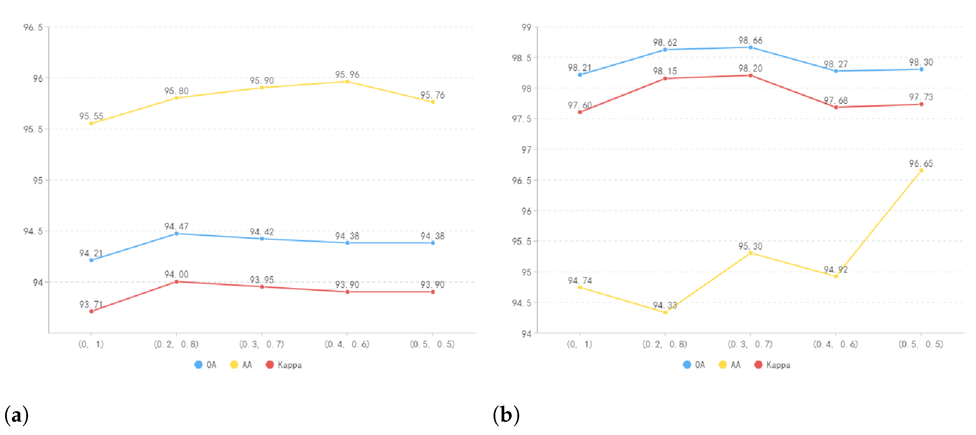
4.1.3. Graphs Comparing BFST Accuracy with Varying Weight Coefficients

The paper assigns different weighting coefficients to two distinct branches and compares their performance through experimental analysis.

According to Figure 10, it can be reasonably inferred that different weight combinations have varying impacts on several performance metrics of the network, and the differences in these impacts are highly significant and should not be overlooked. Additionally, to achieve optimal results on different datasets, the weight combinations of this network may have different requirements. It is evident that the feature extraction performance of (0, 1) is the weakest for two dataset. This is attributed to the challenges faced by a single-layer network in efficiently updating network parameters during training, thereby compromising the network’s ability to learn local information from shallow features and consequently resulting in a decline in network accuracy.

The visualization results are shown in Figure 11. To better visualize the classification results of different methods, the highway on the right side of the image was cropped and enlarged, as shown in Figure 12.

With respect to the Houston dataset, enhancing the value of ${\lambda }_1$ results in an overall improvement in the network’s performance. The optimal weight ratio of (0.2, 0.8) signifies that this weight combination yields the best balance between the requirements of primary and secondary constraints and yields the highest ovreall accuracy. Nonetheless, unrestricted weight increase leads to a continuous decline in network performance. Based on the analysis of Figure 11 and Figure 12, it is evident that the highway section is susceptible to misclassification as roads, railway, residential, among others, owing to the similarity in the composition materials. The degree of misclassification varies across different networks. Notably, the proposed network in this study exhibits superior performance compared to other networks in accurately identifying the highway. Regarding the Trento dataset, increasing the value of ${\lambda }_1$ leads to an overall improvement in network performance. The optimal weight combination with a ratio of (0.3, 0.7) means that this combination of weights achieves the best balance between satisfying the primary and secondary constraint requirements and produces the highest overall accuracy. However, an unrestricted increase in weight results in a decrease in network performance.

The proposed network can flexibly change weight combinations according to different datasets, allowing this combination of weights to achieve the best balance between satisfying the primary and secondary constraint requirements and producing the highest overall accuracy.

4.2. Ablation Experiments

4.2.1. Ablation Experiments of the Multi-Source Transformer Complementor

To verify the effectiveness of the Multi-Source Transformer Complementor, several sets of experiments were designed in this paper.

Through comparison, it can be observed that on the Houston dataset, the OA, AA, and Kappa were improved by 1.94%, 1.19%, and 2.10%, respectively for the network with the addition of MSTC as compared to the basic network (

Table 3. Ablation Experiments of the Multi-Source Transformer Complementor (%) of the Houston dataset. The best metric value is highlighted in bold.

	Basic Network	Basic Network + MSTC	BTRF-Net
OA	91.60	93.54	94.47
AA	93.67	94.86	95.80
Kappa	90.88	92.98	94.00

). In addition, compared to the baseline network, the network with the addition of MSTC on the Trento dataset resulted in an improvement of 1.22%, 3.69%, and 1.61%, in OA, AA, and Kappa, respectively (

Table 4. Ablation Experiments of the Multi-Source Transformer Complementor (%) of the Trento dataset. The best metric value is highlighted in bold.

	Basic Network	Basic Network + MSTC	BTRF-Net
OA	96.81	98.03	98.66
AA	89.68	93.37	95.30
Kappa	95.74	97.35	98.20

) [49,50,51,52,53,54]. This improvement is attributed to the utilization of complementarity and synergistic effects among multimodal feature information in remote sensing images by MSTC for better capturing their correlations. The visualization result is shown in Figure 13.

4.2.2. Ablation Experiments of the Binary Feature Search Tree

To verify the effectiveness of the Binary Feature Search Tree, several sets of experiments were designed in this paper.

By comparing the results, it is evident that the Houston dataset showed an increase of 2.05%, 1.34%, and 2.22% in OA, AA, and Kappa, respectively when using the network with BFST, as opposed to the basic network (

Table 5. Ablation Experiments of the Binary Feature Search Tree (%) of the Houston dataset. The best metric value is highlighted in bold.

	Basic Network	Basic Network + BFST	BTRF-Net
OA	91.60	93.65	94.47
AA	93.67	95.01	95.80
Kappa	90.88	93.10	94.00

). Likewise, the Trento dataset also exhibited an improvement of 1.27%, 2.83%, and 1.69% in OA, AA, and Kappa, respectively when comparing the network with BFST to the baseline network (

Table 6. Ablation Experiments of the Binary Feature Search Tree (%) of the Trento dataset. The best metric value is highlighted in bold.

	Basic Network	Basic Network + BFST	BTRF-Net
OA	96.81	98.08	98.66
AA	89.68	92.51	95.30
Kappa	95.74	97.43	98.20

) [55,56]. This is because the BFST fuses multi-modal features at different network levels to obtain multiple image features with stronger representation abilities, effectively enhancing the stability and robustness of the network. The visualization result is shown in Figure 14.

5. Conclusions

This paper proposes a deep learning network BTRF-Net which can simultaneously and fully utilize the spectral information of hyperspectral images and the elevation information of LiDAR data and can fully explore the correlation between them so as to achieve high-precision land-cover classification. Firstly, the introduction of PCA allows the network to retain the main details of hyperspectral images while compressing or even discarding redundant information and noise, thus improving the performance of the network. Secondly, the MSTC utilizes the complementarity and cooperation among multimodal feature information in remote sensing images to better capture their correlation. Then, the BFST enhances the robustness and anti-interference capability of this network. Finally, multiple sets of experiments were conducted to validate the effectiveness of our network on two datasets. The experimental results demonstrate that the proposed network outperforms other networks in terms of accuracy. This study has important practical value in civil and military fields.

References

1. Masser, I. Managing our urban future: The role of remote sensing and geographic information systems. Habit. Int. 2001, 25, 503–512. [Google Scholar] [CrossRef]
2. Maes, W.H.; Steppe, K. Estimating evapotranspiration and drought stress with ground-based thermal remote sensing in agriculture: A review. J. Exp. Bot. 2012, 63, 4671–4712. [Google Scholar] [CrossRef] [PubMed]
3. Fan, J.; Zhang, X.; Su, F.; Ge, Y.; Tarolli, P.; Yang, Z.; Zeng, C.; Zeng, Z. Geometrical feature analysis and disaster assessment of the Xinmo landslide based on remote sensing data. J. Mount. Sci. 2017, 14, 1677–1688. [Google Scholar] [CrossRef]
4. Ghosh, P.; Roy, S.K.; Koirala, B.; Rasti, B.; Scheunders, P. Deep hyperspectral unmixing using transformer network. arXiv 2022, arXiv:2203.17076. [Google Scholar]
5. Pham, H.M.; Yamaguchi, Y.; Bui, T.Q. A case study on the relation between city planning and urban growth using remote sensing and spatial metrics. Landsc. Urban Plan. 2011, 100, 223–230. [Google Scholar] [CrossRef]
6. Carfagna, E.; Gallego, F.J. Using remote sensing for agricultural statistics. Int. Stat. Rev. 2005, 73, 389–404. [Google Scholar] [CrossRef]
7. Roy, S.K.; Krishna, G.; Dubey, S.R.; Chaudhuri, B.B. HybridSN: Exploring 3-D–2-D CNN feature hierarchy for hyperspectral image classification. IEEE Geosci. Remote Sens. Lett. 2019, 17, 277–281. [Google Scholar] [CrossRef]
8. Li, W.; Du, Q. Gabor-filtering-based nearest regularized subspace for hyperspectral image classification. IEEE J. Sel. Top. Appl. Earth Observ. Remote Sens. 2014, 7, 1012–1022. [Google Scholar] [CrossRef]
9. Chen, Y.; Nasrabadi, N.M.; Tran, T.D. Hyperspectral image classification using dictionary-based sparse representation. IEEE Trans. Geosci. Remote Sens. 2011, 49, 3973–3985. [Google Scholar] [CrossRef]
10. Benediktsson, J.A.; Palmason, J.A.; Sveinsson, J.R. Classification of hyperspectral data from urban areas based on extended morphological profiles. IEEE Trans. Geosci. Remote Sens. 2005, 43, 480–491. [Google Scholar] [CrossRef]
11. Gowen, A.A.; O’Donnell, C.P.; Cullen, P.J.; Downey, G.; Frias, J.M. Hyperspectral imaging–an emerging process analytical tool for food quality and safety control. Trends Food Sci. Technol. 2007, 18, 590–598. [Google Scholar] [CrossRef]
12. Stuffler, T.; Förster, K.; Hofer, S.; Leipold, M.; Sang, B.; Kaufmann, H.; Penn, B.; Mueller, A.; Chlebek, C. Hyperspectral imaging—An advanced instrument concept for the EnMAP mission (Environmental Mapping and Analysis Programme). Acta Astronaut. 2009, 65, 1107–1112. [Google Scholar] [CrossRef]
13. Plaza, A.; Du, Q.; Chang, Y.L.; King, R.L. High performance computing for hyperspectral remote sensing. IEEE J. Sel. Top. Appl. Earth Observ. Remote Sens. 2011, 4, 528–544. [Google Scholar] [CrossRef]
14. Roy, S.K.; Deria, A.; Hong, D.; Ahmad, M.; Plaza, A.; Chanussot, J. Hyperspectral and LiDAR data classification using joint CNNs and morphological feature learning. IEEE Trans. Geosci. Remote Sens. 2022, 60, 1–16. [Google Scholar] [CrossRef]
15. Rasti, B.; Ghamisi, P.; Plaza, J.; Plaza, A. Fusion of hyperspectral and LiDAR data using sparse and low-rank component analysis. IEEE Trans. Geosci. Remote Sens. 2017, 55, 6354–6365. [Google Scholar] [CrossRef]
16. Zhang, J.; Lin, X.; Ning, X. SVM-based classification of segmented airborne LiDAR point clouds in urban areas. Remote Sens. 2013, 5, 3749–3775. [Google Scholar] [CrossRef]
17. Xu, T.; Gao, X.; Yang, Y.; Xu, L.; Xu, J.; Wang, Y. Construction of a Semantic Segmentation Network for the Overhead Catenary System Point Cloud Based on Multi-Scale Feature Fusion. Remote Sens. 2022, 14, 2768. [Google Scholar] [CrossRef]
18. Chen, Y.; Li, C.; Ghamisi, P.; Shi, C.; Gu, Y. Deep fusion of hyperspectral and LiDAR data for thematic classification. In Proceedings of the 2016 IEEE International Geoscience and Remote Sensing Symposium (IGARSS), IEEE, Beijing, China, 10–15 July 2016; pp. 3591–3594. [Google Scholar]
19. Tomljenovic, I.; Höfle, B.; Tiede, D.; Blaschke, T. Building extraction from airborne laser scanning data: An analysis of the state of the art. Remote Sens. 2015, 7, 3826. [Google Scholar] [CrossRef]
20. Zhang, M.; Ghamisi, P.; Li, W. Classification of hyperspectral and LiDAR data using extinction profiles with feature fusion. Remote Sens. Lett. 2017, 8, 957–966. [Google Scholar] [CrossRef]
21. Ghamisi, P.; Rasti, B.; Yokoya, N.; Wang, Q.; Hofle, B.; Bruzzone, L.; Bovolo, F.; Chi, M.; Anders, K.; Gloaguen, R.; et al. Multisource and multitemporal data fusion in remote sensing: A comprehensive review of the state of the art. IEEE Geosci. Remote Sens. Mag. 2019, 7, 6–39. [Google Scholar] [CrossRef]
22. Hang, R.; Li, Z.; Ghamisi, P.; Hong, D.; Xia, G.; Liu, Q. Classification of hyperspectral and LiDAR data using coupled CNNs. IEEE Trans. Geosci. Remote Sens. 2020, 58, 4939–4950. [Google Scholar] [CrossRef]
23. Debes, C.; Merentitis, A.; Heremans, R.; Hahn, J.; Frangiadakis, N.; van Kasteren, T.; Liao, W.; Bellens, R.; Piurica, A.; Gautama, S.; et al. Hyperspectral and LiDAR data fusion: Outcome of the 2013 GRSS data fusion contest. IEEE J. Sel. Top. Appl. Earth Observ. Remote Sens. 2014, 7, 2405–2418. [Google Scholar] [CrossRef]
24. Pohl, C.; Van Genderen, J.L. Review article multisensor image fusion in remote sensing: Concepts, methods and applications. Int. J. Remote Sens. 1998, 19, 823–854. [Google Scholar] [CrossRef]
25. Pedergnana, M.; Marpu, P.R.; Dalla Mura, M.; Dalla Mura, M.; Benediktsson, J.A.; Bruzzone, L. Classification of remote sensing optical and LiDAR data using extended attribute profiles. IEEE J. Sel. Top. Signal Process. 2012, 6, 856–865. [Google Scholar] [CrossRef]
26. Réjichi, S.; Chaabane, F. Feature extraction using PCA for VHR satellite image time series spatio-temporal classification. In Proceedings of the 2015 IEEE International Geoscience and Remote Sensing Symposium (IGARSS), IEEE, Milan, Italy, 26–31 July 2015; pp. 485–488. [Google Scholar]
27. Liao, W.; Pižurica, A.; Bellens, R.; Gautama, S.; Philips, W. Generalized graph-based fusion of hyperspectral and LiDAR data using morphological features. IEEE Geosci. Remote Sens. Lett. 2014, 12, 552–556. [Google Scholar] [CrossRef]
28. Rasti, B.; Ghamisi, P.; Gloaguen, R. Hyperspectral and LiDAR fusion using extinction profiles and total variation component analysis. IEEE Trans. Geosci. Remote Sens. 2017, 55, 3997–4007. [Google Scholar] [CrossRef]
29. Liao, W.; Bellens, R.; Pižurica, A.; Gautama, S.; Philips, W. Combining feature fusion and decision fusion for classification of hyperspectral and LiDAR data. In Proceedings of the 2014 IEEE Geoscience and Remote Sensing Symposium, IEEE, Quebec City, QC, Canada, 13–18 July 2014; pp. 1241–1244. [Google Scholar]
30. Hearst, M.A.; Dumais, S.T.; Osuna, E.; Platt, J.; Scholkopf, B. Support vector machines. IEEE Intell. Syst. Their Appl. 1998, 13, 18–28. [Google Scholar] [CrossRef]
31. Ge, C.; Du, Q.; Li, W.; Li, Y.; Sun, W. Hyperspectral and LiDAR data classification using kernel collaborative representation based residual fusion. IEEE J. Sel. Top. Appl. Earth Observ. Remote Sens. 2019, 12, 1963–1973. [Google Scholar] [CrossRef]
32. Zhong, Y.; Cao, Q.; Zhao, J.; Ma, A.; Zhao, B.; Zhang, L. Optimal decision fusion for urban land-use/land-cover classification based on adaptive differential evolution using hyperspectral and LiDAR data. Remote Sens. 2017, 9, 868. [Google Scholar] [CrossRef]
33. Zhu, X.X.; Tuia, D.; Mou, L.; Xia, G.S.; Zhang, L.; Xu, F.; Fraundorfer, F. Deep learning in remote sensing: A comprehensive review and list of resources. IEEE Geosci. Remote Sens. Mag. 2017, 5, 8–36. [Google Scholar] [CrossRef]
34. Xu, Y.; Du, B.; Zhang, L. Multi-source remote sensing data classification via fully convolutional networks and post-classification processing. In Proceedings of the IGARSS 2018-2018 IEEE International Geoscience and Remote Sensing Symposium, IEEE, Valencia, Spain, 22–27 July 2018; pp. 3852–3855. [Google Scholar]
35. Zhang, M.; Li, W.; Du, Q.; Gao, L.; Zhang, B. Feature extraction for classification of hyperspectral and LiDAR data using patch-to-patch CNN. IEEE Trans. Cybern. 2018, 50, 100–111. [Google Scholar] [CrossRef] [PubMed]
36. Mohla, S.; Pande, S.; Banerjee, B.; Chaudhuri, S. Fusatnet: Dual attention based spectrospatial multimodal fusion network for hyperspectral and lidar classification. In Proceedings of the IEEE/CVF Conference on Computer Vision and Pattern Recognition Workshops, Seattle, WA, USA, 13–19 June 2020; pp. 92–93. [Google Scholar]
37. Cao, X.; Zhou, F.; Xu, L.; Meng, D.; Xu, Z.; Paisley, J. Hyperspectral image classification with Markov random fields and a convolutional neural network. IEEE Trans. Image Process. 2018, 27, 2354–2367. [Google Scholar] [CrossRef] [PubMed]
38. Hong, D.; Gao, L.; Hang, R.; Zhang, B.; Chanussot, J. Deep encoder–decoder networks for classification of hyperspectral and LiDAR data. IEEE Geosci. Remote Sens. Lett. 2020, 19, 1–5. [Google Scholar] [CrossRef]
39. Wu, H.; Prasad, S. Convolutional recurrent neural networks for hyperspectral data classification. Remote Sens. 2017, 9, 298. [Google Scholar] [CrossRef]
40. Hu, R.; Singh, A. Unit: Multimodal multitask learning with a unified transformer. In Proceedings of the IEEE/CVF International Conference on Computer Vision, Montreal, BC, Canada, 11–17 October 2021; pp. 1439–1449. [Google Scholar]
41. Vaswani, A.; Shazeer, N.; Parmar, N.; Uszkoreit, J.; Jones, L.; Gomez, A.N.; Kaiser, U.; Polosukhin, I. Attention is all you need. Adv. Neural Inf. Process. Syst. 2017, 30, 5998–6008. [Google Scholar]
42. Zhang, G.; Gao, X.; Yang, Y.; Wang, M.; Ran, S. Controllably deep supervision and multi-scale feature fusion network for cloud and snow detection based on medium-and high-resolution imagery dataset. Remote Sens. 2021, 13, 4805. [Google Scholar] [CrossRef]
43. Khodadadzadeh, M.; Li, J.; Prasad, S.; Plaza, A. Fusion of hyperspectral and LiDAR remote sensing data using multiple feature learning. IEEE J. Sel. Top. Appl. Earth Observ. Remote Sens. 2015, 8, 2971–2983. [Google Scholar] [CrossRef]
44. Huang, G.B.; Zhu, Q.Y.; Siew, C.K. Extreme learning machine: Theory and applications. Neurocomputing 2006, 70, 489–501. [Google Scholar] [CrossRef]
45. Li, W.; Wu, G.; Zhang, F.; Du, Q. Hyperspectral image classification using deep pixel-pair features. IEEE Trans. Geosci. Remote Sens. 2016, 55, 844–853. [Google Scholar] [CrossRef]
46. Lee, H.; Kwon, H. Going deeper with contextual CNN for hyperspectral image classification. IEEE Trans. Image Process. 2017, 26, 4843–4855. [Google Scholar] [CrossRef]
47. Xu, X.; Li, W.; Ran, Q.; Du, Q.; Gao, L.; Zhang, B. Multisource remote sensing data classification based on convolutional neural network. IEEE Trans. Geosci. Remote Sens. 2017, 56, 937–949. [Google Scholar] [CrossRef]
48. Zhang, M.; Li, W.; Tao, R.; Li, H.; Du, Q. Information fusion for classification of hyperspectral and LiDAR data using IP-CNN. IEEE Trans. Geosci. Remote Sens. 2021, 60, 1–12. [Google Scholar] [CrossRef]
49. Ding, Y.; Zhang, Z.-L.; Zhao, X.-F.; Cai, W.; He, F.; Cai, Y.-M.; Cai, W.-W. Deep hybrid: Multi-graph neural network collaboration for hyperspectral image classification. Def. Technol. 2023, 23, 164–176. [Google Scholar]
50. Ding, Y.; Zhang, Z.; Zhao, X.; Hong, D.; Li, W.; Cai, W.; Zhan, Y. AF2GNN: Graph convolution with adaptive filters and aggregator fusion for hyperspectral image classification. Inf. Sci. 2022, 602, 201–219. [Google Scholar] [CrossRef]
51. Ding, Y.; Zhang, Z.; Zhao, X.; Cai, W.; Yang, N.; Hu, H.; Huang, X.; Cao, Y.; Cai, W. Unsupervised self-correlated learning smoothy enhanced locality preserving graph convolution embedding clustering for hyperspectral images. IEEE Trans. Geosci. Remote Sens. 2022, 60, 1–16. [Google Scholar] [CrossRef]
52. Ding, Y.; Zhao, X.; Zhang, Z.; Cai, W.; Yang, N.; Zhan, Y. Semi-supervised locality preserving dense graph neural network with ARMA filters and context-aware learning for hyperspectral image classification. IEEE Trans. Geosci. Remote Sens. 2021, 60, 1–12. [Google Scholar] [CrossRef]
53. Ding, Y.; Zhao, X.; Zhang, Z.; Cai, W.; Yang, N. Graph sample and aggregate-attention network for hyperspectral image classification. IEEE Geosci. Remote Sens. Lett. 2021, 19, 1–5. [Google Scholar] [CrossRef]
54. Fang, S.; Li, K.; Li, Z. S²ENet: Spatial–spectral cross-modal enhancement network for classification of hyperspectral and LiDAR data. IEEE Geosci. Remote Sens. Lett. 2022, 19, 1–5. [Google Scholar]
55. Wang, N.; Li, W.; Tao, R.; Du, Q. Graph-based block-level urban change detection using Sentinel-2 time series. Remote Sens. Environ. 2022, 274, 112993. [Google Scholar] [CrossRef]
56. Ran, S.; Gao, X.; Yang, Y.; Li, S.; Zhang, G.; Wang, P. Building multi-feature fusion refined network for building extraction from high-resolution remote sensing images. Remote Sens. 2021, 13, 2794. [Google Scholar] [CrossRef]
Figure 1. Spectral information of classes in the Houston dataset.
Remotesensing 15 02706 g001
Figure 2. The main structure of the network.
Remotesensing 15 02706 g002
Figure 3. Multi-Source Transformer Complementer.
Remotesensing 15 02706 g003
Figure 4. Binary Feature Search Tree.
Remotesensing 15 02706 g004
Figure 5. Visualization results of the Houston dataset.
Remotesensing 15 02706 g005
Figure 6. Visualization results of the right highway in Houston dataset.
Remotesensing 15 02706 g006
Figure 7. Visualization results of Trento dataset.
Remotesensing 15 02706 g007
Figure 8. Visualization results of the upper left side road in Trento dataset.
Remotesensing 15 02706 g008
Figure 9. The trend chart. n is the number of principal components. (a) The relationship between n and OA; (b) The relationship between Spatial patch sizes and OA.
Remotesensing 15 02706 g009
Figure 10. Graphs of various performance metrics for BFST with different weighted combinations. (a) The performance of BFST with different weights on the Houston; (b) The performance of BFST with different weights on the Trento.
Remotesensing 15 02706 g010
Figure 11. Visualization results of BTRF-Net with Varying Weight Coefficients of the BFST.
Remotesensing 15 02706 g011
Figure 12. Visualization results of BTRF-Net with Varying Weight Coefficients of the BFST of the right highway in Houston dataset.
Remotesensing 15 02706 g012
Figure 13. Visualization results of ablation experiments of the MSTC of Houston dataset.
Remotesensing 15 02706 g013
Figure 14. Visualization results of ablation experiments of the BFST of Houston dataset.
Remotesensing 15 02706 g014