Article

Determination of Susceptibility to the Generation of Discontinuities Related to Land Subsidence Using the Frequency Ratio Method in the City of Aguascalientes, Mexico

by
Hugo Luna-Villavicencio
1,
Jesús Pacheco-Martínez
2,*,
Gil H. Ochoa-González
3,
Martín Hernández-Marín
2,
Victor M. Hernández-Madrigal
4,
Rubén A. López-Doncel
5 and
Isaí G. Reyes-Cedeño
1,6
1
Doctorado en Ciencias de los Ámbitos Antrópicos, Departamento de Ingeniería Civil, Universidad Autónoma de Aguascalientes, Aguascalientes 20100, Mexico
2
Departamento de Ingeniería Civil, Universidad Autónoma de Aguascalientes, Aguascalientes 20100, Mexico
3
Departamento de Hábitat y Desarrollo Urbano, Instituto Tecnológico y de Estudios Superiores de Occidente, San Pedro Tlaquepaque 45604, Mexico
4
Instituto de Investigación de Ciencias de la Tierra, Universidad Michoacana de San Nicolás de Hidalgo, Morelia 58060, Mexico
5
Instituto de Geología, Universidad Autónoma de San Luis Potosí, San Luis Potosí 78760, Mexico
6
Facultad de Ingeniería, Universidad Panamericana, Aguascalientes 45010, Mexico
*
Author to whom correspondence should be addressed.
Remote Sens. 2023, 15(10), 2597; https://doi.org/10.3390/rs15102597
Submission received: 6 April 2023 / Revised: 9 May 2023 / Accepted: 9 May 2023 / Published: 16 May 2023

Abstract

:
Land subsidence in the Aguascalientes Valley, documented since the 1980s, has developed a large number of discontinuities that damage infrastructure. There is currently no methodology to accurately predict the site and time at which a discontinuity will occur, making it difficult to make decisions in urban planning or risk management. However, it is possible to determine the susceptibility of an area to the generation of fractures based on the factors associated with their formation. This study presents a zoning method based on the ground failure susceptibility index (GFSI) in the city of Aguascalientes, using the frequency ratio (FR) method and employing the depth of the basement, the subsidence rate, the subsidence gradient, and the groundwater level drawdown as variables. The zoning method included three categories of land subsidence susceptibility to fracturing, moderate, high, and very high, which were divided using the first (3.76) and second (4.24) quartiles of the GFSI. The zoning method was created with the discontinuities reported in 2010 and was validated with data from 2022. The results obtained show that 11.19% of the discontinuities developed between 2010 and 2022 were located in a zone of moderate susceptibility, 41.97% were located in a zone of high susceptibility, and 46.87% were located in a zone classified as having very high susceptibility.

Graphical Abstract

1. Introduction

Land subsidence is a growing concern for construction and infrastructure in countries around the world, including Thailand, Italy, China, the United States, Indonesia, India, Iran, Spain, Japan, and Mexico [1]. In Mexico, several cities, including San Luis Potosi, Queretaro, Celaya, Salamanca, Morelia, Tepic, Zamora, Puebla, Toluca, Jocotepec, Ciudad Guzmán, and Aguascalientes, have experienced this problem [2,3,4,5].
Groundwater extraction in the Aguascalientes Valley has caused fractures and active faults in an area of 900 km2 as reported in 2012 [6]. By 2022, using velocity maps derived from InSAR images, it was found that subsidence associated with groundwater extraction covered 878 km2, indicating that the affected areas had not increased. This regional subsidence can also lead to differential settlements and terrain fractures. In Aguascalientes, reports of active surface discontinuities date back to 1981 [7], suggesting that land subsidence due to the overexploitation of the aquifer began earlier than previously thought.
The nomenclature used in this work to differentiate between the two types of surface discontinuities in the terrain observed in the Aguascalientes Valley is as follows [8]. The term ‘surface fault’ is used when two blocks formed by the same substratum or by different substrata move parallel to the rupture plane. The term ‘earth fissure’ refers to discontinuities whose blocks, generated through the breaking of the substrate, floor, or rock due to tensional stressors, only present displacements perpendicular to the fracture plane. The term ‘ground failure’ can be used to refer to both of the types described above.
Various studies have proposed methods to develop susceptibility maps for land subsidence using different techniques, or land subsidence hazard maps [9], which is a problem affecting construction and infrastructure in many parts of the world [10,11,12,13,14,15,16,17,18]. However, few have tackled the problem of generating or reactivating the faults and fractures associated with subsidence. Some studies have used numerical models to investigate this problem, such as those of Ye et al. (2018), who defined the trace where a fracture can be generated due to high topography in the underlying rock floor of the deformable fills of the aquifer [8], and He et al. (2020), who reproduced the same high topography configuration of the bedrock in a scaled model to investigate under what conditions and how fractures associated with this bedrock configuration occur [19]. Zang et al. (2021) proposed a method for mapping the susceptibility to earth fissuring associated with tectonic forces and anthropogenic activities by integrating the analytical hierarchical process (AHP) method, the area under the curve (AUC), and the certainty factor model (CFM) [20]; this method identifies areas that are more likely to experience earth fissures based on factors such as land use, soil type, and topography. Risk management against land-subsidence-induced fractures is a crucial challenge. However, the current methods for determining susceptibility rely on regional geological information and observations, such as the area affected by subsidence, active faults, and geological formations.
While these factors are useful, they do not directly address the mechanisms that generate fractures. To improve fracture prediction, other factors, such as the shape of the bedrock, subsidence gradient, water table drawdown, and aquifer thickness, must be considered [6,21,22,23,24,25]. Although recent studies, such as that of Zang et al. (2021), have proposed methods to map the susceptibility to fractures, their results have not yet been validated. Therefore, future studies should evaluate the validity of these approaches by assessing the occurrence of new fractures in areas identified as having a high susceptibility to fracturing.
This paper presents a method for generating susceptibility maps for ground cracking associated with groundwater extraction. The method uses variables that have been identified in the literature as contributing to ground discontinuities and applies the frequency ratio method in the analysis and correlation. The variables used in the method are specified in the literature. To validate the susceptibility map, variable values from 2007 to 2011 and an inventory of the discontinuities reported in 2010 were used. The results indicate that the fractures generated between 2010 and 2022 are primarily located in areas with high and very high susceptibility.

Description of the Study Area

The study area is located within the Aguascalientes Valley, where the aquifer system is composed of poorly consolidated alluvial and lacustrine sedimentary materials [6]. It is a predominantly urban area within the city of Aguascalientes that covers a total area of 78.33 km2. The climatological and hydrogeological conditions of the Aguascalientes Valley are favorable for the development of discontinuities due to subsidence [26] since (a) the aquifer system is mainly composed of poorly consolidated sedimentary fillings; (b) the valley has a semi-arid climate and no surface water deposits, so the aquifer undergoes long periods of groundwater pumping; and (c) differential subsidence occurs due to lateral variations in the thickness of the fillings that form the aquifer. Figure 1 shows the study area within the context of the Aguascalientes Valley with the terrain discontinuities.
According to INEGI [27], the Aguascalientes Valley ranks second in the land subsidence rate among the areas experiencing subsidence in México and third in surface area affected by subsidence, making it one of the most studied places in Mexico for subsidence and cracking [6,7,28,29,30,31,32,33,34].
The generation of new cracks in the Aguascalientes Valley has significantly increased in the last 10 years. In 2013, 207 discontinuities with a total length of 321,159 m were recorded [6]; currently, 802 discontinuities with a total length of 361,938 m are registered [35]. Additionally, different types of discontinuities have been documented in the Aguascalientes Valley, such as faults due to tertiary tectonism that are currently inactive, faults generated by differential land subsidence, faults reactivated by land subsidence, and fractures reactivated by paleochannels [6,29]. For the development of the fracture susceptibility map presented in this study, we only considered discontinuities generated by differential land subsidence and reactive faults due to land subsidence. Other types of discontinuities, such as faults due to tertiary tectonism and fractures reactivated by paleochannels, were not included.
Initially, fault and fracture mapping was only carried out for the city of Aguascalientes [36,37,38]. Currently, mapping covers the entire Aguascalientes Valley and is publicly available online [35]. For the susceptibility analysis presented in this paper, we considered the fault and fracture mapping reported in SOPMA [38] up to 2010, and we used the updated mapping presented in SIFAGG 2022 [35] to validate our results.

2. Materials and Methods
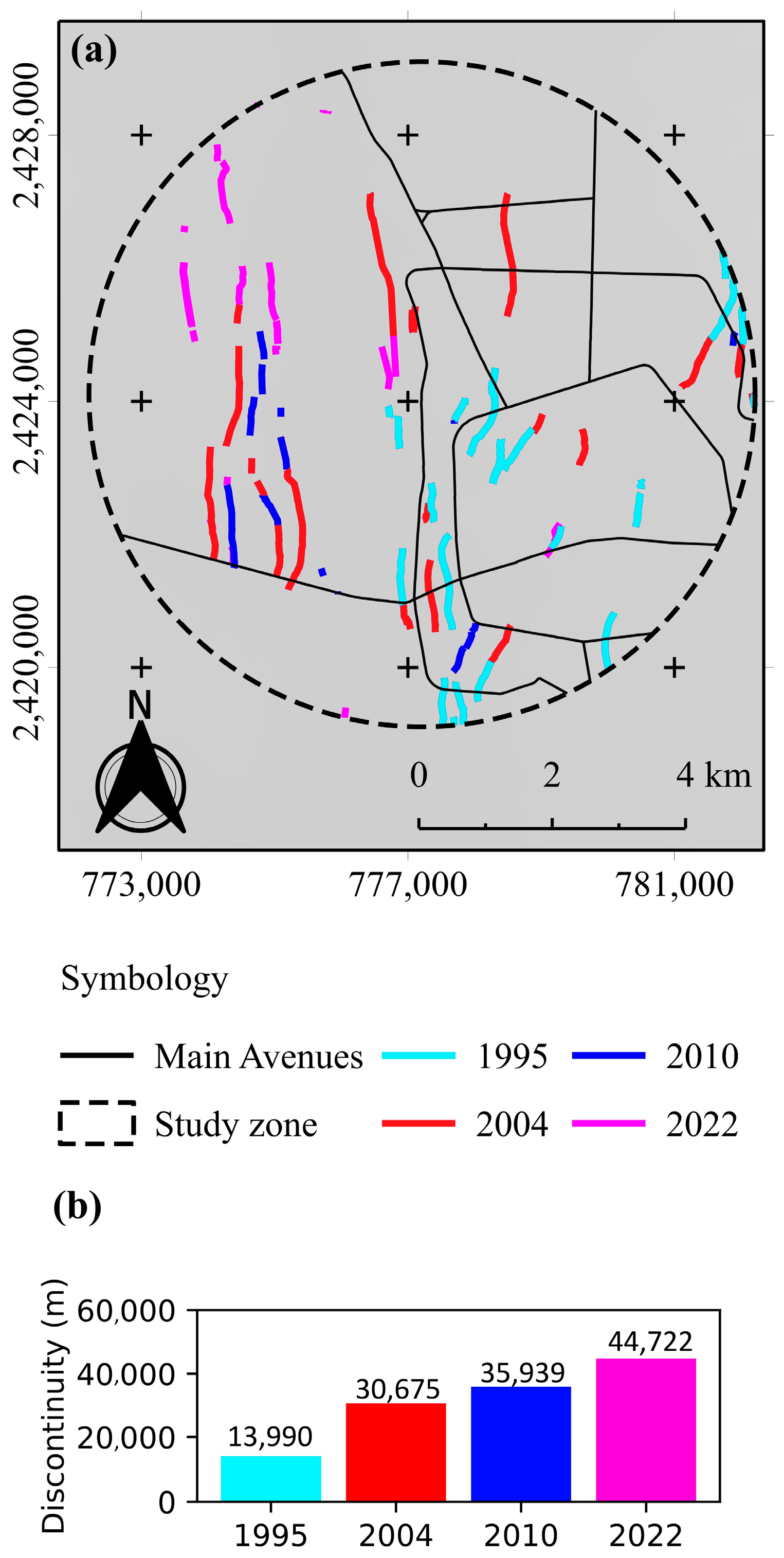
To evaluate the susceptibility of generating new faults and fractures in the study area (Figure 1b), we applied the frequency ratio (FR) method, a statistical technique that uses geographic information. To implement this technique, it is convenient to use geographic information systems. The FR method involves quantifying the magnitude and frequency of the variables associated with the occurrence of the studied phenomenon. The variables are worked in layers in raster images, where each pixel contains information about its spatial location (longitude and latitude) and the value of the variable at that location. We determined the number of classes into which each variable was divided by testing different numbers of classes and attempting to find a trend between the classes and RF. For this study, we divided the variables into three to four classes.
In this study, we used the FR technique to develop an index that identified the combination of variables and their magnitudes that were present in fault and fracture zones. A high FR value indicated the presence of faults and fractures, resulting in a high index value. There were also zones that did not exhibit discontinuities but had a high index value because they fell within classes with high frequency ratios. This suggested that the variables associated with the generation of faults existed but that the faults themselves had not yet developed. These zones were therefore considered prone to cracking.
The data correlation analysis was carried out using the free software Qgis (version 3.18.2). The final result was a susceptibility index which, in this work, was called ground failure susceptibility index (GFSI), which was determined by applying Equations (1) and (2) of the FR technique [39].
The variables used in this study, which, according to the literature, are involved in the process of generating cracking, were (a) the depth of the rock layer underlying the consolidating sediments, (b) the subsidence accumulated during the analysis period, (c) the horizontal subsidence gradient, and (d) the lowering of the water table. Changes in lithology, which is also an important variable for the formation of discontinuities, were not considered in this research, as there was only one type of material within the study area.
The variables used were based on data from 2007 and 2011 and were chosen due to the availability of information on subsidence and water table lowering. This analysis period was selected to produce a susceptibility map that could be verified against records of new fractures developed from 2010 to the present.
F r i = N p i x / N p t   N p i x /   N p t
where Fri is the frequency ratio for the i-th variable, Npix is the number of pixels in the class, ∑Npix is the total number of pixels of a variable in the entire study area, Npt is the number of points defining the trace of fractures in the class, and ∑Npt is the total number of points defining the trace of all fractures in the study area.
To obtain the GFSI, it was first necessary to divide the studied variable into classes; to obtain Npix and ∑Npix; then, to obtain Npt and ∑Npt. Next, Equation (1) was used to obtain the frequency ratio for the variable under study. This procedure was repeated for each of the variables studied.
The FR for each class was calculated, and this value was assigned to all pixels within that class for each of the four variables. The resulting maps for each variable were then used to calculate the GFSI by adding the frequency ratio value for each variable of each pixel as shown in Equation (2). Figure 2 provides a schematic representation of this procedure.
G F S I = F r I + F r 2 + F r 3 + F r 4
The variables used to determine the GFSI (Figure 3) are listed below, and how they were obtained is explained.
(a)
Bedrock depth. The thickness of the fill materials in the Aguascalientes Valley, which have consolidation potential, was obtained through gravimetric surveys [40]. The values of the depth of bedrock were categorized into 3 classes as shown in Figure 3a.
(b)
The LOS deformation accumulated during the analysis period was calculated from the results of previous investigation [40] in which a subsidence velocity map of the Aguascalientes Valley based on 34 ALOS satellite INSAR images was developed using the SBAS technique. The subsidence values were categorized into 4 classes as shown in Figure 3b. Although the variable associated with the generation of fractures is the vertical deformation, for this work, the LOS deformation was used, which was proportional to the real vertical subsidence.
(c)
Zones with differential subsidence were determined based on the subsidence gradient according to [41,42]. The values of differential subsidence were categorized into 3 classes as shown in Figure 3c.
(d)
The water table drawdown was calculated from the difference between the water table level in 2011 and that in 2007; the data was obtained from the official CONAGUA website [43]. The magnitude of the drawdown was classified into 3 classes as shown in Figure 3d. In total, 101 wells within the Aguascalientes Valley were used, the location of which is shown in Figure 4.
The original technique requires the information of the studied phenomenon to be expressed in points. However, the traces of the terrain discontinuities are linear entities; therefore, in this study, they were discretized into points spaced two meters apart to achieve adequate resolution of the discontinuities without duplicating information.
Since the range of values for each variable was different, the number of classes into which they were divided was also different. The images of the variables over the study area were discretized into pixels with a resolution of 30 by 30 m, which is the resolution of the digital elevation model used.
To eliminate errors associated with class size, we identified outliers for each variable. To do so, we determined the first quartiles (Q1), second quartiles (Q2), and third quartiles (Q3) as well as the interquartile range (IQR = Q3 − Q1). We calculated the lower limit with Q1 − 1.5 × IQR and the upper limit with Q3 + 1.5 × IQR. Values that fell outside these limits were considered outliers and were reclassified as extreme values in their respective class. This approach allowed us to create classes between the lower and upper limits for each variable. The data distributions, lower and upper limits, and outliers are shown in Figure 5.
The GFSI map was calculated using variables from 2007 to 2011 and discontinuities reported in 2010. In order to validate the results, this map was evaluated with discontinuities reported in 2022. Figure 6a shows the reported discontinuities in the city of Aguascalientes over different years, and Figure 6b shows the accumulated length of reported discontinuities in the Aguascalientes Valley.
The susceptibility to cracking was classified into three levels: moderate, high, and very high. Typically, studies on hazard zoning use five categories; however, this research only used three levels because the entire study area was located on sediments with high consolidation potential, making the area susceptible to cracking. The zoning method for susceptibility to cracking in this research coincided with the zoning method for subsidence hazards proposed by Pacheco-Martínez et al. in 2015 [40]. This occurred because the study area fell within the moderate and high zones proposed by Pacheco-Martínez. In addition, their study explains that areas with zero hazards are only found in locations where there are no materials with consolidation potential.
The zoning of susceptibility zones was performed based on quartiles of the GFSI value range. The moderate-susceptibility zone corresponded to pixels with GFSI ≤ Q1; the high-susceptibility zone was defined by pixels with Q1 < GFSI ≤ Q2; and finally, the very-high-susceptibility zone was defined by GFSI > Q2.

3. Results

Table 1 shows the limit values that define each class for each of the four variables with the corresponding percentages that define the frequency relationship between the fractures and the classes of each variable. The highest correlation was reported for the range of higher subsidence gradient values, with a frequency relationship value of 1.38, and the lowest correlation corresponded with the class with the highest accumulated deformation, with a frequency relationship of 0.05. Figure 7 shows the frequency relationship graphs for each class per variable studied from which the following observations can be made:
(a)
According to the graph in Figure 7a, the sediment thickness variable showed a behavior that was inversely proportional to the frequency ratio, meaning that zones with a lower thickness of fillings had a higher frequency ratio, i.e., they are areas where a greater number of discontinuities have occurred. This is consistent with the conceptual models of fracture generation reported by [6,21,22,24]. These models show that the generation of discontinuities takes place in zones where the underlying bedrock of the aquifer is shallower. This occurs where there is a lateral change in the depth of the aquifer.
(b)
The graph of the accumulated deformation versus the frequency ratio (Figure 7b) suggests that the zone where the highest number of fractures has occurred was not where the deformation was the highest or the lowest; instead, the highest number of fractures occurred in the zone that corresponded to the intermediate values of accumulated deformation. According to the subsidence conceptual models [6,21,22,24], a greater sediment thickness produces greater deformation, and a smaller sediment thickness produces less deformation. Therefore, the highest number of fractures should occur in the zone of transition from the thinner to the thicker sediment layers, i.e., in the subsidence zone with intermediate values as shown in the graph of Figure 7b.
(c)
The graph in Figure 7c, which shows the frequency relationship between the subsidence gradient and the occurrence of fractures, presents a directly proportional relationship. This means that the highest number of fractures was observed in areas with a higher horizontal subsidence gradient, which is consistent with a study carried out in México City [35] in which the authors used the horizontal subsidence gradient as a parameter to identify the fracturing zones.
(d)
The graph in Figure 7d suggests an inversely proportional relationship between the generation of fractures and the lowering of the water table. Figure 7d shows that the highest number of fractures occurred outside the cone of depression, which is consistent with [44,45]. They noted that the greatest subsidence occurs in areas where the lowering of the water table is highest; that fractures occur at the edges of the subsidence zone; and that, therefore, they occur outside the cone of depression, where the water level drop is lower.

4. Discussion

Figure 8 shows a map of the GFSI that defines the level of susceptibility to the generation of fracturing based on the frequency relationship of the four analyzed variables with the presence of cracking. The resulting GFSI values ranged from 2.6 to 5.12, with higher values representing areas with greater susceptibility to cracking.
Figure 9 shows a histogram of the distribution of values obtained from the GFSI, which presented a range from 1.78 to 5.12. The histogram has a negative or left skewness, which means that the majority of the study area was in a zone of very high susceptibility; meanwhile, some areas had medium values, and there were some outliers up to 2.60. The zoning was done as follows: from 0 to 3.76 (Q1), it was considered to be moderately susceptible; from Q1 to Q2 (4.24), it was considered to be high-risk zoning; and values higher than Q2 were considered to represent very high susceptibility. Within the range of GFSI values, there were values below the lower limit that were calculated with Q1 − 1.5 × (Q3 − Q1), which were considered to be outliers. These values represent the pixels with the least susceptibility to cracking, but, being outliers, they were considered to be within the moderate-susceptibility zone.
The zoning method for susceptibility to cracking, developed with the information on cracking that is available up to the year 2010, is presented in Figure 10a. Figure 10b shows the same susceptibility zoning with the updated discontinuities up to the year 2022. The moderate-susceptibility zone represents 22.62% of the total area; meanwhile, the high-susceptibility zone represents 25.87% of the total area, and the very-high-susceptibility zone represents 51.51% of the total area.
After zoning, the percentage of total discontinuities was counted in each zone, first for the year 2010 in order to have a reference and to compare it with the percentage of cracks in each zone in the year 2022. In addition, the percentage of new cracks generated from 2010 to 2022 was counted for each susceptibility zone (Figure 11). In the year 2010, the percentage of total discontinuities in the moderately susceptible zone was 17.76%; in the high-susceptibility zone, it was 34.74%; and, in the very-high-susceptibility zone, it was 47.50% (Figure 11a). For the year 2022, the percentage of total discontinuities in the moderately susceptible zone was 16.47%, that of the high-susceptibility zone was 36.16%, and that of the very-high-susceptibility zone was 47.37% (Figure 11b). Figure 11c shows that, of the new discontinuities generated from 2010 to 2022, 11.19% were generated in the moderately susceptible zone, 41.97% occurred in the high-susceptibility zone, and 48.87% were generated in the very-high-susceptibility zone.
Figure 10 shows the zoning of susceptibility to cracking, which indicates areas with a higher or lower likelihood of new discontinuities occurring based on the analysis of factors related to their genesis. Unlike the previous work [34], which presented the zoning of hazards to the effects of subsidence and cracking for the year it was conducted, this study warns about the possibility of new cracking occurrences in the future.
Some of the discontinuities used in zoning or validation may not be a result of differential subsidence caused by groundwater lowering or lateral variations in the depth of bedrock as previously explained [6,21,22,24]. Other fractures could be associated with the reactivation of paleochannels [6]. This could introduce errors in susceptibility determination. To improve the reliability of the susceptibility map, it is necessary to identify which fractures are due to this mechanism and to exclude them from the calculation.
Figure 6b shows a decrease in the generation of new cracks since 1995. In that year, the study area had 13,990 linear meters of active fractures. By 2004, the number had increased by 119.26% to 30,675 linear meters of discontinuities, with an annualized rate of new fractures of 13.25%. In 2010, the inventory of discontinuities was 35,940 m, which represents an increase of 17.16% in six years, with an annualized rate of 2.86%. By 2022, the number of faults and fractures reported was 44,722 m, an increase of 24.44% in 12 years, with an annualized rate of 2.04%. All percentages were calculated with respect to the previous record.

5. Conclusions

The application of the frequency ratio method in the development of a susceptibility map for groundwater-extraction-induced fracturing in a zone of the city of Aguascalientes as presented in this work shows that the method can be directly applied and supported through geospatial information on the factors recognized in the scientific literature as involved in the genesis of fracturing. The results of the frequency ratio found between each variable and the occurrence of fracturing are consistent with the conceptual models reported in the literature. In particular, fracturing is generated in the shallowest zones of the aquifer, where there is a lateral change in the depth of the rocky bed underlying the fill with consolidation potential, in zones where the highest values of the horizontal subsidence gradient are present and in zones outside the cone of depression.
The susceptibility zoning method that was carried out was categorized into three levels, moderate, high, and very high; the frequency ratio technique was applied to the variables and the fractures that were recorded up to 2010. The qualitative validation of this zoning method was carried out by contrasting the fractures generated from 2010 to 2022 with the obtained zones, finding that 11.19% of the discontinuities developed in areas of moderate susceptibility, 41.97% developed in areas of high susceptibility, and 46.87% developed in areas of very high susceptibility, validating the zoning method.
It is important to consider that the study area was limited to a circle with a radius of 5 km within the urban area of Aguascalientes due to the availability of information on the variables. To produce a susceptibility map that covers the peripheral non-urbanized areas outside the city, where new buildings and urban infrastructure will be constructed, more work will be required to obtain information on the entire subsidence zone.
The influence of the scale and resolution of the variable maps on the resulting susceptibility map should also be considered. More work is required to define the optimal scale and resolution of the variable maps to produce a more accurate susceptibility map that successfully defines the areas where new fractures will occur in the future. In conclusion, this work will be an important reference for the management and mitigation of the hazards associated with the presence of discontinuities in subsidence zones, and it will be a useful tool for urban development decision makers in designing less vulnerable infrastructure and in reducing the risk of fractures associated with subsidence.

Author Contributions

Conceptualization, H.L.-V.; formal analysis, H.L.-V.; investigation, H.L.-V.; methodology, J.P.-M.; project administration, J.P.-M.; supervision, J.P.-M., G.H.O.-G., M.H.-M., V.M.H.-M. and R.A.L.-D.; validation, H.L.-V.; visualization, H.L.-V. and I.G.R.-C.; writing—original draft, H.L.-V.; writing—review and editing, J.P.-M., G.H.O.-G., M.H.-M., V.M.H.-M. and R.A.L.-D. All authors have read and agreed to the published version of the manuscript.

Funding

Hugo Luna-Villavicencio (CVU Number 779284) and Isaí G. Reyes-Cedeño (CVU Number 779284) thank CONACyT for the support provided in this research.

Data Availability Statement

Data can be requested by emailing the corresponding author.

Conflicts of Interest

The authors declare no conflict of interest.

References

  1. Galloway, D.L.; Burbey, T.J. Review: Regional Land Subsidence Accompanying Groundwater Extraction. Hydrogeol. J. 2011, 19, 1459–1486. [Google Scholar] [CrossRef]
  2. Chaussard, E.; Wdowinski, S.; Cabral-Cano, E.; Amelung, F. Land Subsidence in Central Mexico Detected by ALOS InSAR Time-Series. Remote Sens. Environ. 2014, 140, 94–106. [Google Scholar] [CrossRef]
  3. Figueroa-Miranda, S.; Tuxpan-Vargas, J.; Ramos-Leal, J.A.; Hernández-Madrigal, V.M.; Villaseñor-Reyes, C.I. Land Subsidence by Groundwater Over-Exploitation from Aquifers in Tectonic Valleys of Central Mexico: A Review. Eng. Geol. 2018, 246, 91–106. [Google Scholar] [CrossRef]
  4. Cigna, F.; Tapete, D. Land Subsidence and Aquifer-System Storage Loss in Central Mexico: A Quasi-Continental Investigation with Sentinel-1 InSAR. Geophys. Res. Lett. 2022, 49, e2022GL098923. [Google Scholar] [CrossRef]
  5. Villaseñor-Reyes, C.I.; Hernández-Madrigal, V.M.; Figueroa-Miranda, S. Identification and Assessment of Land Subsidence Development in Rural Areas Using PS Interferometry: A Case Study in Western Michoacan, Mexico. Environ. Earth Sci. 2022, 81, 417. [Google Scholar] [CrossRef]
  6. Pacheco-Martínez, J.; Hernandez-Marín, M.; Burbey, T.J.; González-Cervantes, N.; Ortíz-Lozano, J.Á.; Zermeño-de-León, M.E.; Solís-Pinto, A. Land Subsidence and Ground Failure Associated to Groundwater Exploitation in the Aguascalientes Valley, México. Eng. Geol. 2013, 164, 172–186. [Google Scholar] [CrossRef]
  7. Aranda-Gómez, J.J. Geología preliminar del Graben de Aguascalientes. Rev. Mex. Cienc. Geol. 1989, 8, 22–31. [Google Scholar]
  8. Holzer, T.L. Ground Failure Induced by Graund-Water Withdrawal from Unconsolidated Sediment. Rev. Eng. Geol. 1984, 6, 67–104. [Google Scholar] [CrossRef]
  9. Fatolahzadeh, S.; Nadi, B.; Ajalloeian, R. Land Subsidence Susceptibility Zonation of Isfahan Plain Based on Geological Bedrock Layer. Geotech. Geol. Eng. 2022, 40, 1989–1996. [Google Scholar] [CrossRef]
  10. Rezaei, M.; Yazdani Noori, Z.; Dashti Barmaki, M. Land Subsidence Susceptibility Mapping Using Analytical Hierarchy Process (AHP) and Certain Factor (CF) Models at Neyshabur Plain, Iran. Geocarto Int. 2022, 37, 1465–1481. [Google Scholar] [CrossRef]
  11. Chitsazan, M.; Rahmani, G.; Ghafoury, H. Land Subsidence Susceptibility Mapping Using PWRSTFAL Framework and Analytic Hierarchy Process: Fuzzy Method (Case Study: Damaneh-Daran Plain in the West of Isfahan Province, Iran). Environ. Monit. Assess. 2022, 194, 192. [Google Scholar] [CrossRef] [PubMed]
  12. Oh, H.-J.; Syifa, M.; Lee, C.-W.; Lee, S. Land Subsidence Susceptibility Mapping Using Bayesian, Functional, and Meta-Ensemble Machine Learning Models. Appl. Sci. 2019, 9, 1248. [Google Scholar] [CrossRef]
  13. Tien Bui, D.; Shahabi, H.; Shirzadi, A.; Chapi, K.; Pradhan, B.; Chen, W.; Khosravi, K.; Panahi, M.; Bin Ahmad, B.; Saro, L. Land Subsidence Susceptibility Mapping in South Korea Using Machine Learning Algorithms. Sensors 2018, 18, 2464. [Google Scholar] [CrossRef] [PubMed]
  14. Ranjgar, B.; Razavi-Termeh, S.V.; Foroughnia, F.; Sadeghi-Niaraki, A.; Perissin, D. Land Subsidence Susceptibility Mapping Using Persistent Scatterer SAR Interferometry Technique and Optimized Hybrid Machine Learning Algorithms. Remote Sens. 2021, 13, 1326. [Google Scholar] [CrossRef]
  15. Hakim, W.L.; Achmad, A.R.; Lee, C.-W. Land Subsidence Susceptibility Mapping in Jakarta Using Functional and Meta-Ensemble Machine Learning Algorithm Based on Time-Series InSAR Data. Remote Sens. 2020, 12, 3627. [Google Scholar] [CrossRef]
  16. Pradhan, B.; Abokharima, M.H.; Jebur, M.N.; Tehrany, M.S. Land Subsidence Susceptibility Mapping at Kinta Valley (Malaysia) Using the Evidential Belief Function Model in GIS. Nat. Hazards 2014, 73, 1019–1042. [Google Scholar] [CrossRef]
  17. Zhang, B.; Zhang, L.; Yang, H.; Zhang, Z.; Tao, J. Subsidence Prediction and Susceptibility Zonation for Collapse above Goaf with Thick Alluvial Cover: A Case Study of the Yongcheng Coalfield, Henan Province, China. Bull. Eng. Geol. Environ. 2015, 75, 1117–1132. [Google Scholar] [CrossRef]
  18. Wang, H.-M.; Wang, Y.; Jiao, X.; Qian, G.-R. Risk Management of Land Subsidence in Shanghai. Desalination Water Treat. 2014, 52, 1122–1129. [Google Scholar] [CrossRef]
  19. Ye, S.; Franceschini, A.; Zhang, Y.; Janna, C.; Gong, X.; Yu, J.; Teatini, P. A Novel Approach to Model Earth Fissure Caused by Extensive Aquifer Exploitation and Its Application to the Wuxi Case, China. Water Resour. Res. 2018, 54, 2249–2269. [Google Scholar] [CrossRef]
  20. He, G.; Yan, X.; Zhang, Y.; Yang, T.; Wu, J.; Bai, Y.; Gu, D. Experimental Study on the Vertical Deformation of Soils Due to Groundwater Withdrawal. Int. J. Geomech. 2020, 20, 04020076. [Google Scholar] [CrossRef]
  21. Zang, M.; Peng, J.; Xu, N.; Jia, Z. A Probabilistic Method for Mapping Earth Fissure Hazards. Sci. Rep. 2021, 11, 8841. [Google Scholar] [CrossRef] [PubMed]
  22. Jachens, R.C.; Holzer, T.L. Geophysical Investigations of Ground Failure Related to Ground-Water Withdrawal Pichacho Basin, Arixona. Groundwater 1979, 17, 574–585. [Google Scholar] [CrossRef]
  23. Holzer, T.L.; Stanley, D.N.; Lofgren, B.E. Faulting Caused by Groundwater Extraction in Southcentral Arizona. J. Geophys. Res. Solid Earth 1979, 84, 603–612. [Google Scholar] [CrossRef]
  24. Larson, M.K. Potential for subsidence fissuring in the Phoenix Arizona USA area. Int. J. Rock Mech. Min. Sci. Geomech. Abstr. 1987, 24, 291–299. [Google Scholar] [CrossRef]
  25. Larson, M.K.; Pewe, T.L. Origin of Land Subsidence and Earth Fissuring, Northeast Phoenix, Arizona. Environ. Eng. Geosci. 1986, xxiii, 139–165. [Google Scholar] [CrossRef]
  26. Sheng, Z. Mechanisms of Earth Fissuring Caused by Groundwater Withdrawal. Environ. Eng. Geosci. 2003, 9, 351–362. [Google Scholar] [CrossRef]
  27. Burbey, T.J. The Influence of Geologic Structures on Deformation Due to Ground Water Withdrawal. Ground Water 2008, 46, 202–211. [Google Scholar] [CrossRef]
  28. INEGI. Detección de Zonas de Subsidencia En México Con Técnicas Satelitates; INEGI: Aguascalientes, México, 2022; Volume 3. [Google Scholar]
  29. Lermo-Samaniego, J.; Nieto-Obregón, J.; Zermeño, M. Fault and Fractures in the Valley of Aguascalientes. Preliminary Microzonification. In Proceedings of the 11th World Conference on Earthquake Engineering, Acapulco, Mexico, 23–28 June 1996; Elsevier: Amsterdam, The Netherlands, 1996; Volume 1651. [Google Scholar]
  30. Hernandezmarin, M.; Gonzalezcervantes, N.; Pachecomartinez, J.; Frías-Guzmán, D.H. Discussion on the Origin of Surface Failures in the Valley of Aguascalientes, México. Proc. Int. Assoc. Hydrol. Sci. 2015, 372, 235–238. [Google Scholar] [CrossRef]
  31. INEGI. Estudio de los Hundimientos por Subsidencia en Aguascalientes con Métodos Satelitales; Reporte Técnico; INEGI: Aguascalientes, México, 2016. [Google Scholar]
  32. Cigna, F.; Tapete, D. Sentinel-1 Big Data Processing with P-SBAS InSAR in the Geohazards Exploitation Platform: An Experiment on Coastal Land Subsidence and Landslides in Italy. Remote Sens. 2021, 13, 885. [Google Scholar] [CrossRef]
  33. Hernández-Marín, M.; Pacheco-Martínez, J.; Burbey, T.J.; Carreón-Freyre, D.C.; Ochoa-González, G.H.; Campos-Moreno, G.E.; de Lira-Gómez, P. Evaluation of Subsurface Infiltration and Displacement in a Subsidence-Reactivated Normal Fault in the Aguascalientes Valley, Mexico. Environ. Earth Sci. 2017, 76, 812. [Google Scholar] [CrossRef]
  34. Hernández-Marín, M.; Guerrero-Martínez, L.; Zermeño-Villalobos, A.; Rodríguez-González, L.; Burbey, T.J.; Pacheco-Martínez, J.; Martínez-Martínez, S.I.; González-Cervantes, N. Spatial and Temporal Variation of Natural Recharge in the Semi-Arid Valley of Aguascalientes, Mexico. Hydrogeol. J. 2018, 26, 2811–2826. [Google Scholar] [CrossRef]
  35. Guerrero-Martínez, L.; Hernández-Marín, M.; Burbey, T.J. Estimation of Natural Groundwater Recharge in the Aguascalientes Semiarid Valley, Mexico. Rev. Mex. Cienc. Geol. 2018, 35, 268–276. [Google Scholar] [CrossRef]
  36. Secratariat of Public Works of Aguascalientes State SIFAGG-Information System of Geological Faults and Cracks. Available online: https://www.google.com/maps/d/viewer?mid=1XSh-qhhWHKsMsdJUhAa9My8xDwA&hl=es (accessed on 25 May 2022).
  37. SOPMA-Secretariat of Public Works of the Municipality of Aguascalientes. Map of Geological Faults of Aguascalientes (in Spanish, Unpublished Map) 1995; SOPMA-Secretariat of Public Works of the Municipality of Aguascalientes: Aguascalientes, Mexico, 1995. [Google Scholar]
  38. SOPMA-Secretariat of Public Works of the Municipality of Aguascalientes. Digital System of Geological Faults of Aguascalientes (in Spanish, Unpublished Map) 2004; SOPMA-Secretariat of Public Works of the Municipality of Aguascalientes: Aguascalientes, Mexico, 2004. [Google Scholar]
  39. SOPMA-Secretariat of Public Works of the Municipality of Aguascalientes. Digital System of Geological Faults of Aguascalientes (in Spanish, Unpublished Map) 2010; SOPMA-Secretariat of Public Works of the Municipality of Aguascalientes: Aguascalientes, Mexico, 2010. [Google Scholar]
  40. Mondal, S.; Maiti, R. Integrating the Analytical Hierarchy Process (AHP) and the Frequency Ratio (FR) Model in Landslide Susceptibility Mapping of Shiv-Khola Watershed, Darjeeling Himalaya. Int. J. Disaster Risk Sci. 2013, 4, 200–212. [Google Scholar] [CrossRef]
  41. Pacheco-Martínez, J.; Cabral-Cano, E.; Wdowinski, S.; Hernández-Marín, M.; Ortiz-Lozano, J.; Zermeño-De-León, M.E. Application of InSAR and Gravimetry for Land Subsidence Hazard Zoning in Aguascalientes, Mexico. Remote Sens. 2015, 7, 17035–17050. [Google Scholar] [CrossRef]
  42. Cabral-Cano, E.; Dixon, T.H.; Miralles-Wilhelm, F.; Díaz-Molina, O.; Sánchez-Zamora, O.; Carande, R.E. Space Geodetic Imaging of Rapid Ground Subsidence in Mexico City. GSA Bull. 2008, 120, 1556–1566. [Google Scholar] [CrossRef]
  43. Barra, A.; Reyes-Carmona, C.; Herrera, G.; Galve, J.P.; Solari, L.; Mateos, R.M.; Azañón, J.M.; Béjar-Pizarro, M.; López-Vinielles, J.; Palamà, R.; et al. From Satellite Interferometry Displacements to Potential Damage Maps: A Tool for Risk Reduction and Urban Planning. Remote Sens. Environ. 2022, 282, 113294. [Google Scholar] [CrossRef]
  44. Conagua Conagua/Redes De Pozos De Monitoreo Piezométrico. Available online: https://sigagis.conagua.gob.mx/rp20/ (accessed on 25 May 2022).
  45. Amelung, F.; Galloway, D.L.; Bell, J.W.; Zebker, H.A.; Laczniak, R.J. Sensing the Ups and Downs of Las Vegas: InSAR Reveals Structural Control of Land Subsidence and Aquifer-System Deformation. Geology 1999, 27, 483. [Google Scholar] [CrossRef]
Figure 1. Study area. The dashed black line of the circle delimits the study area, the blue line represents the limits of the Aguascalientes Valley, and the red lines represent the discontinuities reported in 2022. PH represents Pabellón de Hidalgo, RR represents Rincón de Romos, SFR represents San Francisco de los Romos, T represents Tepezalá, and JGP represents Jesús Gómez Portugal. ITESM represents Instituto Tecnológico de Estudios Superiores de Monterrey, UC represents Universidad Cuauhtémoc, UAA: Universidad Autónoma de Aguascalientes, ITA: Instituto Tecnológico de Aguascalientes, and UVM represents Universidad del Valle de Mexico.
Remotesensing 15 02597 g001
Figure 2. Flowchart of the frequency ratio method.
Remotesensing 15 02597 g002
Figure 3. Variables and their classes: (a) bedrock depth, (b) subsidence velocity, (c) differential subsidence, and (d) groundwater level drawdown.
Remotesensing 15 02597 g003
Figure 4. Location of wells. Each black point represents the location of a well, the blue line represents the Valley of Aguascalientes, the black lined circle is the study zone, and the red lines are the normal faults.
Remotesensing 15 02597 g004
Figure 5. Histogram, box plot, and whisker plot for each variable. The red asterisks represent outliers for each of the variables. (a) bedrock depth, (b) subsidence velocity, (c) differential subsidence, and (d) groundwater level drawdown.
Remotesensing 15 02597 g005
Figure 6. Faults in the study area. (a) The cyan lines represent the mapped discontinuities in 1995, the red lines represent the mapped discontinuities in 2004, the blue lines represent the mapped discontinuities in 2010, and the magenta lines represent the discontinuities of 2022. (b) Accumulated length of faults in meters for each period.
Remotesensing 15 02597 g006
Figure 7. Correlation between percentage of occurrence of a discontinuity and the following variables: (a) bedrock depth, (b) accumulated LOS deformation, (c) gradient subsidence, and (d) lowering of water table.
Remotesensing 15 02597 g007
Figure 8. Map of the ground failure susceptibility index.
Remotesensing 15 02597 g008
Figure 9. GFSI histogram. The red asterisks represent outliers for each of the variables.
Remotesensing 15 02597 g009
Figure 10. Susceptibility zoning with information available up to 2010: (a) with existing discontinuities in 2010 and (b) with existing discontinuities in 2022.
Remotesensing 15 02597 g010
Figure 11. Percentage of cracks in different periods in each of the zones: (a) 2010, (b) 2022, and (c) 2010–2022.
Remotesensing 15 02597 g011
Table 1. Ground failure factors, classes, and weight.
VariableClassClass IntervalNumber of Cells per ClassPercentNumber of Failure Points per ClassPercentFrequency
Ratio
Bedrock depth1≤129.343,38149.71%11,83266.24%1.33
2129.3–261.832,05436.73%576632.28%0.88
3≥261.811,82513.55%2641.48%0.11
Accumulated LOS deformation or Subsidence 1≤−5.90872910.00%840.47%1.05
25.90–11.038,02943.58%755842.31%1.29
311.0–16.230,29234.71%802044.90%0.97
4>16.210,21011.70%220012.32%0.05
Gradient subsidence1≤0.0646,81553.65%808445.26%0.84
20.06–0.1227,85131.92%620834.76%1.09
3>0.1212,59414.43%357019.99%1.38
Lowering of water table1≤7.7625,30529.00%556131.13%1.07
27.76–10.1336,96942.37%831946.57%1.10
3>10.1324,98628.63%398222.29%0.78
Disclaimer/Publisher’s Note: The statements, opinions and data contained in all publications are solely those of the individual author(s) and contributor(s) and not of MDPI and/or the editor(s). MDPI and/or the editor(s) disclaim responsibility for any injury to people or property resulting from any ideas, methods, instructions or products referred to in the content.

