
Geometric Accuracy Analysis of Regional Block Adjustment Using GF-7 Stereo Images without GCPs


Abstract
:
1. Introduction
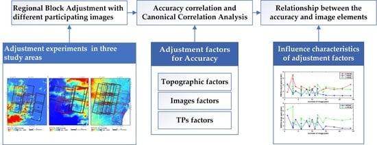
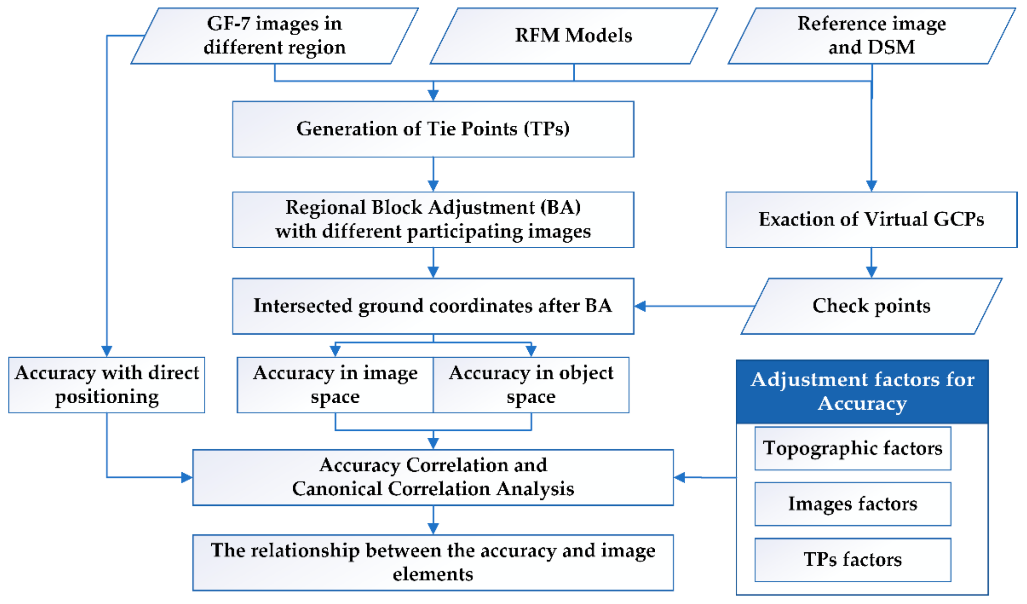
2. Study Areas and Data Sources
3. Methods
3.1. Regional Block Adjustments of Stereo Images Using RFM
3.2. Validation of Accuracy
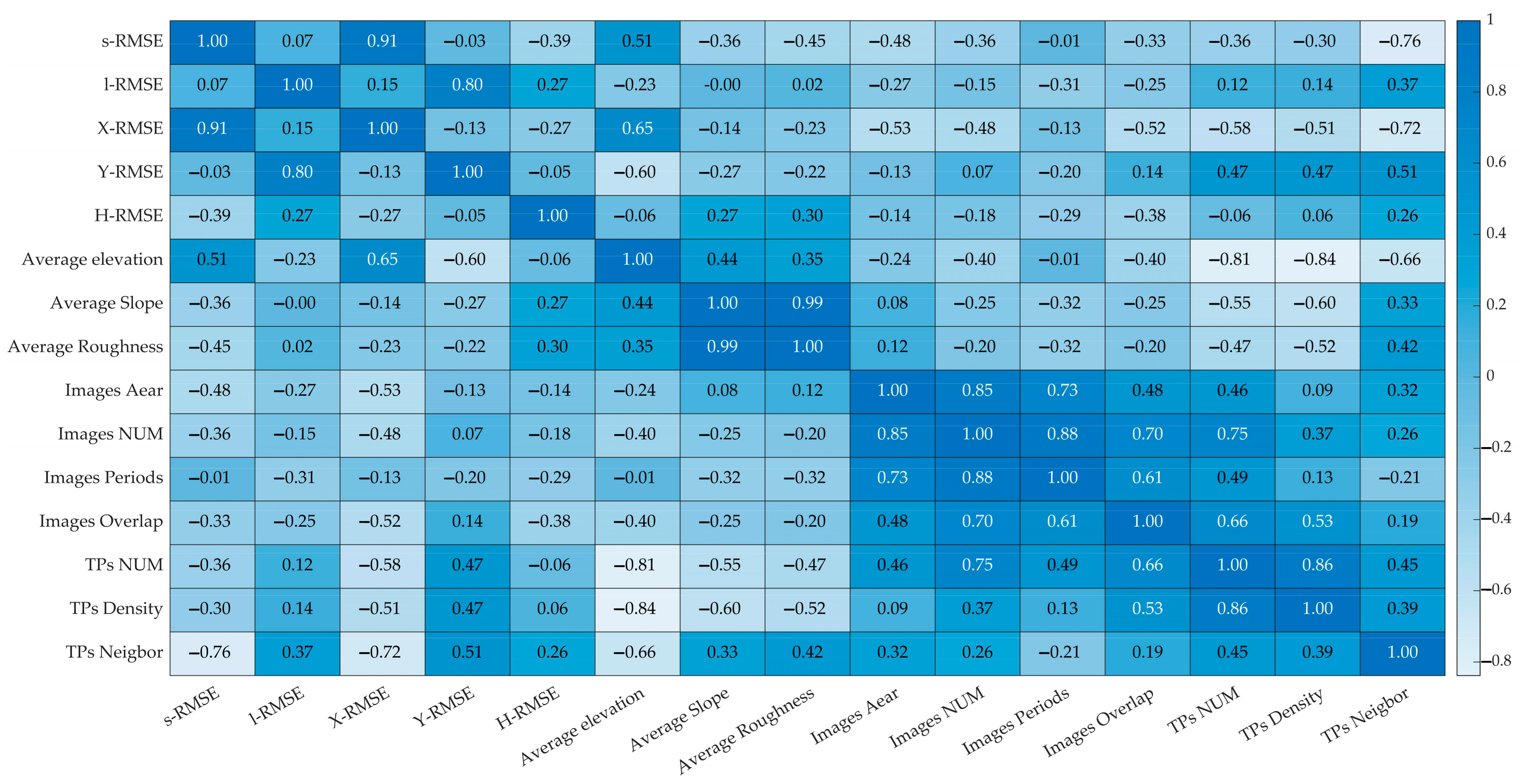
3.3. Accuracy Correlation Coefficient and Canonical Correlation Analysis
3.4. Selection of Block Adjustment Factors
4. Results
4.1. Accuracy of Regional Block Adjustments
4.2. Correlation Coefficients between the Accuracy Indicators and Adjustment Factors
4.3. Relationship from Canonical Correlation Analysis
4.4. Different Combinations of Regional Block Adjustments
5. Discussion
5.1. Influence Characteristics of Adjustment Factors on the Accuracy
5.2. Influence of Non-Adjustment Factors on Accuracy
6. Conclusions
- (1)
- The positioning accuracy does not deteriorate with time for GF-7 satellite imagery. The RFM-based regional block adjustment without GCPs can improve the direct positioning accuracy for GF-7 stereo imagery, but the improvement is affected by the factors of regional topography, the participating images, and the TPs involved in the adjustment.
- (2)
- The set of TP factors is the most influential factor set among the three sets of ten adjustment factors. Therefore, improving the quality of TPs, especially their more uniform distribution, is the key to improving the accuracy of regional block adjustment.
- (3)
- Topographic factors also play an important role in the adjustment of Gaofen-7 stereo imagery without GCPs. The influence of topographic factors on accuracy is different in different regions. Further, the influence of the elevation factor, with the highest canonical correlation coefficient (−0.71), is more significant than the other two factors.
- (4)
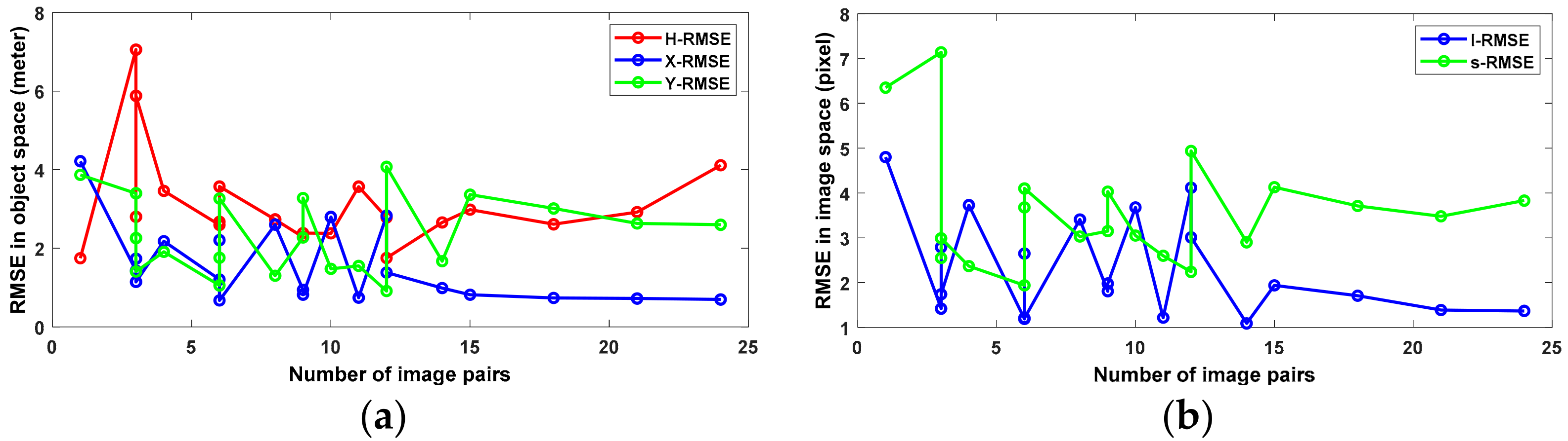
- The influence of image overlap on accuracy is more critical than the image coverage area, number, and time periods for the selection of images participating in adjustment. At the same time, the influence of image number on accuracy does not change much when the number of images exceeds a certain number (15 pairs) for GF-7 images. In other words, under the condition that the overlap of images is satisfied, this is of great referential significance for the partition processing of large-area block adjustment for GF-7 stereo imagery.
- (5)
- The five accuracy indicators used in this paper can reflect the level of adjustment accuracy, but the influence of three sets of factors is different. The ten adjustment factors have less influence on the accuracy of image space, especially the direction in image space, which is related to the physical characteristics of the image from the camera. This can be inferred from the fact that its improvement requires the internal inspection and correction of the images, or from the unknown reflected in the regional block adjustment.
Author Contributions
Funding
Data Availability Statement
Acknowledgments
Conflicts of Interest
Appendix A

| Experimental Serial Number | The Set of Regional Topographic Factors | The Set of Participating Image Factors | The Set of Image TPs Factors | |||||||
|---|---|---|---|---|---|---|---|---|---|---|
| Average Elevation | Average Slope | Average Roughness | Images Area | Images Number | Images Periods | Degree of Images Overlap | TPs Number | TPs Density | TPs Nearest Neighbor Coefficient | |
| (1) | 69.55 | 7.48 | 11.28 | 59,601.00 | 14 | 5 | 47.61% | 1263 | 0.212 | 0.60 |
| (2) | 92.51 | 9.44 | 14.07 | 4277.03 | 11 | 4 | 58.86% | 1072 | 0.251 | 0.58 |
| (3) | 99.08 | 9.75 | 14.54 | 3813.39 | 9 | 3 | 46.22% | 809 | 0.212 | 0.59 |
| (4) | 112.20 | 10.74 | 16.06 | 2221.78 | 6 | 2 | 66.84% | 509 | 0.229 | 0.61 |
| (5) | 121.47 | 11.13 | 16.60 | 1645.40 | 3 | 1 | 9.22% | 246 | 0.15 | 0.65 |
| (6) | 173.07 | 4.77 | 6.56 | 2983.67 | 12 | 7 | 68.36% | 1118 | 0.375 | 0.34 |
| (7) | 171.45 | 4.75 | 6.52 | 2956.36 | 10 | 6 | 61.51% | 1111 | 0.376 | 0.35 |
| (8) | 156.97 | 4.57 | 6.28 | 2711.86 | 8 | 5 | 37.67% | 1065 | 0.393 | 0.35 |
| (9) | 102.21 | 4.01 | 5.52 | 1846.39 | 6 | 4 | 45.85% | 726 | 0.393 | 0.38 |
| (10) | 106.00 | 4.16 | 5.72 | 1671.29 | 4 | 3 | 38.37% | 572 | 0.342 | 0.37 |
| (11) | 88.28 | 3.82 | 5.26 | 1466.91 | 3 | 2 | 27.20% | 265 | 0.181 | 0.47 |
| (12) | 84.71 | 3.82 | 5.23 | 701.92 | 1 | 1 | 0 | 152 | 0.217 | 0.49 |
| (13) | 10.02 | 2.99 | 4.89 | 5666.49 | 24 | 8 | 70.77% | 6023 | 1.063 | 0.57 |
| (14) | 10.24 | 3.26 | 5.34 | 4057.01 | 21 | 7 | 92.93% | 5839 | 1.439 | 0.59 |
| (15) | 10.26 | 3.29 | 5.38 | 3912.78 | 18 | 6 | 81.43% | 5638 | 1.441 | 0.59 |
| (16) | 10.42 | 3.46 | 5.66 | 3267.32 | 15 | 5 | 84.66% | 5233 | 1.602 | 0.61 |
| (17) | 10.50 | 3.55 | 5.81 | 3022.01 | 12 | 4 | 90.57% | 5036 | 1.666 | 0.60 |
| (18) | 10.50 | 3.55 | 5.81 | 3022.01 | 9 | 3 | 61.95% | 5036 | 1.666 | 0.60 |
| (19) | 10.17 | 3.53 | 5.79 | 1733.50 | 6 | 2 | 93.91% | 2971 | 1.714 | 0.55 |
| (20) | 10.11 | 3.52 | 5.77 | 1667.33 | 3 | 1 | 10.68% | 2965 | 1.778 | 0.56 |
| Experimental Serial Number | Accuracy Indicators | ||||
|---|---|---|---|---|---|
| -RMSE (Pixel) | -RMSE (Pixel) | -RMSE (m) | -RMSE (m) | -RMSE (m) | |
| (1) | 1.09 | 2.9 | 0.99 | 1.672 | 2.658 |
| (2) | 1.22 | 2.6 | 0.746 | 1.552 | 3.57 |
| (3) | 1.81 | 3.15 | 0.945 | 2.273 | 2.289 |
| (4) | 1.19 | 1.94 | 1.205 | 1.055 | 2.595 |
| (5) | 1.42 | 7.14 | 1.432 | 3.400 | 7.053 |
| (6) | 4.12 | 2.24 | 2.830 | 0.913 | 2.782 |
| (7) | 3.68 | 3.05 | 2.797 | 1.479 | 2.381 |
| (8) | 3.41 | 3.03 | 2.603 | 1.303 | 2.735 |
| (9) | 2.65 | 3.68 | 2.208 | 1.759 | 2.675 |
| (10) | 3.73 | 2.37 | 2.181 | 1.909 | 3.461 |
| (11) | 2.79 | 2.55 | 1.736 | 2.260 | 2.8 |
| (12) | 4.80 | 6.35 | 4.216 | 3.869 | 1.748 |
| (13) | 1.37 | 3.83 | 0.698 | 2.598 | 4.113 |
| (14) | 1.39 | 3.48 | 0.723 | 2.631 | 2.922 |
| (15) | 1.71 | 3.71 | 0.738 | 3.013 | 2.611 |
| (16) | 1.94 | 4.13 | 0.82 | 3.363 | 2.983 |
| (17) | 3.01 | 4.94 | 1.385 | 4.072 | 1.753 |
| (18) | 1.98 | 4.03 | 0.821 | 3.279 | 2.387 |
| (19) | 1.21 | 4.1 | 0.674 | 3.265 | 3.571 |
| (20) | 1.74 | 2.99 | 1.145 | 1.409 | 5.879 |
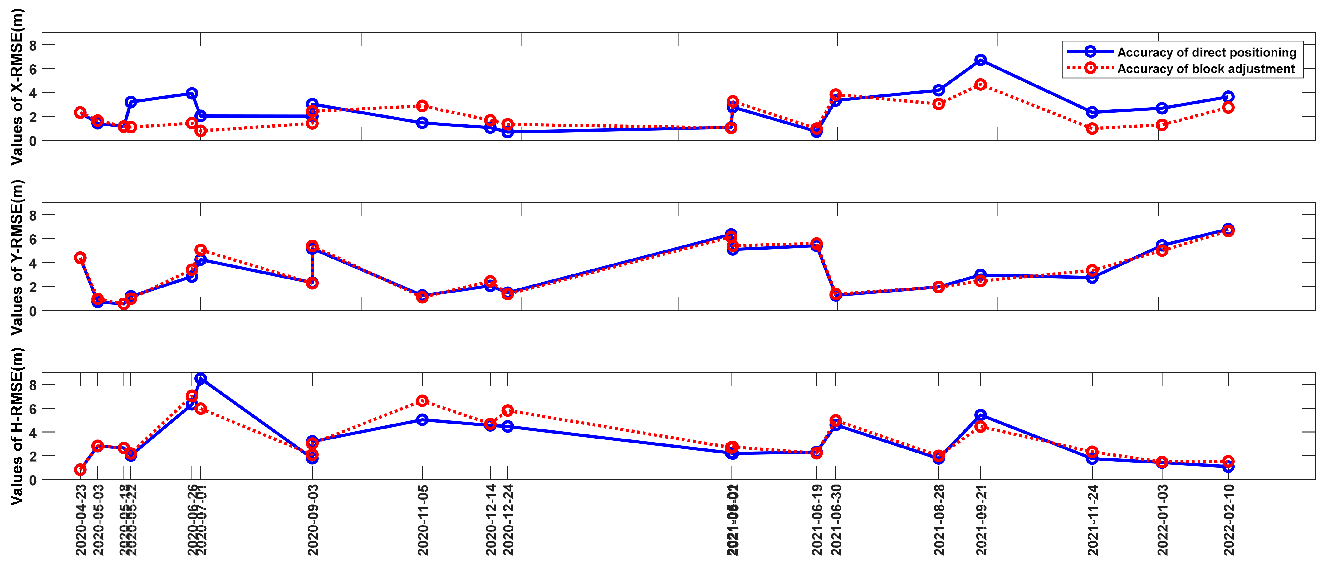
| Period of Images | Acquisition Time of Images | Central Latitude and Longitude of Images | Accuracy of Direct Stereo Positioning | Accuracy of Block Adjustment in Each Single Time Period | ||||
|---|---|---|---|---|---|---|---|---|
| X-RMSE (m) | Y-RMSE (m) | H-RMSE (m) | X-RMSE (m) | Y-RMSE (m) | H-RMSE (m) | |||
| H1 | 2020-06-26 3 pairs (6 scenes) | E119.5_N30.7 | 3.750 | 2.894 | 6.621 | 1.432 | 3.400 | 7.053 |
| E119.6_N30.9 | 3.939 | 2.736 | 7.950 | |||||
| E119.6_N31.1 | 4.069 | 2.838 | 4.414 | |||||
| H2 | 2021-11-24 3 pairs (6 scenes) | E119.6_N30.7 | 2.664 | 2.897 | 2.248 | 0.984 | 3.343 | 2.319 |
| E119.6_N30.9 | 1.778 | 3.063 | 1.636 | |||||
| E119.7_N31.1 | 2.583 | 2.250 | 1.372 | |||||
| H3 | 2022-01-03 3 pairs (6 scenes) | E119.9_N30.7 | 2.425 | 5.891 | 1.584 | 1.291 | 4.991 | 1.465 |
| E119.9_N30.9 | 2.531 | 5.291 | 1.433 | |||||
| E119.9_N31.1 | 3.075 | 5.122 | 1.232 | |||||
| H4 | 2020-09-03 2 pairs (4 scenes) | E120.0_N30.7 | 1.864 | 2.361 | 2.130 | 1.414 | 2.259 | 2.083 |
| E120.0_N30.9 | 2.160 | 2.267 | 1.427 | |||||
| H5 | 2020-05-03 3 pairs (6 scenes) | E120.2_N30.7 | 1.404 | 0.774 | 2.694 | 1.653 | 0.953 | 2.819 |
| E120.1_N30.5 | 1.481 | 0.662 | 2.385 | |||||
| E120.2_N30.9 | 1.385 | 0.691 | 3.337 | |||||
| Period of Images | Acquisition Time | Central Latitude and Longitude of Images | Accuracy of Direct Stereo Positioning | Accuracy of Block Adjustment in Each Single Time Period | ||||
|---|---|---|---|---|---|---|---|---|
| X-RMSE (m) | Y-RMSE (m) | H-RMSE (m) | X-RMSE (m) | Y-RMSE (m) | H-RMSE (m) | |||
| M1 | 2020-04-23 1 pair (2 scenes) | E4.9_N43.7 | 2.321 | 4.395 | 0.817 | 2.321 | 4.395 | 0.817 |
| M2 | 2020-07-01 2 pairs (4 scenes) | E5.1_N43.7 | 1.689 | 3.708 | 9.677 | 0.786 | 5.049 | 5.970 |
| E5.0_N43.5 | 2.378 | 4.763 | 7.339 | |||||
| M3 | 2020-05-18 1 pair (2 scenes) | E5.2_N43.7 | 1.153 | 0.538 | 2.645 | 1.153 | 0.538 | 2.645 |
| M4 | 2020-09-03 2 pairs (4 scenes) | E5.2_N43.7 | 3.637 | 5.219 | 4.377 | 2.432 | 5.377 | 3.0169 |
| E5.1_N43.5 | 2.415 | 5.097 | 2.028 | |||||
| M5 | 2021-08-28 2 pairs (4 scenes) | E5.3_N43.5 | 3.813 | 1.336 | 2.535 | 3.034 | 1.938 | 1.988 |
| E5.4_N43.7 | 4.549 | 2.570 | 1.003 | |||||
| M6 | 2021-06-30 2 pairs (4 scenes) | E5.4_N43.7 | 3.678 | 0.903 | 3.974 | 3.827 | 1.354 | 4.972 |
| E5.4_N43.5 | 2.980 | 1.612 | 5.208 | |||||
| M7 | 2021-05-02 2 pairs (4 scenes) | E5.4_N43.5 | 2.463 | 5.641 | 3.139 | 3.248 | 5.404 | 2.733 |
| E5.5_N43.7 | 3.085 | 4.538 | 1.224 | |||||
| Period of Images | Acquisition Time | Central Latitude and Longitude of Images | Accuracy of Direct Stereo Positioning | Accuracy of Block Adjustment at Each Single Time Period | ||||
|---|---|---|---|---|---|---|---|---|
| X-RMSE (m) | Y-RMSE (m) | H-RMSE (m) | X-RMSE (m) | Y-RMSE (m) | H-RMSE (m) | |||
| T1 | 2020-12-24 3 pairs (6 scenes) | E116.9_N39.0 | 0.484 | 1.679 | 3.706 | 1.341 | 1.354 | 5.803 |
| E117.0_N39.2 | 0.676 | 1.836 | 6.259 | |||||
| E117.0_N39.4 | 0.912 | 0.891 | 3.429 | |||||
| T2 | 2021-06-19 3 pairs (6 scenes) | E116.9_N39.0 | 0.661 | 5.407 | 0.990 | 0.979 | 5.584 | 2.209 |
| E117.0_N39.4 | 0.714 | 5.078 | 3.413 | |||||
| E116.9_N39.2 | 0.835 | 5.729 | 2.525 | |||||
| T3 | 2021-09-21 3 pairs (6 scenes) | E117.1_N39.0 | 7.310 | 2.844 | 6.836 | 4.666 | 2.453 | 4.457 |
| E117.1_N39.2 | 6.711 | 3.154 | 5.504 | |||||
| E117.2_N39.4 | 6.121 | 2.891 | 3.971 | |||||
| T4 | 2022-02-10 3 pairs (6 scenes) | E117.1_N39.0 | 3.898 | 6.975 | 0.746 | 2.750 | 6.630 | 1.521 |
| E117.1_N39.2 | 3.914 | 7.308 | 1.226 | |||||
| E117.2_N39.4 | 3.101 | 6.059 | 1.268 | |||||
| T5 | 2020-12-14 3 pairs (6 scenes) | E117.1_N39.0 | 0.833 | 1.838 | 4.550 | 1.679 | 2.424 | 4.684 |
| E117.2_N39.4 | 1.399 | 2.051 | 4.913 | |||||
| E117.2_N39.2 | 0.927 | 2.236 | 4.190 | |||||
| T6 | 2020-05-22 3 pairs (6 scenes) | E117.2_N39.0 | 3.043 | 0.839 | 2.011 | 1.100 | 0.971 | 2.185 |
| E117.3_N39.2 | 3.224 | 1.013 | 1.568 | |||||
| E117.3_N39.4 | 3.333 | 1.641 | 2.481 | |||||
| T7 | 2020-11-05 3 pairs (6 scenes) | E117.3_N39.2 | 1.383 | 1.511 | 4.153 | 2.869 | 1.087 | 6.632 |
| E117.4_N39.4 | 1.555 | 1.050 | 6.901 | |||||
| E117.3_N39.0 | 1.450 | 1.167 | 4.038 | |||||
| T8 | 2021-05-01 3 pairs (6 scenes) | E117.5_N39.0 | 1.186 | 5.809 | 2.681 | 1.031 | 6.137 | 2.687 |
| E117.4_N38.8 | 0.938 | 6.088 | 1.894 | |||||
| E117.6_N39.2 | 1.095 | 7.128 | 2.093 | |||||
References
- Cao, H.; Tao, P.; Liu, Y.; Li, H. Nonlinear Systematic Distortions Compensation in Satellite Images Based on an Equivalent Geometric Sensor Model Recovered From RPCs. IEEE J. Sel. Top. Appl. Earth Obs. Remote Sens. 2021, 14, 12088–12102. [Google Scholar] [CrossRef]
- Radhadevi, P.V.; Müller, R.; d’Angelo, P.; Reinartz, P. In-flight Geometric Calibration and Orientation of ALOS/PRISM Imagery with a Generic Sensor Model. Photogramm. Eng. Remote Sens. 2011, 77, 531–538. [Google Scholar] [CrossRef]
- Takaku, J.; Tadono, T. RPC generations on ALOS PRISM and AVNIR-2. In Proceedings of the IEEE International Geoscience and Remote Sensing Symposium (IGARSS), Vancouver, BC, Canada, 24–29 July 2011. [Google Scholar]
- Tang, X.; Zhou, P.; Zhang, G.; Wang, X.; Pan, H. Geometric Accuracy Analysis Model of the Ziyuan-3 Satellite without GCPs. Photogramm. Eng. Remote Sens. 2015, 81, 927–934. [Google Scholar] [CrossRef]
- Toutin, T. Geometric processing of remote sensing images: Models, algorithms and methods. Int. J. Remote Sens. 2010, 25, 1893–1924. [Google Scholar] [CrossRef]
- Valadan Zoej, M.J.; Mokhtarzade, M.; Mansourian, A.; Ebadi, H.; Sadeghian, S. Rational function optimization using genetic algorithms. Int. J. Appl. Earth Obs. Geoinf. 2007, 9, 403–413. [Google Scholar] [CrossRef]
- Yang, B.; Wang, M.; Xu, W.; Li, D.; Gong, J.; Pi, Y. Large-scale block adjustment without use of ground control points based on the compensation of geometric calibration for ZY-3 images. ISPRS J. Photogramm. Remote Sens. 2017, 134, 1–14. [Google Scholar] [CrossRef]
- Zhang, Y.; Lu, Y.; Wang, L.; Huang, X. A New Approach on Optimization of the Rational Function Model of High-Resolution Satellite Imagery. IEEE Trans. Geosci. Remote Sens. 2012, 50, 2758–2764. [Google Scholar] [CrossRef]
- Gong, J.; Wang, M.; Yang, B. High-precision Geometric Processing Theory and Method of High-Resolution Optical Remote Sensing Satellite Imagery without GCP. Acta Geod. Cartograph. Sin. 2017, 46, 1255–1261. [Google Scholar]
- Zhang, Y.; Wan, Y.; Shi, W.; Zhang, Z.; Li, Y.; Ji, S.; Gu, H.; Li, L. Technical Framework and Preliminary Practices of Photogrammetric Remote Sensing Intelligent Processing of Multi-Source Satellite Images. Acta Geod. Cartograph. Sin. 2021, 50, 1068–1083. [Google Scholar]
- Zhang, L.; Liu, Y.; Sun, Y.; Lan, C.; Ai, H.; Fan, Z. A Review of Developments in the Theory and Technology of Three-Dimentional Reconstruction in Digital Areial Photogrammetry. Acta Geod. Cartograph. Sin. 2022, 51, 1437–1457. [Google Scholar]
- Yang, B.; Wang, M.; Pi, Y. Block Adjustment without GCPs for Large-scale Regions only Based on the Virtual Control Points. Acta Geod. Cartograph. Sin. 2017, 46, 874–881. [Google Scholar]
- Zheng, M.; Zhang, Y.; Zhou, S.; Zhu, J.; Xiong, X. Bundle block adjustment of large-scale remote sensing data with Block-based Sparse Matrix Compression combined with Preconditioned Conjugate Gradient. Comput. Geosci. 2016, 92, 70–78. [Google Scholar] [CrossRef]
- Aurélie, B.; Marc, B.; Patrick, G.; Alain, O.; Véronique, R.; Alain, B. SPOT 5 HRS geometric performances: Using block adjustment as a key issue to improve quality of DEM generation. ISPRS J. Photogramm. Remote Sens. 2006, 60, 134–146. [Google Scholar]
- Liu, B.; Jia, M.; Di, K.; Oberst, J.; Xu, B.; Wan, W. Geopositioning precision analysis of multiple image triangulation using LROC NAC lunar images. Planet. Space Sci. 2018, 162, 20–30. [Google Scholar] [CrossRef]
- Tao, P.; Xi, K.; Niu, Z.; Chen, Q.; Liao, Y.; Liu, Y.; Liu, K.; Zhang, Z. Optimal selection from extremely redundant satellite images for efficient large-scale mapping. ISPRS J. Photogramm. Remote Sens. 2022, 194, 21–38. [Google Scholar] [CrossRef]
- Wang, C.; Sun, Z.; Liang, Z.; Zhang, J. Refined Identification of Winter Wheat Area Based on GF-7 Satellite Remote Sensing. J. Anhui Agric. Sci. 2021, 49, 244–247, 252. [Google Scholar]
- Li, G.; Tang, X. Accuracy evaluation of large lake water level measurement based on GF-7 laser altimetry data. Natl. Remote Sens. Bull. 2022, 26, 138–147. [Google Scholar]
- Luo, H.; He, B.A.; Guo, R.; Wang, W.; Kuai, X.; Xia, B.; Wan, Y.; Ma, D.; Xie, L. Urban Building Extraction and Modeling Using GF-7 DLC and MUX Images. Remote Sens. 2021, 13, 3414. [Google Scholar] [CrossRef]
- Zhang, C.; Cui, Y.; Zhu, Z.; Jiang, S.; Jiang, W. Building Height Extraction from GF-7 Satellite Images Based on Roof Contour Constrained Stereo Matching. Remote Sens. 2022, 15, 7. [Google Scholar] [CrossRef]
- Wang, J.; Hu, X.; Meng, Q.; Zhang, L.; Wang, C.; Liu, X.; Zhao, M. Developing a Method to Extract Building 3D Information from GF-7 Data. Remote Sens. 2021, 13, 4532. [Google Scholar] [CrossRef]
- Chen, C.; Ding, J.; Wang, S.; Liu, J. High-precision control technology and on-orbit verification of GF-7 satellite. Chin. Space Sci. Technol. 2020, 40, 34–41. [Google Scholar]
- Zhou, P.; Tang, X. Geometric Accuracy Verification of GF-7 Satellite Stereo Imagery Without GCPs. IEEE Geosci. Remote Sens. Lett. 2022, 19, 1–5. [Google Scholar] [CrossRef]
- Xie, Y.; Gui, M. DEM Production Based on GF-7 Stereo Pairs and The Accuracy Verification. Surv. Mapp. 2021, 44, 163–165. [Google Scholar]
- Hu, L.; Tang, X.; Zhang, Z.; Li, G.; Chen, J.; Tian, H.; Zhang, S.; Qiao, J.; Li, X. Accuracy Optimization and Assessment of GF-7 Satellite Multi-source Remote Sensing Data. Infrared Laser Eng. 2022, 51, 1–9. [Google Scholar]
- Chen, J.; Tang, X.; Xue, Y.; Li, G.; Zhou, X.; Hu, L.; Zhang, S. Registration and Combined Adjustment for the Laser Altimetry Data and High-Resolution Optical Stereo Images of the GF-7 Satellite. Remote Sens. 2022, 14, 1666. [Google Scholar] [CrossRef]
- Pi, Y.; Yang, B.; Li, X.; Wang, M. Robust Correction of Relative Geometric Errors Among GaoFen-7 Regional Stereo Images Based on Posteriori Compensation. IEEE J. Sel. Top. Appl. Earth Obs. Remote Sens. 2022, 15, 3224–3234. [Google Scholar] [CrossRef]
- Zhu, X.; Tang, X.; Zhang, G.; Liu, B.; Hu, W. Accuracy Comparison and Assessment of DSM Derived from GFDM Satellite and GF-7 Satellite Imagery. Remote Sens. 2021, 13, 4791. [Google Scholar] [CrossRef]
- Song, J.; Fan, D.; Ji, S.; Li, D.; Chu, G. Laser Spot Centroid Extraction of GF-7 Footprint Images. J. Geomat. Sci. Technol. 2021, 38, 507–513. [Google Scholar]
- Luo, H.; He, B.; Guo, R.; Wang, W.; Kuai, X.; Xia, B. GF-7 image quality assessment and interpretability analysis. Eng. Surv. Mapp. 2022, 31, 1–7. [Google Scholar]
- Tang, X.; Xie, J.; Liu, R.; Huang, G.; Zhao, C.; Zhen, Y.; Tang, H.; Dou, X. Overview of the GF-7 Laser Altimeter System Mission. Earth Space Sci. 2020, 7, 1. [Google Scholar] [CrossRef]
- Si, S.; Sun, X. Mathematical Modeling; National Defense Industry Press: Beijing, China, 2014. [Google Scholar]
- Tachikawa, T.; Hato, M.; Kaku, M. Characteristics of ASTER GDEM version 2. In Proceedings of the IEEE International Geoscience and Remote Sensing Symposium (IGARSS), Vancouver, BC, Canada, 24–29 July 2011. [Google Scholar]
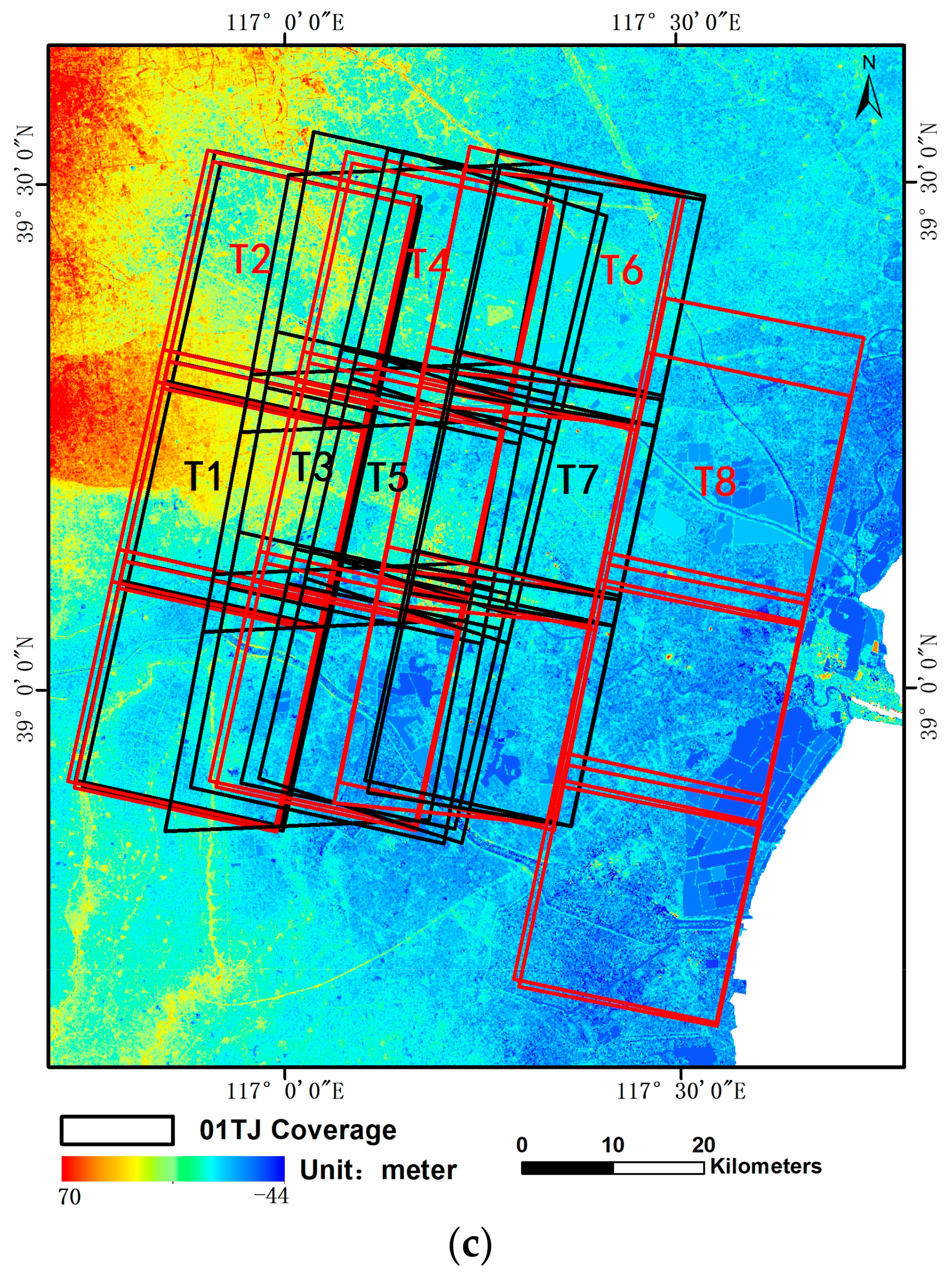
| 08HZ Region | 07MS Region | 01TJ Region | |||
|---|---|---|---|---|---|
| Period of Images | Acquisition Time and Quantity of Images | Period of Images | Acquisition Time and Quantity of Images | Period of Images | Acquisition Time and Quantity of Images |
| H1 | 26 June 2020 3 pairs (6 scenes) | M1 | 23 April 2020 1 pair (2 scenes) | T1 | 24 December 2020 3 pairs (6 scenes) |
| H2 | 24 November 2021 3 pairs (6 scenes) | M2 | 1 July 2020 2 pairs (4 scenes) | T2 | 19 June 2021 3 pairs (6 scenes) |
| H3 | 3 January 2022 3 pairs (6 scenes) | M3 | 18 May 2020 1 pair (2 scenes) | T3 | 21 September 2021 3 pairs (6 scenes) |
| H4 | 3 September 2020 2 pairs (4 scenes) | M4 | 3 September 2020 2 pairs (4 scenes) | T4 | 10 February 2022 3 pairs (6 scenes) |
| H5 | 3 May 2020 3 pairs (6 scenes) | M5 | 28 August 2021 2 pairs (4 scenes) | T5 | 14 December 2020 3 pairs (6 scenes) |
| M6 | 30 June 2021 2 pairs (4 scenes) | T6 | 22 May 2020 3 pairs (6 scenes) | ||
| M7 | 2 May 2021 2 pairs (4 scenes) | T7 | 5 November 2020 3 pairs (6 scenes) | ||
| T8 | 1 May 2021 3 pairs (6 scenes) | ||||
| Region | Average Residuals with Direct Stereo Positioning before Block Adjustment (Meter) | Average Residuals after Block Adjustment for Each Single Period (Meter) | Residuals after Block Adjustment with All Images in this Region (Meter) | ||||||
|---|---|---|---|---|---|---|---|---|---|
| X-RMSE | Y-RMSE | H-RMSE | X-RMSE | Y-RMSE | H-RMSE | X-RMSE | Y-RMSE | H-RMSE | |
| 08HZ | 2.51 | 2.84 | 2.89 | 1.35 | 2.99 | 3.15 | 0.99 | 1.67 | 2.66 |
| 07MS | 2.85 | 3.36 | 3.66 | 2.40 | 3.44 | 3.16 | 2.83 | 0.91 | 2.78 |
| 01TJ | 2.32 | 3.43 | 3.39 | 2.05 | 3.33 | 3.77 | 0.70 | 2.60 | 4.11 |
| Average | 2.56 | 3.21 | 3.31 | 1.93 | 3.25 | 3.36 | 1.51 | 1.73 | 3.18 |
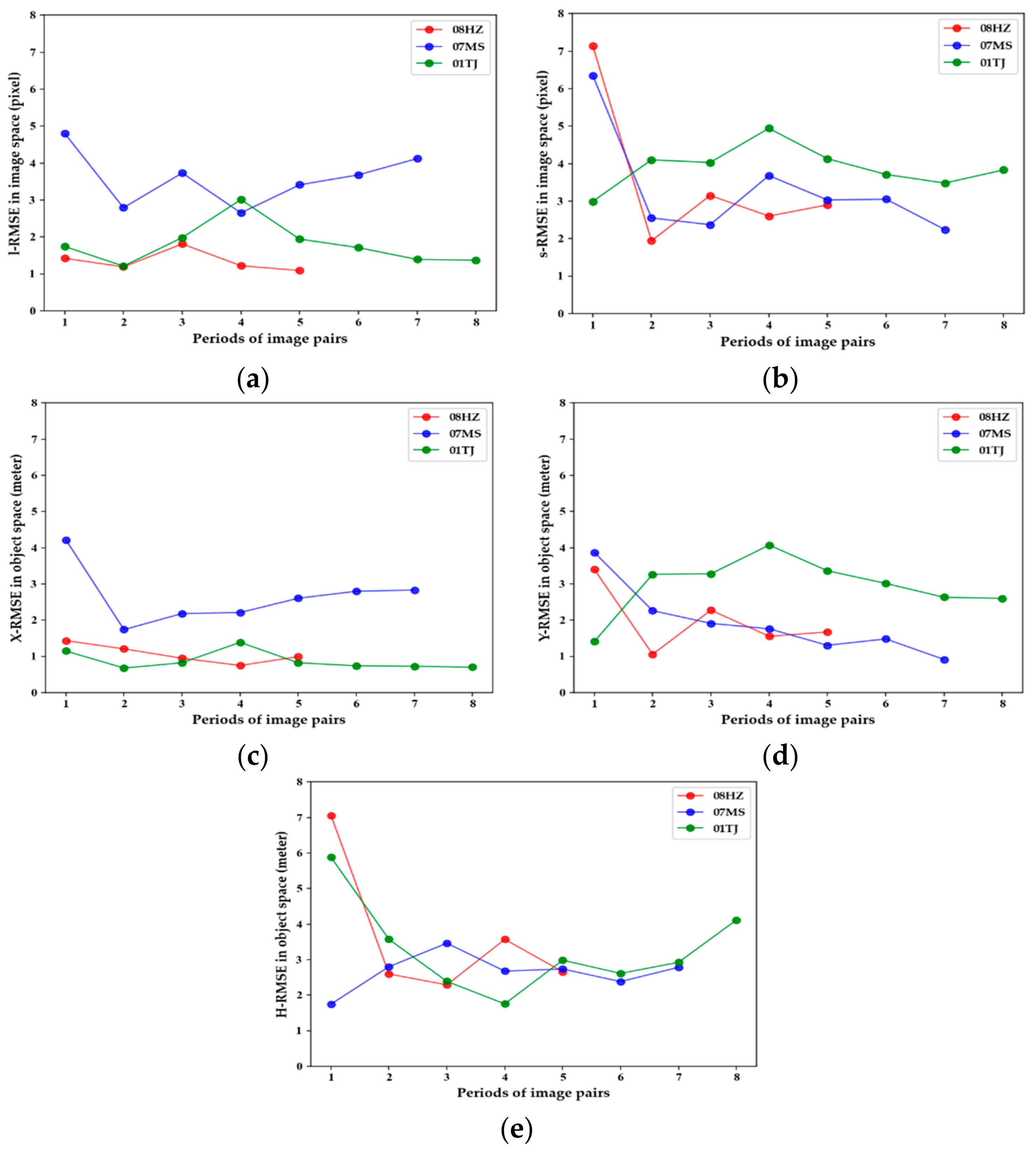
| Periods of Participated Images | Number of Images Pairs | Residuals in Image Space (Pixel) | Residuals in Object Space (Meter) | |||
|---|---|---|---|---|---|---|
| s-RMSE | l-RMSE | X-RMSE | Y-RMSE | H-RMSE | ||
| 5 (H1 H2 H3 H4 H5) | 14 | 1.09 | 2.90 | 0.99 | 1.67 | 2.66 |
| 4 (H1 H2 H3 H4) | 11 | 1.22 | 2.60 | 0.75 | 1.55 | 3.57 |
| 3 (H1 H2 H3) | 9 | 1.81 | 3.15 | 0.95 | 2.27 | 2.29 |
| 2 (H1 H2) | 6 | 1.19 | 1.94 | 1.21 | 1.06 | 2.60 |
| 1 (H1) | 3 | 1.42 | 7.14 | 1.43 | 3.40 | 7.05 |
| Periods of Participated Images | Number of Images Pairs | Residuals in Image Space (Pixel) | Residuals in Object Space (Meter) | |||
|---|---|---|---|---|---|---|
| s-RMSE | l-RMSE | X-RMSE | Y-RMSE | H-RMSE | ||
| 7 (M1M2M3M4M5M6M7) | 14 | 4.12 | 2.24 | 2.83 | 0.91 | 2.78 |
| 6 (M1M2M3M4M5M6) | 12 | 3.68 | 3.05 | 2.80 | 1.48 | 2.38 |
| 5 (M1M2M3M4M5) | 8 | 3.41 | 3.03 | 2.60 | 1.30 | 2.74 |
| 4 (M1M2M3M4) | 6 | 2.65 | 3.68 | 2.21 | 1.76 | 2.68 |
| 3 (M1M2M3) | 4 | 3.73 | 2.37 | 2.18 | 1.91 | 3.46 |
| 2 (M1M2) | 3 | 2.79 | 2.55 | 1.74 | 2.26 | 2.80 |
| 1 (M1) | 1 | 4.80 | 6.35 | 4.22 | 3.87 | 1.75 |
| Periods of Participated Images | Number of Images Pairs | Residuals in Image Space (Pixel) | Residuals in Object Space (Meter) | |||
|---|---|---|---|---|---|---|
| s-RMSE | l-RMSE | X-RMSE | Y-RMSE | H-RMSE | ||
| 8 (T1T2T3T4T5T6T7T8) | 24 | 1.37 | 3.83 | 0.70 | 2.60 | 4.11 |
| 7 (T1T2T3T4T5T6T7) | 21 | 1.39 | 3.48 | 0.72 | 2.63 | 2.92 |
| 6 (T1T2T3T4T5T6) | 18 | 1.71 | 3.71 | 0.74 | 3.01 | 2.61 |
| 5 (T1T2T3T4T5) | 15 | 1.94 | 4.13 | 0.82 | 3.36 | 2.98 |
| 4 (T1T2T3T4) | 12 | 3.01 | 4.94 | 1.39 | 4.07 | 1.75 |
| 3 (T1T2T3) | 9 | 1.98 | 4.03 | 0.82 | 3.28 | 2.39 |
| 2 (T1T2) | 6 | 1.21 | 4.10 | 0.67 | 3.27 | 3.57 |
| 1 (T1) | 3 | 1.74 | 2.99 | 1.15 | 1.41 | 5.88 |
| Serial Number | 1 | 2 | 3 | 4 | 5 |
|---|---|---|---|---|---|
| Canonical correlation coefficients | 0.99 | 0.94 | 0.92 | 0.74 | 0.57 |
| Degree of Freedom | 50 | 36 | 24 | 14 | 6 |
| Calculated value of | 105.84 | 58.48 | 34.26 | 13.47 | 4.87 |
| Critical value of (significance level is 0.05) | 0.0000070 | 0.010 | 0.080 | 0.49 | 0.56 |
| The set of regional topographic factors | Average elevation | −0.71 | −0.35 | −0.71 | 0.33 |
| Average slope | −0.32 | 0.32 | −0.31 | −0.30 | |
| Average roughness | −0.26 | 0.40 | −0.26 | −0.37 | |
| The set of participating image factors | Images area | 0.11 | 0.70 | 0.11 | −0.66 |
| Images number | 0.24 | 0.59 | 0.24 | −0.55 | |
| Images periods | −0.06 | 0.35 | −0.064 | −0.33 | |
| Images overlap degree | 0.48 | 0.50 | 0.47 | −0.47 | |
| The set of image TPs factors | TPs number | 0.52 | 0.49 | 0.51 | −0.46 |
| TPs density | 0.48 | 0.34 | 0.48 | −0.33 | |
| TPs nearest neighbor coefficient | 0.50 | 0.58 | 0.50 | −0.55 | |
| Accuracy indicators in image space | -RMSE | −0.24 | 0.78 | −0.24 | −0.74 |
| -RMSE | 0.16 | 0.14 | 0.16 | −0.13 | |
| Accuracy indicators in object space | -RMSE | −0.39 | 0.83 | −0.39 | −0.79 |
| -RMSE | 0.68 | 0.066 | 0.67 | −0.062 | |
| -RMSE | −0.45 | −0.24 | −0.45 | 0.22 | |
| Region | Periods of Participated Images | TPs Number | Residuals in Image Space (Pixel) | Residuals in Object Space (Meter) | |||
|---|---|---|---|---|---|---|---|
| s-RMSE | l-RMSE | X-RMSE | Y-RMSE | H-RMSE | |||
| 08HZ | 5 (H1 H2 H3 H4 H5) | 1 multiple | 1.09 | 2.90 | 0.99 | 1.67 | 2.66 |
| 5 (H1 H2 H3 H4 H5) | 2 multiples | 1.22 | 2.60 | 0.95 | 1.37 | 2.08 | |
| 5 (H1 H2 H3 H4 H5) | 4 multiples | 1.11 | 1.91 | 0.83 | 1.28 | 1.87 | |
| 07MS | 7 (M1M2M3M4M5M6M7) | 1 multiple | 4.12 | 2.24 | 2.83 | 0.91 | 2.78 |
| 7 (M1M2M3M4M5M6M7) | 2 multiples | 4.28 | 2.04 | 2.961 | 0.84 | 2.14 | |
| 7 (M1M2M3M4M5M6M7) | 4 multiples | 4.76 | 1.89 | 3.262 | 0.37 | 3.22 | |
| 01TJ | 8 (T1T2T3T4T5T6T7T8) | 1 multiple | 1.37 | 3.83 | 0.70 | 2.60 | 4.11 |
| 8 (T1T2T3T4T5T6T7T8) | 2 multiples | 1.82 | 3.48 | 1.04 | 2.61 | 3.46 | |
| 8 (T1T2T3T4T5T6T7T8) | 4 multiples | 1.76 | 3.51 | 1.00 | 2.62 | 3.55 | |
| Periods of Participated Images | Number of Images Pairs | Residuals in Image Space (Pixel) | Residuals in Object Space (Meter) | |||
|---|---|---|---|---|---|---|
| s-RMSE | l-RMSE | X-RMSE | Y-RMSE | H-RMSE | ||
| 4 (T1T4T7T8) | 11 | 2.07 | 5.39 | 0.77 | 3.77 | 4.83 |
| 3 (T1T4T7) | 8 | 1.94 | 4.29 | 0.82 | 3.40 | 3.17 |
| 2 (T2T4) | 6 | 1.74 | 2.99 | 1.94 | 6.29 | 2.18 |
| 2 (T2T3) | 6 | 3.75 | 5.03 | 1.92 | 4.10 | 1.36 |
| 2 (T1T4) | 6 | 2.37 | 4.81 | 0.93 | 3.95 | 3.33 |
| 2 (T1T3) | 6 | 1.71 | 3.12 | 0.79 | 2.32 | 4.25 |
| 1 (T1) | 3 | 1.74 | 2.99 | 1.15 | 1.41 | 5.88 |
| Region | Topographic Factors | Correlation Coefficients | ||||
|---|---|---|---|---|---|---|
| s-RMSE | l-RMSE | X-RMSE | Y-RMSE | H-RMSE | ||
| 08HZ | Average elevation | 0.35 | 0.52 | 0.69 | 0.44 | 0.59 |
| Average slope | 0.35 | 0.44 | 0.61 | 0.37 | 0.53 | |
| Average roughness | 0.34 | 0.44 | 0.62 | 0.36 | 0.53 | |
| 07MS | Average elevation | 0.13 | −0.47 | 0.02 | −0.77 | 0.09 |
| Average slope | 0.16 | −0.49 | 0.01 | −0.78 | 0.16 | |
| Average roughness | 0.14 | −0.51 | −0.01 | −0.79 | 0.17 | |
| 01TJ | Average elevation | 0.74 | 0.64 | 0.39 | 0.72 | −0.77 |
| Average slope | 0.48 | 0.28 | 0.51 | 0.26 | −0.14 | |
| Average roughness | 0.47 | 0.27 | 0.51 | 0.26 | −0.14 | |
Disclaimer/Publisher’s Note: The statements, opinions and data contained in all publications are solely those of the individual author(s) and contributor(s) and not of MDPI and/or the editor(s). MDPI and/or the editor(s) disclaim responsibility for any injury to people or property resulting from any ideas, methods, instructions or products referred to in the content. |
© 2023 by the authors. Licensee MDPI, Basel, Switzerland. This article is an open access article distributed under the terms and conditions of the Creative Commons Attribution (CC BY) license (https://creativecommons.org/licenses/by/4.0/).
Share and Cite
Tang, X.; Zhu, X.; Hu, W.; Ding, J. Geometric Accuracy Analysis of Regional Block Adjustment Using GF-7 Stereo Images without GCPs. Remote Sens. 2023, 15, 2552. https://doi.org/10.3390/rs15102552
Tang X, Zhu X, Hu W, Ding J. Geometric Accuracy Analysis of Regional Block Adjustment Using GF-7 Stereo Images without GCPs. Remote Sensing. 2023; 15(10):2552. https://doi.org/10.3390/rs15102552
Chicago/Turabian StyleTang, Xinming, Xiaoyong Zhu, Wenmin Hu, and Jianhang Ding. 2023. "Geometric Accuracy Analysis of Regional Block Adjustment Using GF-7 Stereo Images without GCPs" Remote Sensing 15, no. 10: 2552. https://doi.org/10.3390/rs15102552
APA StyleTang, X., Zhu, X., Hu, W., & Ding, J. (2023). Geometric Accuracy Analysis of Regional Block Adjustment Using GF-7 Stereo Images without GCPs. Remote Sensing, 15(10), 2552. https://doi.org/10.3390/rs15102552