Spatial Prediction of Soil Organic Carbon Stock in the Moroccan High Atlas Using Machine Learning

Abstract

Soil organic carbon (SOC) is an essential component, which soil quality depends on. Thus, understanding the spatial distribution and controlling factors of SOC is paramount to achieving sustainable soil management. In this study, SOC prediction for the Ourika watershed in Morocco was done using four machine learning (ML) algorithms: Cubist, random forest (RF), support vector machine (SVM), and gradient boosting machine (GBM). A total of 420 soil samples were collected at three different depths (0–10 cm, 10–20 cm, and 20–30 cm) from which SOC concentration and bulk density (BD) were measured, and consequently SOC stock (SOCS) was determined. Modeling data included 88 variables incorporating environmental covariates, including soil properties, climate, topography, and remote sensing variables used as predictors. The results showed that RF (R² = 0.79, RMSE = 1.2%) and Cubist (R² = 0.77, RMSE = 1.2%) were the most accurate models for predicting SOC, while none of the models were satisfactory in predicting BD across the watershed. As with SOC, Cubist (R² = 0.86, RMSE = 11.62 t/ha) and RF (R² = 0.79, RMSE = 13.26 t/ha) exhibited the highest predictive power for SOCS. Land use/land cover (LU/LC) was the most critical factor in predicting SOC and SOCS, followed by soil properties and bioclimatic variables. Both combinations of bioclimatic–topographic variables and soil properties–remote sensing variables were shown to improve prediction performance. Our findings show that ML algorithms can be a viable tool for spatial modeling of SOC in mountainous Mediterranean regions, such as the study area.

1. Introduction

Soil carbon sequestration plays an important role in addressing climate change [1] by mitigating the effects of greenhouse gases [2,3,4,5]. In tropical ecosystems, soil carbon stocks account for up to 60% of the total carbon in the system, which is about 1600 PgC [6,7,8]. This underscores the role of soils as reservoirs of organic carbon not only in these regions but also across the planet [9]. Soil organic carbon (SOC) is a key determinant of soil fertility and thus of agricultural potential [10,11,12]. SOC stock is related to soil water infiltration, water retention, and soil structural stability [13].

Information on the spatial distribution of SOCS in different geographical areas can be used as a basis to study soil evolution [14,15,16]. With the spatial data obtained for SOCS, monitoring soil quality, and understanding variations that may impact atmospheric carbon dioxide (CO₂) levels [12], greenhouse gas concentration and emissions, will be feasible [17]. The spatial distribution of SOCS varies with soil type, depth, climate, among others, [18]. Therefore, there are many approaches for SOCS measurement. Reflectance spectroscopy in the visible and near- and mid-infrared bands has yielded good results [13,19,20], while approaches such as Walkley and Black [21], Mebius [22], colorimetric [23], and dry burning have yielded satisfactory results in past studies despite certain limitations.

In recent years, digital soil mapping (DSM) approaches have replaced conventional methods, which are time-consuming and expensive [24]. DSM has been widely used in the prediction and subsequent mapping of the spatial variation in SOC [25,26,27]. Geostatistical methods from sampling points based on soil and environmental factors have been effective in investigating the distribution of SOCS [28,29,30,31]. The rationale for spatial prediction is that measuring SOCS at any point in space in a given area by field and laboratory work alone would be a very challenging and costly endeavor. Accordingly, spatial prediction is based on sampled points to predict the distribution of SOCS.

The recent research trend seems to be moving away from kriging as the core algorithm for mapping and toward ML for spatial prediction [32]. The DSM approach quantifies the relationships between soil properties and environmental covariates, focusing on soil-forming factors using various ML methods [24,33,34,35,36,37]. ML techniques are based on predictors to estimate the response variable such as SOCS. Typically, in DSM, environmental factors such as vegetation, climatic, and topographic variables that affect SOCS are included in addition to soil formation factors [38,39]. Both temperature and precipitation have been shown to influence SOCS [40]. In addition, vegetation parameters such as tree height, leaf area index, stem density, volume, and/or above-ground biomass have been shown to significantly influence SOCS [41,42]. Monitoring of these variables and, ultimately soil mapping, has been made possible by remote sensing techniques, as outlined by Berthier et al. [43], who studied the spatiality of SOC using visible–near-infrared spectroscopy and SPOT satellite imaging. The application of ML techniques requires that predictors go through several steps. One of these steps is variable selection, which involves limiting redundant predictors, thereby reducing computational time as well as improving model learning accuracy [44]. Several variable selection methods have been used in soil studies including LASSO, forward and backward stepwise selection techniques, sequential selection by replacement, and recursive feature elimination [45].

In low precipitation environments characterized by arid and semi-arid climates that dominate Morocco, soils are generally poor in organic matter. Thus, knowledge of the evolution of SOC is essential because it can allow management measures to be adapted according to needs, particularly in the region’s vulnerable ecosystems. The aim of this study is to predict SOC, BD, and SOCS at different soil depths (0–10 cm, 0–20 cm, and 0–30 cm) in the Ourika watershed in Morocco using ML models. Moreover, we look to identify the most important explanatory factors of SOCS in the watershed and to test if incorporating or excluding SoilGrids and WorldClim data as covariates would influence model accuracy. The objective is to provide spatial data on SOC that can serve as a resource for sustainable soil management in forests and agroecosystems.

2. Materials and Methods

2.1. Study Area

The Ourika watershed is located in the High Atlas Mountains in Morocco between latitudes 31°N and 31°20N and longitudes 7°30W and 7°60W (Figure 1). Its climate is variable, with differences in rainfall and temperature driven by factors such as altitude, topography, and proximity to the Atlantic Ocean. The higher elevations have cooler temperatures and receive much more precipitation, which can reach 700 mm/year, while the lower elevations are warmer and drier [46]. The region experiences seasonal variability in rainfall characterized by a wet season from November to March and a dry season from April to October. The terrain is undulating, with steep slopes, which predisposes it to runoff and erosion. Although the average elevation of the watershed is about 2500 m, up to 75% of the area is between 1600 m and 3200 m. Geologically, the watershed is underlain primarily by magmatic rocks in the upstream portion and sedimentary rocks downstream. The land use is marked by a very diverse forest cover, with a predominance of holm oak (Quercus rotundifolia), Barbary thuja (Tetraclinis articulata), and Mediterranean junipers (Juniperus oxycedrus, Juniperus phoenicea, and Juniperus thufifera). The dominant agricultural practice in the region is the adoption of terraced farming, where the terraces form platforms covered with fruit trees, vegetables, and cereal crops.

2.2. Sample Collection and Analysis

In this study, soil sampling was conducted using a stratified simple random sampling design because of its reliability and effectiveness in adequately representing each land use/cover (LU/LC), thus allowing SOCS comparisons between strata. The selection of sampling sites was based on the different LU/LC present in the watershed, as outlined in

Table 1. Number of samples collected by type of LU/LC.

LU/LC	Area (%)	Number of Samples
Irrigated cereals	6.64	7 × 3
Rainfed cereals		7 × 3
Mixed arboriculture-cereals		7 × 3
Arboriculture		7 × 3
Reforestation	0.75	7 × 3
Dense holm oak stands	2.74	7 × 3
Moderately dense holm oak stands	6.09	7 × 3
Open holm oak stands	10.03	7 × 3
Dense Barbary thuja stands	0.06	7 × 3
Moderately dense Barbary thuja stands	0.86	7 × 3
Open Barbary thuja stands	1.31	7 × 3
Moderately dense Juniperus phoenicea stands	7.27	7 × 3
Moderately dense Juniperus oxycedrus stands		7 × 3
Moderately dense Juniperus thufifera stands		7 × 3
Open Juniperus phoenicea stands	11.28	7 × 3
Open Juniperus oxycedrus stands		7 × 3
Open Juniperus thufifera stands		7 × 3
Forest clearing		7 × 3
Thorny upland xerophytes	45.07	7 × 3
Cemetery area	0.00	7 × 3
Bare area	7.69	-
Built-up area	0.21	-
Total	100.00	420

. To ensure a representative sample, seven sampling points were randomly selected for each LU/LC type, and soil samples were collected at three different depths (0–10 cm, 10–20 cm, and 20–30 cm) using 4-cm diameter, 10-cm high cylinders. A total of 420 samples were collected, representing 20 LU/LC types, seven sample sites per type, and three depths per site. Overall, 140 sampling sites were included in the study, thus allowing for a comprehensive analysis of soil characteristics across the different LU/LC types in the watershed.

Samples were stored in buffers and analyzed in the laboratory after being dried to a constant weight, then crushed and sieved through a 2-mm sieve. BD and SOC content in the fine soil (<2 mm) of each horizon were determined by acid oxidation [21]. To estimate the amount of carbon (q) in horizon (i) by area, three parameters [47,48]) were applied, as shown in (1):

$$\mathrm{q} \left(\mathrm{i}\right) = 0.1 \times {\mathrm{E}}_{\mathrm{i}} \times \mathrm{BD} \left(\mathrm{i}\right) \times {\mathrm{C}}_{\mathrm{i}}$$

(1)

where, q (i) represents SOC stock in horizon (i) in t/ha; E_i is the thickness of horizon (i) in cm; BD (i) represents bulk density of fine fraction (<2 mm) in horizon (i) in g/cm³; and Ci is the concentration of organic carbon in the fine fraction for horizon (i) in g/kg.

The total amount of carbon (Q) in the soil at a given depth is the combined amount present in each horizon, calculated as shown in (2):

$$\mathrm{Q} = \mathsf{\Sigma } \left(\mathrm{q} \left(\mathrm{i}\right)\right)$$

(2)

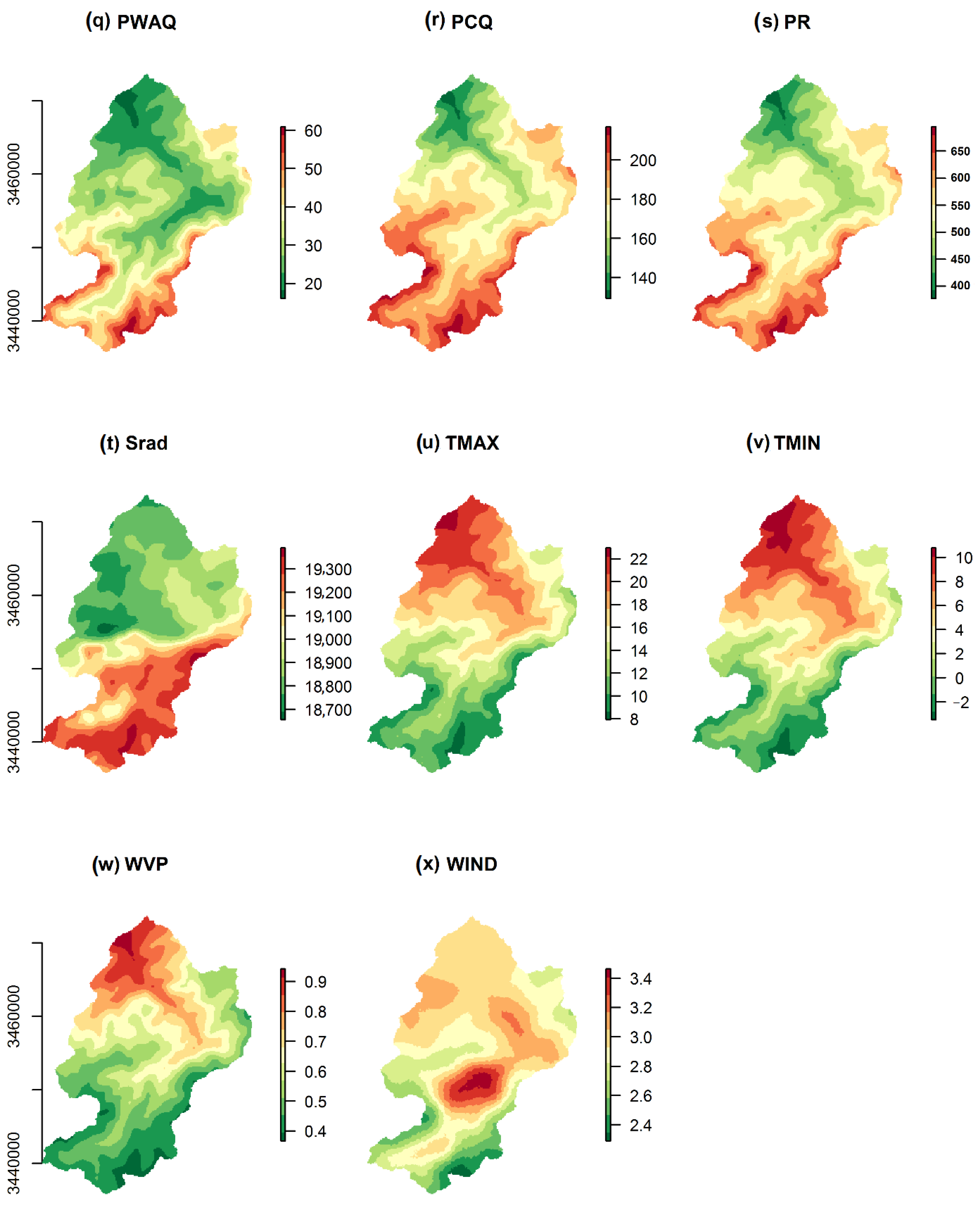
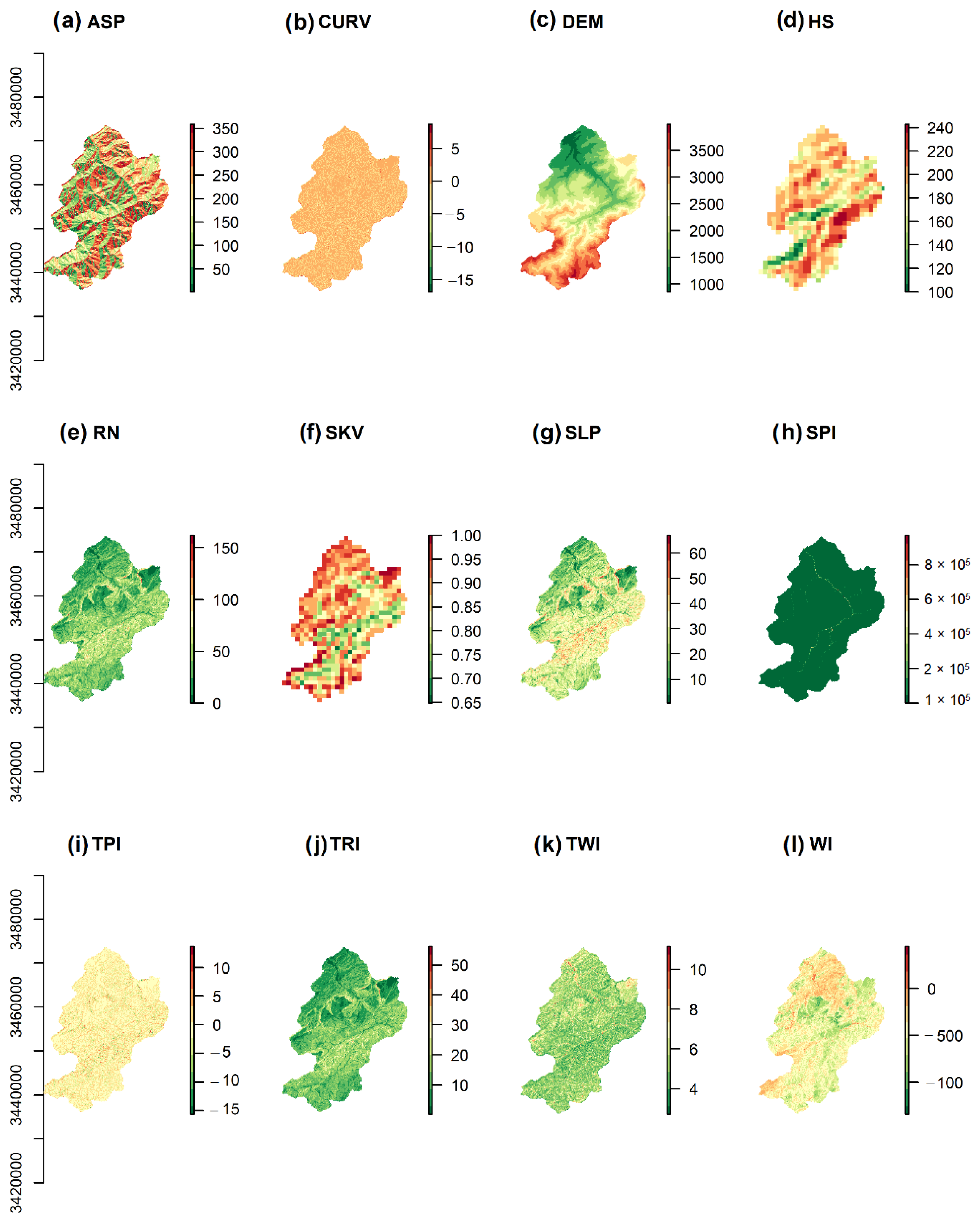
2.3. Predictor Variables for Modeling

There are several drivers and indicators of SOC storage [49,50,51,52]: climate, topography, parent material, organisms (i.e., natural vegetation, land use and management, soil biota, etc.), and soil properties (i.e., soil type, soil aggregation, silt and clay content, clay mineralogy and specific surface area, among others). Climatic conditions, notably temperature and precipitation, affect SOCS on a global and regional scale by influencing both the supply of carbon to the soil and its decomposition dynamics [51]. Topography impacts SOC storage due to its effect on precipitation, water flow and accumulation, and erosive processes. The influence of bedrock on SOCS is related to its impact on soil characteristics, including texture, mineralogy, and therefore fertility, which collectively impact net primary productivity [53]. Vegetation and land use influence SOCS dynamics through the depth distribution of organic carbon, which varies among different plant functional types due to different carbon allocation patterns [54]. As for soil type, texture, and structure, they represent one of the driving factors influencing SOCS [51,55,56]. Indeed, soil structure is enhanced by organic matter by improving physical properties through different organic binders [50]. The interaction between soil mineralogy and SOCS has been the subject of much research, with clay and silt found to influence SOC stabilization, thereby controlling soil carbon sequestration [57].

Data used for this study were obtained from various sources. Chemical and physical property variables were collected from SoilGrids (https://soilgrids.org/ (accessed on 4 May 2022): [58]), while climate predictors were downloaded from WordClim (https://www.worldclim.org/ (accessed on 4 May 2022): [59]). Topographic variables were extracted from a 30 m digital elevation model (DEM) obtained from the ASTER GDEM platform (https://asterweb.jpl.nasa.gov/gdem.asp, accessed on 18 May 2022), while remote sensing predictors were obtained from Landsat 8 images downloaded from the USGS GLOVIS platform (https://glovis.usgs.gov/app, accessed on 18 May 2022). In order to integrate the different variables in the different modeling steps of SOCS, it was necessary to extract the data related to the study watershed. Accordingly, this was performed in an R environment, and the respective variables and predictors are shown in Figure A1, Figure A2, Figure A3 and Figure A4. Soil variables (Figure A1) included BD, cation exchange capacity at neutral pH, carbon density, coarse fragments, clay, silt, nitrogen, and sand contents, each at different depths (0–5 cm, 5–15 cm, 15–30 cm) and soil types. Climate predictors, topographic variables, and remote sensing variables are also presented in Figure A2, Figure A3 and Figure A4, respectively.

2.4. Regression Algorithms

2.4.1. Random Forest (RF)

Developed by Breiman [60], RF is composed of several decision trees, working independently on a view of a problem. The efficiency of RF models strongly depends on the quality of the initial data sample. RF is based on the bagging principle. A dataset is initially split into smaller groups (decision trees), after which a training model is set up for each group. The output of these decision trees is then aggregated to produce the most reliable prediction.

2.4.2. Cubist

Cubist is a development of Quinlan’s [61] M5 model tree. It is structured on the basis of a developed tree, where the linear regression models are located in the terminal leaves. Intermediate linear models are identified at each stage of the tree, and the models are based on the predictors employed in the previous divisions. The linear regression model makes a prediction at the terminal node of the tree while taking into account the prediction of the linear model at the node before it.

2.4.3. Support Vector Machine (SVM)

SVMs were created in the 1990s by the team led by Vapnik [62] and are known for their simplicity and versatility in handling problems. The goal is to classify data using a simple boundary that allows the difference between unique groups of data, called the margin, to be small enough to allow for a better understanding of the data. Support vectors (SVMs), which correspond to the data closest to the boundary, are called large-margin separators.

2.4.4. Gradient Boosting Machine (GBM)

GBM is based on a bagging-like concept, where the boosting process works sequentially in model creation. Initially, a preliminary model is created, which is then evaluated. A weighting is then assigned to each individual based on the performance of the prediction. Its purpose is to give more weight to individuals that were poorly predicted when building the next model. The weights can be adjusted as needed to improve our ability to predict poorly predicted values. To create each new model, this approach determines the weights of individuals using the gradient of the loss function.

2.5. Variable Selection and Cross Validation

Variable selection improves model accuracy by focusing the algorithms on the most relevant predictors. This approach eliminates unnecessary information that can lead to overfitting and, consequently, to erroneous conclusions while reducing computational costs. Another approach that helps prevent model overfitting is the cross-validation of data. It involves splitting the data into training and test subsets and evaluating model performance accordingly. Variable selection techniques include recursive feature elimination (RFE) and forward feature selection (FFS). FFS has demonstrated suitability with a strong interest in spatial variable selection, as highlighted by Meyer et al. [63]. Alternatively, it can be combined with cross-validation to identify the predictors conditioning the maximum performance [63]. In this study, the R package CAST was used to implement FFS with 10 × 10 repeated cross-validation. Variable selection was performed for each learning-response algorithm.

2.6. Modeling, Models Comparison and Validation

The sample set of observations was randomly divided into subsets in an 80:20 split. Accordingly, the first subset (80%) represented the sample data used for model training, while the remaining 20% was used for testing. To better characterize the error distribution of the models, a 10 × 10 repeated cross-validation resampling strategy was used when training the models. The robustness of the models was assessed based on the test data using the mean prediction error (ME), mean absolute prediction error (MAE), root mean squared prediction error (RMSE), and coefficient of determination (R²), whose calculations are given in (3)–(6), respectively.

$$\mathrm{MAE}=\frac{1}{\mathrm{N}}{\displaystyle \sum }_{\mathrm{i}=1}^{\mathrm{N}}\left|\mathsf{\epsilon } \left({\mathrm{S}}_{\mathrm{i}}\right)\right|$$

(3)

$$\mathrm{MAE}=\frac{1}{\mathrm{N}}{\displaystyle \sum }_{\mathrm{i}=1}^{\mathrm{N}}\left|\mathsf{\epsilon } \left({\mathrm{S}}_{\mathrm{i}}\right)\right|$$

(4)

$$\mathrm{RMSE}=\sqrt{\frac{1}{\mathrm{N}}{\displaystyle \sum }_{\mathrm{i}=1}^{\mathrm{N}}\mathsf{\epsilon } {\left({\mathrm{S}}_{\mathrm{i}}\right)}^2}$$

(5)

$${\mathrm{R}}^2={\left(\frac{{{\displaystyle \sum }}_{\mathrm{i}=1}^{\mathrm{N}}\left(\mathrm{z} \left({\mathrm{s}}_{\mathrm{i}}\right)- \overline{\mathrm{z}}\right)\left(\widehat{\mathrm{z} }\left({\mathrm{s}}_{\mathrm{i}}\right)-\overline{\widehat{\mathrm{z} }}\right)}{\sqrt{{{\displaystyle \sum }}_{\mathrm{i}=1}^{\mathrm{N}}{\left(\mathrm{z} \left({\mathrm{s}}_{\mathrm{i}}\right)- \overline{\mathrm{z}}\right)}^2}\sqrt{{{\displaystyle \sum }}_{\mathrm{i}=1}^{\mathrm{N}}{\left(\widehat{\mathrm{z} }\left({\mathrm{s}}_{\mathrm{i}}\right)-\overline{\widehat{\mathrm{z} }}\right)}^2}}\right)}^2$$

(6)

An important advantage over existing approaches to assessing map quality is the evaluation based on the combined effect of several statistical parameters rather than a single index or list of indices [64,65]. Wadoux et al. [65] recommend the combination of commonly used statistics through diagrams, which consists of an integrated approach to evaluating quantitative soil maps through Taylor and solar diagrams. Accordingly, these diagrams were used in this study to evaluate predicted SOCS values.

A soil map can be evaluated based on a comparison between predictions from calibration locations and actual data. Yet, the resulting internal accuracy frequently overestimates the actual accuracy [66]. Thus, it is best to compare predictions to independent data that were not used in the modeling. External accuracy or test accuracy are terms used to describe this. In this study, the external accuracy of the maps was determined by estimating them using randomly distributed data, thus maintaining the characteristics of probability sampling [67].

To investigate model validity domains and map uncertainty, the infinitesimal jackknife method [68,69,70] was used to estimate the variability of predictions made by RF for the SOCS at 0–30 cm depth.

3. Results

3.1. Variable Selection and Variable Importance

Table 2. Models and predictors used with forward feature selection.

Model	Used Predictors with FFS	Abbreviation
Cubist	All predictors	Cub
GBM	All predictors	GBM
SVM	All predictors	SVM
RF	All predictors	rf_all
RF	Bioclimatic variables	rf_b
RF	SoilGrids soil variables	rf_s
RF	Remote sensing variables	rf_rs
RF	Topographical variables	rf_t
RF	Bioclimatic and SoilGrids soil variables	rf_bs
RF	Bioclimatic and Remote sensing variables	rf_brs
RF	Bioclimatic and topographic variables	rf_bt
RF	SoilGrids soil variables and topographic variables	rf_st
RF	Remote sensing and topographic variables	rf_rst
RF	SoilGrids soil variables and remote sensing variables	rf_srs

presents the 14 models trained and the predictors used with the direct feature selection algorithm. LU/LC was used as a predictor for all trained models. The best-fit hyperparameters of the models are presented in Table S1. For each of the 11 RF-trained models, LU/LC was found to be the most influential variable with an importance score of 100% (Figure 2), demonstrating its contribution to controlling the spatial distribution of SOCS in the Ourika watershed. On the other hand, the most important variables for Cubist and GBM were elevation (DEM) and cation exchange capacity (CEC.5.15) respectively, both with variable scores of 100%.

Isothermality (ISOTH), mean temperature of the coldest quarter (TCQ), and mean temperature of the wettest quarter (TWEQ) were the most important variables for RF trained with only bioclimatic variables (rf_b), presenting relative importance scores of 32.17%, 24.10%, and 23.53%, respectively. As for the RF trained with only the soil variables (rf_s), the clay fraction (0–5 cm: CL.0.5) was the most important variable, with an importance score of 50.30%. The modified nonlinear vegetation index (MNLVI) was the most influential variable for RF trained only with remote sensing variables (rf_rs), presenting an importance score of 7.33%, while for RF coupled with topographic variables (rf_t), LU/LC was essentially the only predictor. The analysis pertaining to the combination of bioclimatic and soil variables (rf_bs) highlighted TWEQ and DR as the most important variables, with relative importance scores of 57.08% and 6.71%, respectively, while the combination of bioclimatic and remote sensing variables (rf_brs) indicated TWEQ and MNLVI as the most influential, with relative importance scores of 26.94% and 8.52%, respectively. For the combination of bioclimatic and topographical variables (rf_bt), the most important variables were TWEQ, DEM, mean diurnal range (DR), and temperature annual range (TAR), with relative importance scores of 24.57%, 17.33%, 14.46%, and 12.37%, respectively. Based on the combination of soil and topographical variables (rf_st), the most influential variables were WI, CEC.5.15, Nitrogen (15–30 cm: N.15.30), and hillshade (HS), presenting relative importance scores of 26.72%, 25.86%, 23.11%, and 20.57%, respectively. As for the combination of remote sensing and topographical variables (rf_rst), the most relevant variables were DEM, land surface temperature from LANDSAT 8 Band 11 (LST11), HS, and renormalized difference vegetation index (RDVI), with relative importance scores of 34.61%, 25.15%, 20.70%, and 20.46%, respectively. The most influential variables for the combination of soil and remote sensing variables (rf_srs) were CL.0.5, RDVI, and CEC.5.15, presenting importance scores of 16.57%, 14.56%, and 12.22%, respectively.

3.2. Model Evaluation Using Cross Validation

Figure 3 shows the distribution of error metrics for prediction after 10 × 10 cross-validation for the RF, Cubist, SVM, and GBM algorithms on the training set. RF and Cubist were demonstrably the most accurate models. Indeed, they presented comparatively low MAE and RMSE values while being the best-fitting models, with RF being the better of the two (MAE = 10.77 t/ha, RMSE = 13.37 t/ha, R² = 0.72). Figure 4 shows the results of the absolute error distribution for RF and highlights the predictive ability of the model. However, there is a notable loss of accuracy for areas characterized by high SOCS content. These represent areas of the watershed where the land cover is dominated by dense and moderately dense forests, which are generally characterized by high variability. In contrast to RF, SVM exhibited the lowest predictive power (MAE = 13.53 t/ha, RMSE = 17.95 t/ha, R² = 0.51).

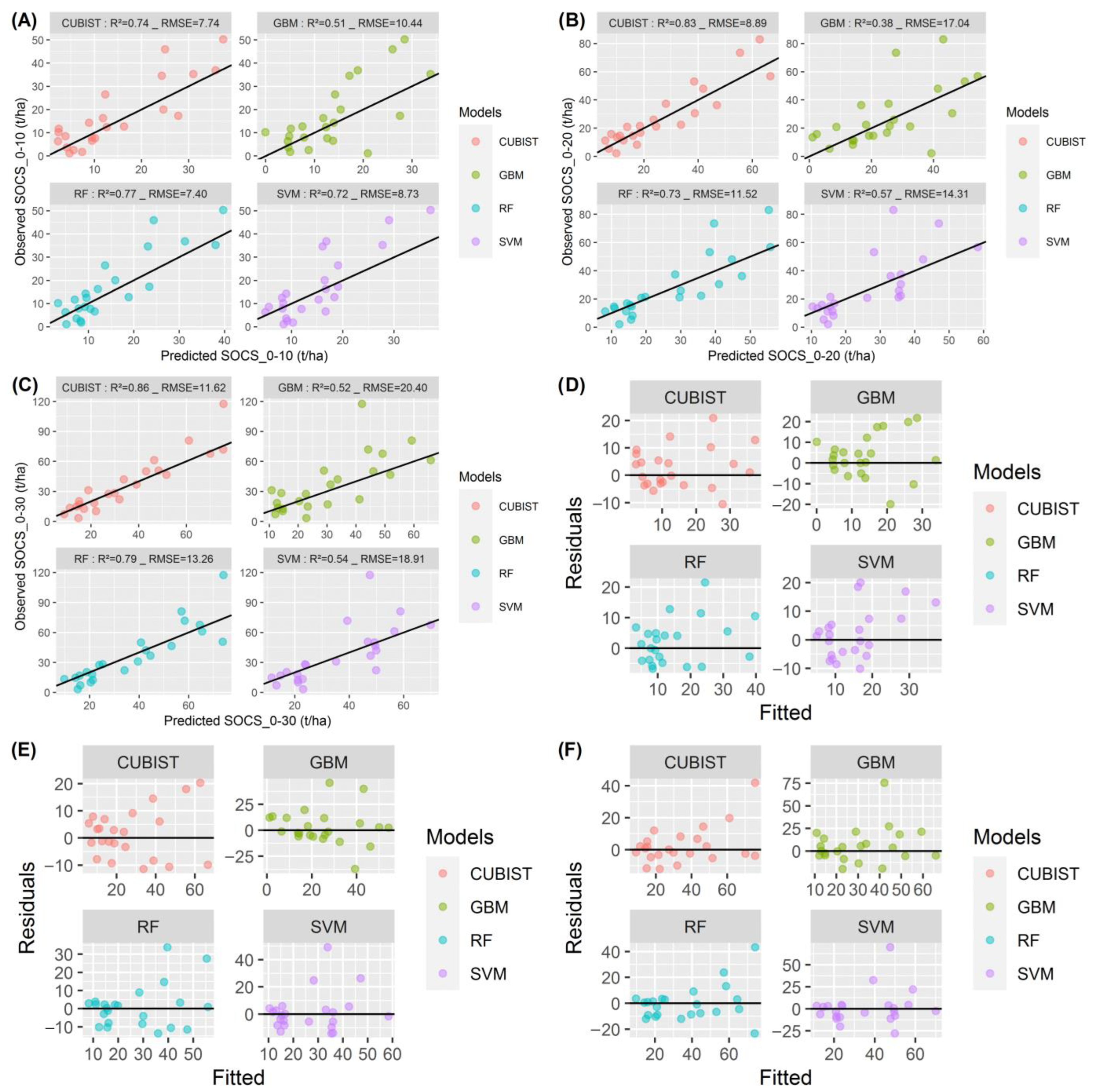
3.3. Model Evaluation and Comparison Based on the Testing Data

Figure 5 shows the R² and RMSE values for the prediction of the different models based on the test data. For SOC prediction at a depth of 0–10 cm, Cubist was the best performing model with RMSE of 0.46% (R² = 0.88). The following models in terms of performance were the RF, SVM, and GBM, with RMSE values of 0.59%, 0.66%, and 1.07%, respectively, and R² values of 0.79, 0.75, and 0.32, respectively. At a depth of 0–20 cm, RF was the most accurate model for predicting SOC, with an RMSE of 0.9% (R² = 0.80). This was followed by Cubist, SVM, and GBM with RMSEs of 0.93%, 1.25%, and 1.48%, respectively, and R² values of 0.79, 0.62, and 0.48, respectively. At a depth of 0–30 cm, for SOC prediction, RF and Cubist showed the smallest RMSE at 1.2%, followed by SVM and GBM with RMSE values of 1.61% and 2.05%, respectively. Their respective R² values were 0.79, 0.77, 0.59, and 0.36 for RF, Cubist, SVM, and GBM. The results revealed an increase in prediction errors with depth, ranging from 0.46% to 1.2%, 0.59% to 1.2%, 0.66% to 1.61%, and 1.07% to 2.05% for Cubist, RF, SVM, and GBM, respectively. Thus, for SOC prediction, RF and Cubist were shown to be the best performing models.

A strong relationship between observed and predicted SOC values is evidenced (Figure S1), while no apparent relationship is observed between residuals and fitted values, especially for the RF and Cubist models. None of the models showed the ability to predict BD with acceptable accuracy (R² < 0.40; RMSE > 0.2 g/cm³). A weak relationship was obtained between observed and predicted BD, and an apparent relationship was noted between residuals and fits (Figure S2), which highlights an overall poor performance of the model in predicting BD.

RF was the most accurate model (R² = 0.77; RMSE = 7.40 t/ha) for predicting SOCS at a depth of 0–10 cm, while Cubist had the greatest predictive power at both 0–20 cm (R² = 0.83, RMSE = 8.89 t/ha) and 0–30 cm (R² = 0.86, RMSE = 11.62 t/ha). Effectively, the two models performed best in predicting SOCS. In contrast, the GBM model demonstrated the lowest accuracy in predicting SOCS for all depth classes. Figure 6 shows the relationship between observed and predicted SOCS, as well as the relationship between residuals and fitted values. While there was a strong relationship between the observed and predicted SOCS, no discernable relationship was observed between the residuals and the fitted values, especially for the RF and Cubist models.

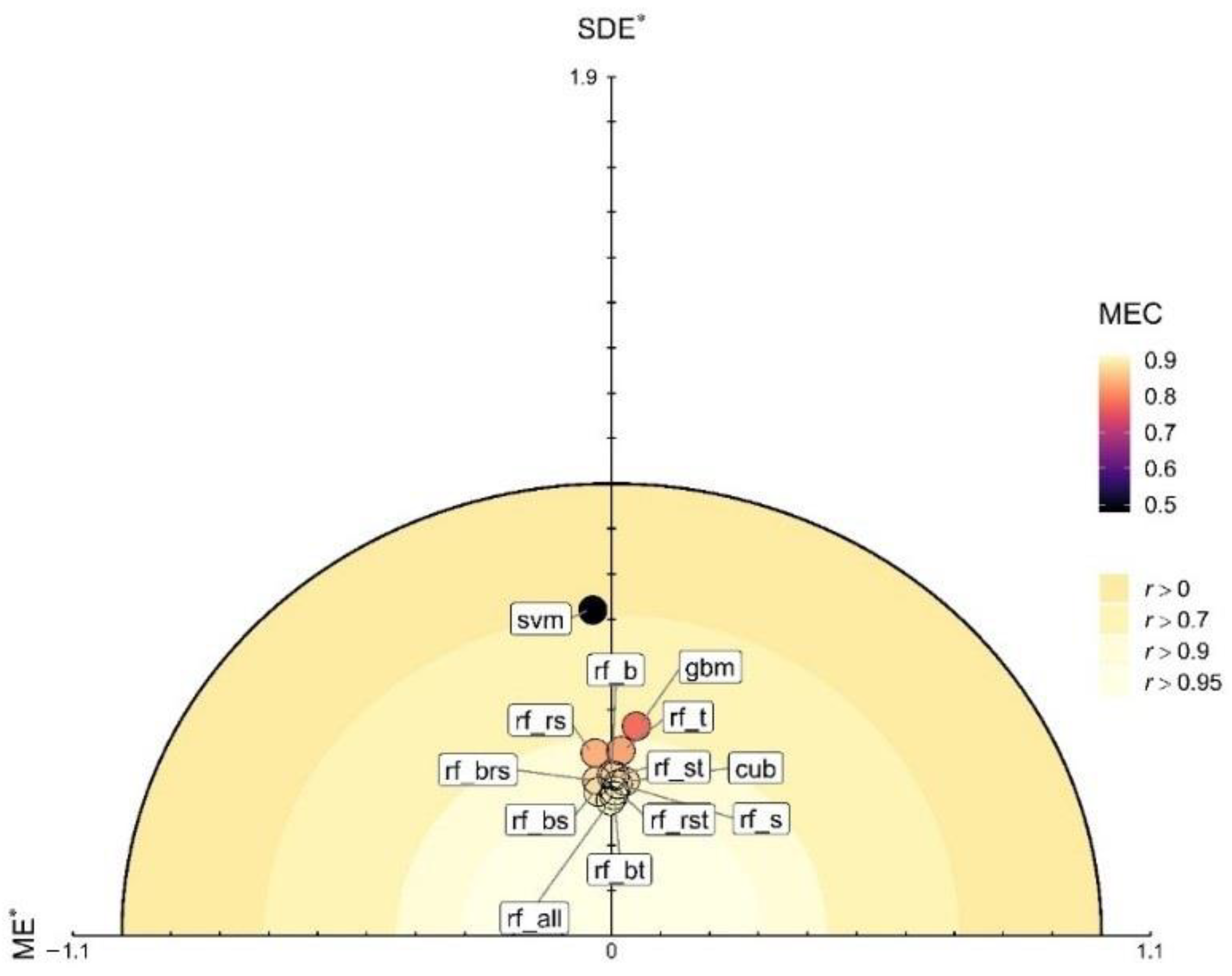
3.4. Contribution of Explanatory Factors and Integrated Evaluation of the Predictions

The metrics for assessing the quality of the predictions are presented in

Table 3. Statistics of quality for the predicted and observed SOCS_0-30.

Models	ME	MAE	RMSE	R2
rf_all	−0.07	5.33	7.58	0.92
cub	0.7	6.43	8.68	0.89
svm	−0.98	13.39	18.29	0.51
gbm	1.29	7.92	11.82	0.79
rf_b	−0.01	6.39	9.01	0.89
rf_s	0.33	6.16	8.49	0.9
rf_rs	−0.86	7.04	10.29	0.85
rf_t	0.49	7.64	10.38	0.84
rf_bs	−0.7	6.03	8.09	0.91
rf_brs	−0.77	5.78	8.74	0.89
rf_bt	0.13	5.59	7.87	0.92
rf_st	0.17	6.02	8.97	0.9
rf_rst	0.18	5.65	8.12	0.92
rf_srs	−0.57	5.78	8.05	0.91

. The results of the ME analysis showed that all predictions had either a positive or negative bias. Based on the observed values, the least biased models were rf_b and rf_all, with ME values of −0.01 and −0.07, respectively, while the most biased models were GBM and SVM, with ME values of 1.29 and −0.98, respectively.

Despite the inclusion of both WorldClim bioclimate and SoilGrids variables derived from their associated modeling, this study has shown their potential to improve the accuracy and performance of the models. Indeed, the RF models using only topographic (rf_t) and remote sensing (rf_rs) predictors exhibited the lowest accuracies, with RMSE values of 10.38 t/ha (R² = 0.84) and 10.29 t/ha (R² = 0.85), respectively. In contrast, combining the bioclimatic and SoilGrids variables with the other selected predictors resulted in higher accuracies, with the best-performing model being the RF coupled with bioclimatic and topographic variables (rf_bt), which resulted in the lowest RMSE value of 7.87 t/ha (R² = 0.92). Similar improvements in model accuracy were observed when combining bioclimatic and remote sensing variables (rf_brs), as indicated by an RMSE of 8.74 t/ha (R² = 0.89). Consistent with observations using bioclimatic variables, SoilGrids predictors were found to improve model accuracy. Indeed, RF coupled with the combination of SoilGrids variables and topographic variables (rf_st), and remote sensing variables (rf_srs) resulted in generally low RMSE values of 8.97 t/ha (R² = 0.92) and 8.05 t/ha (R² = 0.90), respectively.

The results of the prediction accuracy assessment indicated that the most accurate models were rf_all (MAE = 5.33, RMSE = 7.58, R² = 0.92), rf_bt (MAE = 5.59, RMSE = 7.87, R² = 0.92), rf_srs (MAE = 5.78, RMSE = 8.05, R² = 0.92), and rf_rst (MAE = 5.65, RMSE = 8.12, R² = 0.91).

Evaluation of the different environmental covariates indicated that soil properties extracted from SoilsGrid (SGV) predicted SOCS with the lowest errors (RMSE = 8.49), followed by bioclimatic variables (BCV) (RMSE = 9.01). In contrast, prediction errors were higher for remote sensing variables (RSV) and topographic variables (TOV), which presented RMSE values of 10.29 and 10.38, respectively. In addition, the pairwise combination of covariates showed that BCV + TOV had the best predictive performance (RMSE = 7.84) while SGV + TOV (RMSE = 8.97) represented the weakest combination. Accordingly, the best covariate combinations that improved predictive performance were BCV + TOV and SGV + RSV (RMSE = 8.05).

The 14 predictions considered are presented on the Taylor diagram (Figure 7) and the Solar diagram (Figure 8). The points closest to the reference point represent the least biased predictions. Both diagrams show that the least biased predictions are rf_all, rf_bt, rf_srs, and rf_bs, while the most biased models are svm, gbm, rf_t, and rf_rs.

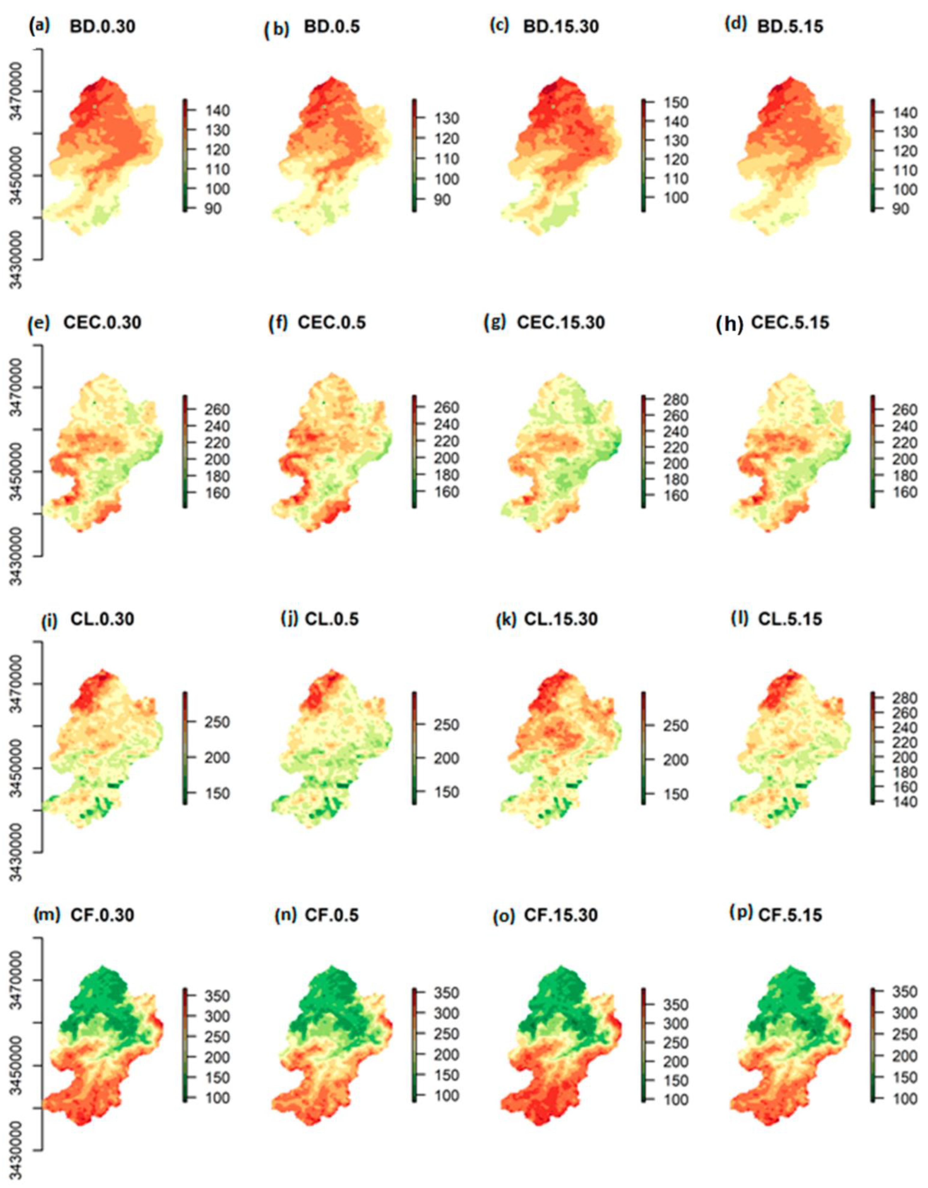
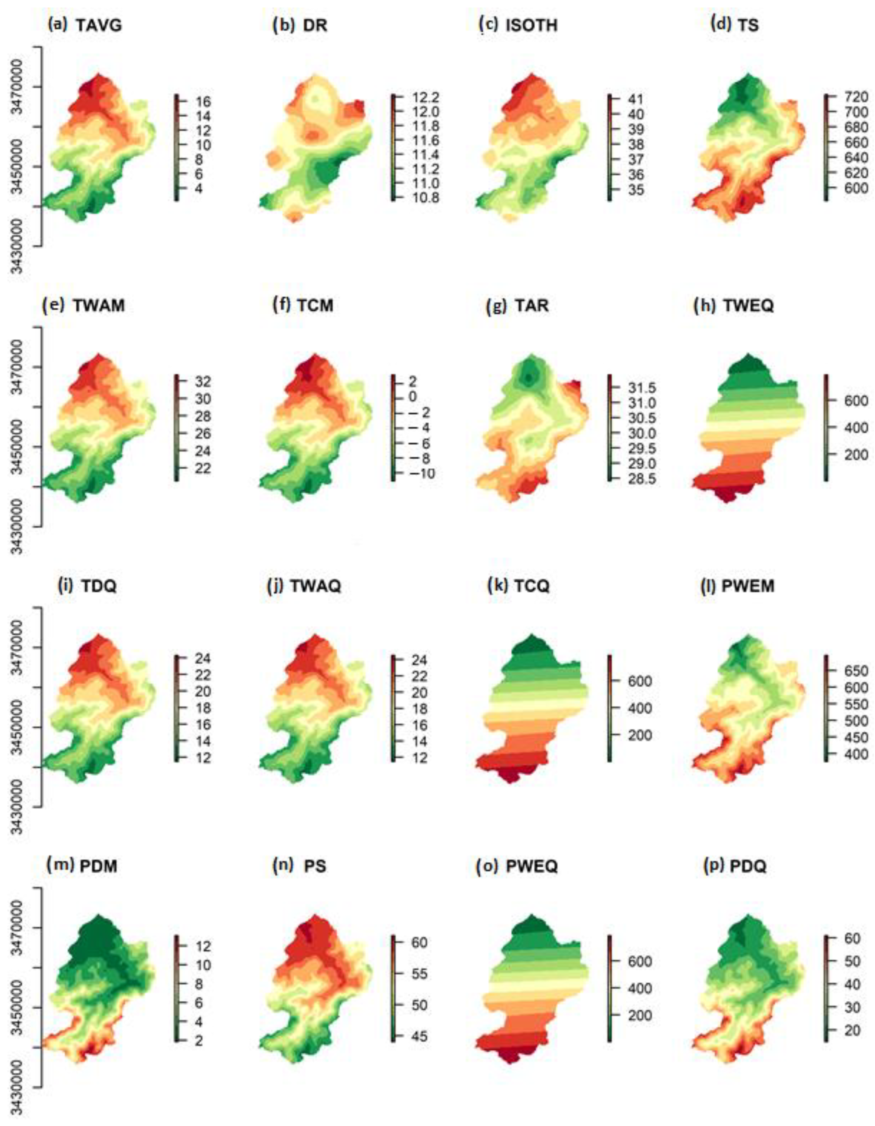
3.5. Spatial Prediction of SOC and SOCS

Figure 9 and Figure 10 show the SOC and SOCS predicted by the RF and Cubist models. The highest SOC and SOCS contents were predicted for the central and northwestern sections of the watershed. These represent the generally low-lying areas of the watershed where elevations rarely exceed 1500 m. In addition, this region features areas of the watershed with decent forest cover that is characterized by a predominance of Barbary thuja, holm oak, and juniper. Conversely, the lowest predicted values were observed in the southern portion of the watershed, where the elevation is highest, reaching up to 3500 m, and where the characteristic land cover is a dominance of upland xerophytes and bare soil. With the exception of SOC predictions at the 0–30 cm depth where RF appeared to predict higher values than Cubist, there was a strong similarity in SOC and SOCS predictions at all depths by both models (Figure 10).

Interestingly, a comparison between these results and the results of the direct calculation of SOCS (Figure A5) from the predicted SOC content and BD highlights a tendency for the latter approach to underestimate SOCS throughout the watershed. This is particularly notable for the estimate of SOCS in the top 20 cm of soil, which shows that almost the entire watershed is characterized by low to very low SOCS.

The standard error of the SOCS prediction ranged from 3.1 to 15.4 t/ha, with a mean value of 3.4 ± 0.8 t/ha, while the ratio of MSE to mean SOCS prediction ranged from 0.03 to 0.92, with a mean value of 0.17 ± 0.07 (

Table 4. Analysis of mean predicted SOCS (0–30) and mean standard error (MSE) by LU/LC type.

LU/LC	Mean Predicted SOCS (t/ha)	MSE (t/ha)	MSE/Mean Predicted SOCS Ratio
Thorny upland xerophytes	16.62	3.22	0.19
Open holm oak stands	18.05	3.31	0.18
Dense holm oak stands	57.27	3.93	0.07
Moderately dense holm oak stands	50.23	3.52	0.07
Agriculture	41.19	4.37	0.11
Open juniper stands	20.26	3.31	0.16
Moderately dense juniper stands	47.05	4.22	0.09
Reforestation	25.80	3.38	0.13
Open Barbary thuja stands	25.04	3.52	0.14
Dense Barbary thuja stands	67.17	3.82	0.06
Moderately dense Barbary thuja stands	54.42	3.91	0.07

; Figure 11). The highest ratios of MSE to mean SOCS prediction were observed in areas with limited vegetation cover, such as upland thorny xerophytes, open forests, and croplands. These areas are also associated with low SOCS variability and thus low SOCS. In contrast, the lowest ratios were observed in dense and moderately dense forests, which have high canopy cover, high SOS content, and high SOCS variability. The models’ skill in predicting SOCS was high in dense and moderately dense forests, which could be ascribed to their high SOC content and high SOCS variability. Conversely, model accuracy was low in areas with sparse vegetation cover, low SOCS content, and low SOCS variability. The difficulty in accurately predicting SOCS in areas with low vegetation cover indicates a possible limitation of the models. Nevertheless, these results highlight the importance of vegetation cover as a parameter in accurately predicting SOCS in the watershed.

4. Discussion

Previous studies undertaken in Morocco have reported generally low SOM content and continuous decline in most soils due to factors such as intensive land use, making it imperative to conduct studies to assess the evolution of SOC and SOCS in soils, as this could be essential in the strategic management of vulnerable areas. In this study, an ML approach using RF, Cubist, SVM, and GBM algorithms was adopted for the prediction and mapping of SOCS for the Ourika watershed. Among the factors explored and variables used for modeling, LU/LC was found to be the most influential predictor of SOC and SOCS distribution. These findings are consistent with the observations of Wiesmeier et al. [71] who reported land use and associated soil types being the most critical variables controlling SOC distribution. LU/LC has been reported as a major factor influencing SOC concentration [72,73,74], and this is attributed to the impact of land use changes and land cover types on SOC accumulation and turnover.

The comparison of the different groups of environmental covariates showed that soil properties extracted from SoilsGrids and bioclimatic variables were the most relevant factors for SOCS in the Ourika watershed. Correspondingly, the combination of bioclimatic and topographic variables as well as soil properties and remote sensing variables resulted in improved prediction performance. Accordingly, this observation is supported by the work of Adhikari et al. [17] and John et al. [75] who highlighted in their respective studies in India and Nigeria the usefulness of a combination of environmental and soil variables in explaining SOC distribution and thus their influential role as predictors. Although the bioclimatic variables from WorldClim and the soil variables from SoilGrids were derived from their respective models, their incorporation as predictive variables improved the model performance in this study. Notwithstanding, the simple use of topographic and remotely sensed variables as predictors resulted in relatively high model accuracy for SOCS prediction, which is consistent with the study conducted by Zhou et al. [76] who noted that a combination of only satellite image-derived predictors and DEM-derived predictors resulted in the highest predictive accuracy for SOC in Central Europe.

Overall, RF and Cubist were the most accurate models for predicting SOC and SOCS in the watershed. Comparable results were reported by John et al. [75], where RF and Cubist exhibited the best prediction accuracy. Notably, both models have been shown to capture nonlinear relationships between predictive controllers and SOC and SOCS, as was the case in this study, producing high predictive accuracy comparable to methods such as regression kriging, as noted by Mishra et al. [77]. The predictive superiority of RF, particularly, in SOC mapping is well recognized in the literature [37,40,78,79,80,81]. However, this is not always the case, as shown by Were et al. [74] who reported that SVM outperformed RF in mapping SOCS in Kenya. Similarly, Zhou et al. [76] reported that the boosted regression tree model (BRT) was superior to RF in predicting SOC using satellite imagery and topographic variables. These observations reflect the fundamentally discordant nature of prediction results using ML models, highlighting the importance of focusing on the quality of the prediction data to calibrate the models rather than attempting to find an outright best prediction model.

As noted in this study, the central and northwestern sections of the watershed were predicted to have the highest contents of SOC and SOCS, while almost the entire lower half of the watershed was poor in both. These SOC-rich regions represent areas of comparatively favorable conditions, where the generally low-elevation areas of the watershed feature relatively rich vegetation cover consisting of forest species such as holm oak (Quercus rotundifolia), juniper (Juniperus sp.), Barbary thuja (Tetraclinis articulata), among others. This helps provide potentially favorable conditions for SOCS accumulation and low SOC turnover. High SOCS in forested lands is attributed to minimal soil disturbance and a slow rate of SOC decomposition, resulting in higher SOC accumulation [82]. In addition, natural forests are generally associated with low BD through minimal disturbance, which promotes carbon accumulation and storage [83,84]. In contrast, high-elevation sections characteristic of the southern half of the watershed were predicted to contain the lowest SOCS, which is inconsistent with the general observation of high SOCS content at higher elevations. High SOCS at higher elevations is related to factors such as low temperatures leading to lower SOM decomposition rates; high precipitation leading to rich vegetation cover that promotes organic matter accumulation; and limited disturbance from anthropogenic activities due to inaccessibility [85,86]. However, in the watershed selected for this study, these areas were characterized by limited vegetation with a dominance of thorny xerophytes that are poor in litter, and therefore would account for the predicted low SOCS.

Morocco is characterized by a relatively low SOCS due to a combination of anthropogenic factors and climatic conditions that accelerate soil degradation [87]. This is true for the watershed we studied, which is located in an area conducive to erosion phenomena due to geomorphological and climatic conditions as well as anthropogenic factors [88]. Inappropriate land use, often manifested by the clearing of forest cover for agriculture, accentuates these phenomena, which can lead to the depletion of organic matter and, consequently, of SOC. This results in a loss of soil fertility and a decrease in the soil’s capacity to sequester carbon [41]. The results of this study showed the importance of addressing and monitoring the evolution of SOC in the different LU/LC characterizing the area. Notably, the models in the study showed promising results in accurately predicting SOCS, suggesting that this approach could be useful in promoting sustainable land management in the watershed as well as in other vulnerable regions of the country. The modeling approach using readily available data shows the potential of the approach, and would help policy makers and land managers to make informed decisions on sustainable management of watershed resources, mainly those affecting soils.

Overall, ML provides an intriguing tool for soil studies. Assessing SOCS and their evolution in the region ensures that adequate and appropriate measures are applied to ensure the continued role of soil in carbon sequestration. Nevertheless, these methods have inherent limitations and complexities. As noted in the literature, factors such as predictor selection for modeling have the potential to influence model performance and complexity. For instance, Song et al. [89] and Li et al. [90] noted that soil properties provide better predictors for SOC prediction in small homogeneous areas, while environmental attributes are more influential at a larger and more complex scale. Thus, a comprehensive study of all the steps involved in modeling, including the judicious selection of the most appropriate model inputs, is essential to mitigate these issues.

5. Conclusions

This study aimed to explore the applicability and implication of the ML approach in the prediction and mapping of SOC(S) at the watershed scale in the High Atlas region of Morocco. The type and quality of data were highlighted as vital in the modeling process, where, in particular, combinations of bioclimatic and topographic variables as well as soil properties and remote sensing variables, were shown to greatly improve model performance. RF and Cubist demonstrated the best performance of the four selected models in predicting SOCS. While RF in particular has been very successful in many regions and under several environmental conditions, confirming its reliability and its predictive superiority is not always the case, as some studies show. On this basis, no single predictive model can be considered definitively the best in all circumstances. It is therefore meaningful to focus the approach on finding the most appropriate experimental data that will better calibrate the predictive models for each specific case study rather than searching for the absolute best model. The widely recognized role of LU/LC in impacting SOC dynamics was confirmed in this study, as it was the factor that most influenced the prediction of ML models. The highest SOC levels were predicted in areas where dense and moderately dense forest cover was a dominant feature, while the lowest were predicted in ecosystems characterized by a predominance of bare soil and upland thorny xerophytes that generally reflect forest cover degradation. These results support the need to protect and conserve vegetation cover, particularly natural forests in the region, so that they can fulfill their role in promoting SOC sequestration. The information, including maps resulting from the SOCS prediction, can be used to help identify areas requiring immediate attention for activities (e.g., reforestation) to improve conditions that facilitate SOC storage.

References

1. Lal, R. Soil Carbon Sequestration to Mitigate Climate Change. Geoderma 2004, 123, 1–22. [Google Scholar] [CrossRef]
2. Aticho, A. Evaluating organic carbon storage capacity of forest soil. Case study in Kafa Zone BitaDistrict, Southwestern Ethiopia. Am. Eurasian J. Agric. Environ. Sci. 2013, 13, 95–100. [Google Scholar]
3. Stockmann, U.; Adams, M.A.; Crawford, J.W.; Field, D.J.; Henakaarchchi, N.; Jenkins, M.; Minasny, B.; McBratney, A.B.; de Courcelles, V.d.R.; Singh, K.; et al. The knowns, known unknownsand unknowns of sequestration of soil organic carbon. Agric. Ecos. Environ. 2013, 164, 80–99. [Google Scholar] [CrossRef]
4. Jandl, R.; Rodeghiero, M.; Martinez, C.; Cotrufo, M.F.; Bampa, F.; Wesemael, B.V.; Harrison, R.B.; Guerrini, I.A.; Richter, D.D.; Rustad, L.; et al. Currentstatus, uncertainty and future needs in soil organiccarbon monitoring. Sci. Total Environ. 2014, 468, 376–383. [Google Scholar] [CrossRef]
5. Shelukindo, H.B.; Semu, E.; Msanya, B.; Singh, B.R.; Munishi, P. Soil organic carbon stocks in the dominant soils of the Miombo woodland ecosystem of Kitonga Forest Reserve, Iringa, Tanzania. Int. J. Agric. Policy Res. 2014, 2, 167–177. [Google Scholar]
6. Greve, M.H.; Greve, M.B.; Bou Kheir, R.; Bøcher, P.K.; Larsen, R.; McCloy, K. Comparing Decision Tree Modeling and Indicator Kriging for Mapping the Extent of Organic Soils in Denmark; Digital Soil Mapping Bridging Research, Environmental Application, and Operation; Boettinger, J.L., Howell, D.W., Moore, A.C., Hartemink, A.E., Kienast-Brown, S., Eds.; Springer: Dordrecht, The Netherlands; Heidelberg, Germany; London, UK; New York, NY, USA, 2009. [Google Scholar]
7. Luo, Z.; Wang, E.; Sun, O.J. Soil carbon change and its responses to agricultural practices in Australian agro-ecosystems: A review and synthesis. Geoderma 2010, 155, 211–223. [Google Scholar] [CrossRef]
8. Elbasiouny, H.; Abowaly, M.; Abu Alkheir, A.; Gad, A. Spatial variation of soil carbon and nitrogen pools by using ordinary Kriging method in an area of north Nile Delta, Egypt. Catena 2014, 113, 70–78. [Google Scholar] [CrossRef]
9. Lal, R. Forest Soils and Carbon Sequestration. For. Ecol. Manag. 2005, 220, 242–258. [Google Scholar] [CrossRef]
10. Batjes, N. Total Carbon and Nitrogen in the Soils of the World. Eur. J. Soil. Sci. 1996, 47, 151–163. [Google Scholar] [CrossRef]
11. Guo, P.T.; Li, M.F.; Luo, W.; Tang, Q.F.; Liu, Z.W.; Lin, Z.M. Digital mapping of soil organic matter for rubber plantation at regional scale: An application of random forest plus residuals kriging approach. Geoderma 2015, 237, 49–59. [Google Scholar] [CrossRef]
12. Bian, Z.; Guo, X.; Wang, S.; Zhuang, Q.; Jin, X.; Wang, Q.; Jia, S. Applying statistical methods to map soil organic carbon of agricultural lands in northeastern coastal areas of China. Arch. Agron. Soil. Sci. 2019, 66, 532–544. [Google Scholar] [CrossRef]
13. Lefèvre, C.; Fatma, R.; Viridiana, A.; Liesl, W. What is SOC? In Soil Organic Carbon the Hidden Potential; Liesl, W., Ed.; FAO: Rome, Italy, 2017; pp. 1–9. [Google Scholar]
14. Shi, M.J.; Yang, Z.L.; Lawrence, D.M.; Dickinson, R.E.; Subin, Z.M. Spin-up processes in the Community Land Model version 4 with explicit carbon and nitrogen components. Ecol. Modell. 2013, 263, 308–325. [Google Scholar] [CrossRef]
15. De Lannoy, G.J.M.; Koster, R.D.; Reichle, R.H.; Mahanama, S.P.P.; Liu, Q. An updated treatment of soil texture and associated hydraulic properties in a global land modeling system. J. Adv. Model. Earth Syst. 2014, 6, 957–979. [Google Scholar] [CrossRef]
16. Li, X.; McCarty, G.W.; Du, L.; Lee, S. Use of Topographic Models for Mapping Soil Properties and Processes. Soil. Syst. 2020, 4, 32. [Google Scholar] [CrossRef]
17. Adhikari, K.; Hartemink, A.E.; Minasny, B.; Kheir, R.B.; Greve, M.B.; Greve, M.H. Digital mapping of soil organic carbon contents and stocks in Denmark. PLoS ONE 2014, 9, e105519. [Google Scholar] [CrossRef]
18. Fang, H.; Cheng, S.; Yu, G.; Zheng, J.; Zhang, P.; Xu, M.; Li, Y.; Yang, X. Responses of CO2 efflux from an alpine meadow soil on the Qinghai Tibetan Plateau to multi-form and low-level N addition. Plant Soil 2012, 351, 177–190. [Google Scholar] [CrossRef]
19. Viscarra Rossel, R.A.; Walvoort, D.J.J.; McBratney, A.B.; Janik, L.J.; Skjemstad, J.O. Visible, near infrared, mid infrared or combined diffuse reflectance spectroscopy for simultaneous assessment of various soil properties. Geoderma 2006, 131, 59–75. [Google Scholar] [CrossRef]
20. Miltz, J.; Don, A. Optimising Sample Preparation and near Infrared Spectra Measurements of Soil Samples to Calibrate Organic Carbon and Total Nitrogen Content. J. Near Infrared Spectrosc. 2012, 20, 695–706. [Google Scholar] [CrossRef]
21. Walkley, A.J.; Black, I.A. Estimation of soil organic carbon by the chromic acid titration method. Soil. Sci. 1934, 37, 29–38. [Google Scholar] [CrossRef]
22. Mebius, L.J. A Rapid Method for the Determination of Organic Carbon in Soil. Anal. Chim. Acta 1960, 22, 120–124. [Google Scholar] [CrossRef]
23. Nelson, D.W.; Sommers, L.E. Total carbon, organic carbon, and organic matter. In Methods of Soil Analysis. Part 3; Sparks, D.L., Page, A.L., Helmke, P.A., Loeppert, R.H., Eds.; SSSA Book Series: Madison, WI, USA, 1996; pp. 961–1010. [Google Scholar]
24. McBratney, A.B.; Mendonça Santos, M.L.; Minasny, B. On digital soil mapping. Geoderma 2003, 117, 3–52. [Google Scholar] [CrossRef]
25. Taghizadeh-Mehrjardi, R.; Nabiollahi, K.; Kerry, R. Digital mapping of soil organic carbon at multiple depths using different data mining techniques in Baneh region, Iran. Geoderma 2016, 266, 98–110. [Google Scholar] [CrossRef]
26. Tajik, S.; Ayoubi, S.; Shirani, H.; Zeraatpisheh, M. Digital mapping of soil invertebrates using environmental attributes in a deciduous forest ecosystem. Geoderma 2019, 353, 252–263. [Google Scholar] [CrossRef]
27. Goydaragh, M.G.; Taghizadeh-Mehrjardi, R.; Jafarzadeh, A.A.; Triantafilis, J.; Lado, M. Using environmental variables and Fourier Transform Infrared Spectroscopy to predict soil organic carbon. Catena 2021, 202, 105280. [Google Scholar] [CrossRef]
28. Minasny, B.; McBratney, A.B. Spatial prediction of soil properties using EBLUP with Matern covariance function. Geoderma 2007, 140, 324–336. [Google Scholar] [CrossRef]
29. Maynard, J.J.; Dahlgren, R.A.; O’Geen, A.T. Soil carbon cycling and sequestration in a seasonally saturated wetland receiving agricultural runoff. Biogeosciences 2011, 8, 3391–3406. [Google Scholar] [CrossRef]
30. Mondal, A.; Khare, D.; Kundu, S.; Mondal, S.; Mukherjee, S.; Mukhopadhyay, A. Spatial soil organic carbon (SOC) prediction by regression kriging using remote sensing data. Egypt. J. Remote Sens. Space Sci. 2017, 20, 61–70. [Google Scholar] [CrossRef]
31. Zhang, S.; Huang, Y.; Shen, C.; Ye, H.; Du, Y. Spatial prediction of soil organic matter using terrain indices and categorical variables as auxiliary information. Geoderma 2012, 171, 35–43. [Google Scholar] [CrossRef]
32. Veronesi, F.; Schillaci, C. Comparison between geostatistical and machine learning models as predictors of topsoil organic carbon with a focus on local uncertainty estimation. Ecol. Indic. 2019, 101, 1032–1044. [Google Scholar] [CrossRef]
33. Siewert, M.B. High-resolution digital mapping of soil organic carbon in permafrost terrain using machine learning: A case study in a sub-Arctic peatland environment. Biogeosciences 2018, 15, 1663–1682. [Google Scholar] [CrossRef]
34. Pouladi, N.; Møller, A.B.; Tabatabai, S.; Greve, M.H. Mapping soil organic matter contents at field level with Cubist, random forest and kriging. Geoderma 2019, 342, 85–92. [Google Scholar] [CrossRef]
35. Lamichhane, S.; Kumar, L.; Wilson, B. Digital soil mapping algorithms and covariates for soil organic carbon mapping and their implications: A review. Geoderma 2019, 352, 395–413. [Google Scholar] [CrossRef]
36. Zeraatpisheh, M.; Jafari, A.; Bodaghabadi, M.B.; Ayoubi, S.; Taghizadeh-Mehrjardi, R.; Toomanian, N.; Kerry, R.; Xu, M. Conventional and digital soil mapping in Iran: Past, present, and future. Catena 2020, 188, 104424. [Google Scholar] [CrossRef]
37. Zeraatpisheh, M.; Garosi, Y.; Owliaie, H.R.; Ayoubi, S.; Taghizadeh-Mehrjardi, R.; Scholten, T.; Xu, M. Improving the spatial prediction of soil organic carbon using environmental covariates selection: A comparison of a group of environmental covariates. Catena 2022, 208, 105723. [Google Scholar] [CrossRef]
38. Jenny, H. Factors of Soil Formation; McGraw-Hill: New York, NY, USA, 1941. [Google Scholar]
39. Ließ, M.; Schmidt, J.; Glaser, B. Improving the Spatial Prediction of Soil Organic Carbon Stocks in a Complex Tropical Mountain Landscape by Methodological Specifications in Machine Learning Approaches. PLoS ONE 2016, 11, e0153673. [Google Scholar] [CrossRef]
40. Wang, B.; Waters, C.; Orgill, S.; Cowie, A.; Clark, A.; Li Liu, D.; Simpson, M.; McGowen, I.; Sides, T. Estimating soil organic carbon stocks using different modelling techniques in the semi-arid rangelands of eastern Australia. Ecol. Indic. 2018, 88, 425–438. [Google Scholar] [CrossRef]
41. Lal, R. Soil erosion and the global carbon budget. Environ. Int. 2003, 29, 437–450. [Google Scholar] [CrossRef]
42. Offiong, R.; Iwara, A. Quantifying the Stock of Soil Organic Carbon using Multiple Regression Model in a Fallow Vegetation, Southern Nigeria. Ethiop. J. Environ. Stud. Manag. 2012, 5, 166–172. [Google Scholar] [CrossRef]
43. Berthier, L.; Pitres, J.C.; Vaudour, E. Prédiction spatiale des teneurs en carbone organique des sols par spectroscopie de terrain visible proche infrarouge et imagerie satellitale SPOT. Exemple au niveau d’un périmètre d’alimentation en eau potable en Beauce. Etude Gest. Des. Sols 2008, 15, 161–172. [Google Scholar]
44. Cai, J.; Cai, H.; Chen, J.; Yang, X. Identifying “many-to-many” relationships between gene-expression data and drug-response data via sparse binary matching. IEEE/ACM Trans. Comput. Biol. Bioinform. 2018, 17, 165–176. [Google Scholar]
45. Chen, S.; Richer-de-Forges, A.C.; Leatitia Mulder, V.; Martelet, G.; Loiseau, T.; Lehmann, S.; Arrouays, D. Digital mapping of the soil thickness of loess deposits over a calcareous bedrock in central France. Catena 2021, 198, 105062. [Google Scholar] [CrossRef]
46. Elmalki, M.; Mounir, F.; Ichen, A.; Khai, T.; Aarab, M. A diachronic study of Ourika watershed land in the High Atlas of Morocco. E3S Web Conf. 2021, 234, 00080. [Google Scholar] [CrossRef]
47. Evans, R.D.; Lange, O.L. Biological Soil Crusts and Ecosystem Nitrogen and Carbon Dynamics. In Biological Soil Crusts: Structure, Function, and Management; Ecological Studies (Analysis and Synthesis); Belnap, J., Lange, O.L., Eds.; Springer: Berlin/Heidelberg, Germany, 2001; Volume 150. [Google Scholar]
48. Cerri, C.E.P.; Easter, M.; Paustian, K.; Killian, K.; Coleman, K.; Bernoux, M.; Cerri, C.C. Simulating SOC changes in 11 land use change chronosequences from the Brazilian Amazon with RothC and Century models. Agric. Ecosyst. Environ. 2007, 122, 46–57. [Google Scholar] [CrossRef]
49. Zhou, C.; Zhou, G.; Zhang, D.; Wang, Y.; Liu, S. CO2 efflux from different forest soils and impact factors in Dinghu Mountain. Sci. China Earth Sci. 2005, 48, 198–206. [Google Scholar]
50. Blanco-Canqui, H.; Shapiro, C.; Wortmann, C.; Drijber, R.; Mamo, M.; Shaver, T.; Ferguson, R. Soil organic carbon: The value to soil properties. J. Soil. Water Conserv. 2013, 68, 129A–134A. [Google Scholar] [CrossRef]
51. Wiesmeier, M.; Urbanski, L.; Hobley, E.; Lang, B.; von Lützow, M.; Marin-Spiotta, E.; van Wesemael, B.; Rabot, E.; Ließ, M.; Garcia-Franco, N.; et al. Soil organic carbon storage as a key function of soils—A review of drivers and indicators at various scales. Geoderma 2019, 333, 149–162. [Google Scholar] [CrossRef]
52. Adhikari, K.; Mishra, U.; Owens, P.R.; Libohova, Z.; Wills, S.A.; Riley, W.J.; Smith, D.R. Importance and strength of environmental controllers of soil organic carbon changes with scale. Geoderma 2020, 375, 114472. [Google Scholar] [CrossRef]
53. Gray, J.M.; Bishop, T.F.A.; Wilson, B.R. Factors controlling soil organic carbon stocks with depth in eastern Australia. Soil Sci. Soc. Am. J. 2016, 79, 1741–1751. [Google Scholar] [CrossRef]
54. Jobbagy, E.G.; Jackson, R.B. The vertical distribution of soil organic carbon and its relation to climate and vegetation. Ecol. Appl. 2000, 10, 423–436. [Google Scholar] [CrossRef]
55. Von Lützow, M.; Kogel-Knabner, I.; Ekschmitt, K.; Matzner, E.; Guggenberger, G.; Marschner, B.; Flessa, H. Stabilization of organic matter in temperate soils: Mechanisms and their relevance under different soil conditions—A review. Eur. J. Soil Sci. 2006, 57, 426–445. [Google Scholar] [CrossRef]
56. Zinn, Y.L.; Lal, R.; Bigham, J.M.; Resck, D.V.S. Edaphic controls on soil organic carbon retention in the Brazilian cerrado: Texture and mineralogy. Soil Sci. Soc. Am. J. 2007, 71, 1204–1214. [Google Scholar] [CrossRef]
57. Matus, F.; Garrido, E.; Hidalgo, C.; Paz Pellat, F.; Etchevers, J.; Merino, C.; Báez-Pérez, A. Carbon saturation in the silt and clay particles in soils with contrasting mineralogy. Terra Latinoam. 2016, 34, 311–319. [Google Scholar]
58. Hengl, T.; Mendes de Jesus, J.; Heuvelink, G.B.M.; Ruiperez Gonzalez, M.; Kilibarda, M.; Blagotić, A. SoilGrids250m: Global gridded soil information based on machine learning. PLoS ONE 2017, 12, e0169748. [Google Scholar] [CrossRef] [PubMed]
59. Fick, S.E.; Hijmans, R.J. Worldclim 2: New 1-km spatial resolution climate surfaces for global land areas. Int. J. Climatol. 2017, 37, 4302–4315. [Google Scholar] [CrossRef]
60. Breiman, L. Random Forests. Mach. Learn 2001, 45, 5–32. [Google Scholar] [CrossRef]
61. Quinlan, J.R. Learning with continuous classes. In Proceedings of the 5th Australian Joint Conference on Artificial Intelligence, Hobart, Tasmania, Australia, 16–18 November 1992; pp. 343–348. [Google Scholar]
62. Vapnik, V. The Support Vector Method of Function Estimation. In Nonlinear Modeling; Springer: Boston, MA, USA, 1998; pp. 55–85. [Google Scholar]
63. Meyer, H.; Reudenbach, C.; Hengl, T.; Katurji, M.; Nauss, T. Improving performance of spatio-temporal machine learning models using forward feature selection and target-oriented validation. Environ. Model. Softw. 2018, 101, 1–9. [Google Scholar] [CrossRef]
64. Wadoux, A.M.J.-C.; Heuvelink, G.B.M.; de Bruin, S.; Brus, D.J. Spatial cross-validation is not the right way to evaluate map accuracy. Ecol. Model. 2021, 457, 109692. [Google Scholar] [CrossRef]
65. Wadoux, A.M.J.-C.; Walvoort, D.J.J.; Brus, D.J. An integrated approach for the evaluation of quantitative soil maps through Taylor and solar diagrams. Geoderma 2022, 405, 115332. [Google Scholar] [CrossRef]
66. Brus, D.J.; Kempen, B.; Heuvelink, G.B.M. Sampling for validation of digital soil maps. Eur. J. Soil. Sci. 2011, 62, 394–407. [Google Scholar] [CrossRef]
67. Piikki, K.; Wetterlind, J.; Söderström, M.; Stenberg, B. Perspectives on validation in digital soil mapping of continuous attributes-A review. Soil Use Manag. 2021, 37, 7–21. [Google Scholar] [CrossRef]
68. Efron, B. Jackknife-after-bootstrap standard errors and influence functions. J. R. Stat. Soc. Ser. B 1992, 54, 83–111. [Google Scholar] [CrossRef]
69. Efron, B. Estimation and Accuracy after Model Selection. J. Am. Stat. Assoc. 2014, 109, 991–1007. [Google Scholar] [CrossRef] [PubMed]
70. Wager, S.; Hastie, T.; Efron, B. Confidence intervals for random forests: The jackknife and the infinitesimal jackknife. J. Mach. Learn. Res. 2014, 15, 1625–1651. [Google Scholar]
71. Wiesmeier, M.; Barthold, F.; Blank, B.; Kögel-Knabner, I. Digital mapping of soil organic matter stocks using Random Forest modeling in a semi-arid steppe ecosystem. Plant Soil 2011, 340, 7–24. [Google Scholar] [CrossRef]
72. Ostle, N.J.; Levy, P.E.; Evans, C.D.; Smith, P. UK land use and soil carbon sequestration. Land. Use Policy 2009, 26S, S274–S283. [Google Scholar] [CrossRef]
73. Wiesmeier, M.; Spörlein, P.; Geuß, U.; Hangen, E.; Haug, S.; Reischl, A.; Schilling, B.; von Lützow, M.; Kögel-Knabner, I. Soil organic carbon stocks in southeast Germany (Bavaria) as affected by land use, soil type and sampling depth. Glob. Chang. Biol. 2012, 18, 2233–2245. [Google Scholar] [CrossRef]
74. Were, K.; Bui, D.T.; Dick, Ø.B.; Singh, B.R. A comparative assessment of support vector regression, artificial neural networks, and random forests for predicting andmapping soil organic carbon stocks across an Afromontane landscape. Ecol. Indic. 2015, 52, 394–403. [Google Scholar] [CrossRef]
75. John, K.; Isong, I.A.; Kebonye, N.M.; Ayito, E.O.; Agyeman, P.C.; Afu, S.M. Using Machine Learning Algorithms to Estimate Soil Organic Carbon Variability with Environmental Variables and Soil Nutrient Indicators in an Alluvial Soil. Land 2020, 9, 487. [Google Scholar] [CrossRef]
76. Zhou, T.; Geng, Y.; Chen, J.; Pan, J.; Haase, D.; Lausch, A. High-resolution digital mapping of soil organic carbon and soil total nitrogen using DEM derivatives, Sentinel-1 and Sentinel-2 data based on machine learning algorithms. Sci. Total. Environ. 2020, 729, 138244. [Google Scholar] [CrossRef]
77. Mishra, U.; Gautam, S.; Riley, W.J.; Hoffman, F.M. Ensemble Machine Learning Approach Improves Predicted Spatial Variation of Surface Soil Organic Carbon Stocks in Data-Limited Northern Circumpolar Region. Front. Big Data 2020, 3, 528441. [Google Scholar] [CrossRef]
78. Akpa, S.I.C.; Odeh, I.O.A.; Bishop, T.F.A.; Hartemink, A.E.; Amapu, I.Y. Total soil organic carbon and carbon sequestration potential in Nigeria. Geoderma 2016, 271, 202–215. [Google Scholar] [CrossRef]
79. Nawar, S.; Mouazen, A.M. Comparison between Random Forests, Artificial Neural Networks and Gradient Boosted Machines Methods of On-Line Vis-NIR Spectroscopy Measurements of Soil Total Nitrogen and Total Carbon. Sensors 2017, 17, 2428. [Google Scholar] [CrossRef] [PubMed]
80. Nussbaum, M.; Spiess, K.; Baltensweiler, A.; Grob, U.; Keller, A.; Greiner, L.; Schaepman, M.E.; Papritz, A. Evaluation of digital soil mapping approaches with large sets of environmental covariates. Soil 2018, 4, 1–22. [Google Scholar] [CrossRef]
81. Sharma, G.; Sharma, L.K.; Sharma, K.C. Assessment of land use change and its effect on soil carbon stock using multitemporal satellite data in semiarid region of Rajasthan, India. Ecol. Process. 2019, 8, 42. [Google Scholar] [CrossRef]
82. Silatsa, F.B.T.; Yemefack, M.; Tabi, F.O.; Heuvelink, G.B.M.; Leenaars, J.G.B. Assessing countrywide soil organic carbon stock using hybrid machine learning modelling and legacy soil data in Cameroon. Geoderma 2020, 367, 114260. [Google Scholar] [CrossRef]
83. Beesley, L. Carbon storage and fluxes in existing and newly created urban soils. J. Environ. Manag. 2012, 104, 158–165. [Google Scholar] [CrossRef]
84. Bae, J.; Ryu, Y. High soil organic carbon stocks under impervious surfaces contributed by urban deep cultural layers. Landsc. Urban. Plan. 2020, 204, 103953. [Google Scholar] [CrossRef]
85. Sheikh, M.A.; Kumar, M.; Bussmann, R.W. Altitudinal variation in soil organic carbon stock in coniferous subtropical and broadleaf temperate forests in Garhwal Himalaya. Carbon. Balance Manag. 2009, 4, 6. [Google Scholar] [CrossRef]
86. Bangroo, S.; Najar, G.; Rasool, A. Effect of altitude and aspect on soil organic carbon and nitrogen stocks in the Himalayan Mawer Forest Range. Catena 2017, 158, 63–68. [Google Scholar] [CrossRef]
87. Sabir, M.; Sagno, R.; Tchintchin, Q.; Zaher, H.; Benjelloun, H. Chapitre 3. Évaluation des stocks de carbone organique dans les sols au Maroc. In Carbone des Sols En Afrique: Impacts des Usages Des Sols et Des Pratiques Agricoles; Chevallier, T., Razafimbelo, T.M., Chapuis-Lardy, L., Brossard, M., Eds.; IRD Éditions: Rome, Italy; Marseille, France, 2020. [Google Scholar] [CrossRef]
88. Ougougdal, H.A.; Khebiza, M.H.; Messouli, M.; Bounoua, L.; Karmaoui, A. Delineation of vulnerable areas to water erosion in a mountain region using SDR-InVEST model: A case study of the Ourika watershed, Morocco. Sci. Afr. 2020, 10, e00646. [Google Scholar] [CrossRef]
89. Song, Y.Q.; Yang, L.A.; Li, B.; Hu, Y.M.; Wang, A.L.; Zhou, W.; Cui, X.S.; Liu, Y.L.; Song, Y.Q.; Yang, L.A. Spatial prediction of soil organic matter using a hybrid geostatistical model of an extreme learning machine and ordinary kriging. Sustainability 2017, 9, 754. [Google Scholar] [CrossRef]
90. Li, Q.; Zhang, H.; Jiang, X.; Luo, Y.; Wang, C.; Yue, T.; Li, B.; Gao, X. Spatially distributed modeling of soil organic carbon across China with improved accuracy. J. Adv. Model. Earth Syst. 2017, 9, 1167–1185. [Google Scholar] [CrossRef]
Figure 1. Geographic location of the study area.
Remotesensing 15 02494 g001
Figure 2. Selected variables’ importance: (a) rf, (b) cub, (c) gbm, (d) rf_b, (e) rf_s, (f) rf_rs, (g) rf_t, (h) rf_bs, (i) rf_brs, (j) rf_bt, (k) rf_st, (l) rf_rst, (m) rf_srs.
Remotesensing 15 02494 g002
Figure 3. Error metrics distribution for the prediction models following cross-validation.
Remotesensing 15 02494 g003
Figure 4. Predicted absolute error distribution for RF following cross-validation.
Remotesensing 15 02494 g004
Figure 5. Model validation parameters based on test data.
Remotesensing 15 02494 g005
Figure 6. Distribution of measured versus predicted SOCS: (A) 0–10 cm depth, (B) 0–20 cm depth, (C) 0–30 cm depth; Distribution of residuals versus fit for (D) 0–10 cm depth, (E) 0–20 cm depth, (F) 0–30 cm depth.
Remotesensing 15 02494 g006
Figure 7. Taylor diagram rendering the predicted and observed SOCS_0-30.
Remotesensing 15 02494 g007
Figure 8. Standardized solar diagram rendering the predicted and observed SOCS_0-30.
Remotesensing 15 02494 g008
Figure 9. Spatial distribution of SOC predicted by Cubist and RF.
Remotesensing 15 02494 g009
Figure 10. Spatial distribution of SOCS predicted by Cubist and RF.
Remotesensing 15 02494 g010
Figure 11. Standard error for RF prediction (SOCS at 0–30 cm depth) using the infinitesimal jackknife function.
Remotesensing 15 02494 g011