Abstract
The global environment experienced notable changes in the recent past of planet Earth. Satellite remote sensing has played an increasingly important role in monitoring and characterizing these changes. Being recognized as a sensitive indicator of global climate change, land surface phenology (LSP) observations by satellite remote sensing have received much attention in recent years; however, much less attention has been paid to the calibration of these observations using standardized procedures. Here, we propose a new approach to calibrating the satellite LSP products by developing a climotransfer function (CTF) based on a polynomial regression of the satellite-ground observation difference in key crop phenophases against climatic factors. We illustrate the model development and evaluation process with a case study of the cropland growing season in Northeast China (NEC) from 2001 to 2010 using the MODIS LSP product MCD12Q2 Collection 6 and the ground-observed crop phenology and climatic data from 98 agrometeorological stations across the region. Our results showed that the start of the cropland growing season (SOS) derived from MODIS data compared well to the ground-observed SOS, whereas the MODIS-derived season end (EOS) was delayed by 15.5 d, relative to ground observation. The MODIS-derived EOS was, therefore, spatiotemporally calibrated using a CTF model fitted to the satellite-ground difference in EOS (∆EOS) versus two climatic factors, namely, the growing degree-days on the base temperature of 10 °C (GDD10) and cloud cover (CL). The calibrated MODIS data revealed that the cropland growing season in NEC tended to shorten at 4.5 d decade−1 during 2001–2010, mainly driven by a significant delay in SOS at a similar rate, whereas no trend was detected for EOS. The calibrated data also revealed a significant shortening gradient of 1.7 d degree−1 of latitude northward. These spatiotemporal patterns would have been erroneously characterized if calibration had not been applied. More attention is therefore called to the proper calibration of satellite LSP products prior to any meaningful applications.
1. Introduction
Notable changes have been observed in biological systems globally during the past few decades. Considered a sensitive and easily observable indicator of climate-induced changes in terrestrial ecosystems, the phenology of vegetation’s growing season provides a high temporal resolution of ongoing changes. An earlier onset of spring events for mid-to-high latitudes and a lengthening of the growing season have been confirmed by many authors [1,2]. These changes in vegetation phenology match the patterns of temperature warming at regional to global scales [3]. Despite human manipulations, similar patterns are also observed in managed systems. A longer season through earlier plant growth and later maturity was one of the most widely observed responses of field crops to climatic warming, in particular, during the twentieth century [4].
Technological advances have provided an innovative means to acquire phenological data by remote sensing compared to the traditional method of ground observation. Ground observations describe the phenophases of individual plants, which can be scaled to the level of varieties or species given that biological variability and confounding microclimatic influences are assessed. In contrast, remote sensing produces area-averaged metrics emphasizing dominant vegetation elements based on surface reflectance characteristics [5]. Either method has its merits and shortcomings. Ground observations focus on plant development switches of individual species but are generally incapable of delivering an integrated response pattern of vegetation over the landscape. Although remote sensing can provide observations over space and time, the interpretation and assimilation of acquired data or data products are still a major challenge. While testing and evaluation of satellite-derived land surface phenology (LSP) have received much attention in recent years [6,7,8,9], efforts to calibrate LSP using ground observations are much scarcer. Examples of such efforts include the association of national and international phenological observation networks, such as the Pan European Phenology (PEP725) project [10], the development of a green chromatic coordinate (GCC) index based on PhenoCams [11], and the gross primary productivity (GPP) approach using eddy covariance measurements at flux tower sites [12]. All these efforts and approaches reflect different aspects of vegetation phenological variations and are useful and complementary for the calibration and validation of satellite-derived LSP [13]. However, natural vegetation experiences are thought to be incompatible with cropland systems. As the largest land use type globally, cropland possesses a marked spatial heterogeneity in LOS in response to global warming and human activities. LOS change in croplands has significant implications for climate change mitigation, adaptation, crop yield, and food security [14,15,16,17,18]. Moreover, process-based crop models were developed and fine-tuned to crop cycles observed in the field [19,20]. It is thus a prerequisite to calibrate satellite-derived phenology to ground observations before it can be spatially assimilated by these models [21,22,23].
The roles of temperature and precipitation in controlling terrestrial vegetation phenology were well recognized. Based on International Phenological Gardens data, for instance, Menzel and Fabian [1] found that the seasonal cycles of forests in cool and temperate Europe were triggered mainly by temperature and light, whereas the influences of water supply and soil were less important. Similarly, using data from China, Zhang et al. [24] demonstrated that temperature was the primary driver of forest phenology. The role of precipitation was equally important, but primarily in arid regions. Additional evidence from temperate vegetation in China suggests that precipitation played a regulating role in the temperature sensitivity of vegetation phenology from 1982 to 2010, although it was generally a secondary control of vegetation phenology compared to temperature [7]. Furthermore, the roles of temperature and precipitation were also evident in other vegetation types. It was found that the end of the thermal growing season of the alpine grassland on the Qinghai-Tibet Plateau was jointly controlled by in-season temperature and precipitation, whereas the start of the season was triggered by preseason temperature alone [25]. More importantly, temperature was found to be the most important climatic factor affecting crop phenology across major regions in China between 1981 and 2000, despite the differential effects of the minimum and maximum temperatures [17].
Recent research suggests that asymmetric trends at the start and end of the terrestrial vegetation growing season existed as a general pattern across biomes in the past few decades. On a hemispheric scale, for instance, Jeong et al. [8] demonstrated that the SOS and EOS of the temperate vegetation over the Northern Hemisphere changed in opposite directions using NDVI data obtained from the advanced very high-resolution radiometers (AVHRRs) onboard NASA’s polar-orbiting satellites. Their results showed that the SOS advanced 5.2 d, whereas the EOS delayed 4.3 d from 1982 to 1999, extending the LOS by 9.5 d. Focusing on cool and temperate forests in Europe, Menzel and Fabian [1] found that the spring onset advanced 6 d, whereas the autumn onset was delayed 4–8 d during 1959–1993. On average, the growing season lengthened by 10.8 d. Moreover, consistent evidence was also found in alpine grasslands on the Qinghai-Tibet Plateau. Liu et al. [25] found a significant extension of the actual growing season by 8.3 d decade−1 between 1986 and 2013 as a result of an earlier start and a delayed end of 4.1 and 4.2 d decade−1, respectively.
To fill the knowledge gap in calibrating satellite LSP products for cropland ecosystems, we propose a new approach to calibrating satellite-derived LSP by developing a “climotransfer” function (CTF). We demonstrate our approach in a case study of cropland LOS change in Northeast China (NEC). We use experimentally observed crop phenological data and remote sensing data derived from the Moderate Resolution Imaging Spectroradiometer (MODIS) onboard NASA’s Terra and Aqua satellites. The ground-observed crop phenology data are part of a 778-station network in China between 1991 and 2010 (http://data.cma.cn, accessed on 1 July 2020), while the MODIS Land Cover Dynamics Product [6] is available for periods later than 2001. Combining these two data sets allows us to calibrate and analyze patterns and trends in cropland LOS change at a decadal time scale in the NEC. To be more specific, the objectives of this paper are to: (1) develop a climotransfer function based on statistical characterization of the difference of LSP onsets between satellite and ground observations (hereafter satellite-ground difference) against the land-surface processes, represented by bioclimatic parameters, using data from the mono-cropping NEC [26,27] where major field crops have homogeneous crop seasons; (2) calibrate the start-of-season (SOS) and end-of-season (EOS) phenophases derived from MODIS over NEC; and (3) evaluate spatiotemporal patterns of cropland LOS change in NEC during 2001–2010, and assess the potential effects of climate change.
2. Materials and Methods
2.1. Data
2.1.1. Cropland Phenology and MODIS Data
The yearly MODIS Land Cover Dynamics data product (MCD12Q2 Version 6) spatially covering NEC from 2001 to 2010 was obtained from the USGS Land Processes DAAC web portal (https://lpdaac.usgs.gov/, accessed on 1 December 2021). At a pixel resolution of 500 m, this data product provided an effective means for regional-to-global analyses of vegetation phenology [28]. It used the time series of the two-band Enhanced Vegetation Index (EVI2) to identify the timing of six key phenophase transition dates during each growing season. For this analysis, two transition dates were utilized, namely “greenup” and “dormancy”, to represent the SOS and EOS, respectively. By definition, the “greenup” metric represented the day-of-year (doy) during the green-up phase when the EVI2 time series at each pixel first crossed 15% of its seasonal amplitude, whereas the “dormancy” metric represented the doy when the EVI2 last crossed 15% of the seasonal EVI2 amplitude [28]. Simply, the LOS was calculated as the arithmetic difference between the EOS and SOS.
Cropland data were derived from the land cover maps of 300-m resolution acquired from the European Space Agency’s Climate Change Initiative [29]. Pixels constantly classified as cropland across the 2000–2005–2010 epochs were extracted from the land cover maps and resampled to the grid scale of 500 m to align with the MODIS data. The obtained cropland map was then used to mask the MCD12Q2 data in a process to separate the cropland from the other types of vegetation in NEC for each year from 2001 to 2010 (Figure 1).
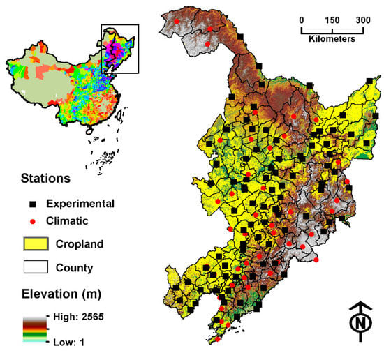
Figure 1.
Experimental (N = 89) and climatic (N = 83) station networks in Northeast China from 2001 to 2010. The underlying digital terrain is derived from the SRTM 90 m global elevation dataset [30]. The cropland layer is extracted from ESA CCI v1.3 land cover maps [29]. Inset: Maize crop area per county in 2005, based on agricultural census data from the Ministry of Agriculture.
2.1.2. Ground-Observed Crop Phenology and Climatic Data
Ground observations of crop phenology from 2001 to 2010 were obtained from the Agrometeorological Experimental Station Network operated by the China Meteorological Administration (http://data.cma.cn/en, accessed on 1 May 2015). Crop phenological observations were made on experimental plots following the Network’s standard guidelines [31]. Crops and varieties commonly grown in local regions were included in the experimental plots of a station under regional-representative crop management practices. Critical phenological events such as sowing, seedling, jointing, ripening, etc. during the crop cycle of spring maize, soybean, single rice, spring wheat, potato, etc. were observed. Two dates were recorded for each phenophase: one at the first appearance of the event and the other when the event was evident for at least 50% of the plants in the experimental plot. To match the satellite data, the second date of the seedling and the ripening phase was used to represent the start and end of the crop growing season, respectively. For rice, the transplanting phase was used in place of the seedling. In total, 24,808 records were collected from 89 stations in the NEC (Table 1).

Table 1.
Cropping structure, temperature threshold, and growing season of major crops in Northeast China from 2001 to 2010.
In addition to the agrometeorological stations, daily climatic data were also obtained from 83 climatic stations in the NEC from 2001 to 2010. The following parameters were used: air pressure (AP), mean daily temperature (TA), mean daily maximum temperature (TM), mean daily minimum temperature (TX), water vapor pressure (VP), relative humidity (RH), cloud cover (CL), wind velocity (UW), and precipitation (PR). The daily solar radiation (RA) data were separately obtained from [32].
In addition to temperature, the accumulative thermal units, or growing degree-days (GDD), were used to better account for the thermal conditions under which crops were grown. GDD was derived from temperature metrics using Equation (1):
where TB is the base temperature, the max function returns [(TM + TX)/2 − TB] if (TM + TX)/2 > TB or otherwise 0, and n is the duration of the calculation period in days. For field crops, 0 °C and 10 °C are two commonly used TB thresholds [33]. Considering that base-10 crops (i.e., spring maize, single rice, and potato) took a much larger share in harvest area than base-0 crops (i.e., soybean and spring wheat) in NEC (Table 1), GDD on the base temperature of 10 °C (or GDD10) was adopted in this analysis.
2.1.3. Crop Composition and Census Data
The annual harvest area of field crops at the county level from 2001 to 2010 was obtained as a part of the agricultural census dataset from the Ministry of Agriculture. This dataset represents the best-available, spatial-explicit crop production data in China at present (Figure 1, inset). Crop area composition was compiled per year for each of the 184 counties in NEC. The inset map in Figure 1 shows maize crop area per county in 2005 as an example. Figure 2 shows an aggregated composition pattern of these crops at the regional level in NEC.
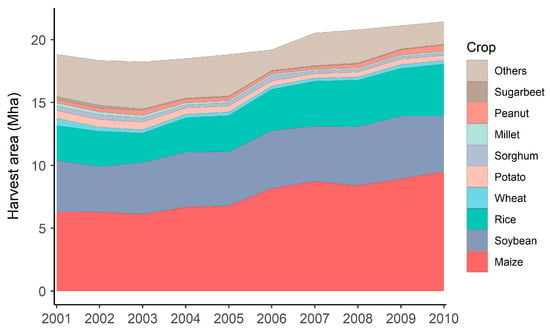
Figure 2.
Harvest area of major crops in Northeast China from 2001 to 2010. Mha, million hectares.
2.2. Methods
2.2.1. Methodological Overview
We modeled the satellite-ground difference of cropland SOS and EOS by multiple nonlinear regression using climatic parameters per agronomic experimental station. To obtain the satellite-ground difference, we adopted a buffer zone approach for the derivation of the average satellite- and ground-observed SOS and EOS at each station. We also crafted a procedure to determine the optimal size of the buffer zone. The obtained CTF was validated before being used in cropland LOS predictions in the NEC. To be more specific, the research was conducted in five steps (Figure 3): (1) A circular buffer zone was established around each experimental station in ArcGIS software following the buffer size optimization procedure detailed in Section 2.2.3; (2) The difference between the remote-sensed and ground-observed phenophase onsets was derived by deducting the ground-observed onset from the MODIS-derived onset. Two phenophases were considered, namely the SOS and EOS, to determine the LOS; (3) A regression model was established in the form of a second-order polynomial function to relate the satellite-ground difference of SOS or EOS to climatic factors that were separately identified in a correlation analysis. The second-order polynomial function was adopted to reflect the nonlinear relationship between climate and phenology [35]. We introduced the term climotransfer function (CTF) for the regression model obtained here in recognition of the role of climatic parameters in LSP calibration; (4) The CTF was validated and subsequently applied to the yearly MCD12Q2 dataset from 2001 to 2010 for croplands in NEC at the pixel scale to calibrate the MODIS-derived cropland growing season using gridded climatic parameters; (5) The cropland LOS change patterns during 2001–2010 in NEC were characterized and effects of climate change evaluated.
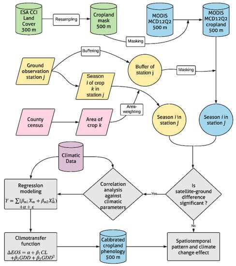
Figure 3.
The flowchart of the methodological approach.
2.2.2. Satellite-Ground Observational Difference
The satellite-ground observational difference of phenophase S, ∆S, at agricultural experimental station j, is derived using Equation (2):
where MOD is the average MODIS-derived onset of phenophase S, and GRD is the average ground-observed onset of phenophase S. GRD can be obtained from Equation (3):
where SGRD(k) is the ground-observed onset of phenophase S for crop k and Ak is the harvest area of crop k. To determine MOD(j), a circular buffer zone was created around station j and used to mask the MCD12Q2 dataset. The arithmetic mean of the MCD12Q2 pixel values was derived to represent MOD:
where p is a pixel and N is the total number of cropland pixels within the buffer zone.
2.2.3. Buffer Size Determination
The optimal buffer size was determined in three steps (Figure 4). Firstly, buffers with incremental radius r = 0, 0.5, 1.0, 1.5,…, 10.0 km were created for each of the 89 stations in ArcGIS version 10 software (ESRI, Redlands, CA, USA). Secondly, the mean onset (i.e., in Equation (2)) was computed from the pixel values within the buffer zone on a per buffer size per station basis using Equation (4). The change in mean onset at each radius increment was also computed. Thirdly, the optimal buffer size was determined when the following two conditions were simultaneously satisfied. The first condition was that the average onset change taking all stations together tended to minimize at values ≤ 1 d for each radius increment. The second condition was that the count of valid stations tended to maximize. A station was regarded as valid if at least one cropland pixel was present within the buffer zone.
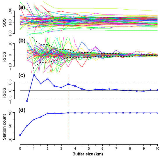
Figure 4.
The optimal buffer size determination, taking MODIS-derived cropland SOS in 2005 as an example. (a) Station-specific SOS variations against the buffer size. Each station is represented by a distinct color; (b) SOS change (δSOS) at each buffer size increment; (c) average SOS change (SOS) per buffer size increment; and (d) the count of valid stations. The vertical dotted line represents the obtained optimal buffer size.
2.2.4. Model Evaluation
The selection of the best-performing climotransfer functions was based on the performance evaluation of the candidate functions using a range of statistical metrics, including the mean absolute error (MAE), the mean absolute percentage error (MAPE), and the root-mean-square error (RMSE), which were given by Equations (5) through (7):
where y is the satellite-ground difference in phenophase onset, is the function estimate of y, and N is the total number of observations.
In addition, the coefficient of determination (R2), the Akaike information criterion (AIC), and the Bayesian information criterion (BIC) were also considered in the model evaluation. R2 provided a measurement of the function’s goodness of fit, whereas AIC and BIC accounted for the function’s complexity. These metrics were obtained using Equations (8) through (10), respectively:
where y, and N have the same meaning as in Equations (5)–(7), is the mean of y, and k is the number of parameters in the regression equation.
2.2.5. Data Analysis
Data processing and analyses were conducted using the R software [36]. In particular, the least-significant difference (LSD) method [37] was employed to test whether the MODIS-derived phenophase onset was statistically different from the ground-observed onset, while Pearson’s correlation coefficient and least squares were used to relate the satellite-ground observational difference to climatic factors and subsequently characterize the CTF, respectively.
3. Results
3.1. Optimal Buffer Size
The buffer size was optimized at a radius of r = 3.5 km following the procedure presented in Figure 4.
3.2. Satellite-Ground Difference
The MODIS-derived SOS onset per station compared well to the ground-observed onset when taking all 89 stations together from 2001 to 2010; however, a substantial delay was found in the MODIS-derived EOS onset, relative to the ground-observed date (Figure 5). The MODIS-derived mean onsets of SOS and EOS were evaluated as 143.1 and 279.7 doys, whereas the mean onsets of SOS and EOS by ground observation were characterized as 142.3 and 264.2 doys, respectively, meaning that the satellite-ground observational difference was 0.8 d for SOS and 15.5 d for EOS.
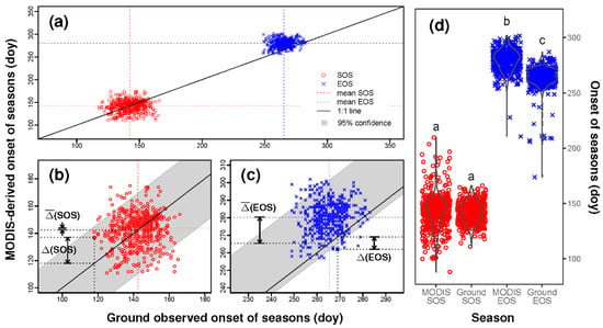
Figure 5.
Comparison between the MODIS-derived and the ground-observed onsets of the start (SOS) and end (EOS) of the cropland growing season from 2001 to 2010 in Northeast China. (a) Scatterplot with the 1:1 line and the mean MODIS-derived versus ground-observed dates; (b,c) Enlargement showing the MODIS-ground difference in SOS and EOS at a given station (∆SOS and ∆EOS) and the mean difference (SOS and EOS); (d) Violin plots showing the data distribution of the MODIS-derived against the ground-observed SOS and EOS. Different letters above the violin plots indicate a significant difference (p < 0.001).
We conducted variance analysis in combination with the LSD test [37] to judge whether this satellite-ground difference had statistical significance. The results (Figure 5d) showed that the MODIS-derived SOS was not significantly different from the ground-observed SOS. The results also showed, however, that the satellite-ground difference in EOS was significantly greater than zero. It means that MODIS-derived measurements show a significantly longer LOS than the observed data.
3.3. Correlation Analysis
We conducted the correlation analysis to relate the satellite-ground difference in EOS (i.e., ∆EOS) to common climatic factors (Table S1 in Supplementary Materials). Among the 17 climatic factors analyzed, the lower cloud cover (CL), wind velocity (UW), and growing degree days (GDD10) were found to have strong associations with ∆EOS (Figure 6). More specifically, GDD10 and CL were found to be positively associated with ∆EOS, whereas a negative association was found for UW. The Pearson correlation coefficients were evaluated as 0.64, 0.62, and −0.46 for GDD10, CL, and UW, respectively, against ∆EOS at the highest significance levels (p < 0.0001).
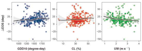
Figure 6.
Relationships between the satellite-ground difference in the cropland growing season end (∆EOS) and the major climatic factors, including the growing degree-days at the base temperature of 10 °C (GDD10), the lower cloud cover (CL), and the wind velocity (UW). Black lines represent the best-fit trends based on local polynomial regression.
3.4. Model Discrimination
The evaluation results of the performance of candidate CTF models in terms of prediction accuracy and goodness of fit are given in Table 2. In total, 12 candidate models were evaluated. It was found that GDD10 was the most reliable predictor of ∆EOS. All candidate models that included a GDD10 term performed better than the models that did not. It was also found that the top three best-performing models shared a similar function form that consisted of two climatic factors, one in quadratic form and the other in linear form. Model #3 in Table 2, for example, is ranked first by the criterion of the coefficient of determination (R2). However, it suffered from being more complex than, e.g., model #2, as indicated by the higher AIC and BIC values for model #3. Although model #1 ranked the second in terms of model simplicity and the fourth in terms of the goodness of fit, it ranked the first in terms of prediction accuracy. Overall, model #1 was evaluated as the best-performing model and hence was adopted as the climotransfer function for subsequent analysis in this paper.

Table 2.
Performance of the candidate climotransfer function models. Numbers in parentheses are model rankings per criterion. The sum of the rankings per row is given as a model’s overall score in the right-most column. Lower scores mean higher performances. R2, coefficient of determination; AIC, Akaike information criterion; BIC, Bayesian information criterion; RMSE, root mean square error; MAE, mean absolute error; MAPE, mean absolute percentage error.
Model #1 is given in Equation (11). It is also presented in Figure 7 with two-dimensional plots for the model’s nonlinear and linear terms, respectively.
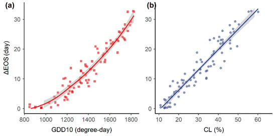
Figure 7.
Two-dimensional representation of the climotransfer function developed in this paper (Equation (11)) based on a simultaneous characterization of ΔEOS’ nonlinear and linear responses to growing degree-days (a) and cloud cover (b).
3.5. Model Validation
We employed two cross-validation approaches in an attempt to validate the obtained climotransfer function. In the first approach, which is known as 50–50 cross-validation, the ground observation stations were split into two equal subsets. One subset was used to train the CTF, and the other was used to validate the CTF’s predictions. In the second approach, which is known as leave-one-out cross-validation (LOOCV), one station was left out as the validation data, while the rest of the stations were used in model training. This process was repeated until every station had been used once as validation data. The CTF-predicted ∆EOS values were plotted against the ground-observed ∆EOS in Figure 8. The results showed that the CTF predictions compared well to ground observations in both approaches. The mean observed and the mean predicted ∆EOS values were centered and coincided with the 1:1 line. Moreover, no sensible patterns were discernible in the scatter plots in Figure 8, meaning that variations in ∆EOS were adequately characterized and the presence of systematic biases in CTF predictions was highly unlikely. Nevertheless, it was worth indicating that the prediction errors were systematically smaller with the LOOCV than with the 50–50 approach. The trend line fitted to the predicted against the observed ∆EOS was evaluated to have an intercept closer to zero in LOOCV than in 50–50 (−0.99 versus −1.23 d, respectively) and a slope closer to one (1.07 versus 1.22), suggesting that the CTF prediction error was inversely proportional to the size of the training dataset.
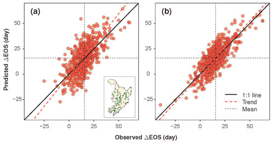
Figure 8.
Comparison between the model-predicted versus station-characterized ∆EOS using 50–50 (a) and leave-one-out cross-validation methods (b). The inset figure in (a) shows the spatial setting of the stations used in model training (solid dots, 50%) and model validation (hollow squares, 50%). The regression equations of the trend lines are (a) and (b).
3.6. Cropland Phenology
Annual onsets of the start, end, and length of the cropland growing season in Northeast China, both before and after calibration, are presented in Figure 9. Station-specific and overall changes in cropland growing seasons from 2001 to 2010 are presented in Figure 10. Summary statistics are given in Table S2.
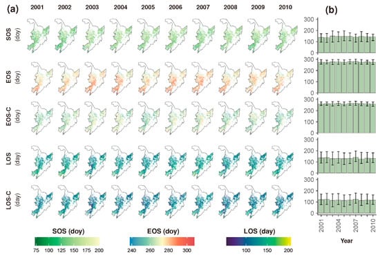
Figure 9.
(a) The start (SOS), end (EOS), and length (LOS) of the cropland growing season in Northeast China (NEC) based on the MCD12Q2 land surface phenology product. EOS-C and LOS-C are calibrated EOS and LOS, respectively, using the climotransfer function developed in this paper; (b) The annual mean and 95% confidence interval of SOS, EOS, EOS-C, LOS, and LOS-C in the NEC from 2001 to 2010. Data are given in Table S2.
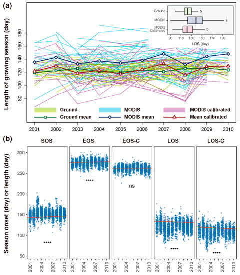
Figure 10.
(a) Temporal variations in cropland growing season length (LOS) per station in Northeast China from 2001 to 2010. Each thin line represents a station. Each thick line with hollow markers represents the mean of all stations. Inset: Overall comparison between ground-observed and MODIS-derived versus climotransfer function-calibrated LOS. Boxplots with different lower-case letters indicate a significant difference (p < 0.001); (b) Temporal trend (solid line) in the cropland growing season based on annual time series (clustered dots) of the season start (SOS), end (EOS), and length (LOS) at the pixel scale. EOS-C and LOS-C are calibrated EOS and LOS, respectively. ****, p < 0.0001; ns, not significant.
The cropland growing season in Northeast China largely remained stable from 2001 to 2010 (Figure 9). Although the pixel values of SOS, for instance, varied across a wide range from 34 to 239 doy according to the MODIS data, the corresponding interquartile range (IQR) of these values was much narrower. The IQR was evaluated as 25.3 d for SOS, contrasting the minimum-maximum range of 205 d (Table 3). On average, the cropland growing season started at 144.5 doy (i.e., 25 May) and ended at 276.8 doy (i.e., 4 October) according to the uncalibrated MODIS data. In comparison, the CTF model prediction showed that the calibrated ending date of the cropland growing season was 262.4 doy, which was 14.4 d earlier than the uncalibrated EOS. Accordingly, the length of the cropland growing season was calibrated from 132.2 d to 117.8 d.

Table 3.
Summary statistics and the least significant difference test results for the onset and length of the cropland growing season in Northeast China from 2001 to 2010 as influenced by calibration. EOS-C, calibrated end-of-season onset; LOS-C, calibrated length of the growing season.
Has the CTF calibration produced statistically significant differences in the phenophase and duration of the cropland growing season? We employed the LSD test [37] to answer this question. The testing results (Table 3) confirmed that the calibrated EOS and LOS (i.e., EOS-C and LOS-C, respectively) were both significantly different from their uncalibrated counterparts, as also illustrated by the maps and the bar plots in Figure 9.
3.7. Latitudinal Gradient
We evaluated the latitudinal gradient in cropland LOS change in the NEC from 2001 to 2010 (Figure 11). The results showed that cropland LOS tended to be longer in lower latitudes and shorter in higher latitudes. This latitudinal pattern was supported both by ground observations and by MODIS data. However, the ground observations and MODIS data supported different gradient values. The latitudinal gradient characterized based on ground observations was −1.19 d degree−1 of latitude northward, contrasting with a gradient of −2.98 d degree−1 based on MODIS data, while the gradient evaluated with the climotransfer function-predicted LOS was −1.68 d degree−1 of latitude northward. The LSD-tests showed that the climotransfer function-predicted gradient was not significantly different from the gradient supported by ground observations (p > 0.05), whereas the MODIS data-characterized gradient was significantly different from the latter (p < 0.01).
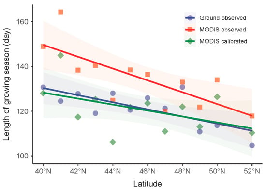
Figure 11.
The relationship between the length of the cropland growing season (LOS) and the latitude in Northeast China from 2001 to 2010. The regression equations of the trend lines are: for ground-observed LOS, for MODIS-observed LOS, and for climotransfer function-predicted LOS, p < 0.0001.
4. Discussion
4.1. Factor Characterization
Our results of factor analysis confirmed that temperature played a dominant role in cropland phenology in the NEC during the first decade of the 21st century. Among the nine climatic factors that passed the statistical significance test (p < 0.05), five were temperature-related, including TA, TM, TX, GDD0, and GDD10. The reasons to adopt GDD10 in the final CTF were twofold. On the one hand, GDD10 was widely used in practice with a clear agronomic meaning, while, on the other hand, its correlation with the satellite-ground difference in EOS was among the highest. It is worth noting that cloud cover and wind velocity were tested significantly, whereas precipitation was not. It is well understood that temperature is a major driver of many biological processes, ranging from enzyme-catalyzed reactions to membrane fluidity [38]. In many cases, a higher rate in plant development is observed with higher temperatures, leading to an earlier switch to the next phenophase [39]. Conversely, in water-limited systems, plants enter dormancy or die when soil water becomes scarce or depleted to sub-wilting point levels [40]. It is, therefore, not a surprise that precipitation failed the significance test because precipitation was largely not a limiting factor for crop production in this temperate subhumid region of the NEC. Precipitation would be significantly lower in more arid regions, e.g., in Northwestern China [41].
Our contribution to the factor analysis was that we characterized the lower cloud cover as an additional driver of crop phenology, which was, to our knowledge, seldom established in previous modeling efforts. A deeper understanding of the cloud cover’s role in crop phenology, as well as in satellite remote sensing is still lacking and, hence, deserves more attention.
4.2. Cropland Growing Season Change
Previous research has found that crop cycles may either be shortened or prolonged at decadal time scales in the face of climate change [42]. Observed data from China during 1992–2018 showed that the soybean growing season was shortened by 1.3 d decade−1, resulting from a significant delay in the sowing date (1.0 d decade−1) and a slight advance in the maturity date (−0.3 d decade−1) [43]. Also at the national scale in China, Luo et al. found that the maize growing season was slightly prolonged by 0.6 d decade−1 from 1981 to 2018 [44] because the maize sowing and maturity dates were both delayed at differing rates of 0.6 and 1.2 d decade−1, respectively. In contrast, evidence from NEC showed an opposite trend at the start of the rice growing season. Based on data obtained during 1981–2009, Tao et al. [45] suggested that the rice transplanting date advanced significantly by 1.4 d decade−1, whereas a delay of 1.3 d decade−1 was found in the crop’s maturity date, thus prolonging the growing season by 2.7 d decade−1. Furthermore, our results provided further evidence showing the complexity of cropland phenology change.
On the one hand, our results supported a shortened season length, but on the other hand, although our results suggested a delay in SOS, no trend was supported for EOS based on our CTF-calibrated MODIS data. According to the characterized temporal trends (Table 4), cropland SOS in NEC delayed significantly at a rate of 4.5 d decade−1 from 2001 to 2010, whereas the CTF-calibrated EOS only showed a slight delay of 0.015 d decade−1 (p > 0.05). Overall, cropland LOS in NEC was shortened by 4.5 d decade−1 during 2001–2010. Although our finding of a substantially delayed SOS was in agreement with Tan et al. and Luo et al. [43,44], the magnitude of the delay in this study was much larger. It is interesting to observe that few previous studies reported a neutral trend for EOS, showing the uniqueness of our results. Moreover, the shorter growing season in our results was in line with that of Tan et al. [43], but the magnitude of change in our results was much larger. The difference was, though, that our results were obtained from multiple crops, whereas Tan et al.’s were from a single crop.

Table 4.
Annual mean values of and temporal trends (day year−1) at the start (SOS), end (EOS), and length of the cropland growing season (LOS) in Northeast China from 2001 to 2010. The trend is evaluated as the linear slope term fitted to the growing season time series at the pixel scale.
The results of the phenological change discussed above are largely in agreement with expected patterns of LOS change under global climate change. A longer growth period was widely observed in natural vegetation, as a result of an earlier start and a delayed end that are mainly driven by rising temperatures [1,24]. However, in cropland systems, the dynamics of growing season change are jointly controlled by both environmental and anthropogenic factors. The temperature remains the major environmental factor, whereas cultivar shifts represent one of the most influential anthropogenic factors [42]. Under rising temperature regimes, crops’ thermal requirements are satisfied in a shorter time—hence a shortening trend in LOS [43]. However, because of shifts in planting dates and/or adoption of longer-duration cultivars, field crops also show prolonged growth duration despite the warming trends [46]. In this paper, the study period was relatively short (~10 years), and the characterized LOS change was dominated by the current cultivars, not the new cultivars. The replacement of the current cultivars was in progress; however, the area of new cultivars was not yet comparable to that of the current cultivars. As a result, cultivar shift had yet to dominate the overall LOS trend.
Not only our results are unique, our approach is unique as well. Statistical models developed with data from multiple stations were documented to be better at predicting crop response to climate change than the time series model at single stations [47]. Therefore, rather than trying to characterize the LOS change patterns at the station scale, we opted to aggregate the stations together in NEC to analyze the temporal changes at the regional scale. Moreover, statistical approaches are frequently limited by the quantity and quality of data used to train models, which results in fairly large uncertainties. Relatively few studies have devoted long-term crop trial data to examine how satellite observations are different from synchronous observations in the field [48]. Importantly, historical crop trial data, with more accurate records of phenology, yield, cultivar, and management, allowed us to study how a statistical model could be developed to calibrate the satellite data for more accurate spatiotemporal monitoring of cropland phenology.
4.3. The Calibration Imperative
The model developed in this paper produced statistically significant improvements to the MODIS-derived cropland phenology in alignment with ground observations. The LSD tests showed that the CTF-predicted LOS was significantly shorter than the MODIS-derived LOS. The difference of 14.4 d not only showed that the calibration itself was valid but also suggested that careful calibration of satellite-observed cropland phenology had important implications for, e.g., climate change and food security-related decision making.
Previous research has revealed that the productivity of both natural vegetation and cropland systems is closely associated with the LOS. In North China Plain, for example, a maize yield increase of 72.5 kg ha−1 was observed for every 1 d lengthening of the crop’s growth period from 1981 to 2007 [18]. It is clear that an overreported cropland LOS may lead to false optimism in crop yield projections, showing how important LOS calibration is for unbiased food security decision-making [49,50]. Moreover, LOS calibration is also important in climate change attribution based on vegetation- or cropland-related indicators. For example, Huang et al. measured the poleward advancement pace of the isolines of vegetation growing season mean temperature (i.e., GST velocity) over the northern latitudes (>50 °N) based on MODIS data [51]. A GST velocity of 5.4 ± 1.0 km yr−1 was estimated for the period 1982–2011. Whether the MODIS-derived vegetation phenology is balanced for natural vegetation is out of the scope of this paper; however, the overestimation of cropland LOS by MODIS would have led to an underestimated GST velocity if it had been evaluated on croplands, since the LOS underestimation may likely be higher in lower latitudes and lower in higher latitudes. However, can the CTF calibration model make a distinction if a similar climate change indicator is to be evaluated on cropland in the NEC?
Our LOS latitudinal gradient evaluation results confirmed that the gradient supported by the calibrated MODIS data was not statistically different from the gradient obtained from the ground observation data (1.68 versus 1.19 d degree−1, p > 0.05). Therefore, confidence was attached to the estimated shortening of the cropland growing season by 1.68 days per degree of latitude northward. Without calibration, however, this gradient would be overestimated by 77%. Although this calibrated gradient was lower than the gradient of 4 d degree−1 as stipulated by the “Hopkins bioclimatic law” [52], the latter was established based on data collected from North American forests, an ecosystem different in type and location from croplands of northeastern Asia. There was no doubt that LOS calibration using the CTF model developed in this paper produced a significantly more accurate estimation of the LOS latitudinal gradient.
Given these notable differences, we would like to call attention to the need for calibration of satellite LSP products before any meaningful applications in, e.g., climate change and food security. It is important to note that NEC is China’s most climate-change-impacted grain production region, whose grain output accounts for one-fifth of the national total [53,54]. Improved characterization of LOS change in field crops involving climate shocks in this vast region, which is equivalent in land mass to France and Germany combined, undoubtedly will better inform climate change and food security decision-making at regional and national scales [2,55].
4.4. Uncertainties
Our results are subject to uncertainties originating from a range of sources. Firstly, the mismatch between the MODIS and the ground observation data persisted, despite the buffer optimization efforts. Although a cropland mask was applied to minimize the influence of other land-use types, misclassification could not be ruled out, especially for stations near urban areas. In addition to the classic “point versus pixel” problem [22], the mixture of crop species posed extra challenges. The likelihood of a mixture is usually higher in China, where the field size is typically smaller than that in North America or Europe [41]. Even with the same crop species, temperature requirements differ widely across simultaneous cultivars and their adaptive capacities to a changing environment [34,56]. Therefore, in agroclimatic regions other than the NEC where multi-cropping dominates, such as the North China Plain, crop-specific CTFs would be more appropriate than a single CTF. Ideally, function parameters are re-estimated for each of the eight agroclimatic regions [57] in China. Secondly, the lack of a mechanistic understanding of the climatic factors’ roles in crop phenology limited our modeling effort. The effect of CL, or photoperiod length, on crop development is species-dependent; its magnitude is believed to be substantially smaller than that of TA or PR [5]. However, the association of CL with crop phenology is much scarcer in the literature than, e.g., TA and PR. More attention is therefore needed to help establish process-level links with crop development. Thirdly, the spatial pattern in the agrometeorological station network gives rise to additional errors. In recent years, the stations are becoming increasingly associated with rapid urbanization. As a result, the representability of these stations for croplands tends to decrease, as evidenced by the large buffer size of 3.5 km found in this study. If relocation is possible, the modeling error is expected to decrease with a decreasing buffer size.
5. Conclusions
We developed a climotransfer function for satellite LSP data calibration. Although only one CTF was developed, multiple CTFs might be necessary, as indicated by our proposed modeling flowchart. With the CTF-calibrated MODIS LSP data, we have found a shortening trend of 4.5 d decade−1 and a northward latitudinal gradient of −1.6 d degree−1 for croplands in Northeast China from 2001 to 2010. We have also demonstrated that these spatiotemporal patterns would have been erroneously characterized if calibration had not been applied. Hence, we call for more attention to the proper calibration of satellite LSP products before any applications of potential importance, e.g., in climate change and food security.
Supplementary Materials
The following supporting information can be downloaded at: https://www.mdpi.com/article/10.3390/rs15010072/s1, Table S1: Correlation analysis between the satellite-ground difference in EOS and climatic parameters. In-season (MJJAS) climatic parameter values are used. The correlation coefficient (r) and probability (p) are reported for each climatic parameter; Table S2: Annual onsets of the start, end, and length of the MODIS-derived cropland growing season in Northeast China from 2001 to 2010. LCL and UCL are the lower and upper limits of the 90% confidence interval.
Author Contributions
Conceptualization, L.Y.; methodology, L.Y.; software, L.Y.; validation, L.Y. and L.X.; formal analysis, J.D.G. and E.V.R.; investigation, L.Y.; resources, J.D.G. and L.X.; data curation, L.X.; writing—original draft preparation, L.Y.; writing—review and editing, E.V.R.; visualization, L.Y.; supervision, J.D.G.; project administration, E.V.R.; funding acquisition, L.X. All authors have read and agreed to the published version of the manuscript.
Funding
The APC was funded by Yunnan Lijun Xu’s expert workstation, grant number: 202005AF1500742 and the Yunnan Key Research and Development Program, grant number: 202003AD150016.
Data Availability Statement
The MODIS Land Cover Dynamics data product MCD12Q2 (Collection 6) is freely available at the USGS Land Processes DAAC web portal (https://lpdaac.usgs.gov/, accessed on 1 December 2021). The European Space Agency’s CCI-LC land cover dataset is available at http://maps.elie.ucl.ac.be/CCI/viewer/index.php, accessed on 1 December 2021. Climatic and agrometeorological observational data are available at the China Meteorological Data Service Center (http://data.cma.cn/en, accessed on 1 December 2021). Crop harvest area data at the provincial level are available at http://www.stats.gov.cn/english/Statisticaldata/AnnualData/, accessed on 1 December 2021.
Conflicts of Interest
The authors declare no conflict of interest.
References
- Menzel, A.; Fabian, P. Growing season extended in Europe. Nature 1999, 397, 659. [Google Scholar] [CrossRef]
- Settele, J.; Scholes, R.; Betts, R.; Bunn, S.E.; Leadley, P.; Nepstad, D.; Overpeck, J.T.; Taboada, M.A. Terrestrial and inland water systems. In Climate Change 2014: Impacts, Adaptation, and Vulnerability. Part A: Global and Sectoral Aspects. Contribution of Working Group II to the Fifth Assessment Report of the Intergovernmental Panel of Climate Change; Field, C.B., Barros, V.R., Dokken, D.J., Mach, K.J., Mastrandrea, M.D., Bilir, T.E., Chatterjee, M., Ebi, K.L., Estrada, Y.O., Genova, R.C., et al., Eds.; Cambridge University Press: Cambridge, UK; New York, NY, USA, 2014; pp. 271–359. [Google Scholar]
- Garonna, I.; de Jong, R.; Schaepman, M.E. Variability and evolution of global land surface phenology over the past three decades (1982–2012). Glob. Chang. Biol. 2016, 22, 1456–1468. [Google Scholar] [CrossRef] [PubMed]
- Reyes-Fox, M.; Steltzer, H.; Trlica, M.J.; McMaster, G.S.; Andales, A.A.; LeCain, D.R.; Morgan, J.A. Elevated CO2 further lengthens growing season under warming conditions. Nature 2014, 510, 259–262. [Google Scholar] [CrossRef] [PubMed]
- Badeck, F.-W.; Bondeau, A.; Bottcher, K.; Doktor, D.; Lucht, W.; Schaber, J.; Sitch, S. Responses of spring phenology to climate change. New Phytol. 2004, 162, 295–309. [Google Scholar] [CrossRef]
- Zhang, X.; Friedl, M.A.; Schaaf, C.B. Global vegetation phenology from Moderate Resolution Imaging Spectroradiometer (MODIS): Evaluation of global patterns and comparison with in situ measurements. J. Geophys. Res. 2006, 111, G04017. [Google Scholar] [CrossRef]
- Cong, N.; Wang, T.; Nan, H.; Ma, Y.; Wang, X.; Myneni, R.B.; Piao, S. Changes in satellite-derived spring vegetation green-up date and its linkage to climate in China from 1982 to 2010: A multimethod analysis. Glob. Chang. Biol. 2013, 19, 881–891. [Google Scholar] [CrossRef]
- Jeong, S.-J.; Ho, C.-H.; Gim, H.-J.; Brown, M.E. Phenology shifts at start vs. end of growing season in temperate vegetation over the Northern Hemisphere for the period 1982–2008. Glob. Chang. Biol. 2011, 17, 2385–2399. [Google Scholar] [CrossRef]
- White, M.A.; de Beurs, K.M.; Didan, K.; Inouye, D.W.; Richardson, A.D.; Jensen, O.P.; O’Keefe, J.; Zhang, G.; Nemani, R.R.; van Leeuwen, W.J.D.; et al. Intercomparison, interpretation, and assessment of spring phenology in North America estimated from remote sensing for 1982–2006. Glob. Chang. Biol. 2009, 15, 2335–2359. [Google Scholar] [CrossRef]
- Templ, B.; Koch, E.; Bolmgren, K.; Ungersböck, M.; Paul, A.; Scheifinger, H.; Rutishauser, T.; Busto, M.; Chmielewski, F.-M.; Hájková, L.; et al. Pan European Phenological database (PEP725): A single point of access for European data. Int. J. Biometeorol. 2018, 62, 1109–1113. [Google Scholar] [CrossRef]
- Seyednasrollah, B.; Young, A.M.; Hufkens, K.; Milliman, T.; Friedl, M.A.; Frolking, S.; Richardson, A.D. Tracking vegetation phenology across diverse biomes using Version 2.0 of the PhenoCam Dataset. Sci. Data 2019, 6, 222. [Google Scholar] [CrossRef]
- Peng, D.; Zhang, X.; Wu, C.; Huang, W.; Gonsamo, A.; Huete, A.R.; Didan, K.; Tan, B.; Liu, X.; Zhang, B. Intercomparison and evaluation of spring phenology products using National Phenology Network and AmeriFlux observations in the contiguous United States. Agric. For. Meteorol. 2017, 242, 33–46. [Google Scholar] [CrossRef]
- Tian, F.; Cai, Z.; Jin, H.; Hufkens, K.; Scheifinger, H.; Tagesson, T.; Smets, B.; Van Hoolst, R.; Bonte, K.; Ivits, E.; et al. Calibrating vegetation phenology from Sentinel-2 using eddy covariance, PhenoCam, and PEP725 networks across Europe. Remote Sens. Environ. 2021, 260, 112456. [Google Scholar] [CrossRef]
- Ye, L.; Tang, H.; Wu, W.; Yang, P.; Nelson, G.C.; Mason-D’Croz, D.; Palazzo, A. Chinese food security and climate change: Agriculture futures. Economics 2014, 8, 1. [Google Scholar] [CrossRef]
- Porter, J.R.; Xie, L.; Challinor, A.J.; Cochrane, K.; Howden, S.M.; Iqbal, M.M.; Lobell, D.B.; Travasso, M.I. Food security and food production systems. In Climate Change 2014: Impacts, Adaptation, and Vulnerability. Part A: Global and Sectoral Aspects. Contribution of Working Group II to the Fifth Assessment Report of the Intergovernmental Panel of Climate Change; Field, C.B., Barros, V.R., Dokken, D.J., Mach, K.J., Mastrandrea, M.D., Bilir, T.E., Chatterjee, M., Ebi, K.L., Estrada, Y.O., Genova, R.C., et al., Eds.; Cambridge University Press: Cambridge, UK; New York, NY, USA, 2014; pp. 485–533. [Google Scholar]
- Smith, P.; Bustamante, M.; Ahammad, H.; Clark, H.; Dong, H.; Elsiddig, E.A.; Haberl, H.; Harper, R.; House, J.; Jafari, M.; et al. Agriculture, forestry and other land use (AFOLU). In Climate Change 2014: Mitigation of Climate Change. Contribution of Working Group III to the Fifth Assessment Report of the Intergovernmental Panel on Climate Change; Edenhofer, O., Pichs-Madruga, R., Sokona, Y., Farahani, E., Kadner, S., Seyboth, K., Adler, A., Baum, T., Brunner, S., Eickemeier, P., et al., Eds.; Cambridge University Press: Cambridge, UK; New York, NY, USA, 2014; pp. 811–922. [Google Scholar]
- Tao, F.; Yokozawa, M.; Xu, Y.; Hayashi, Y.; Zhang, Z. Climate changes and trends in phenology and yields of field crops in China, 1981–2000. Agric. For. Meteorol. 2006, 138, 82–92. [Google Scholar] [CrossRef]
- Zhao, J.; Yang, X.; Dai, S.; Lv, S.; Wang, J. Increased utilization of lengthening growing season and warming temperatures by adjusting sowing dates and cultivar selection for spring maize in Northeast China. Eur. J. Agron. 2015, 67, 12–19. [Google Scholar] [CrossRef]
- Chen, S.; He, L.; Cao, Y.; Wang, R.; Wu, L.; Wang, Z.; Zou, Y.; Siddique, K.H.M.; Xiong, W.; Liu, M.; et al. Comparisons among four different upscaling strategies for cultivar genetic parameters in rainfed spring wheat phenology simulations with the DSSAT-CERES-Wheat model. Agric. Water Manag. 2021, 258, 107181. [Google Scholar] [CrossRef]
- Xu, L.; Ye, L.; Nie, Y.; Yang, G.; Xin, X.; Yuan, B.; Yang, X. Sown alfalfa pasture decreases grazing intensity while increasing soil carbon: Experimental observations and DNDC model predictions. Front. Plant Sci. 2022, 13, 1019966. [Google Scholar] [CrossRef]
- Chuine, I.; Régnière, J. Process-based models of phenology for plants and animals. Annu. Rev. Ecol. Evol. Syst. 2017, 48, 159–182. [Google Scholar] [CrossRef]
- Chen, X.; Wang, D.; Chen, J.; Wang, C.; Shen, M. The mixed pixel effect in land surface phenology: A simulation study. Remote Sens. Environ. 2018, 211, 338–344. [Google Scholar] [CrossRef]
- Tang, H.; Ye, L. Comparative Study on Methodology of Land Production Potential; China Agricultural Science and Technology Press: Beijing, China, 1997; p. 301. [Google Scholar]
- Zhang, X.; Friedl, M.A.; Schaaf, C.B.; Strahler, A.H. Climate controls on vegetation phenological patterns in northern mid- and high latitudes inferred from MODIS data. Glob. Chang. Biol. 2004, 10, 1133–1145. [Google Scholar] [CrossRef]
- Liu, X.; Zhu, X.; Pan, Y.; Zhu, W.; Zhang, J.; Zhang, D. Thermal growing season and response of alpine grassland to climate variability across the Three-Rivers Headwater Region, China. Agric. For. Meteorol. 2016, 220, 30–37. [Google Scholar] [CrossRef]
- Yao, Y.; Ye, L.; Tang, H.; Tang, P.; Wang, D.; Si, H.; Hu, W.; Van Ranst, E. Cropland soil organic matter content change in Northeast China, 1985–2005. Open Geosci. 2015, 7, 234–243. [Google Scholar] [CrossRef]
- Xia, T.; Wu, W.-B.; Zhou, Q.-B.; Verburg, P.H.; Yang, P.; Hu, Q.; Ye, L.-M.; Zhu, X.-J. From statistics to grids: A two-level model to simulate crop pattern dynamics. J. Integr. Agric. 2022, 21, 1786–1798. [Google Scholar] [CrossRef]
- Gray, J.; Sulla-Menashe, D.; Friedl, M.A. User Guide to Collection 6 MODIS Land Cover Dynamics (MCD12Q2) Product; NASA EOSDIS Land Processes DAAC: Missoula, MT, USA, 2019; p. 8. [Google Scholar]
- ESA. Land Cover CCI Product User Guide Version 2. Technical Report. 2017. Available online: https://maps.elie.ucl.ac.be/CCI/viewer/download/ESACCI-LC-Ph2-PUGv2_2.0.pdf (accessed on 1 September 2022).
- Farr, T.G.; Rosen, P.A.; Caro, E.; Crippen, R.; Duren, R.; Hensley, S.; Kobrick, M.; Paller, M.; Rodriguez, E.; Roth, L.; et al. The Shuttle Radar Topography Mission. Rev. Geophys. 2007, 45, RG2004. [Google Scholar] [CrossRef]
- China Meteorological Administration. Agro-Meteorological Observation Standard; China Meteorological Press: Beijing, China, 1993. [Google Scholar]
- Yang, K.; Koike, T.; Ye, B. Improving estimation of hourly, daily, and monthly solar radiation by importing global data sets. Agric. For. Meteorol. 2006, 137, 43–55. [Google Scholar] [CrossRef]
- Luo, Q. Temperature thresholds and crop production: A review. Clim. Chang. 2011, 109, 583–598. [Google Scholar] [CrossRef]
- Reilly, J.; Baethgen, W.; Chege, F.E.; van de Geijn, S.C.; Lin, E.; Iglesias, A.; Kenny, G.; Patterson, D.; Rogasik, J.; Röter, R.; et al. Agriculture in a changing climate: Impacts and adaptation. In Climate Change 1995: Scientific-Technical Analyses of Impacts, Adaptations, and Mitigation of Climate Change: Contribution of Working Group II to the IPCC Second Assessment Report; Watson, R.T., Zinyowera, M.C., Moss, R.H., Eds.; Cambridge University Press: Cambridge, UK, 1995; pp. 427–467. [Google Scholar]
- Pope, K.S.; Dose, V.; Da Silva, D.; Brown, P.H.; Leslie, C.A.; Dejong, T.M. Detecting nonlinear response of spring phenology to climate change by Bayesian analysis. Glob. Chang. Biol. 2013, 19, 1518–1525. [Google Scholar] [CrossRef]
- R Core Team. R: A Language and Environment for Statistical Computing, Version 4.1.3; R Foundation for Statistical Computing: Vienna, Austria, 2022; Available online: https://www.R-project.org/ (accessed on 1 May 2022).
- de Mendiburu, F. Agricolae: Statistical Procedures for Agricultural Research. R Package Version 1.3-5. 2021. Available online: https://CRAN.R-project.org/package=agricolae (accessed on 1 May 2022).
- Johnson, I.R.; Thornley, J.H.M. Temperature dependence of plant and crop process. Ann. Bot. 1985, 55, 1–24. [Google Scholar] [CrossRef]
- Saxe, H.; Cannell, M.G.R.; Johnsen, Ø.; Ryan, M.G.; Vourlitis, G. Tree and forest functioning in response to global warming. New Phytol. 2002, 149, 369–399. [Google Scholar] [CrossRef]
- Verdoodt, A.; Ranst, E.V.; Ye, L.; Verplancke, H. A daily multi-layered water balance model to predict water and oxygen availability in tropical cropping systems. Soil Use Manag. 2005, 21, 312–321. [Google Scholar] [CrossRef]
- Xu, L.; Li, D.; Wang, D.; Ye, L.; Nie, Y.; Fang, H.; Xue, W.; Bai, C.; Van Ranst, E. Achieving the dual goals of biomass production and soil rehabilitation with sown pasture on marginal cropland: Evidence from a multi-year field experiment in northeast Inner Mongolia. Front. Plant Sci. 2022, 13, 985864. [Google Scholar] [CrossRef] [PubMed]
- Bezner Kerr, R.; Hasegawa, T.; Lasco, R.; Bhatt, I.; Deryng, D.; Farrell, A.; Gurney-Smith, H.; Ju, H.; Lluch-Cota, S.; Meza, F.; et al. Food, fibre, and other ecosystem products. In Climate Change 2022: Impacts, Adaptation and Vulnerability. Contribution of Working Group II to the Sixth Assessment Report of the Intergovernmental Panel on Climate Change; Pörtner, H.-O., Roberts, D.C., Tignor, M., Poloczanska, E.S., Mintenbeck, K., Alegría, A., Craig, M., Langsdorf, S., Löschke, S., Möller, V., et al., Eds.; Cambridge University Press: Cambridge, UK; New York, NY, USA, 2022; pp. 713–906. [Google Scholar] [CrossRef]
- Tan, Q.; Liu, Y.; Dai, L.; Pan, T. Shortened key growth periods of soybean observed in China under climate change. Sci. Rep. 2021, 11, 8197. [Google Scholar] [CrossRef] [PubMed]
- Luo, Y.; Zhang, Z.; Zhang, L.; Zhang, J.; Tao, F. Weakened maize phenological response to climate warming weakened over 1981-2018 due to cultivar shifts. Adv. Clim. Chang. Res. 2022, 13, 710–720. [Google Scholar] [CrossRef]
- Tao, F.; Zhang, Z.; Shi, W.; Liu, Y.; Xiao, D.; Zhang, S.; Zhu, Z.; Wang, M.; Liu, F. Single rice growth period was prolonged by cultivars shifts, but yield was damaged by climate change during 1981-2009 in China, and late rice was just opposite. Glob. Chang. Biol. 2013, 19, 3200–3209. [Google Scholar] [CrossRef] [PubMed]
- Zhu, P.; Jin, Z.; Zhuang, Q.; Ciais, P.; Bernacchi, C.; Wang, X.; Makowski, D.; Lobell, D. The important but weakening maize yield benefit of grain filling prolongation in the US Midwest. Glob. Chang. Biol. 2018, 24, 4718–4730. [Google Scholar] [CrossRef]
- Lobell, D.B.; Burke, M.B. On the use of statistical models to predict crop yield responses to climate change. Agric. For. Meteorol. 2010, 150, 1443–1452. [Google Scholar] [CrossRef]
- Liu, L.; Wang, E.; Zhu, Y.; Tang, L. Contrasting effects of warming and autonomous breeding on single-rice productivity in China. Agric. Ecosyst. Environ. 2012, 149, 20–29. [Google Scholar] [CrossRef]
- Ye, L.; Yang, G.; Van Ranst, E.; Tang, H. Time-series modeling and prediction of global monthly absolute temperature for environmental decision making. Adv. Atmos. Sci. 2013, 30, 382–396. [Google Scholar] [CrossRef]
- Ye, L.-M.; Malingreau, J.-P.; Tang, H.-J.; Van Ranst, E. The breakfast imperative: The changing context of global food security. J. Integr. Agric. 2016, 15, 1179–1185. [Google Scholar] [CrossRef]
- Huang, M.; Piao, S.; Janssens, I.A.; Zhu, Z.; Wang, T.; Wu, D.; Ciais, P.; Myneni, R.B.; Peaucelle, M.; Peng, S.; et al. Velocity of change in vegetation productivity over northern high latitudes. Nat. Ecol. Evol. 2017, 1, 1649–1654. [Google Scholar] [CrossRef]
- Vitasse, Y.; Signarbieux, C.; Fu, Y.H. Global warming leads to more uniform spring phenology across elevations. Proc. Natl. Acad. Sci. USA 2018, 115, 1004–1008. [Google Scholar] [CrossRef] [PubMed]
- Xia, T.; Wu, W.; Zhou, Q.; Tan, W.; Verburg, P.H.; Yang, P.; Ye, L. Modeling the spatio-temporal changes in land uses and its impacts on ecosystem services in Northeast China over 2000-2050. J. Geogr. Sci. 2018, 28, 1611–1625. [Google Scholar] [CrossRef]
- Ye, L.; Yang, J.; Verdoodt, A.; Moussadek, R.; Van Ranst, E. China’s food security threatened by soil degradation and biofuels production. In Proceedings of the 19th World Congress of Soil Science: Soil Solutions for a Changing World, Brisbane, Australia, 1–6 August 2010; pp. 5–8. [Google Scholar]
- Ye, L.; Tang, H.; Yang, G.; Van Ranst, E. Adopting higher-yielding varieties to ensure Chinese food security under climate change in 2050. Proc. Environ. Sci. 2015, 29, 281. [Google Scholar] [CrossRef][Green Version]
- Li, D.; Nie, Y.; Xu, L.; Ye, L. Enclosure in combination with mowing simultaneously promoted grassland biodiversity and biomass productivity. Plants 2022, 11, 2037. [Google Scholar] [CrossRef] [PubMed]
- Tian, Z.; Yang, X.; Sun, L.; Fischer, G.; Liang, Z.; Pan, J. Agroclimatic conditions in China under climate change scenarios projected from regional climate models. Int. J. Climatol. 2013, 34, 2988–3000. [Google Scholar] [CrossRef][Green Version]
Disclaimer/Publisher’s Note: The statements, opinions and data contained in all publications are solely those of the individual author(s) and contributor(s) and not of MDPI and/or the editor(s). MDPI and/or the editor(s) disclaim responsibility for any injury to people or property resulting from any ideas, methods, instructions or products referred to in the content. |
© 2022 by the authors. Licensee MDPI, Basel, Switzerland. This article is an open access article distributed under the terms and conditions of the Creative Commons Attribution (CC BY) license (https://creativecommons.org/licenses/by/4.0/).