A Novel Workflow for Crop Type Mapping with a Time Series of Synthetic Aperture Radar and Optical Images in the Google Earth Engine

Abstract

High-resolution crop type mapping is of importance for site-specific agricultural management and food security in smallholder farming regions, but is challenging due to limited data availability and the need for image-based algorithms. In this paper, we developed an efficient object- and pixel-based mapping algorithm to generate a 10 m resolution crop type map over large spatial domains by integrating time series optical images (Sentinel-2) and synthetic aperture radar (SAR) images (Sentinel-1) using the Google Earth Engine (GEE) platform. The results showed that the proposed method was reliable for crop type mapping in the study area with an overall accuracy (OA) of 93.22% and a kappa coefficient (KC) of 0.89. Through experiments, we also found that the monthly median values of the vertical transmit/vertical receive (VV) and vertical transmit/horizontal receive (VH) bands were insensitive to crop type mapping itself, but adding this information to supplement the optical images improved the classification accuracy, with an OA increase of 0.09–2.98%. Adding the slope of vegetation index change (VI_slope) at the critical period to crop type classification was obviously better than that of relative change ratio of vegetation index (VI_ratio), both of which could make an OA improvement of 2.58%. These findings not only highlighted the potential of the VI_slope and VI_ratio indices during the critical period for crop type mapping in small plots, but suggested that SAR images could be included to supplement optical images for crop type classification.

1. Introduction

The ongoing worldwide population growth and improvement in living standards have inevitably led to substantial demands for food and biofuel, which is imposing increasing pressure on cropland systems [1,2]. With the rapid socioeconomic development and urbanization in recent decades, the expansion of built-up land, shrinkage of agricultural land, and increased fragmentation present a serious threat to cropland ecosystem functioning and environmental processes [3,4]. It is, therefore, essential to strengthen regional cropland management and implement precision farming, which requires accurate and up-to-date information about cropland area and distribution. A series of land-cover products, such as MCD12Q1, Globeland30, and GlobCover, are available worldwide [5,6,7], but few crop classification maps have been produced. A few crop-type products have been created in some developed countries [8,9,10], but it remains an enormous challenge in many other parts of the world, especially in regions with smallholder farming systems [11].

Despite the generation of crop type maps using MODIS and Landsat data, there are still large uncertainties because of the small field size, heterogeneous management, and fragmented landscape in smallholder agriculture systems. Sentinel-2 is an Earth observation mission launched by the European Union Copernicus Program in June 2015 (Sentinel-2a) and March 2017 (Sentinel-2b), which has made it possible to acquire time series of optical images with a fine spatial resolution. In recent years, Sentinel-2 images have been widely used for crop type mapping in different regions. For example, Vuolo et al. mapped nine farmland classes in an agricultural region in Austria [12], Ni et al. generated a map of rice distribution in northeast China [13], and Zurqani et al. classified irrigated and dryland agricultural areas across the coastal plains of South Carolina, USA [14]. However, optical data are usually vulnerable to weather conditions, which present a significant challenge in terms of the application of continuous optical images in agriculture. In contrast with optical images, synthetic aperture radar (SAR) signals can penetrate clouds and obtain temporally continuous data regardless of the weather conditions [15]. The combination of these two datasets could provide an unparalleled opportunity to capture the spatiotemporal patterns of crop types [16,17]. Pixel-based classification has been used in many studies for crop classification, as well as water and basic land-cover type identification [18,19,20], but such classifications are always prone to salt-and-pepper noise. The object segmentation method using contextual information, such as texture and compactness, can resolve this issue when using high-resolution imagery [21,22]. Combinations of pixel-based methods and object segmentation may result in more accurate and robust classification [23].

Several remote sensing approaches have been developed in recent decades for accurate and timely crop classification. Some studies generated cropland distribution maps by analyzing crop phenological cycles based on high-temporal-resolution vegetation index (VI) data, including the enhanced vegetation index (EVI) and normalized difference vegetation index (NDVI), among other indices. For example, determination of phenological similarity by the time-weighted dynamic time warping method was applied to identify sugarcane plantations [24]. Time series profiles of winter wheat growth have been used to quantify winter wheat maps [25]. Phenological thresholds based on the crop calendar have been applied to pap paddy rice planting areas [26]. However, despite the many advantages of using phenological metrics in crop discrimination, the spectral characteristics at specific phenological stages should be carefully investigated due to the problem of different objects having similar spectral signatures [27,28]. Other studies have utilized machine learning methodologies for cropland mapping, such as support vector machine [29], decision trees, random forest (RF) [30,31], neural network methods [32], and classification and regression tree [33]. These supervised methods play an important role in improving crop classification, but rely strongly on the quality of ground training data and input parameters [28]. A large number of features might result in a loss of accuracy and longer computing times [34].

In summary, this paper attempts to achieve a highly accurate large-scale crop type classification for a smallholder farming system, using a combination of Sentinel-2 and Sentinel-1 time-series images. We first applied general indices and the RF method by combining the pixel-based classification with image segmentation to mask the non-cropland surfaces in the study area. Second, we developed two phenological parameters for the masked cropland trajectories as an input for an RF mapping algorithm, and we evaluated the impacts of these indices on crop type classification. Lastly, we created crop type maps at 10 m resolution and analyzed the accuracy.

2. Materials and Methods

2.1. Study Area

Jiaozuo City is located in the central region of China, north of Henan Province, and it covers an area of 4071 km² (34°48′N–35°29′N, 112°33′E–113°38′E; Figure 1). The altitude decreases from northwest to southeast, with the Taihang Mountains being in the north and plains being in the south (Figure 1b). The climate of this region is a typical temperate monsoon climate, characterized by a hot and rainy summer, as well as a cold and dry winter, with a mean annual average air temperature of about 14.9 °C and annual precipitation of about 600 mm. The soil in this area mainly belongs to cinnamon soil and brown soil. As a typical mountain–plain transition zone, it has an abundance of vegetation types, with excellent conditions for agricultural production. According to the Jiaozuo City Statistical Yearbook (2019 and 2020), cropland accounts for about 83.7% of the total area. The main crops in summer are maize, peanut, soybean, cotton and medicinal materials (mainly incorporating yam), which account for 64.71%, 10.22%, 2.15%, 0.08%, and 4.48% of the planting area, respectively (Figure 1c). In addition, different types of fruits and vegetables are planted in greenhouses and fragmentary planting systems. The maize cultivated area of each county unit is larger, especially in Xiuwu County and the urban area (about 85% of the total planting area). Peanut is primarily cultivated in Wenxian, Wuzhi, and Mengzhou Counties, whereas yam is mainly planted in Wenxian County. Due to the traditional smallholder farming system, farmland per capita is approximately between 0.1 and 0.2 ha, and crops are mainly grown in small cropland fields [35]. Summer maize, peanuts, and soybeans are planted from late May to June and harvested from late September to early November, while cotton and yams are planted earlier from late March to mid-April. Cotton is harvested from September to October, and yams are harvested from late October to November.

2.2. Data Preprocessing

2.2.1. Sentinel-2 Imagery

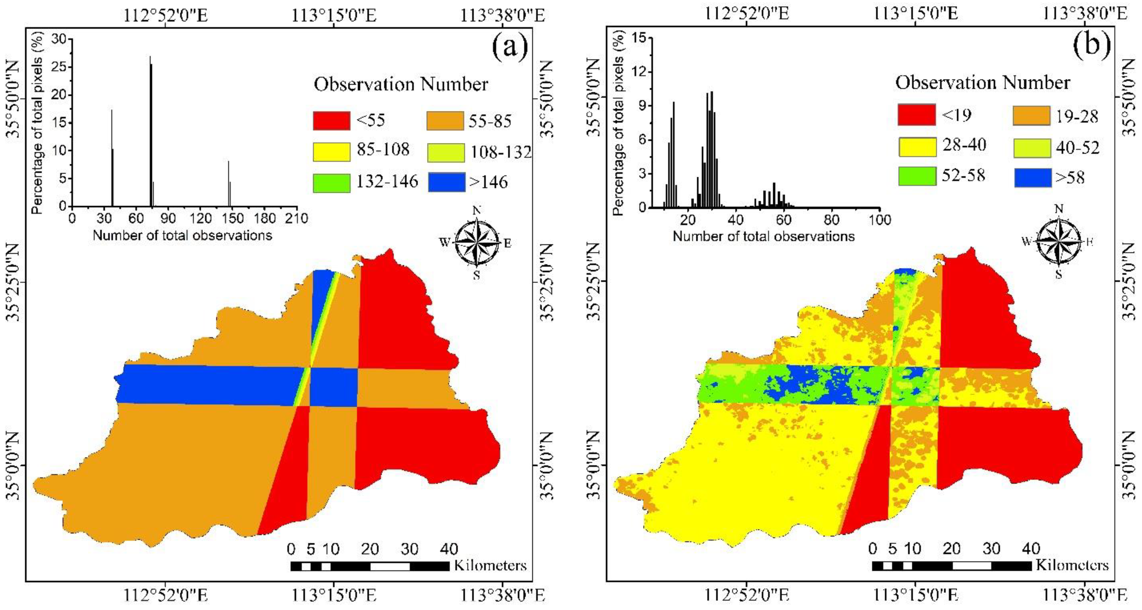
Sentinel-2 consists of two satellites, launched in June 2015 (Sentinel-2A) and March 2017 (Sentinel-2B), with a revisit period of 5 days. The Sentinel-2 sensor has a total of 13 spectral bands including visible light, near-infrared, and short-wave infrared; this study used bands 2–4 and band 8 (with spatial resolution of 10 m), as well as bands 5–7 and bands 11–12 (with a spatial resolution of 20 m). A total of 263 Sentinel-2 (Level-1C) images were used as the optical data for this study (Figure 2a). To remove cloud and cloud shadows, the C Function of Mask (CFMask) algorithm was used, and the result of “de-cloud processing” is shown in Figure 2b. Then, bands 5–7 and bands 11–12 were resampled to 10 m. To generate high-quality composites, we used a 10 day synthesis method to improve the accuracy of the phenological period of crops [36]. For synthesized images that did not cover the entire study area, we used the median value of images captured 10 days before and after for interpolation. Lastly, the monthly median values of bands 2–8 and bands 11–12 were calculated.

Three VI_S, namely, the NDVI, land surface water index (LSWI), and EVI, were also used as complementary layers for each Sentinel-2 image. The NDVI can monitor the growth of crops very well [37]. The EVI is an “optimized” VI with greater sensitivity in areas with high crop variety [38]. The LSWI is sensitive to the total amount of liquid water in vegetation [39]. The equations used to calculate these derived indices are as follows [40,41,42]:

$$\mathrm{NDVI}=\frac{\mathrm{NIR} - \mathrm{RED}}{\mathrm{NIR} + \mathrm{RED}}$$

(1)

$$\mathrm{EVI}=2.5\times \frac{\mathrm{NIR} - \mathrm{RED}}{\mathrm{NIR} +6\times \mathrm{RED} -7.5\times \mathrm{BLUE} +1}$$

(2)

$$\mathrm{LSWI}=\frac{\mathrm{NIR} - \mathrm{SWIR}}{\mathrm{NIR} + \mathrm{SWIR}}$$

(3)

We used the Savitzky–Golay (S–G) algorithm to reconstruct the time series VI and spectral bands because, although the original timeseries VI and spectral bands use an interpolation algorithm, there is still noise [43].

2.2.2. Sentinel-1 Imagery

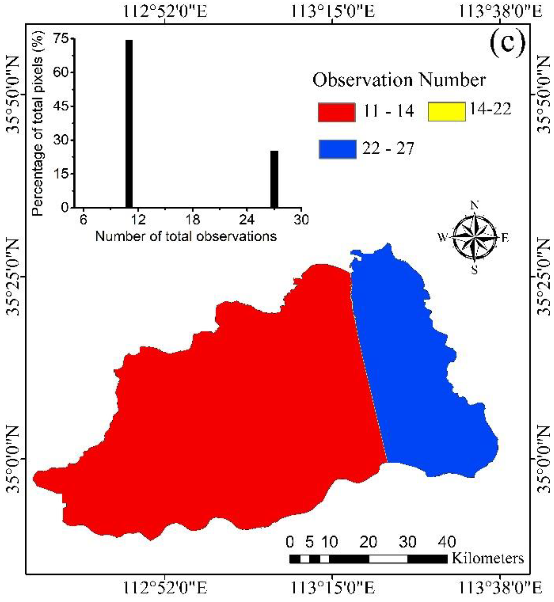
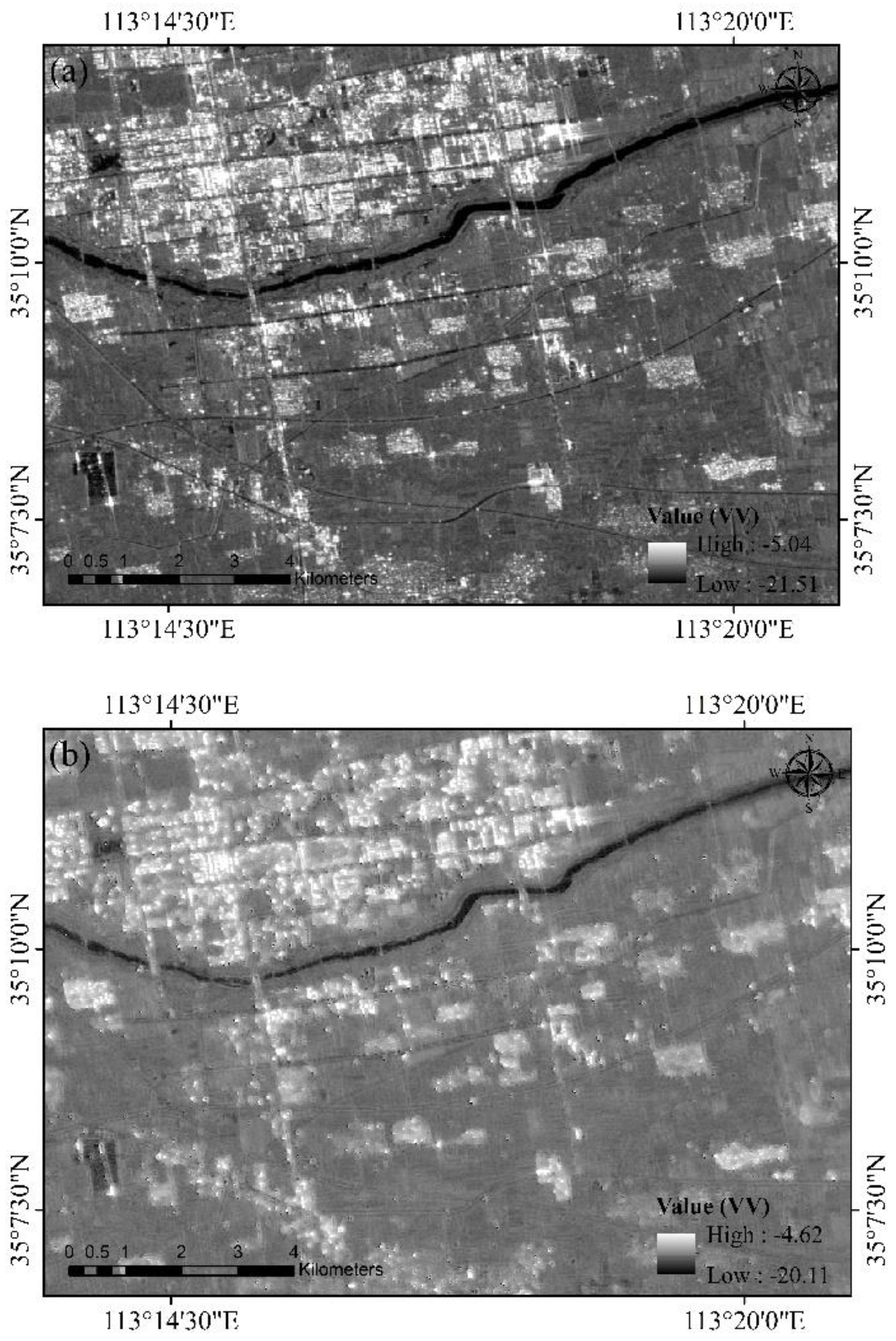
Sentinel-1 is a SAR system with a 12 day revisit period and a spatial resolution of 10 m. The satellite acquires C-band data in dual polarization, ascent, and descent modes. Sentinel-1 data were used in this study because some studies have reported that SAR data can improve crop classification and depict crop phenology with high accuracy [31,44]. A total of 26 scenes of Sentinel-1 images were acquired during the summer crop growth period using the GEE (Figure 2c). All of the Sentinel-1 images were preprocessed by the Sentinel-1 toolbox, including thermal noise removal, radiometric scaling, and terrain correction. However, Sentinel-1 data were also affected by speckle noise, which randomly appeared in the images [45]. The Lee filter algorithm was then used to remove this noise in this study (Figure 3) [46]. In addition to the selection of vertical transmit/vertical receive (VV) and vertical transmit/horizontal receive (VH) polarization bands, we calculated six texture features of the VV and VH polarization bands through the gray-level cooccurrence matrix (GLCM), namely, angular second moment, contrast, correlation, variance, inverse differential moment, and sum average [47]. However, through the feature importance ranking results, we found that the texture features of the VV and VH polarization bands had little influence on the crop classification results; thus, we removed the texture features of VV and VH polarization bands in this study.

2.2.3. Ground Reference Dataset

A total of 763 sample points were collected in 2021, including water (33 points), impervious surface (102 points), forest (60 points), grassland (44 points), maize (222 points), peanut (120 points), soybean (60 points), yam (45 points), cotton (46 points), and other crops (31 points) (Figure 1b). In the field survey, we obtained the coordinates of the type of crop land through real-time kinematics (RTK), a measuring instrument capable of obtaining centimeter-level positioning accuracy in real time in the field. Most of the field points were collected in areas of uniform land use, which were longer than 20 m in each direction. To ensure consistency between the reference data and imagery, we set the buffer distance for each training sample to 10 m [14]. To avoid classification overfitting, we randomly divided all samples into training samples (about 60%) and validation samples (about 40%). We also generated buffer polygons for the validation samples of each crop type based on field survey data and Google Earth images, and we finally collected 27 polygons (11,254 pixels) for the maize, 20 polygons (9119 pixels) for the peanut, 12 polygons (1700 pixels) for the yam, 15 polygons (4903 pixels) for the soybean, four polygons (397 pixels) for the cotton, and four polygons (206 pixels) for the other crops as validation samples. These polygonal buffers were superimposed with the Google Earth high resolution images, and the crop type validation grids were obtained through visual interpretation. We also obtained city- and county-level statistics from the Jiaozuo City Statistical Yearbooks in 2019 and 2020 for comparison with the results obtained in this study. The data are available at: https://tjj.jiaozuo.gov.cn/template, accessed on 13 June 2022.

2.2.4. Land-Cover Map in 2020

A 30 m land-cover map of China for 2020 (LCM30) was acquired from the Global Geoinformation Public Product (GlobeLand30; http://www.globallandcover.com/, accessed on 18 May 2022). The LCM30 was generated using Landsat images and 16 m spatial resolution High Fraction 1 (GF-1) multispectral images from 2020, with an overall accuracy (OA) of 85.72% and kappa coefficient (KC) of 0.82. In the LCM30 map, there were 10 primary land use land cover (LULC) types (cropland, grassland, forest, urban areas, etc., details of which can be found in [48]). However, the classification system of the map did not include a crop type layer. We compared the land-cover map generated in this study with the LCM30 map.

2.3. Methods

2.3.1. Crop Type Mapping Algorithms

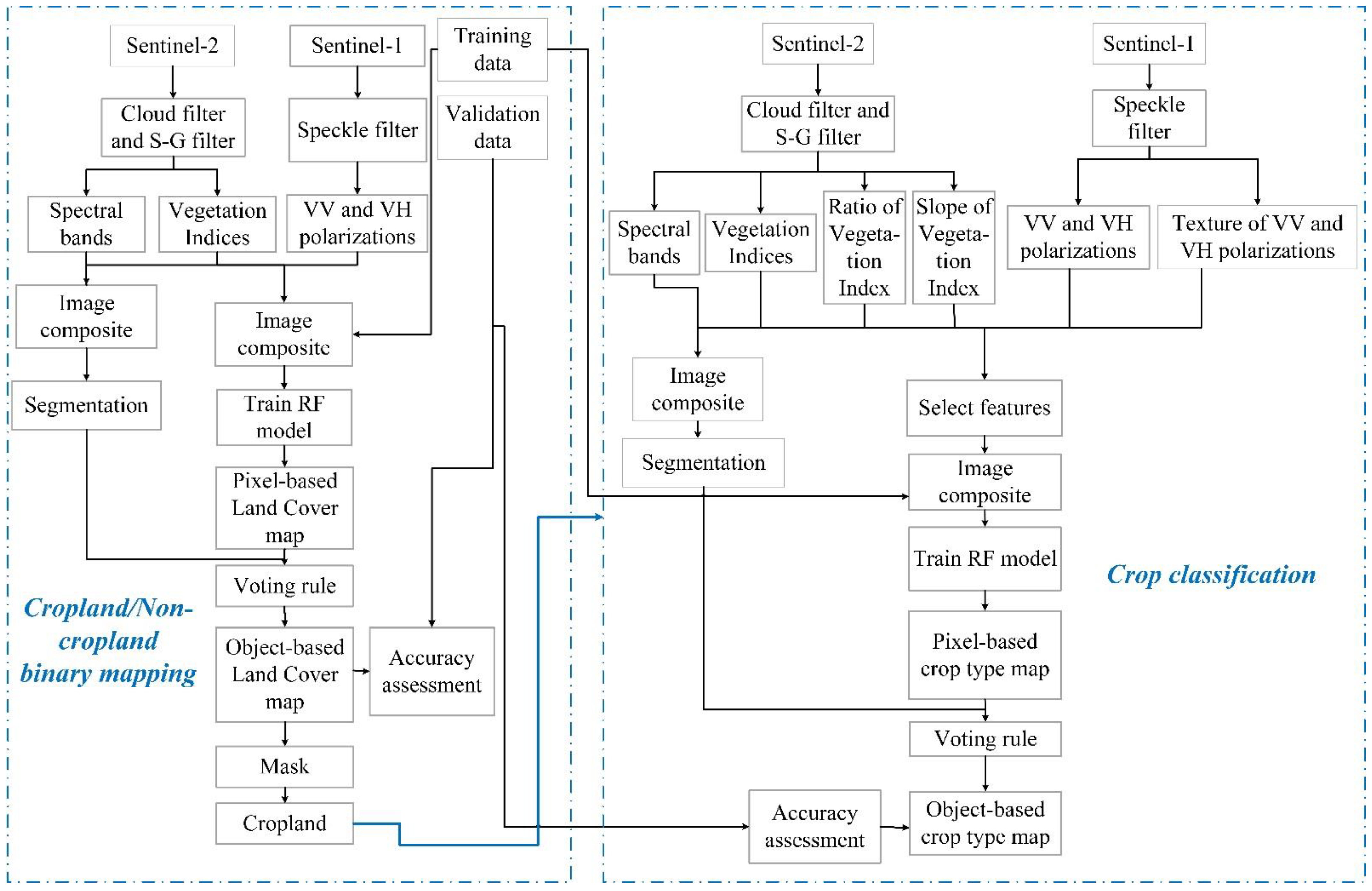
We developed a combination of object-based and pixel-based mapping algorithm for summer crop type maps (Figure 4). The algorithm was divided into two parts for each pixel: (1) identification of the primary land-cover map for cropland masks, and (2) classification of the type of crop land (based on introducing phenological characteristics at critical stages).

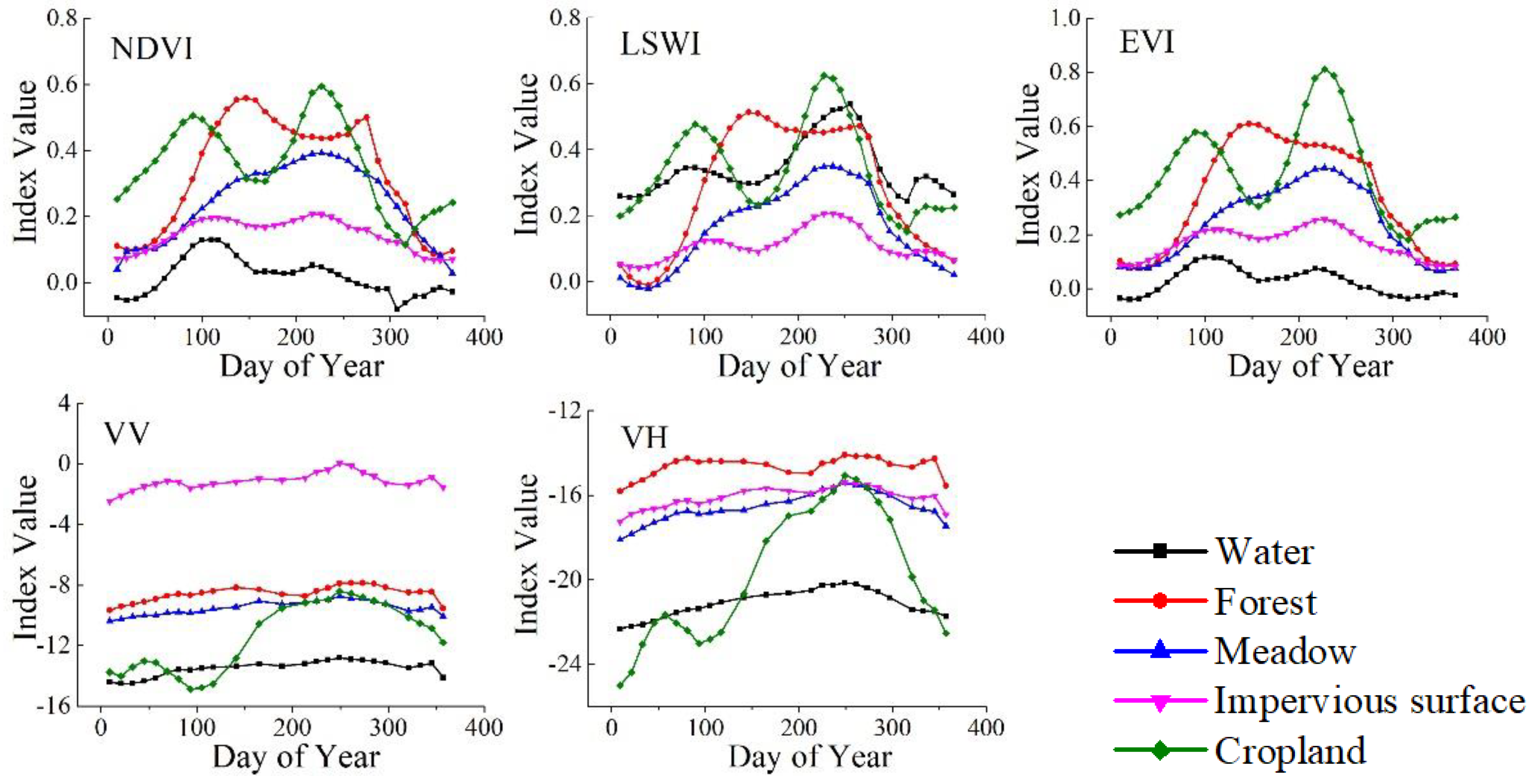
The time series curves of the VI, VV, and VH polarization bands were very different between cropland and non-cropland (Figure 5). Ghorbanian et al. successfully distinguished land-cover types on the basis of synthetic aperture radar (SAR) imagery and monthly median values of common vegetation indices for Iran [30]. Huang et al. used time series NDVI and spectral bands to draw a land-cover map of Beijing based on Landsat images [49]. To avoid interference from non-cropland areas (e.g., meadow, forest, water, and urban areas), we first classified primary land cover into five types to obtain the cropland layer. We constructed a feature set including the monthly median values of VV and VH polarization bands in Sentinel-1 data, the monthly median values of bands 2–8 and 11–12 in Sentinel-2 data, and the monthly median values of EVI, LSWI, and NDVI. A pixel-based land-cover map (LCM) was generated on the basis of this feature set and RF method. To avoid the noise associated with pixel-based classification, we combined object segmentation and pixel-based classification to improve the accuracy and remove “speckle” noise [22,31]. The simple noniterative clustering (SNIC) image segmentation method of the GEE platform was used to segment the cloud-free Sentinel-2 data, and the segmentation results were combined with the results of a pixel-based classification. An important parameter of the SNIC function is the seed, the size of which directly affects the results of object segmentation. Through multiple simulations, for areas with a single feature type, such as land types with only forests or buildings, the seed value was set to 50, and, in areas where cropland and other land types coexist, we set the seed value to 30. On the basis of the pixel-based classification results, the area of each primary land-cover type within each segmented object was calculated. The category of each object was that of the land-cover type with the largest area within the object. Then, a cropland/non-cropland binary map was generated, and the satellite data were finally masked by the cropland layer.

The RF is reportedly the most stable and accurate classifier for crop land mapping across different agricultural systems, which is very popular in the field of remote sensing [50,51,52]. The RF is an ensemble classifier that contains a number of decision trees, where the optimal classification result is voted on the basis of the classification results of each decision tree [53]. The number of trees is a key parameter for classification. In this study, we selected the number of trees in each classifier by simulating the classification accuracy according to the number of trees. Lastly, the number of trees for the classifier used to generate the LCM was set to 80, and the number of trees for crop type classification was set to 65. In addition, to ensure stability and accuracy of classification, we used the “explain” function of the GEE platform to determine the importance of all features, sorted the features according to their importance, and used the sorted results as a feature set for training [11].

Furthermore, as can be seen in Figure 6, there were special spectral characteristics at the beginning and end of the growing season, although the time series curves of the NDVI, EVI, and LSWI for the different crop types had many similarities during the whole growth period. To highlight the discriminative features at some specific and key points on the time series profile, two phenological indices at key growth stages, namely, slope of vegetation index change (VI_slope) and relative change ratio of vegetation index (VI_ratio), were developed. Definitions of the index formulas used are as follows:

$${\mathrm{NDVI}}_{\mathrm{slope}}=100\times \frac{{\mathrm{NDVI}}_{\mathrm{i}+1}-{ \mathrm{NDVI}}_{\mathrm{i}}}{{\mathrm{DAY}}_{\mathrm{i}+1}-{ \mathrm{DAY}}_{\mathrm{i}}}$$

(4)

$${\mathrm{EVI}}_{\mathrm{slope}}=100\times \frac{{\mathrm{EVI}}_{\mathrm{i}+1}-{ \mathrm{EVI}}_{\mathrm{i}}}{{\mathrm{DAY}}_{\mathrm{i}+1}-{ \mathrm{DAY}}_{\mathrm{i}}}$$

(5)

$${\mathrm{LSWI}}_{\mathrm{slope}}=100\times \frac{{\mathrm{LSWI}}_{\mathrm{i}+1}-{ \mathrm{LSWI}}_{\mathrm{i}}}{{\mathrm{DAY}}_{\mathrm{i}+1}-{ \mathrm{DAY}}_{\mathrm{i}}},$$

(6)

$${\mathrm{NDVI}}_{\mathrm{ratio}}=\frac{\mathrm{NDVI} -{ \mathrm{NDVI}}_{\max }}{{\mathrm{NDVI}}_{\max }-{ \mathrm{NDVI}}_{\min }}$$

(7)

$${\mathrm{EVI}}_{\mathrm{ratio}}=\frac{\mathrm{EVI} -{ \mathrm{EVI}}_{\max }}{{\mathrm{EVI}}_{\max }-{ \mathrm{EVI}}_{\min }}$$

(8)

$${\mathrm{LSWI}}_{\mathrm{ratio}}=\frac{\mathrm{LSWI} -{ \mathrm{LSWI}}_{\max }}{{\mathrm{LSWI}}_{\max }-{ \mathrm{LSWI}}_{\min }}$$

(9)

where ${\mathrm{VI}}_{\mathrm{i}}$ is the value of the VI on the i-th day, ${\mathrm{VI}}_{\mathrm{imin}}$ is the minimum value of VI during key growth stages, and ${\mathrm{VI}}_{\max }$ is the maximum value of VI during key growth stages.

Moreover, an excessive number of input features may affect the classification results [54] and the efficiency of the GEE platform. Therefore, the monthly median values of VI, VI_slope, and VI_ratio at the key growth stages of the growing season (June and October) were proposed for crop classification (colored frame in Figure 6). To evaluate the advantages of the proposed new indices and assumption, five schemes were developed as follows:

Scheme 1: the monthly median values of the VV and VH polarization bands and bands 2–8 and 11–12, as well as the EVI, NDVI, and LSWI during the crop growing period, were used for classification.

Scheme 2: the monthly median values of the VV and VH polarization bands and bands 2–8 and 11–12, as well as the EVI, NDVI, and LSWI during the key growth stages, were used for classification.

Scheme 3: on the basis of scheme 2, VI_slope was added at key growth stages for classification.

Scheme 4: on the basis of scheme 2, VI_ratio was added at key growth stages for classification.

Scheme 5: on the basis of scheme 2, both VI_slope and VI_ratio were added at key growth stages for classification.

Meanwhile, to reduce confusion among different crops, the pixel-based crop classification results were combined with image segmentation to create clear crop distribution map. For areas with complex crop types, we set the seed value to 10.

2.3.2. Accuracy Assessment

Generally, OA and KC are used to evaluate classification results, but the KC value may be contingent, and it is difficult to reflect the classification accuracy [55]; hence, in addition to OA and KC, we also calculated producer’s accuracy (PA), user’s accuracy (UA), and F1-score to evaluate the accuracy of classification. The F1-score is a metric for measuring the agreement between classified and reference samples; the F1-score is defined as follows [56]:

$$\mathrm{F}1-\mathrm{Score}=2\times \frac{\mathrm{UA}\times \mathrm{PA}}{\mathrm{UA} +\mathrm{PA}}$$

(10)

For a more comprehensive visual interpretation, we compared our results with the LCM30 and high-resolution Google Earth images in four subsets for cropland mask assessment. Additionally, the type of crop land was further compared with high-resolution Google Earth images in three other subsets.

3. Results

3.1. Annual Map of Land-Cover Types in 2021

Figure 7 and

Table 1. Classification accuracy for primary land cover over Jiaozuo City based on pixel- and object-based mapping algorithms.

Class	Error Matrix				Accuracy (%)
	Crop	Forest	Meadow	Impervious Surface	Water	Producer’s	User’s	F1-Score	OA
Crop	209	0	0	3	0	98.56	98.56	98.56	95.42
Forest	0	19	3	1	0	78.95	84.21	81.50
Meadow	1	3	13	0	0	69.23	69.23	69.23
Impervious Surface	1	0	1	39	0	94.87	89.74	92.23
Water	1	0	0	0	12	91.67	100.00	95.65

show the primary land-cover classification accuracy. According to the primary land-cover classification results, the OA and KC values were 95.42% and 0.89, respectively. Specifically, meadow was the main class incorrectly mixed with other land-cover types, with PA, UA, and F1-Score < 80%. This may be partly due to the confusion between forest and meadow, with about 17.65% of the meadow test sample points being misclassified as forest and 17.39% of the forest test sample points being misclassified as meadow. Meadows were also easily confused with green belts in built-up areas, with about 2.44% of urban test samples being misclassified as meadows. Due to the relatively distinct spectral features and temporal patterns of cropland with other primary land-cover types, the PA, UA, and F1-scores of cropland appeared higher than 98%.

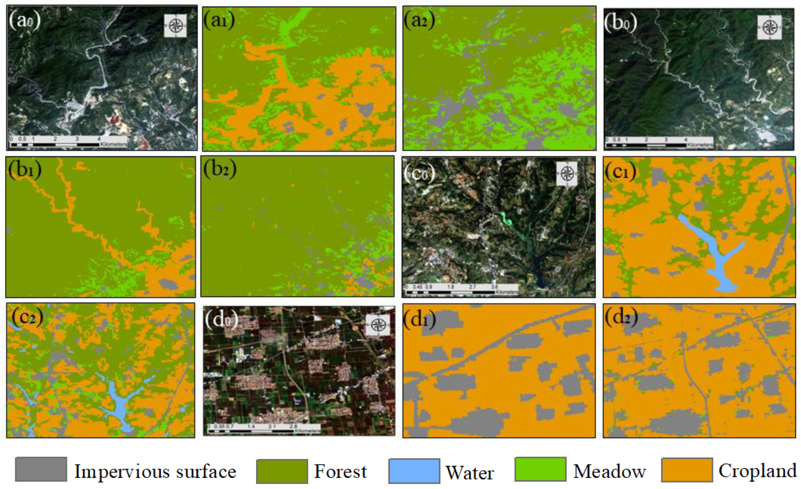
It can be clearly observed that there was a significant improvement in the primary land cover using the proposed methodology, although the spatial pattern of these land-cover types was generally consistent with LCM30 (Figure 7 and Figure 8). For instance, the proposed methodology successfully delineated impervious surfaces and meadow classes (Figure 8a₀–a₂), while these classes were mostly misclassified as cropland in LCM30, which could be due to the coarse spatial resolution of LCM30 and single optical image sources. The proposed methodology also discriminated the forest and accurately classified the southeast region into forest, meadow, and cropland classes (Figure 8b₀–b₂). In addition, it is evident from Figure 8c₀–c₂ that the water class was better classified using the proposed method compared to LCM30. Furthermore, the proposed approach was capable of correctly delineating the area covered by cropland and green belt in the rural–urban–cropland ecotone (Figure 8d₀–d₂). These results indicate that the proposed methodology may be satisfactory for cropland masking.

3.2. Annual Map of Major Crop Types in 2021

Table 2. Crop type classification accuracy of different schemes based on the pixel- and object-based mapping algorithm.

Cropland	Scheme 1			Scheme 2			Scheme 3			Scheme 4			Scheme 5
	Producer’s (%)	User’s (%)	F1-Sore (%)	Producer’s (%)	User’s (%)	F1-Sore (%)	Producer’s (%)	User’s (%)	F1-Score (%)	Producer’s (%)	User’s (%)	F1-Score (%)	Producer’s (%)	User’s (%)	F1-Score (%)
Maize	99.09	93.27	96.09	98.01	93.87	95.90	98.98	88.31	93.34	98.94	93.22	95.99	98.98	93.27	96.04
Peanut	93.79	87.31	90.43	93.64	90.33	91.96	90.85	95.55	93.15	92.64	87.92	90.22	90.56	96.54	93.45
Yam	61.82	87.51	72.46	61.00	87.14	71.76	83.64	88.87	86.18	77.47	81.95	79.65	85.35	87.25	86.29
Other	100	96.74	98.34	84.13	100	91.38	100	91.22	95.41	100	91.63	95.63	99.04	88.40	93.42
Soybean	68.12	83.79	75.15	75.28	87.31	80.85	79.62	93.11	85.84	67.32	89.21	76.73	81.19	93.36	86.85
Cotton	100	92.78	96.25	100	85.40	92.13	100	91.02	95.30	100	80.04	88.91	100	87.54	93.36
OA (%)	89.55			90.64			91.92			89.93			93.22
KC	0.84			0.87			0.88			0.85			0.89

shows the change in crop type classification accuracy for the different schemes. As shown in Table 2, the classification accuracy of scheme 2 was higher than that of scheme 1, indicating that introducing common vegetation indices at the beginning and end of the growing season and reducing common vegetation indices during other periods improved the crop type classification accuracy. The scheme including VI_slope at the critical period achieved an OA of 91.92% and KC of 0.88 for the crop type classification, and it was superior to scheme 2. Thus, adding the VI_slope at the critical period for crop type classification could be beneficial for classification accuracy. In comparison, adding the VI_ratio at the critical period on the basis of scheme 2 did not improve the overall classification accuracy much (scheme 4), but greatly improved the classification accuracy for yam, which suggested that the VI_ratio at the critical period was more useful for low-stem crop classification. Overall, scheme 5 including both VI_ratio and VI_slope in the critical period of crop growth yielded the best classification performance, with an OA of 93.22% and KC of 0.89. Scheme 5 also achieved a larger PA, UA, and F1-score for each crop type map. This finding indicates the importance of combining VI_ratio and VI_slope in the critical period for crop type classification.

To make the results of this classification more obvious, four image subsets corresponding high-resolution Google Earth images were produced (Figure 9). It can be seen from Figure 9 that the results of scheme 5 were roughly consistent with the field survey and high-resolution Google Earth images. For example, it successfully delineated cotton, maize, and peanut points, and it distinguished the cotton boundary more clearly (Figure 9a₅), whereas schemes 1–4 had more broken areas for cotton and peanut regions (Figure 9a₁–a₄). Moreover, soybean and yam patches were also clearly identified in Figure 9b₅,d₅ under scheme 5. However, some parts of the peanuts and soybeans were confused (Figure 9b₅), which could be partly attributed to the similar growth features, but also to the smaller size of the seed points set for areas with complex crop types when we performed image segmentation.

3.3. Comparison of Crop Area Estimates from the Remote Sensing Approach and Agricultural Statistical Reports

As shown in Figure 9A, the total area of cropland in Jiaozuo determined by this study was 1735.25 km², which was 14.50% less than the area estimated from agricultural statistics reported in 2019 (2030.65 km²) and 10.73% less than the area estimate reported in 2018 (1943.92 km²). This difference was probably related to the fact that the plastic greenhouses were not considered in this study. Additionally, as the largest distributions of the three main crops in Jiaozuo City, maize was widely planted in the piedmont plain, with a total area from this study of 1380.87 km², which was about 177.92 km² higher than the average area from the 2019 and 2020 statistical yearbooks (Figure 10). In the study area, farmland shelterbelt and country lanes were widely distributed around cropland, with both likely to be divided into the main crop fields at 10 m resolution (which would have resulted in overestimation of the planting area). In comparison, soybean was distributed mainly over Wuzhi and Qinyang counties, with a total area almost equal to that of the average statistical data. For peanut, although the proposed methodology successfully captured its main distribution region, the statistical results showed that its planting area was slightly larger than that derived in this study, partly attributable to a submerged farm field near the Yellow River Beach that formed following a rainstorm in July 2021 (Figure 9A and Figure 10).

4. Discussion

4.1. Potential Applications of SAR and Optical Images for Crop Type Mapping

Smallholder farming has long been the dominant practice in China’s agricultural system. The small size of the cropland area has resulted in a mixture of different crop types due to the limitations of the spatial resolution of moderate optical images [57]. Although Landsat provides high-spatial-resolution images, it may not provide high-quality data during the summer because of its low temporal resolution and cloud influence. In comparison, SAR has high penetrating power and no cloud interference. It can be, therefore, used to monitor the real growth of vegetation [58,59]. The integration of SAR data with these optical images provides an effective solution to the problems of low availability of high-quality data and low spatial resolution of the crop type classification in regions with small plots.

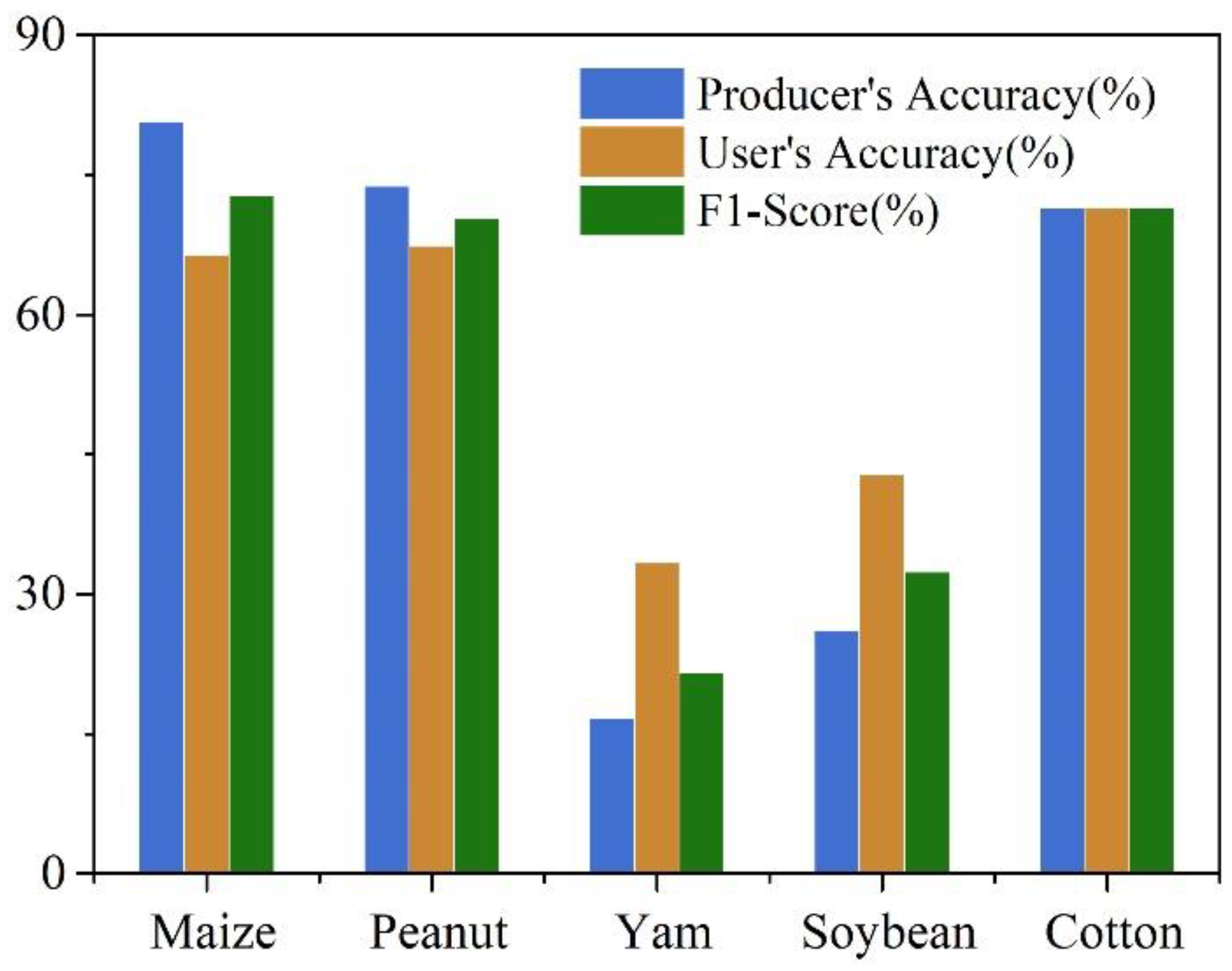
We compared crop type classification accuracy on the basis of only SAR data from Sentinel-1, optical data from Sentinel-2, and the integration of SAR and optical data, according to the schemes used for crop type classification (

Table 3. Accuracy of crop type determinations based only on the SAR data from Sentinel-1, optical data from Sentinel-2, and integration of SAR and Sentinel-2 data.

Scheme	Optical Data		SAR Data		SAR and Optical Data
	OA (%)	KC	OA (%)	KC	OA (%)	KC
Scheme 1	86.57	0.81	65.15	0.48	89.55	0.84
Scheme 2	89.20	0.85			90.64	0.87
Scheme 3	90.33	0.86			91.92	0.88
Scheme 4	89.84	0.85			89.93	0.85
Scheme 5	90.76	0.86			93.22	0.89

). The crop type distribution maps generated by the integration of SAR and Sentinel-2 data generally had higher OA and KC values, whereas those generated only from SAR data had lower OA and KC values. As with previous studies, although the use of SAR data had some advantages for all-weather monitoring, the classification results based only on SAR data seemed to be worse than that with spectral features, with an OAs of about 58–65% [60] and 35–65% [61], respectively. Adding SAR images to supplement the optical images improved the accuracy of crop classification by approximately 5% [61]. These results not only indicated the key contribution of the optical data in crop classification, but also suggested that SAR images combined with the optical image data could indeed improve crop discrimination. In addition, land-cover types probably had unique sensitivity to SAR (Figure 11), as evidenced by the F1-score of 72.73% for maize, which is consistent with the result of You et al. [16], and 21.55% for yam, indicating that the improved efficiency of the crop identification by combining SAR images differed according to crop type.

4.2. Algorithm Improvement

Previous studies have demonstrated the feasibility of classifying crops on the basis of phenological stages [62]. For example, Belgiu et al. successfully identified multiple crops in three different regions on the basis of images of crops in each phenological period [63]. However, for areas with a wide variety of crops, the phenomenon that we refer to as “different cropland with the same spectrum” still occurred in some phenological periods, which may have led to erroneous results [64]. For example, the EVI time series curves of maize and soybean were very similar in the crop growth period (Figure 6). Therefore, it was difficult to identify the crop category using only the common VI temporal profile, in addition to the confusion of forests and grasslands with cropland [54].

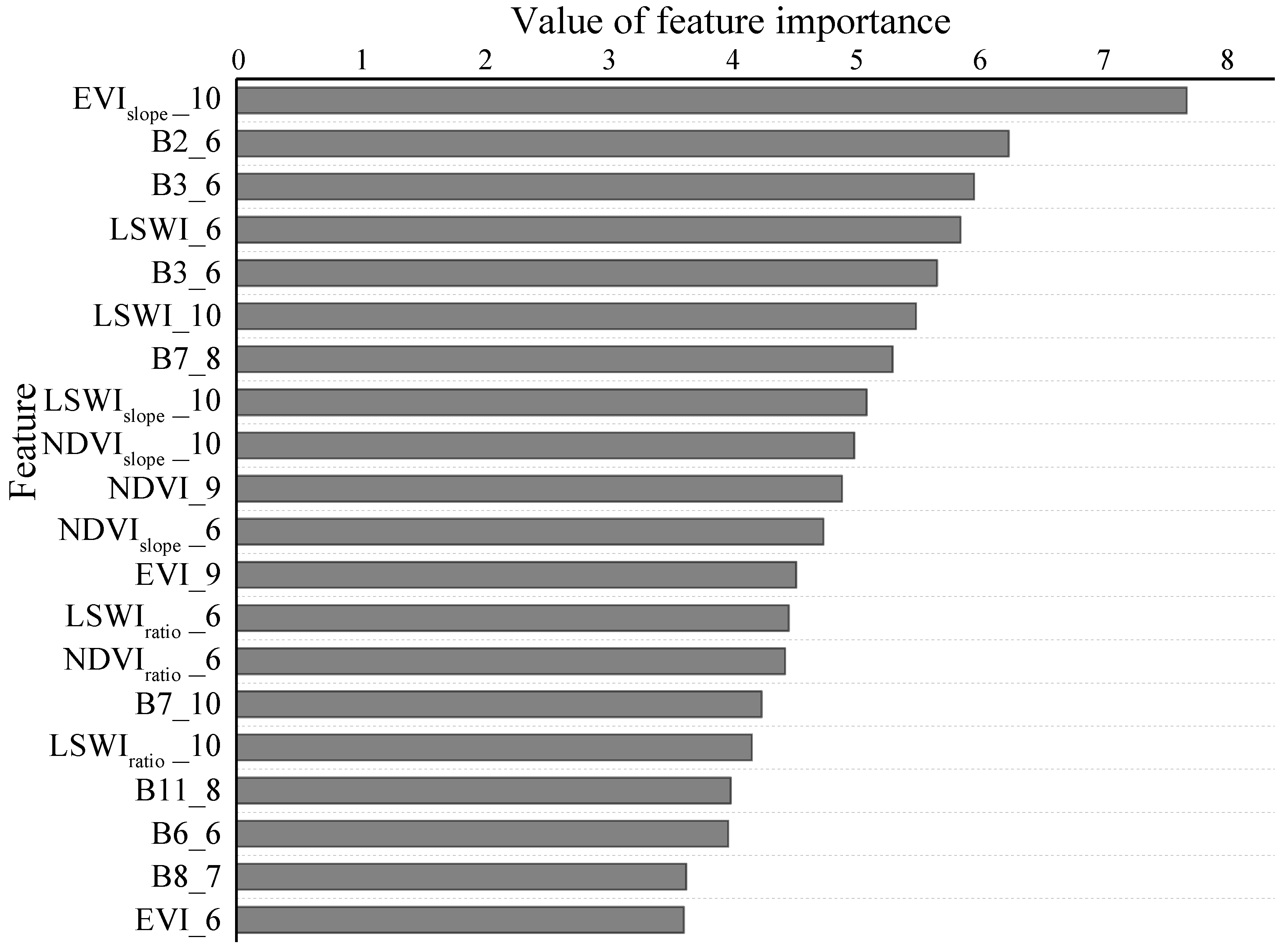
To address these issues, we first created an LCM of Jiaozuo City on the basis of optical and SAR data to generate a cropland mask, using the RF classification method. After that, considering the classification advantages based on crop phenological cycles and crop growth characteristics at the key growth stages, we developed two new indices, VI_slope and VI_ratio, as a function of the crop growth rate, to improve the classification accuracy. Meanwhile, previous studies pointed out that an excessive number of features may affect the classification results [65], and the purpose of the feature selection should be to eliminate unimportant and redundant features [66]. We then analyzed the importance of each feature for classification using the GEE platform’s explain method and also found that the VI_slope, VI_ratio, and median values of VI of the sowing and harvesting periods were relatively important (Figure 12). When the five schemes were compared, the results showed that the highest accuracy was obtained when both VI_slope and VI_ratio in the critical period of crop growth were added to the feature set (Table 2). This could be partly attributed to the fact that different types of crops exhibited different growth rates under the same time period, and they could also be associated with a reduction in information redundancy.

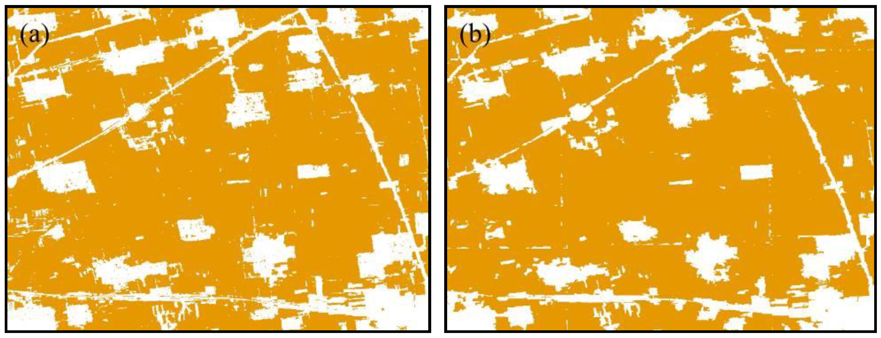
Image segmentation divided pixels with the same criteria into one object [67], which alleviated the problem of salt-and-pepper noise. In most cases, object-based classification results were better than pixel-based ones [68,69]. We used the SNIC method for segmentation of Sentinel-2 synthetic images during the crop growth period, and then combined the segmentation results with the pixel-based classification results to obtain high classification accuracy (Figure 13).

4.3. Uncertainty

Our results showed that the proposed methodology was able to identify crop categories, but there were still some uncertainties. First, we used larger-sized seed parameters for regions with a single crop species than for regions with a complex pattern of species (Figure 14). To avoid crop misclassification, the size of the seed segmentation parameters was set to be small for areas with a variety of crops, which led to over-segmentation for some objects. The optimal segmentation parameters for crop segmentation should be further explored. Second, the number and quality of images can affect the classification results. A total of 236 Sentinel-2 images were collected for crop classification in this study (average of 73.08 revisits per pixel); however, after removing clouds and cloud shadows, the average number of revisits per pixel decreased to 27.9. The lack of high-quality observed images made it limited to capture crucial information about crop growth, which affected the classification results. In addition, more validation samples based on field surveys and appropriate sample proportion are needed for accurate quality assessment, and major efforts are still required for ground truth sample collection in the future. A recent study suggested that the migration model can classify crops for different years using the same set of samples [70], which could be developed to systematically track and monitor the dynamics of crop type distribution.

5. Conclusions

In this study, a combined object- and pixel-based mapping workflow for 10 m resolution crop type mapping by combining time series optical images (Sentinel-2) and synthetic aperture radar images (Sentinel-1) based on the Google Earth Engine platform was proposed. Firstly, we identified five primary land-cover types by using the Sentinel-1 and Sentinel-2 monthly composite images combined with the RF classifier, and then masked non-cropland to generate a cropland and non-cropland binary map. Secondly, we developed two new indices, namely, VI_slope and VI_ratio, and we generated a crop type distribution on the cropland map formed above by comparing the classification accuracy of five schemes. The scheme when VI_ratio and VI_slope were added during the critical period of crop growth showed the best classification performance, with a total OA of 93.22% and KC of 0.89, as well as relatively larger PA, UA, and F1-score for each crop type map, suggesting that the VI_slope and VI_ratio indices at the critical period have potential for mapping crop types in smallholder farming regions. In addition, our results highlighted that, although the median values of the VV and VH bands were insensitive to crop type mapping, adding this information to supplement optical images would be helpful for improving the accuracy of crop type classification.

References

1. Du, Y.; Xu, Y.; Zhang, L.; Song, S. Can China’s food production capability meet her peak food demand in the future? Int. Food Agribus. Man. 2020, 23, 1–18. [Google Scholar] [CrossRef]
2. Sheng, Y.; Song, L. Agricultural production and food consumption in China: A long-term projection. China Econ. Rev. 2019, 53, 15–29. [Google Scholar] [CrossRef]
3. Ning, J.; Liu, J.; Kuang, W.; Xu, X.; Zhang, S.; Yan, C.; Li, R.; Wu, S.; Hu, Y.; Du, G. Spatiotemporal patterns and characteristics of land-use change in China during 2010–2015. J. Geogr. Sci. 2018, 28, 547–562. [Google Scholar] [CrossRef] [Green Version]
4. Yu, Q.; Hu, Q.; van Vliet, J.; Verburg, P.H.; Wu, W. GlobeLand30 shows little cropland area loss but greater fragmentation in China. Int. J. Appl. Earth Obs. Geoinf. 2018, 66, 37–45. [Google Scholar] [CrossRef]
5. Arino, O.; Gross, D.; Ranera, F.; Leroy, M.; Bicheron, P.; Brockman, C.; Defourny, P.; Vancutsem, C.; Achard, F.; Durieux, L. GlobCover: ESA service for global land cover from MERIS. In Proceedings of the 2007 IEEE International Geoscience and Remote Sensing Symposium, Barcelona, Spain, 23–28 July 2007. [Google Scholar]
6. Friedl, M.A.; McIver, D.K.; Hodges, J.C.; Zhang, X.Y.; Muchoney, D.; Strahler, A.H.; Woodcock, C.E.; Gopal, S.; Schneider, A.; Cooper, A. Global land cover mapping from MODIS: Algorithms and early results. Remote Sens. Environ. 2002, 83, 287–302. [Google Scholar] [CrossRef]
7. Hu, Q.; Xiang, M.; Chen, D.; Zhou, J.; Wu, W.; Song, Q. Global cropland intensification surpassed expansion between 2000 and 2010: A spatio-temporal analysis based on GlobeLand30. Sci. Total Environ. 2020, 746, 141035. [Google Scholar] [CrossRef]
8. Boryan, C.; Yang, Z.; Mueller, R.; Craig, M. Monitoring US agriculture: The US department of agriculture, national agricultural statistics service, cropland data layer program. Geocarto Int. 2011, 26, 341–358. [Google Scholar] [CrossRef]
9. Fisette, T.; Rollin, P.; Aly, Z.; Campbell, L.; Daneshfar, B.; Filyer, P.; Smith, A.; Davidson, A.; Shang, J.; Jarvis, I. AAFC annual crop inventory. In Proceedings of the 2013 Second International Conference on Agro-Geoinformatics (Agro-Geoinformatics), Fairfax, VA, USA, 12–16 August 2013. [Google Scholar]
10. Ghassemi, B.; Dujakovic, A.; Żółtak, M.; Immitzer, M.; Atzberger, C.; Vuolo, F. Designing a European-Wide Crop Type Mapping Approach Based on Machine Learning Algorithms Using LUCAS Field Survey and Sentinel-2 Data. Remote Sens. 2022, 14, 541. [Google Scholar] [CrossRef]
11. Chong, L.; Liu, H.; Lu, L.; Liu, Z.; Kong, F.; Zhang, X. Monthly composites from Sentinel-1 and Sentinel-2 images for regional major crop mapping with Google Earth Engine. J. Integr. Agric. 2021, 20, 1944–1957. [Google Scholar] [CrossRef]
12. Vuolo, F.; Neuwirth, M.; Immitzer, M.; Atzberger, C.; Ng, W. How much does multi-temporal Sentinel-2 data improve crop type classification? Int. J. Appl. Earth Obs. Geoinf. 2018, 72, 122–130. [Google Scholar] [CrossRef]
13. Ni, R.; Tian, J.; Li, X.; Yin, D.; Li, J.; Gong, H.; Zhang, J.; Zhu, H.; Wu, D. An enhanced pixel-based phenological feature for accurate paddy rice mapping with Sentinel-2 imagery in Google Earth Engine. ISPRS J. Photogramm. Remote Sens. 2021, 178, 282–296. [Google Scholar] [CrossRef]
14. Zurqani, H.A.; Post, C.J.; Mikhailova, E.A.; Schlautman, M.A.; Sharp, J.L. Geospatial analysis of land use change in the Savannah River Basin using Google Earth Engine. Int. J. Appl. Earth Obs. Geoinf. 2018, 69, 175–185. [Google Scholar] [CrossRef]
15. Adrian, J.; Sagan, V.; Maimaitijiang, M. Sentinel SAR-optical fusion for crop type mapping using deep learning and Google Earth Engine. ISPRS J. Photogramm. Remote Sens. 2021, 175, 215–235. [Google Scholar] [CrossRef]
16. You, N.; Dong, J. Examining earliest identifiable timing of crops using all available Sentinel 1/2 imagery and Google Earth Engine. ISPRS J. Photogramm. Remote Sens. 2020, 161, 109–123. [Google Scholar] [CrossRef]
17. Sujud, L.; Jaafar, H.; Hassan, M.A.H.; Zurayk, R. Cannabis detection from optical and RADAR data fusion: A comparative analysis of the SMILE machine learning algorithms in Google Earth Engine. Remote Sens. Appl. 2021, 24, 100639. [Google Scholar] [CrossRef]
18. Ma, Z.; Liu, Z.; Zhao, Y.; Zhang, L.; Liu, D.; Ren, T.; Zhang, X.; Li, S. An Unsupervised Crop Classification Method Based on Principal Components Isometric Binning. ISPRS Int. J. Geo Inf. 2020, 9, 648. [Google Scholar] [CrossRef]
19. Jia, M.; Mao, D.; Wang, Z.; Ren, C.; Zhu, Q.; Li, X.; Zhang, Y. Tracking long-term floodplain wetland changes: A case study in the China side of the Amur River Basin. Int. J. Appl. Earth Obs. Geoinf. 2020, 92, 102185. [Google Scholar] [CrossRef]
20. Schulz, D.; Yin, H.; Tischbein, B.; Verleysdonk, S.; Adamou, R.; Kumar, N. Land use mapping using Sentinel-1 and Sentinel-2 time series in a heterogeneous landscape in Niger, Sahel. ISPRS J. Photogramm. Remote Sens. 2021, 178, 97–111. [Google Scholar] [CrossRef]
21. Dronova, I.; Gong, P.; Wang, L.; Zhong, L. Mapping dynamic cover types in a large seasonally flooded wetland using extended principal component analysis and object-based classification. Remote Sens. Environ. 2015, 158, 193–206. [Google Scholar] [CrossRef]
22. Luo, H.; Li, M.; Dai, S.; Li, H.; Li, Y.; Hu, Y.; Zheng, Q.; Yu, X.; Fang, J. Combinations of Feature Selection and Machine Learning Algorithms for Object-Oriented Betel Palms and Mango Plantations Classification Based on Gaofen-2 Imagery. Remote Sens. 2022, 14, 1757. [Google Scholar] [CrossRef]
23. Aguirre-Gutiérrez, J.; Seijmonsbergen, A.C.; Duivenvoorden, J.F. Optimizing land cover classification accuracy for change detection, a combined pixel-based and object-based approach in a mountainous area in Mexico. Appl Geogr. 2012, 34, 29–37. [Google Scholar] [CrossRef] [Green Version]
24. Zheng, Y.; Li, Z.; Pan, B.; Lin, S.; Dong, J.; Li, X.; Yuan, W. Development of a Phenology-Based Method for Identifying Sugarcane Plantation Areas in China Using High-Resolution Satellite Datasets. Remote Sens. 2022, 14, 1274. [Google Scholar] [CrossRef]
25. Guo, L.; Gao, J.; Hao, C.; Zhang, L.; Wu, S.; Xiao, X. Winter wheat green-up date variation and its diverse response on the hydrothermal conditions over the North China Plain, using MODIS time-series data. Remote Sens. 2019, 11, 1593. [Google Scholar] [CrossRef] [Green Version]
26. Qin, Y.; Xiao, X.; Dong, J.; Zhou, Y.; Zhu, Z.; Zhang, G.; Du, G.; Jin, C.; Kou, W.; Wang, J.; et al. Mapping paddy rice planting area in cold temperate climate region through analysis of time series Landsat 8 (OLI), Landsat 7 (ETM+) and MODIS imagery. ISPRS J. Photogramm. Remote Sens. 2015, 105, 220–233. [Google Scholar] [CrossRef] [PubMed] [Green Version]
27. Qu, C.; Li, P.; Zhang, C. A spectral index for winter wheat mapping using multi-temporal Landsat NDVI data of key growth stages. ISPRS J. Photogramm. Remote Sens. 2021, 175, 431–447. [Google Scholar] [CrossRef]
28. Zhong, L.; Hu, L.; Yu, L.; Gong, P.; Biging, G.S. Automated mapping of soybean and corn using phenology. ISPRS J. Photogramm. Remote Sens. 2016, 119, 151–164. [Google Scholar] [CrossRef] [Green Version]
29. Bofana, J.; Zhang, M.; Nabil, M.; Wu, B.; Tian, F.; Liu, W.; Zeng, H.; Zhang, N.; Nangombe, S.S.; Cipriano, S.A. Comparison of different cropland classification methods under diversified agroecological conditions in the Zambezi River Basin. Remote Sens. 2020, 12, 2096. [Google Scholar] [CrossRef]
30. Ghorbanian, A.; Kakooei, M.; Amani, M.; Mahdavi, S.; Mohammadzadeh, A.; Hasanlou, M. Improved land cover map of Iran using Sentinel imagery within Google Earth Engine and a novel automatic workflow for land cover classification using migrated training samples. ISPRS J. Photogramm. Remote Sens. 2020, 167, 276–288. [Google Scholar] [CrossRef]
31. Tian, F.; Wu, B.; Zeng, H.; Zhang, X.; Xu, J. Efficient identification of corn cultivation area with multitemporal synthetic aperture radar and optical images in the google earth engine cloud platform. Remote Sens. 2019, 11, 629. [Google Scholar] [CrossRef] [Green Version]
32. Liu, J.; Shao, G.; Zhu, H.; Liu, S. A neural network approach for enhancing information extraction from multispectral image data. Can J. Remote Sense. 2005, 31, 432–438. [Google Scholar] [CrossRef]
33. Sonobe, R.; Tani, H.; Wang, X. An experimental comparison between KELM and CART for crop classification using Landsat-8 OLI data. Geocarto Int. 2017, 32, 128–138. [Google Scholar] [CrossRef]
34. Waldner, F.; Canto, G.S.; Defourny, P. Automated annual cropland mapping using knowledge-based temporal features. ISPRS J. Photogramm. Remote Sens. 2015, 110, 1–13. [Google Scholar] [CrossRef]
35. Tan, M.; Robinson, G.M.; Li, X.; Xin, L. Spatial and temporal variability of farm size in China in context of rapid urbanization. Chin Geogr Sci. 2013, 23, 607–619. [Google Scholar] [CrossRef] [Green Version]
36. Pan, L.; Xia, H.; Yang, J.; Niu, W.; Wang, R.; Song, H.; Guo, Y.; Qin, Y. Mapping cropping intensity in Huaihe basin using phenology algorithm, all Sentinel-2 and Landsat images in Google Earth Engine. Int. J. Appl. Earth Obs. Geoinf. 2021, 102, 102376. [Google Scholar] [CrossRef]
37. Dalezios, N.R.; Domenikiotis, C.; Loukas, A.; Tzortzios, S.T.; Kalaitzidis, C. Cotton yield estimation based on NOAA/AVHRR produced NDVI. Phys. Chem. Eurrh B 2001, 26, 247–251. [Google Scholar] [CrossRef]
38. Wang, Q.; Adiku, S.; Tenhunen, J.; Granier, A. On the relationship of NDVI with leaf area index in a deciduous forest site. Remote Sens. Environ. 2005, 94, 244–255. [Google Scholar] [CrossRef]
39. Fu, G.; Shen, Z.; Zhang, X.; You, S.; Wu, J.; Shi, P. Modeling gross primary productivity of alpine meadow in the northern Tibet Plateau by using MODIS images and climate data. Acta Ecol. Sin. 2010, 30, 264–269. [Google Scholar] [CrossRef]
40. Tucker, C.J. Red and photographic infrared linear combinations for monitoring vegetation. Remote Sens. Environ. 1979, 8, 127–150. [Google Scholar] [CrossRef] [Green Version]
41. Huete, A.R.; Liu, H.Q.; Batchily, K.; Leeuwen, W.V. A comparison of vegetation indices over a global set of TM images for EOS-MODIS. Remote Sens. Environ. 1997, 59, 440–451. [Google Scholar] [CrossRef]
42. Xiao, X.; Boles, S.; Liu, J.; Zhuang, D.; Frolking, S.; Li, C.; Salas, W.; Moore, B. Mapping paddy rice agriculture in southern China using multi-temporal MODIS images. Remote Sens. Environ. 2005, 95, 480–492. [Google Scholar] [CrossRef]
43. Pan, L.; Xia, H.; Zhao, X.; Guo, Y.; Qin, Y. Mapping Winter Crops Using a Phenology Algorithm, Time-Series Sentinel-2 and Landsat-7/8 Images, and Google Earth Engine. Remote Sens. 2021, 13, 2510. [Google Scholar] [CrossRef]
44. Bhogapurapu, N.; Dey, S.; Bhattacharya, A.; Mandal, D.; Lopez-Sanchez, J.M.; McNairn, H.; López-Martínez, C.; Rao, Y.S. Dual-polarimetric descriptors from Sentinel-1 GRD SAR data for crop growth assessment. ISPRS J. Photogramm. Remote Sens. 2021, 178, 20–35. [Google Scholar] [CrossRef]
45. Jin, Z.; Azzari, G.; You, C.; Tommaso, S.D.; Aston, S.; Burke, M.; Lobell, D.B. Smallholder maize area and yield mapping at national scales with Google Earth Engine. Remote Sens. Environ. 2019, 228, 115–128. [Google Scholar] [CrossRef]
46. Mullissa, A.G.; Tolpekin, V.; Stein, A. Scattering property based contextual PolSAR speckle filter. Int. J. Appl. Earth Obs. Geoinf. 2017, 63, 78–89. [Google Scholar] [CrossRef]
47. Haralick, R.M.; Shanmugam, K.; Dinstein, I. Textural Features for Image Classification. IEEE Trans. Syst. Man. Cybern. 1973, SMC-3, 610–621. [Google Scholar] [CrossRef] [Green Version]
48. Chen, J.; Chen, J.; Liao, A.; Cao, X.; Chen, L.; Chen, X.; He, C.; Han, G.; Peng, S.; Lu, M.; et al. Global land cover mapping at 30 m resolution: A POK-based operational approach. ISPRS J. Photogramm. Remote Sens. 2015, 103, 7–27. [Google Scholar] [CrossRef] [Green Version]
49. Huang, H.; Chen, Y.; Clinton, N.; Wang, J.; Wang, X.; Liu, C.; Gong, P.; Yang, J.; Bai, Y.; Zheng, Y.; et al. Mapping major land cover dynamics in Beijing using all Landsat images in Google Earth Engine. Remote Sens. Environ. 2017, 202, 166–176. [Google Scholar] [CrossRef]
50. Hudait, M.; Patel, P.P. Crop-type mapping and acreage estimation in smallholding plots using Sentinel-2 images and machine learning algorithms: Some comparisons. Egypt. J. Remote Sens. Space Sci. 2022, 25, 147–156. [Google Scholar] [CrossRef]
51. Puissant, A.; Rougier, S.; Stumpf, A. Object-oriented mapping of urban trees using Random Forest classifiers. Int. J. Appl. Earth Obs. Geoinf. 2014, 26, 235–245. [Google Scholar] [CrossRef]
52. Fei, H.; Fan, Z.; Wang, C.; Zhang, N.; Wang, T.; Chen, R.; Bai, T. Cotton Classification Method at the County Scale Based on Multi-Features and Random Forest Feature Selection Algorithm and Classifier. Remote Sens. 2022, 14, 829. [Google Scholar] [CrossRef]
53. Wang, H.; Magagi, R.; Goïta, K.; Trudel, M.; McNairn, H.; Powers, J. Crop phenology retrieval via polarimetric SAR decomposition and Random Forest algorithm. Remote Sens. Environ. 2019, 231, 111234. [Google Scholar] [CrossRef]
54. Zhao, Y.; Zhu, W.; Wei, P.; Fang, P.; Zhang, X.; Yan, N.; Liu, W.; Zhao, H.; Wu, Q. Classification of Zambian grasslands using random forest feature importance selection during the optimal phenological period. Ecol. Indic. 2022, 135, 108529. [Google Scholar] [CrossRef]
55. Foody, G.M. Explaining the unsuitability of the kappa coefficient in the assessment and comparison of the accuracy of thematic maps obtained by image classification. Remote Sens. Environ. 2020, 239, 111630. [Google Scholar] [CrossRef]
56. Ren, T.; Xu, H.; Cai, X.; Yu, S.; Qi, J. Smallholder Crop Type Mapping and Rotation Monitoring in Mountainous Areas with Sentinel-1/2 Imagery. Remote Sens. 2022, 14, 566. [Google Scholar] [CrossRef]
57. Liu, L.; Xiao, X.; Qin, Y.; Wang, J.; Xu, X.; Hu, Y.; Qiao, Z. Mapping cropping intensity in China using time series Landsat and Sentinel-2 images and Google Earth Engine. Remote Sens. Environ. 2020, 239, 111624. [Google Scholar] [CrossRef]
58. Zhao, W.; Qu, Y.; Chen, J.; Yuan, Z. Deeply synergistic optical and SAR time series for crop dynamic monitoring. Remote Sens. Environ. 2020, 247, 111952. [Google Scholar] [CrossRef]
59. Wang, Y.; Fang, S.; Zhao, L.; Huang, X.; Jiang, X. Parcel-based summer maize mapping and phenology estimation combined using Sentinel-2 and time series Sentinel-1 data. Int. J. Appl. Earth Obs. Geoinf. 2022, 108, 102720. [Google Scholar] [CrossRef]
60. Liu, X.; Zhai, H.; Shen, Y.; Lou, B.; Jiang, C.; Li, T.; Hussain, S.B.; Shen, G. Large-Scale Crop Mapping from Multisource Remote Sensing Images in Google Earth Engine. IEEE J. Sel. Topics Appl. Earth Observ. Remote Sens. 2020, 13, 414–427. [Google Scholar] [CrossRef]
61. Blaes, X.; Vanhalle, L.; Defourny, P. Efficiency of crop identification based on optical and SAR image time series. Remote Sens. Environ. 2005, 96, 352–365. [Google Scholar] [CrossRef]
62. Chu, L.; Liu, Q.; Huang, C.; Liu, G. Monitoring of winter wheat distribution and phenological phases based on MODIS time-series: A case study in the Yellow River Delta. China. J. Integr. Agr. 2016, 15, 2403–2416. [Google Scholar] [CrossRef]
63. Belgiu, M.; Csillik, O. Sentinel-2 cropland mapping using pixel-based and object-based time-weighted dynamic time warping analysis. Remote Sens. Environ. 2018, 204, 509–523. [Google Scholar] [CrossRef]
64. Koley, S.; Chockalingam, J. Sentinel 1 and Sentinel 2 for cropland mapping with special emphasis on the usability of textural and vegetation indices. Adv. Space Res. 2022, 69, 1768–1785. [Google Scholar] [CrossRef]
65. Zhang, H.; Kang, J.; Xu, X.; Zhang, L. Accessing the temporal and spectral features in crop type mapping using multi-temporal Sentinel-2 imagery: A case study of Yi’an County, Heilongjiang province, China. Comput. Electron. Agric. 2020, 176, 105618. [Google Scholar] [CrossRef]
66. Wei, G.; Zhao, J.; Feng, Y.; He, A.; Yu, J. A novel hybrid feature selection method based on dynamic feature importance. Appl. Soft Comput. 2020, 93, 106337. [Google Scholar] [CrossRef]
67. Zhang, M.; Lin, H. Object-based rice mapping using time-series and phenological data. Adv. Space Res. 2019, 63, 190–202. [Google Scholar] [CrossRef]
68. Matton, N.; Canto, G.S.; Waldner, F.; Valero, S.; Morin, D.; Inglada, J.; Arias, M.; Bontemps, S.; Koetz, B.; Defourny, P. An Automated Method for Annual Cropland Mapping along the Season for Various Globally-Distributed Agrosystems Using High Spatial and Temporal Resolution Time Series. Remote Sens. 2015, 7, 13208–13232. [Google Scholar] [CrossRef] [Green Version]
69. Ruiz, L.F.C.; Guasselli, L.A.; Simioni, J.P.D.; Belloli, T.F.; Fernandes, P.C.B. Object-based classification of vegetation species in a subtropical wetland using Sentinel-1 and Sentinel-2A images. Sci. Remote Sens. 2021, 3, 100017. [Google Scholar] [CrossRef]
70. Hao, P.; Di, L.; Zhang, C.; Guo, L. Transfer Learning for Crop classification with Cropland Data Layer data (CDL) as training samples. Sci. Total Environ. 2020, 733, 138869. [Google Scholar] [CrossRef]
Figure 1. (a) Geographical location of the studied area. (b) Spatial distribution and elevation of the sampling points in Jiaozuo City. (c) Percentage area covered by the major summer crops in Jiaozuo City in 2018 and 2019.
Remotesensing 14 05458 g001
Figure 2. Number of observations in the study area between 1 May and 31 October 2021. Total number of Sentinel-2 observations (a), number of “de-cloud processing” Sentinel-2 observations (b), and number of Sentinel-1 observations (c).
Remotesensing 14 05458 g002aRemotesensing 14 05458 g002b
Figure 3. A comparison of SAR image processing effects for speckle noise removal (vertical transmit/vertical receive (VV) band as an example): (a) original SAR image; (b) SAR image after Lee algorithm filtering.
Remotesensing 14 05458 g003
Figure 4. Flowchart of the proposed methodology for crop type classification within the GEE platform.
Remotesensing 14 05458 g004
Figure 5. Median vegetation index values, as well as VV and VH polarization band values, for primary land cover in the study area based on all of the training points.
Remotesensing 14 05458 g005
Figure 6. Median vegetation index values of the major crop types in the study area based on all of the training points.
Remotesensing 14 05458 g006
Figure 7. (a) The 10 m primary land-cover distribution over Jiaozuo City in 2021. (b) The 30 m land-cover map of LCM30 over Jiaozuo City in 2020.
Remotesensing 14 05458 g007
Figure 8. Comparisons of a primary land-cover map derived from high-resolution Google Earth images (a0d0), LCM30 (a1d1), and this study (a2d2) for four subsets. a0–d0 are true colors of Sentinel-2 (mean values from 1 May 2021 to 31 October 2021), corresponding to a–d in Figure 7.
Remotesensing 14 05458 g008
Figure 9. Comparisons of crop type maps derived from high-resolution Google Earth images and the five schemes. (A) is the crop-land distribution map based on scheme 5. (a0,b0) denote the false color of Sentinel-2 (median from 10 June 2021 to 30 June 2021). (c0,d0) denote the false color of Sentinel l-2 (median from 10 September 2021 to 30 September 2021). (a1d1,a2d2,a3d3,a4d4,a5d5) represent the classification results for schemes 1–5, respectively.
Remotesensing 14 05458 g009
Figure 10. The distribution of crop types based on 2018–2019 statistics and mapping results for scheme 5 in 2021.
Remotesensing 14 05458 g010
Figure 11. Assessment of crop type classification accuracy based only on SAR data.
Remotesensing 14 05458 g011
Figure 12. All feature ranking results (top 20). The ordinate represents the abbreviation of each feature band, and the number suffixed in the feature name represents the time phase of the band. For example, NDVI_9 represents the median value of NDVI in September.
Remotesensing 14 05458 g012
Figure 13. Comparison of the classification results obtained via a (a) pixel-based and (b) object-based approach.
Remotesensing 14 05458 g013
Figure 14. Classification results with seed segmentation parameters of (a) 50 and (b) 10.
Remotesensing 14 05458 g014